Structure Formation in Inhomogeneous Dark Energy Models

Abstract

We investigate how inhomogeneous quintessence models may have a specific signature even in the linear regime of large scale structure formation. The dynamics of the collapse of a dark matter halo is governed by the value or the dynamical evolution of the dark energy equation of state, the energy density’s initial conditions and its homogeneity nature in the highly non–linear regime. These have a direct impact on the redshift of collapse, altering in consequence the linearly extrapolated density threshold above which structures will end up collapsing. We compute this quantity for minimally coupled and coupled quintessence models, examining two extreme scenarios: first, when the quintessence field does not exhibit fluctuations on cluster scales and below – homogeneous dark energy; and second, when the field inside the overdensity collapses along with the dark matter – inhomogeneous dark energy. One shows that inhomogeneous dark energy models present distinct features which may be used to confront them with observational data, for instance galaxy number counting. Fitting formulae for the linearly extrapolated density threshold above which structures will end up collapsing are provided for models of dark energy with constant equation of state.

1 Introduction

Measurements of the luminosity-redshift relationship from observations of supernovae of type Ia (SNIa) ( 2001, 1999, 2003), the matter power spectrum of large scale structure as inferred from galaxy redshift surveys like the Sloan Digital Sky Survey (SDSS) (Tegmark et al. 2004) and the 2dF Galaxy Redshift Survey (2dFGRS) (Colless et al. 1998), and the anisotropies in the Cosmic Microwave Background Radiation (CMBR) ( 2003), reveal that a mysterious constituent with negative pressure, so–called dark energy, accounts for seventy percent of today’s mass–energy budget and is causing the expansion of the universe to accelerate.

Despite of its major importance in explaining the astrophysical data, the nature of dark energy is one of the greatest mysteries of modern cosmology. The simplest candidates for this unknown entity include the cosmological constant (see e.g. (1992)) and a scalar field, commonly designated quintessence, which varies across space and changes with time (see e.g. (1988)).

Though the nature of dark energy is unknown, one can still try to infer its properties from its effects on cosmic structure formation. In fact, the behaviour of linear perturbations in a scalar field and its effect on large structure formation has been investigated by a number of authors (see e.g. ( 1998)). However, the behaviour of quintessence during the non–linear gravitational collapse is not well understood and is currently under investigation (see e.g. (2002, 2003, 2004); Maor $\&$ Lahav (2004); (2005, 2005)). Usually, it is assumed that the quintessence field does not exhibit density fluctuations on cluster scales and below. The reason for this assumption is that, according to linear perturbation theory, the mass of the field is very small (the associated wavelength of the particle is of the order of the Hubble radius) and, hence, it does not feel matter overdensities of the size of tenth of a Mpc or smaller ( 1998).

The assumption of neglecting the effects of matter perturbations on the evolution of dark energy at small scales is indeed a good approximation when perturbations in the metric are very small. However, care must be taken when extrapolating the small–scale linear–regime results to the highly non–linear regime. Then, locally the flat FRW metric is no longer a good approximation to describe the geometry of overdense regions. Highly non–linear matter perturbations could, in principle, modify the evolution of perturbations in dark energy considerably, and these could, in turn, back-react and affect the evolution of matter overdensities. Moreover, it is natural to think that once a dark matter overdensity decouples from the background expansion and collapses, the field inside the cluster feels the gravitational potential inside the overdensity and its evolution will be different from the background evolution. This is indeed a general feature of not only cosmological scalar fields whose properties depend on the local density of the region they “live in” ( 2004a, 2004, b, 2003; 2004), but also of massless particles, such as, photons (example of astrophysical effects are: Lensing, Riess-Schiama effect, Sachs-Wolfe effect).

(2002) suggested that the quintessence field could have an important impact in the highly non—linear regime. (2001, 2002, 2001) noted that the quintessence field could indeed be important on galactic scales. It was put forward by (2003, 2002) that it could in fact be responsible for the observed flat rotation curves in galaxies. Other authors ( 2002; 2002, 2003, 2003) discussed more exotic models, based on tachyon fields, and argued that the equation of state is scale–dependent.

If it turns out that the effects of dark matter density perturbations and metric influence perturbations of quintessence on small scales, this could significantly change our understanding of structure formation on galactic and cluster scales.

(2004) have shown that properties of halos, such as the density contrast and the virial radius, depend critically on the form of the potential, the initial conditions of the field, the time evolution of its equation of state and on the behaviour of quintessence in highly non–linear regions. In reality, the dependence on the inhomogeneity of dark energy is only important for some dark energy candidates. If the dark energy equation of state $w$ is constant, the differences between the homogeneous and inhomogeneous cases are small, as long as the equation of state does not differ largely from $w=-1$ ( 2004; Maor $\&$ Lahav 2004).

If dark energy is indeed a non-negligible component inside matter overdensities, then the dynamics of structure formation may be strongly dependent on the nature of dark energy. Different dark energy models will contribute in very particular ways to the gravitational potential of the overdensity via the Poisson equation. This may result in specific signatures in the formation of large scale structures.

In this paper, we investigate how inhomogeneous quintessence models may have a specific signature even in the linear regime of large scale structure formation. In particular, we investigate how the time of collapse is affected by the inhomogeneity of dark energy and how this is reflected on the linearly extrapolated density threshold above which structures will end up collapsing, i.e. $\delta_{c}(z)=\delta_{L}(z=z_{\rm col})$. This work extends upon previous studies in that we examine the evolution of matter overdensities as a function of a time–varying dark energy equation of state and its homogeneity nature in the non-linear regime.

The article is organised as follows. In section 2 we investigate minimally coupled dark energy models and describe briefly the spherical collapse model and its dependence on the homogeneity nature of dark energy. In section 3 we generalise our analysis to the case of coupled quintessence models. A summary of our principal results is given in section 4.

2 Minimally Coupled Dark Energy Models

We will consider a spatially flat Friedmann-Robertson-Walker Universe with scale factor $a(t)$. The cosmic dynamics is determined by a background pressureless fluid (corresponding to dark and visible matter), radiation and dark energy. The governing equations of motion are

$$\dot{H} = -\frac{\kappa^{2}}{2}\left(\rho_{B}+p_{B}+\rho_{\phi}+p_{\phi}\right)\,,$$ (1)

$$\dot{\rho}_{B} = -3H(\rho_{B}+p_{B})\,,$$ (2)

$$\dot{\rho}_{\phi} = -3H(\rho_{\phi}+p_{\phi})\,,$$ (3)

subject to the Friedmann constraint

$$H^{2}=\frac{\kappa^{2}}{3}\left(\rho_{B}+\rho_{\phi}\right)\,.$$ (4)

where $H$ is the ratio of expansion of the Universe $H=\dot{a}/a$, and $\kappa^{2}=8\pi G$. $\rho_{B}$ and $p_{B}$ are, respectively, the energy density and pressure of the background fluid (dust and radiation). In this work we consider two possible scenarios for the nature of dark energy. If the dark energy is a perfect fluid then its energy density and pressure are related by the equation of state $p_{\phi}=w_{\phi}\rho_{\phi}$ and $\rho_{\phi}=\Omega_{\phi 0}\rho_{0}/a^{3(w_{\phi}+1)}$. Alternatively, dark energy can be described by a dynamical evolving scalar field rolling down its potential $V(\phi)$. In this case, it is defined energy density and pressure of a scalar field as, $\rho_{\phi}=\dot{\phi}^{2}/2+V(\phi)$ and $p_{\phi}=\dot{\phi}^{2}/2-V(\phi)$, respectively. The equation of motion for the scalar field is,

$$\ddot{\phi}=-3H\dot{\phi}-\frac{dV}{d\phi}\,.$$ (5)

2.1 Dark energy models

In this work we will be exploring dark energy models for which $w_{\phi}=-1$ (the cosmological constant), $w_{\phi}=-0.8$, $w_{\phi}=-1.2$ (phantom energy, (2002)) and two cases where the dark energy is the result of a slowly evolving scalar field in a potential with two exponential terms (2EXP) ((2000))

$$V(\phi)=V_{0}\left(e^{\alpha\kappa\phi}+e^{\beta\kappa\phi}\right)\,.$$ (6)

We have chosen the pair $(\alpha,\beta)=(6.2,0.1)$ (a) and $(\alpha,\beta)=(20.1,0.5)$ (b) as they both provide an equation of state at present $w_{\phi 0}=-0.95$ though having distinct evolutions at higher redshift. The equation of state for (a) approaches zero at a higher rate than for (b). What mainly distinguishes these two models is the contribution of the field at high redshift. As can be seen from Table. 1, (a) provides a contribution of dark energy that is non negligible at high redshifts. We expect, therefore, that this model will provide features with a stronger departure from a pure cosmological constant than the remaining models.

$\alpha$	$\beta$		$w_{\rm eff}$			$\Omega_{\phi}$
		$z=0$	$z=2$	$z=5$	$z=0$	$z=2$	$z=5$
6.2	0.1	–0.95	–0.85	–0.76	0.7	0.15	0.1
20.1	0.5	–0.95	–0.95	–0.94	0.7	0.1	0.02

Table 1: Evolution of the effective equation of state and contribution of the dark energy energy density with redshift for two pairs of parameters of the 2EXP model.

One should also emphasize that the values of the present value of the equation of state and its running ($w_{0}$ and $w_{0}^{\prime}=dw/dz(z=0)$) of these models are within the current bounds determined from supernovae Ia (SNIa) observations ((2004)). Models (a), $w=-0.8$ and $w=-1.2$ correspond to limiting cases consistent with these observations. We have chosen them to estimate the largest range of departures on $\delta_{c}$ from the cosmological constant case. See however, (2005) where it seems that model (a) is not consistent with WMAP data.

In Table 1, we show how the effective equation of state (i.e. weighted average of the equation of state between redshift 0 and $z$) depends on redshift for these models. We are assuming that for all of these models $\Omega_{\phi 0}=0.7$.

Other models of dark energy such as the inverse power law ((1999)) or SUGRA models ((1999)) have negligible contribution of the scalar field at high redshift, hence, they are not entirely distinct from a $w_{\phi}={\rm constant}$ dark energy and we will not consider them here.

2.2 Spherical collapse model

In the remaining of this section we will be using the spherical collapse model to describe the gravitational collapse of an overdense region in minimally coupled dark energy models. The radius of the overdense region $r$ and density contrast $\delta$ are related in this case by $1+\delta=\rho_{{\rm m}c}/\rho_{\rm m}=(a/r)^{3}$, where $\rho_{{\rm m}c}$ and $\rho_{\rm m}$ are the energy densities of pressureless matter in the cluster and in the background, respectively. In the next section we will study the spherical collapse model for coupled quintessence models in which case this relation is modified.

The equation of motion for the non-linear evolution of the density contrast is

$$\ddot{\delta} = -2\frac{\dot{a}}{a}\dot{\delta}+\frac{\kappa^{2}}{2}\rho_{\rm m}(1+\delta)\delta+\frac{4}{3}\frac{\dot{\delta}^{2}}{1+\delta}$$ (7)

$$+\frac{\kappa^{2}}{2}\left[(1+3w_{\phi_{c}})\rho_{\phi_{c}}-(1+3w_{\phi})\rho_{\phi}\right](1+\delta)\,,$$

where we have considered the possibility that dark energy also clusters, i.e. $\rho_{\phi c}\neq\rho_{\phi}$. In general, the evolution of $\rho_{\phi c}$ in the cluster can be written as ((2004))

$$\dot{\rho}_{\phi_{c}}=-3\frac{\dot{r}}{r}(\rho_{\phi_{c}}+p_{\phi_{c}})+\Gamma_{\phi}\,$$ (8)

where $\Gamma_{\phi}$ describes the dark energy loss of energy inside the cluster. Note that $\dot{r}/r$ is given by

$$\frac{\dot{r}}{r}=\frac{\dot{a}}{a}-\frac{1}{3}~{}\frac{\dot{\delta}}{1+\delta}\,,$$ (9)

hence, the system of equations closes.

Following ( 2004), we study the two extreme limits for the evolution of dark energy in the overdensity region. In the first we assume that dark energy is homogeneous, i.e. the value of $\rho_{\phi}$ inside the cluster is the same as in the background, with

$$\Gamma_{\phi}=-3\left(\frac{\dot{a}}{a}-\frac{\dot{r}}{r}\right)(\rho_{\phi_{c}}+p_{\phi_{c}})\,,$$ (10)

in which case Eqs. (3) and (8) are equivalent. In the second limit, dark energy is inhomogeneous, collapses with dark matter such that $\Gamma_{\phi}=0$. In this case, the equation of motion for the scalar field inside the cluster is

$$\ddot{\phi}_{c}=-3\frac{\dot{r}}{r}\dot{\phi_{c}}-\frac{dV(\phi_{c})}{d\phi_{c}}\,.$$ (11)

Another form of $\Gamma_{\phi}$, with a different limit and situation, was also considered in (Maor $\&$ Lahav 2004; 2005), but we will not consider it here.

The linear regime of Eq. (7) defines the linear density contrast $\delta_{L}$ determined by the equation

$$\ddot{\delta}_{L}=-2H\dot{\delta}_{L}+\frac{\kappa^{2}}{2}\left[\rho_{m}\delta_{L}+(1+3w_{\phi})\rho_{\phi}\,\delta_{\phi}+3\rho_{\phi}\delta w_{\phi}\right]\,,$$

where we have defined $\delta_{\phi}=\delta\rho_{\phi}/\rho_{\phi}$. In the homogeneous case, $\delta_{\phi}=\delta w_{\phi}=0$. On the other, for inhomogeneous dark energy with a constant equation of state, $\delta w_{\phi}=0$ and $\delta_{\phi}$ satisfies the equation of motion

$$\ddot{\delta}_{\phi}=-2H\dot{\delta}_{\phi}+\frac{\kappa^{2}}{2}(1+w_{\phi})\left[\rho_{m}\delta_{L}+(1+3w_{\phi})\rho_{\phi}\delta_{\phi}\right]\,.$$ (13)

When dark energy is sourced by a scalar field, we have

$$\delta\rho_{\phi} = \dot{\phi}\,\delta\dot{\phi}+\frac{dV}{d\phi}\,\delta\phi\,,$$ (14)

$$\delta w_{\phi} = (1-w_{\phi})\left(-\frac{1}{V}\,\frac{dV}{d\phi}\,\delta\phi+\delta_{\phi}\right)\,,$$ (15)

where the perturbation of the field, $\delta\phi$, satisfies

$$\delta\ddot{\phi}=-3H\delta\dot{\phi}-\frac{d^{2}V}{d\phi^{2}}\,\delta\phi+\dot{\delta}_{L}\,\dot{\phi}\,.$$ (16)

Equations (2.2) and (16) are equivalent to the ones found in (2001).

In the case where the equation of state of dark energy is a constant, one can derive that when $\Gamma_{\phi}=0$ the non-linear evolution of the energy density of dark energy inside the collapsing region relates to the the one in the background through

$$\rho_{\phi_{c}}=\left(\frac{1+\delta}{1+\delta_{i}}\right)^{w_{\phi}+1}\rho_{\phi}\,,$$ (17)

for some initial perturbation $\delta_{i}$. In Fig. 1 we compare the dependence of the density contrast and linear density contrast with redshift for a homogeneous and inhomogeneous scalar field dark energy model. We see that in this case the density contrast and the linear density contrast evolve with different slopes from the homogeneous to the inhomogeneous cases. This is a result of a non negligible contribution of the scalar field at high redshifts in this particular model. In the case of a dark energy model of constant equation of state, the various evolutions are essentially indistinguishable except for the later stages when the dark energy starts to dominate at low redshift. In general terms, differences between homogeneous and inhomogeneous models depend on the equation of state of dark energy (its value and if it is dynamical or not) and on the contribution of dark energy for the total energy budget of the Universe at high redshifts.

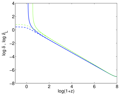
Figure 1: Evolution of the density contrast $\delta$, and linear density contrast $\delta_{L}$ for the 2EXP model with $(\alpha,\beta)=(6.2,0.1)$. Solid line: density contrast in homogeneous case; dashed line: linear density contrast in homogeneous case; thin solid line: density contrast in inhomogeneous case; thin dashed line: linear density contrast in inhomogeneous case.

We can now compute the linearly extrapolated density threshold above which structures will end up collapsing, i.e. $\delta_{c}(z)=\delta_{L}(z=z_{\rm col})$. This quantity, is essential to compute the number of collapsed structures following the Press-Schechter formalism ((1974)). In our analysis we integrate the equations of motion from very high redshifts ($1+z_{i}=10^{8}$) to minimize the effect of the decaying mode on the evolution of the perturbations.

For homogeneous scalar field dark energy, the solution of Eq. (2.2) for a component $\phi$ of fixed contribution to the total energy density $\Omega_{\phi}=1-\Omega_{\rm m}=3/\alpha^{2}$ (as it is the case of dark energy models with an exponential term dominant at early times) and neglecting the radiation component, is:

$$\delta_{c}(z_{\rm col})=\frac{\delta_{i}}{2}\,(1+A^{-1})\left(\frac{1+z_{i}}{1+z_{\rm col}}\right)^{(A-1)/4}\,,$$ (18)

where $A=\sqrt{25-72/\alpha^{2}}$ and we have neglected the decaying mode. Given that $72/\alpha^{2}=24(1-\Omega_{\rm m})$ and that $1+z\propto t^{-2/3}$, we obtain the time dependence $\delta\propto t^{m}$, where $m=(\sqrt{1+24\Omega_{\rm m}}-1)/6$, found by (2003), however, in the context of a scaling tachyon. In an Einstein-de Sitter Universe (i.e. $\alpha=\infty$), solving Eq. (7) with $1+z_{i}=10^{8}$ for an initial perturbation $\delta_{i}=10^{-7}$, the overdensity region collapses at redshift $z_{\rm col}=2.558$, hence $\delta_{c}=1.686$ (see e.g. Padmanabhan (1995)). This classical value was used in the seminal paper of (1974). For a model with one pure exponential potential with $\alpha=6.2$ we would obtain for the same initial conditions $z_{\rm col}=0.522$ and $\delta_{c}=1.681$. This is the asymptotic value of $\delta_{c}$ for the dark energy model considered, $(\alpha,\beta)=(6.2,0.1)$, at high redshifts (see upper panel of figure 2). At low redshifts, when the dark energy component becomes important, the value of $\delta_{c}$ decreases with the redshift of collapse.

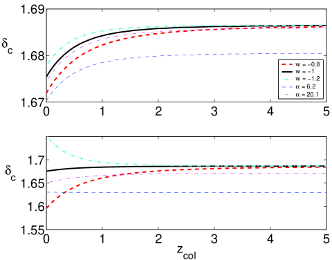
Figure 2: Linear density contrast at the time of collapse in the homogeneous (top panel) and inhomogeneous (bottom panel) dark energy scenarios.

The computation of the value of $\delta_{c}$ at the time of collapse for inhomogeneous dark energy must consider in addition the terms in $\delta_{\phi}$ and $\delta w_{\phi}$ in Eq. (2.2). We can set them to vanish as initial conditions, however, they are going to evolve in cosmological times, in fact, for a pure exponential potential, $\delta_{L}$ and $\delta_{\phi}$ will approach an attractor solution. Indeed, defining the dimensionless quantities:

$$\psi\equiv\frac{\kappa\delta\phi}{\delta_{L}}\,,\hskip 14.22636pt\sigma\equiv\frac{\kappa\delta\phi^{\prime}}{\delta_{L}}\,,\hskip 14.22636pt\tau\equiv\frac{\delta_{L}^{\prime}}{\delta_{L}}\,,$$ (19)

where a prime means differentiation with respect to $\ln a$, we can rewrite Eqs.(2.2) and (16) in the form of a system of first order differential equations

$$\psi^{\prime} = \sigma-\tau\psi\,,$$ (20)

$$\sigma^{\prime} = -\frac{9}{2}\psi-\frac{3}{2}\sigma+\frac{3}{\alpha}\tau-\tau\sigma\,,$$ (21)

$$\tau^{\prime} = \frac{9}{2\alpha}\psi+\frac{6}{\alpha}\sigma-\frac{1}{2}\tau-\tau^{2}+\frac{3}{2}\left(1-\frac{3}{\alpha}\right)\,.$$ (22)

This system has stable critical points at

$$\psi_{c}=\frac{3}{7\alpha}\,,\hskip 14.22636pt\sigma_{c}=\frac{3}{7\alpha}\,,\hskip 14.22636pt\tau_{c}=1\,,$$ (23)

where we have used the well known scaling solution result for an exponential potential $\kappa\phi^{\prime}=1/\alpha$ and $\kappa^{2}V=9H^{2}/2\alpha^{2}$ ( 1998). Substituting back into $\delta_{\phi}$ and $\delta w_{\phi}$ we obtain that $\delta_{\phi}=-\delta_{L}/14$ and $\delta w_{\phi}=5\delta_{L}/14$ independent of $\alpha$. Upon substitution into Eq. (2.2) we find the interesting result

$$\ddot{\delta}_{L}=-2H\dot{\delta}_{L}+\frac{3}{2}H^{2}\delta_{L}\,,$$ (24)

i.e., the linear overdensity evolves in the attractor as if there is only dust in the Universe. However we should not expect to obtain $\delta_{c}=1.686$ as in the Einstein-de Sitter Universe, for two reasons. Firstly, the system takes a finite amount of time before reaching the attractor solution. Secondly, the equation of state evolves inside the collapsing region from $w=0$ at high redshifts to $w=1$ at the time of collapse (see Fig. 3), thus increasing $\rho_{\phi}$ in the cluster favoring the clustering of dark matter. Hence, for the same initial conditions, the collapse occurs earlier, when the growth factor is smaller and therefore $\delta_{c}<1.686$.

One can understand why the equation of state of dark energy evolves inside the overdensity region by inspecting equation (11). Indeed, after the turn around $\dot{r}/r$ becomes negative switching the frictional into an anti-frictional term in the equation of motion of the scalar field. As the scalar potential becomes less and less important the kinetic energy of the field approaches the asymptotic evolution $\dot{\phi}^{2}\propto r^{-6}$ (therefore an effective $w_{\phi_{c}}=1$) which would in principle overtake the energy density of pressureless matter as $\rho_{{\rm m}c}\propto r^{-3}$. In reality, this will never happen, since the singularity in the collapse will not be reached. The dark matter halo will virialise much before and a dynamical equilibrium will be reached, where the halo has a constant radius (the virial radius).

It is important to notice that though the equation of state for dark energy inside the overdensity can become positive, it is still negative in the cosmological background (see figure 3). Hence, the Universe’s background expansion will not be affected by the local behaviour of the dark energy inside clusters. The usual late time accelerated expansion still occurs as normally measured by SNIa. The only effects due to the positivity of the dark energy equation of state occur only inside the overdensities ( 2004). Moreover, within the models investigated, the dark energy contribution inside the cluster is always subdominant when compared to the one of dark matter and it only becomes dominant very near the collapse. We should not expect, therefore, any unusual effects on the virialisation process resulting from the positivity of the equation of state inside the cluster, at least for those models with negligible background dark energy contribution at high redshifts. Signatures in lensing and X-ray observations ( 2004, 2004, 2004) may be noticed though, if dark energy provides a non negligible background contribution at high redshifts.

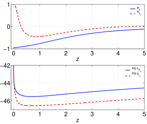
Figure 3: Upper panel: evolution of the dark energy equation of state inside the overdense region (dashed line) and in the background (solid line) for a cluster that collapses today ($z_{\rm col}=0)$. This figure results from numerically integrating the equations of motion of the scalar field with the 2EXP model with $(\alpha,\beta)=(6.2,0.1)$. The turn around occurs at $z_{\rm ta}=0.7$ which is shortly before the redshift at which the equation of state inside the overdensity itself turns its evolution towards unity in opposition to its counterpart in the background that continues to decrease to more negative values. Lower panel: evolution of the dark energy (dashed line) and dark matter (solid line) energy densities in the overdense region. The dark energy contribution only becomes dominant very close to the collapse when $w_{\phi_{c}}$ approaches unity.

In Fig. 2, we show the dependence of $\delta_{c}$ on the redshift of collapse for homogeneous and inhomogeneous dark energy. Note that for the cases of inhomogeneous scalar field dark energy, the value of $\delta_{c}$ at high redshifts is considerably lower than for $w_{\phi}={\rm constant}$ cases. It is worth noting that for an inhomogeneous dark energy, the evolution of $\delta_{c}$ with redshift is significantly altered for the ’phantom energy’, with $\delta_{c}$ decreasing from 1.753 to 1.686 for increasing redshift. These variations of the density threshold will obviously modify the predicted numbers of collapsed objects.

The reason why one finds a difference in $\delta_{c}$ when comparing homogeneous and inhomogeneous dark energy models, becomes clear when one analyses the Poisson equation for the gravitational potential, $\Phi$, inside the overdensity,

$$\nabla^{2}\Phi=\frac{\kappa^{2}}{2}(\rho_{\rm total}+3p_{\rm total})\,.$$ (25)

In the case of homogeneous models

$$\nabla^{2}\Phi = \frac{\kappa^{2}}{2}\left[\rho_{{\rm m}_{c}}+(1+3w_{\phi})\rho_{\phi_{c}}\right]$$ (26)

$$= \frac{\kappa^{2}}{2}\left[(1+\delta)\rho_{{\rm m}}+(1+3w_{\phi})\rho_{\phi}\right]\,,$$

as $\rho_{\phi_{c}}=\rho_{\phi}$. However for inhomogeneous models, making use of equation (17) for a constant equation of state, we have

$$\nabla^{2}\Phi=\frac{\kappa^{2}}{2}\left[(1+\delta)\rho_{{\rm m}}+(1+3w_{\phi})\left(\frac{1+\delta}{1+\delta_{i}}\right)^{1+w_{\phi}}\rho_{\phi}\right]\,.$$ (27)

Comparing equations (26) and (27) one notices that in the inhomogeneous case the contribution of the scalar field energy density becomes increasingly important as the density contrast grows. Since $w_{\phi}$ is generally negative, the source term in equation (25) is smaller than in the homogeneous case. Conversely, if $w_{\phi}$ is more negative than $-1$ the contribution of the scalar field is less and less important and the source term is larger than in the homogeneous case. In conclusion, inhomogeneous dark energy models will contribute to the gravitational potential inside the overdensities in a different way to homogeneous ones. These will clearly affect the whole dynamics of the formation of structures. In particular the late stages of the non-linear collapse of overdensities, such as the time of collapse, virial radius and matter density contrast ( 2004). In the case of dark energy candidates with a dynamical equation of state, such as scalar fields, the effects will be even more interesting. In these cases the source term in equation (25) will vary in time since $w_{\phi_{c}}$ will change during the formation of the collapsing overdensity, resulting in a more complex evolution for the gravitational potential. Recall that $w_{\phi_{c}}$ may even become positive and approach $w_{\phi_{c}}=1$ during the late phase of collapse. Hence the dark energy pressure in equation (25) will source the gravitational potential positively, in opposition to the usual homogeneous models where $w_{\phi}$ is always negative. The effects will be stronger at low redshifts when dark energy dominates the universe density in the background universe.

For a constant equation of state $w$ the following expressions provide an accurate fit to the evolution of the density contrast as shown in Fig. 2:

$$\delta_{c}(z)=\frac{3}{20}(12\pi)^{2/3}\left[1+\alpha x+\beta x^{2}\right]\,,$$ (28)

where $x=\log(\Omega_{m}(z))$ and for homogeneous dark energy we have

$$\alpha = 0.0061w^{2}+0.0327w+0.0403\,,$$ (29)

$$\beta = -0.0163w^{2}-0.0294w-0.0118\,,$$ (30)

whereas for inhomogeneous dark energy it reads

$$\alpha = 0.1198w^{2}+0.6226w+0.5170\,,$$ (31)

$$\beta = 0.2022w^{2}+0.2877w+0.0860\,.$$ (32)

These expressions are valid for $-1.2<w<-0.6$.

3 Coupled quintessence

Let us now look at the case when the scalar field has a coupling with all or part of the dark matter (see for e.g. (2003); (2002, 2002)). In these models, inhomogeneities in the quintessence field may appear due to two main reasons: The first, which is the same as in minimally coupled models, is the change of the local geometry of the region where the overdensity “lives in”, which is just the general relativistic effect of the spacetime deformation. The second is the dragging of the scalar field by the dark matter particles caused by the coupling between them. This second effect is similar to the one which occurs in scalar-tensor theories and leads to inhomogeneities in the scalar field ( 2004; 2004a). Due to these causes, it is then natural to expect stronger inhomogeneity effects in this kind of models than in the minimally coupled one.

The background quantities and the ones who live inside the collapsing region are given by

$$\rho_{\rm um} = \rho_{0}\Omega_{\rm um0}\left(\frac{a_{0}}{a_{i}}\right)^{3}\left(\frac{a_{i}}{a}\right)^{3}\,,$$ (33)

$$\rho_{\rm cDM} = \rho_{0}\Omega_{\rm cDM0}\left(\frac{a_{0}}{a_{i}}\right)^{3}\left(\frac{a_{i}}{a}\right)^{3}e^{B(\phi)-B(\phi_{0})}\,,$$ (34)

$$\rho_{{\rm um}c} = (1+\delta_{i})\rho_{0}\Omega_{{\rm um}c0}\left(\frac{a_{0}}{a_{i}}\right)^{3}\left(\frac{r_{i}}{r}\right)^{3}\,,$$ (35)

$$\rho_{{\rm cDM}c} = (1+\delta_{i})\rho_{0}\Omega_{{\rm cDM}c0}\left(\frac{a_{0}}{a_{i}}\right)^{3}\left(\frac{r_{i}}{r}\right)^{3}e^{B(\phi_{c})-B(\phi_{0})}\,,$$

where the subscripts “um” and “cDM” mean uncoupled matter and coupled dark matter, respectively. Uncoupled matter corresponds to both baryons and to uncoupled dark matter. The function $B(\phi)$ represents the coupling between dark energy and dark matter. In the model discussed by (2000) and (2000), $B(\phi)=-C\kappa\phi$, where $C$ is a constant. But other forms for this function have also been suggested ((2002); Mainini $\&$ Bonometo (2004)).

The total energy densities inside the cluster and the background are therefore, $\rho_{\rm m}=\rho_{\rm um}+\rho_{\rm cDM}$ and $\rho_{c}=\rho_{{\rm um}c}+\rho_{{\rm cDM}c}$ which evolve accordingly to

$$\dot{\rho}_{\rm m} = -3\frac{\dot{a}}{a}\rho_{\rm m}+\frac{dB}{d\phi}\rho_{\rm cDM}\dot{\phi}\,,$$ (37)

$$\dot{\rho}_{c} = -3\frac{\dot{r}}{r}\rho_{c}+\frac{dB}{d\phi_{c}}\rho_{{\rm cDM}c}\dot{\phi_{c}}\,.$$ (38)

If we take for initial conditions $\phi_{c}(a=a_{i})=\phi(a=a_{i})$ we can define $r_{i}=a_{i}/(1+\delta_{i})^{1/3}$ and then we can write $1+\delta\equiv\rho_{c}/\rho_{\rm m}$, as

$$1+\delta=\left(\frac{a}{r}\right)^{3}\frac{\Omega_{{\rm cDM}c0}e^{B(\phi_{c})-B(\phi_{0})}+\Omega_{{\rm um}c0}}{\Omega_{{\rm cDM}0}e^{B(\phi)-B(\phi_{0})}+\Omega_{{\rm um}0}}\,.$$ (39)

It will become useful to write the ratios $G=G(\phi)\equiv\rho_{\rm cDM}/\rho_{\rm m}$ and $G_{c}=G(\phi_{c})\equiv\rho_{{\rm cDM}c}/\rho_{\rm m}(1+\delta)$ in the following form:

$$G(\phi)=\frac{\Omega_{{\rm cDM}0}e^{B(\phi)-B(\phi_{0})}}{\Omega_{{\rm cDM}0}e^{B(\phi)-B(\phi_{0})}+\Omega_{{\rm um}0}}\,.$$ (40)

The time derivative of the density contrast will now have a component coming from the coupling $dB/d\phi$ in the equations above

$$\dot{\delta}=3(1+\delta)\left[\frac{\dot{a}}{a}-\frac{\dot{r}}{r}\right]+(1+\delta)F(\phi)\,,$$ (41)

(compare with equation (9)) where have defined $F(\phi)$ as

$$(1+\delta)F(\phi) = \frac{dB}{d\phi_{c}}\frac{\rho_{{\rm cDM}c}}{\rho_{\rm m}}\dot{\phi}_{c}-\frac{dB}{d\phi}\frac{\rho_{{\rm cDM}}}{\rho_{\rm m}}\dot{\phi}(1+\delta)\,,$$ (42)

$$= (1+\delta)\left[\frac{dB}{d\phi_{c}}G_{c}\dot{\phi}_{c}-\frac{dB}{d\phi}G\dot{\phi}\right]\,,$$ (43)

and it results that $\dot{F}(\phi)$ is

$$\dot{F}(\phi) = G\left[\frac{d^{2}B}{d\phi_{c}^{2}}\dot{\phi}_{c}^{2}+\left(\frac{dB}{d\phi_{c}}\right)^{2}\dot{\phi}_{c}^{2}(1-G_{c})+\frac{dB}{d\phi_{c}}\ddot{\phi}_{c}\right]$$

$$- G\left[\frac{d^{2}B}{d\phi^{2}}\dot{\phi}^{2}+\left(\frac{dB}{d\phi}\right)^{2}\dot{\phi}^{2}(1-G)+\frac{dB}{d\phi}\ddot{\phi}\right]\,.$$

The equations of motion for the evolution of the scalar field inside and the background are in this case:

$$\ddot{\phi} = -3\frac{\dot{a}}{a}\dot{\phi}-\frac{dV}{d\phi}-\frac{dB}{d\phi}\rho_{\rm cDM}\,$$ (45)

$$\ddot{\phi}_{c} = -3\frac{\dot{r}}{r}\dot{\phi}_{c}-\frac{dV}{d\phi_{c}}-\frac{dB}{d\phi_{c}}\rho_{{\rm cDM}c}+\frac{\Gamma_{\phi}}{\dot{\phi}_{c}}\,.$$ (46)

Using these equations we are now able to obtain the modified equation for the non-linear evolution of the density contrast

$$\ddot{\delta} = -2\frac{\dot{a}}{a}\left[\dot{\delta}-(1+\delta)F\right]+\frac{\kappa^{2}}{2}\rho_{\rm m}(1+\delta)\delta+\frac{4}{3}\frac{\dot{\delta}^{2}}{1+\delta}$$ (47)

$$+\frac{\kappa^{2}}{2}\left[(1+3w_{\phi_{c}})\rho_{\phi_{c}}-(1+3w_{\phi})\rho_{\phi}\right](1+\delta)$$

$$-\frac{2}{3}F\dot{\delta}+\frac{1}{3}(1+\delta)F^{2}+(1+\delta)\dot{F}\,.$$

From linearizing the expression of the density contrast one gets

$$\ddot{\delta}_{L} = -2H(\dot{\delta}_{L}-f)+\dot{f}$$ (48)

$$+\frac{\kappa^{2}}{2}\left[\rho_{m}\delta_{L}+(1+3w_{\phi_{c}})\delta_{\phi}~{}\rho_{\phi}+3\rho_{\phi}\delta w_{\phi}\right]\,.$$

where $\delta\phi$ is determined through the equation of motion

$$\delta\ddot{\phi} = -3H\,\delta\dot{\phi}-\frac{dB}{d\phi}\,G\,\rho_{m}\delta_{L}+(\dot{\delta}_{L}-f)\dot{\phi}$$

$$-\left[\frac{d^{2}V}{d\phi^{2}}+\left(\frac{dB}{d\phi}\right)^{2}\,G\,(1-G)\,\rho_{m}+\frac{d^{2}B}{d\phi^{2}}\,G\,\rho_{m}\right]\delta\phi\,,$$

and $f$ is the linearization of $F$:

$$f=G\left[\frac{dB}{d\phi}\,\delta\dot{\phi}+\left(\frac{dB}{d\phi}\right)^{2}(1-G)\dot{\phi}\,\delta\phi+\frac{d^{2}B}{d\phi^{2}}\,\dot{\phi}\,\delta\phi\right]\,.$$ (50)

Assuming a pure exponential potential $V(\phi)=V_{0}\exp(\alpha\kappa\phi)$ with $\alpha=10$, and $B(\phi)=-C\kappa\phi$, we compare in figure 4 the evolution of the linear density contrast at the time of collapse, $\delta_{c}$, between homogeneous and inhomogeneous dark energy. We take into consideration the case when all the dark matter is coupled with the scalar field, or in other words, that the uncoupled matter is only the baryons, hence $\Omega_{\rm um0}=\Omega_{b0}$; and the possibility that only a small fraction of the dark matter feels the field in which case we have taken $\Omega_{\rm um0}=0.25$ in figure 4. Similarly to what happens in minimally coupled models, there are clear differences in the evolution of $\delta_{c}$ between inhomogeneous and homogeneous models. As expected, these differences are more distinct in the case where the amount of coupled dark matter is larger (dashed-lines in figure 4).

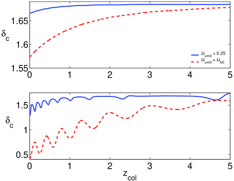
Figure 4: Linear density contrast at the time of collapse in the homogeneous (top panel) and inhomogeneous (bottom panel) coupled quintessence scenarios.

A particular feature is the oscillating behaviour of $\delta_{c}$ that is amplified in the inhomogeneous case. These oscillations are a result of the oscillations performed by the scalar field around the late time attractor solution. As we can see from Eqs. (34) and (3), these oscillations induce a corresponding oscillation in the $\rho_{\rm cDM}$ and $\rho_{{\rm cDM}c}$ components (see Fig. 7 of Copeland et al. (2004)).

Though these oscillations appear inexistent in the homogeneous scenario they are nonetheless present as can be seen by computing $\delta_{c}^{\prime}/\delta_{c}=(d\delta_{c}/dz)/\delta_{c}$, see Fig. 5. They only seem inexistent because the mean $\delta_{c}$ evolves quicker than the amplitude of the oscillations. For the inhomogeneous case, however, the scalar field enters a regime of amplified oscillations inside the overdensity after the turn around (as the $\dot{\phi}_{c}$ term in Eq. (46) becomes anti-frictional), hence its oscillations are progressively larger. Consequently, the oscillations in $\delta_{c}$ are more probable of becoming visible.

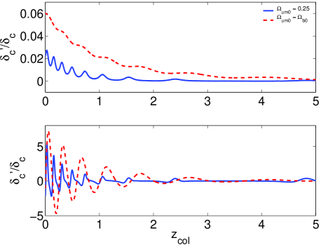
Figure 5: Ratio $\delta_{c}^{\prime}/\delta_{c}$ where prime is differentiation with respect to redshift for homogeneous (top panel) and inhomogeneous (bottom panel) coupled quintessence scenarios.

4 Summary and Conclusions

During the highly non-linear regime of cosmological perturbations, when dark matter halos are formed, scalar fields may become inhomogeneous. Hence, evolving differently inside a collapsed overdensity and in the background Universe. The reason is simple: Different local spacetime geometries lead to different local equations of motion for the field. In the case of dark energy candidates, such as quintessence, this may result on dark energy having a different equation of motion in the background Universe and inside clusters. As a consequence, the dynamics of non-linear structure formation in the universe may show a distinct signature associated to the nature of dark energy and a particular model ( 2004).

The behaviour of dark energy during the non-linear regime of structure formation can be divided into two major groups: the inhomogeneous models, which are the ones where the field inside the overdensity behaves differently form the background Universe and the homogeneous ones, where dark energy is just a smooth fluid which bath the whole Universe.

In this article we have investigated the effects of inhomogeneities in dark energy on the time of collapse of a dark matter overdensity, and how this is reflected on the linearly extrapolated density threshold above which structures will end up collapsing, i.e. $\delta_{c}(z)=\delta_{L}(z=z_{\rm col})$. We have studied both coupled and minimally coupled scalar field candidates to dark energy as well as fluids with a constant equation of state. We have compared all these models and we found distinct features among them when taking into account the possible inhomogeneities in the dark energy fluid during the non-linear regime.

In general $\delta_{c}(z)$ depends on the particular model one considers. For constant equation of state candidates to dark energy there are minor differences between homogeneous and inhomogeneous models. The exception to that are the phantom energy candidates, with $w_{\phi}<-1$. These present a quite distinct behaviour when one takes into account the inhomogeneities in the dark energy fluid. However, it is on scalar fields candidates where inhomogeneities in the dark energy fluid may result in more concrete features. The later will depend on its dynamical equation of state, which can be scale dependent, and on the contribution of the field to the energy budget of the Universe both at low and high redshifts. Coupled quintessence models behave similarly to the minimally coupled field candidates, but naturally show a strong dependence on the amount of dark matter coupled to the scalar field and the strength of the coupling.

The reason for such a difference between inhomogeneous and homogeneous models can be understood looking at the Poisson equation (25) which gives the evolution of the gravitational potential inside the clusters. In opposition to the homogeneous models, one cannot neglect the importance of dark energy inside the matter overdensities. This leads to an extra source term in the usual Poisson equation, which affects the overall behaviour of the gravitational potential. This effect is specially important when the collapsing region enters into the non-linear regime. In particular, the time of collapse of the overdensity depends on the dark energy model one considers and on the equation of state inside it. These effects are reflected into linearly extrapolated density threshold above which structures will end up collapsing, $\delta_{c}$.

The results of this work may have important consequences on cosmological studies of structure formation. In particular one can study its implications for the number density of dark matter halos, their density profiles, galaxy number counting and dark matter halo concentrations ( 2005, 2004). These investigations are imperative for cosmological studies that rely on these ingredients to measure dark energy. Examples of these studies, for the case of homogeneous dark energy models, include semi-analytical studies of strong lensing statistics ( 2003, 2004) and weak lensing number counts ( 2003). And for inhomogeneous models include a study of dark matter halo concentrations ( 2004).

Many other astrophysical phenomena may reflect the inhomogeneities in dark energy fluid during the non-linear regime. For instance, the merger of dark matter halos depend on the gravitational potential between them. Effects on the evolution and magnitude of the gravitational potential, may also affect peculiar velocities of galaxies inside clusters. One should also point out here, that in low-density regions of the universe, such as voids, inhomogeneous dark energy models, may play an important role as well. In those regions the local spacetime geometry may be different from the usual Friedman-Robertson-Walker metric one usually assumes for the background Universe. It is natural to think that dark energy inside voids may behave differently from its background behaviour. This may again affect the dynamics of formation of voids in the universe. All these effects could in principle be detected using galaxy redshift surveys such as the Sloan Digital Sky Survey ( 2003, 2002).

ACKNOWLEDGMENTS
DFM is supported by Fundacão Ciência e a Tecnologia. NJN is supported by the Particle Physics and Astronomy Research Council (PPARC) and is thankful to Nabila Aghanim and António da Silva for useful discussions and hospitality at IAS Orsay, during the initial stages of this work. The authors also thank Ana Lopes for comments on the manuscript.

References

- (1) Abazajian K., et al. [SDSS Collaboration], 2003, Astron. J. 126, 2081
- (2) Alcubierre A., Guzman F., Matos T., Nunez D., Urena-Lopez L., Wiederhold P., 2002, Class. Quant. Grav., 19, 5017.
- (3) Amendola L., 2000, Phys. Rev. D 62 043511.
- (4) Amendola L., and Tocchini-Valentini D., 2001, Phys. Rev. D 64 043509.
- (5) Amendola L., 2003, preprint astro-ph/0311175.
- (6) Amendola L., and Tocchini-Valentini D., 2002, Phys. Rev. D 66 043528.
- (7) Arbey A., Lesgourgues J., Salati P., 2001, Phys. Rev. D, 64, 123528.
- (8) Bagla J., Jassal H., Padmanabhan T., 2003, Phys. Rev. D, 67, 063504.
- (9) Barreiro T., Copeland E. Nunes N.J., 2000, Phys. Rev. D, 61, 127301
- (10) Bartelmann M., Meneghetti M., Perrotta F., Baccigalupi C., Moscardini L., 2003, AA, 409, 449.
- (11) Bean R. Magueijo J., 2002, Phys. Rev. D, 66, 063505.
- (12) Brax P. Martin J. 1999, Phys. Lett. B, 468, 40.
- (13) Caldwell R., 2002, Phys. Lett. B 545 23.
- (14) Carroll S.M., Press W.H. Turner E.L., 1992, Ann. Rev. Astron. Astrophys., 30, 499.
- (15) Causse M., 2003, preprint astro-ph/0312206.
- Colless et al. (1998) Colless M., 1998, ”First results from the 2dF galaxy redshift survey”, astro-ph/9804079
- (17) Clifton T., Mota D.F., Barrow J.D., 2004, preprint gr-qc/0406001.
- (18) Copeland E.J., Liddle A.R., Wands D., 1998, Phys. Rev. D 57 4686.
- Copeland et al. (2004) Copeland E.J., Nunes N. J., and Pospelov M., 2004, Phys. Rev. D 69, 023501.
- (20) Ferreira P, and Joyce M., 1998, Phys. Rev. D 58 023503.
- (21) Guzman F., Urena-Lopez L. 2003, Phys. Rev. D, 68, 024023.
- (22) Holden D.J., and Wands D., Phys. Rev. D 61 043506.
- (23) Hwang J. c., Noh H., Phys. Rev. D 64 103509.
- (24) Jassal H., Bagla J. S., Padmanabhan T., 2005, Phys.Rev.D72:103503.
- (25) Khoury J., Weltman A., 2004, Phys. Rev. D 69 044026.
- (26) Khoury J., Weltman A., 2003, preprint astro-ph/0309300.
- (27) Knop R.A., et al., ApJ, 2003, 598, 102.
- (28) Lopes A.M. Miller L., 2004, MNRAS, 348, 519.
- (29) Lopes A.M., Mota D. F. Miller L., 2004, submitted to AA.
- Maor Lahav (2004) Maor I., Lahav O., 2004, JCAP 0507:003.
- Mainini Bonometo (2004) Mainini R., Bonometo S.A., preprint astro-ph/0406114.
- (32) Manera M. Mota D.F. astro-ph/0504519.
- (33) Mota D.F., Barrow J.D., 2004a, Phys. Lett. B, 581, 141.
- (34) Mota D.F., Barrow J.D., 2004b, MNRAS, 349, 281.
- (35) Mota D.F. van de Bruck C., 2004, AA, 421, 71.
- (36) Nunes N. J., da Silva A. C. Aghanim N., 2005, AA in print, e-Print Archive: astro-ph/0506043.
- Padmanabhan (1995) Padmanabhan, T. 1995, Structure formation in the universe, Cambridge University Press
- (38) Padmanabhan T., 2002, Phys. Rev. D 66, 021301.
- (39) Padmanabhan T., Choudhury T., 2002, Phys. Rev. D, 66, 081301.
- (40) Wang P., 2005, astro-ph/0507195.
- (41) Percival W., 2005,astro-ph/0508156.
- (42) Perlmutter S., et al., 1999, ApJ, 517, 565.
- (43) Press W., Schechter P., 1974, Astrophys. J. 187 425.
- (44) Ratra B., Peebles P.,1988, ApJ, 325, L17.
- (45) Riess A.G., et al., 2001, ApJ., 560, 49.
- (46) Riess A.G. et al. [Supernova Search Team Collaboration],2004, Astrophys. J. 607, 665.
- (47) Sereno M. Longo G., 2004, MNRAS, 354, 1255.
- (48) Spergel D.N., et al., 2003, ApJ Suppl., 148. 175.
- Tegmark et al. (2004) Tegmark et al., 2004, Phys. Rev. D69, 103501.
- (50) Tocchini-Valentini D., and Amendola L., 2002, Phys. Rev. D 65 063508
- (51) Wang L.M. Steinhardt P.J., 1998, ApJ, 508, 483.
- (52) Wetterich C., 2001, Phys. Lett. B, 522, 5.
- (53) Wetterich C., 2002, Phys. Rev. D, 65, 123512.
- (54) Zehavi I., et al. [SDSS Collaboration], 2002, Astrophys. J. 571, 172.
- (55) Zlatev I., Wang L., and Steinhardt P., 1999, Phys. Rev. Lett. 82, 896.