What are the environments of lens galaxies?

Abstract

Using measured tangential shear profiles and number counts of massive elliptical galaxies, the halo occupation distribution of strong lensing galaxies is constrained. The resulting HOD is then used to populate an N-body simulation with lens galaxies, in order to assess the importance of environment for strong lensing systems. Typical estimated values for the convergence and shear produced by nearby correlated matter are ${\kappa_{\rm grp}}\simeq{\gamma_{\rm grp}}\simeq 0.03$, with much stronger events occurring relatively infrequently. This implies that estimates of quantities like the Hubble constant are not expected to be significantly biased by environmental effects. One puzzle is that predicted values for the external shear at lens galaxies are far below the values obtained by modeling of strong lensing data.

1. Introduction

Strong gravitational lensing has emerged as an important tool in the astrophysical toolbelt. Strong lenses have been used, for example, to measure the Hubble constant (e.g Schechter, 2004, and references therein), to study the properties of elliptical galaxies (e.g. Rusin et al., 2003), to study dark matter substructure (e.g. Kochanek & Dalal, 2004), to resolve the inner structure of quasars (Richards et al., 2004), even to constrain the geometry of the universe (Broadhurst et al., 2004). Many of the applications of strong lensing require reconstructing the gravitational potential of the lens, which includes contributions both from the principal lens galaxy and from any (projected) nearby structures. Models of strong lenses often treat the lens galaxy itself in exquisite detail (e.g Cohn et al., 2001), however the lens environment is usually treated more simply. Except in cases with obvious nearby galaxies (e.g. Koopmans et al., 2003; Kundic et al., 1997), the environments of lenses are typically modeled simply as tidal shear.

How valid is this approximation? In some instances, higher order terms in the potential than the $\sim r^{2}\cos 2\theta$ term represented by external shear may be required, and Kochanek (2004) describes quantitatively how to estimate the importance of such terms for a lens model. Additionally, the nearby environment can contribute not only tidal shear, but (projected) mass density as well. As discussed by Holder & Schechter (2003), massive ellipticals are biased tracers of the underlying mass density; we expect massive ellipticals to reside in overdense environments, and indeed, many lens galaxies are found in poor groups or galaxy clusters. Keeton & Zabludoff (2004), among others, point out that the environmental mass density, here denoted ${\kappa_{\rm grp}}$, can lead to a mass sheet degeneracy in many of the quantities derived from strong lensing analyses. For instance, the Hubble constant inferred from time delays scales as $H_{0}\propto(1-{\kappa_{\rm grp}})$. In the age of precision cosmology, it is clearly important to determine the magnitude of this uncertainty in lens models.

In principle, our theory of structure formation should already provide an answer to this question. In the cold dark matter (CDM) model, the clustering of mass proceeds largely through the growth and merging of dark matter halos. Assessing the importance of lens environments reduces basically to determining, where (in which halos) do lens galaxies live? Placing lens galaxies chiefly in the most massive, biased objects like galaxy clusters will of course enhance the effects of environment, whereas environment will be less important if lenses live in lower mass halos.

We do not have complete freedom to pick the halo occupation distribution of lens galaxies, however: there are now several observational constraints on models for elliptical galaxies and their hosts. First, galaxy-galaxy lensing (Sheldon et al., 2004; Seljak et al., 2004) provides direct constraints on the average mass profiles surrounding lens galaxies. Second, choosing a model for the halo occupation distribution of galaxies implicitly makes a prediction for the number density of those galaxies, and there are now precise measurements of the number density of massive elliptical galaxies (which most strong lenses are). Accordingly, we can use these measurements to constrain the HOD of lens galaxies, and thereby compute the effects of lens environments.

The plan of this paper is as follows. In §2, the number counts of Sheth et al. (2003) and the galaxy-galaxy lensing results of Sheldon et al. (2004) are combined, in the context of the halo model, to constrain the halo occupation distribution of lens galaxies. In §3, this HOD is used to populate an N-body simulation with lens galaxies, which is then exploited to make predictions for the effects of lens environments.

2. Halo model calculation

Hu & Jain (2003) explain in detail how the halo model may be used to compute the number density and average surface density (and shear) profiles around galaxies. As they discuss, the galaxy-convergence angular correlation function may be computed by projecting the 3-D galaxy-mass power spectrum using the Limber (1954) approximation,

$$\langle\kappa\rangle(\theta) = \int\frac{ldl}{2\pi}J_{0}(l\theta)C_{l}^{g\kappa},$$ (1)

$$C_{l}^{g\kappa} = \int_{0}^{z_{\rm src}}dzW_{g}(z)W_{\kappa}(z)\frac{P_{g\delta}(k=l/r(z))}{r^{2}(z)c/H(z)},$$ (2)

$$W_{g}(z) = {\bar{n}}_{A}^{-1}\;r^{2}(z)\frac{c}{H(z)}{\bar{n}}_{V}(z),$$ (3)

$$W_{\kappa}(z) = \frac{3}{2}\Omega_{m}H_{0}^{\;2}\frac{(1+z)r(z)}{c\,H(z)}\frac{D_{LS}}{D_{S}}.$$ (4)

Here, ${\bar{n}}_{V}(z)$ is the volume number density of lens galaxies as a function of redshift, ${\bar{n}}_{A}=\int dzr^{2}(z)\frac{c}{H(z)}{\bar{n}}_{V}(z)$ is the projected angular number density of lens galaxies, $r(z)$ is the comoving angular diameter distance, and $D_{LS,S}$ are the angular diameter distances from lens to source and from observer to source, respectively.

The halo model enters by providing a prescription for the galaxy-mass power spectrum $P_{g\delta}$. The ingredients are models for the dark matter halo mass function $dn_{h}/dM$, the halo bias $b(M)$, the halo density profile $\rho(r)$, and the halo occupation distribution of galaxies. For DM halos, we use the mass function and bias prescription of Sheth & Tormen (1999), the density profile of Navarro et al. (1997), and halo concentrations of Bullock et al. (2001). The halo occupation distribution (HOD) specifies how galaxies populate DM halos. Kravtsov et al. (2004) present a model for the HOD based upon N-body simulations. In their model, the mean number of galaxies (say, brighter than luminosity $L$) residing in halos of mass $M$ has two pieces, ${\bar{N}}(M)={\bar{N}}_{c}(M)+{\bar{N}}_{s}(M)$, corresponding to central galaxies and satellite galaxies. They find that $N_{c}(M)$ is well fit by a step function, $N_{c}(M)=\Theta(M-M_{\rm th})$ where the parameter $M_{\rm th}$ is the minimum mass halo capable of hosting a central galaxy with the required properties (e.g. luminosity). Kravtsov et al. also find that the satellite term is well described by a Poisson distribution with mean

$${\bar{N}}_{s}(M)=\left(\frac{M}{A_{s}M_{\rm th}}\right)^{m_{s}}$$ (5)

for $M>M_{\rm th}$ and zero otherwise. The halo mass function and HOD together specify the predicted galaxy volume number density, viz

$${\bar{n}}_{V}(z)=\int dm\frac{dn_{h}}{dM}\,{\bar{N}}(M).$$ (6)

Similarly, the halo model expression for the galaxy-mass power spectrum becomes, in the notation of Hu & Jain (2003),

$$P_{g\delta}(k)=I_{1g}(k)I_{1m}(k)P_{\rm lin}(k)+I_{2c}(k),$$ (7)

where

$$I_{1m}(k) = \int dM\frac{M}{\rho_{M}}\,\frac{dn_{h}}{dM}\,b(M)y_{h}$$ (8)

$$I_{1g}(k) = {\bar{n}}_{V}^{\,-1}\int dM[{\bar{N}}_{c}+{\bar{N}}_{s}y_{g}]\frac{dn_{h}}{dM}b(M)$$ (9)

$$I_{2c}(k) = {\bar{n}}_{V}^{\,-1}\int dM\frac{M}{\rho_{M}}\,\left[\frac{dn_{h}}{dM}\,({\bar{N}}_{c}y_{h}+{\bar{N}}_{s}y_{h}y_{g})\right.$$ (10)

$$\left.\qquad+\frac{dn_{s}}{dM}\Theta(M-M_{\rm th})y_{s}\right],$$

$y_{h}$ is the normalized Fourier transform of the DM density profile,

$$y_{h}(k,M)=M^{-1}\int_{0}^{r_{\rm vir}}dr\;4\pi r^{2}\rho(r)\frac{\sin(k\,r)}{k\,r},$$ (11)

and similarly $y_{g}$ is the normalized Fourier transform of the satellite galaxy distribution within halos, here assumed to track the mass, so that $y_{g}=y_{h}$. Note that the redshift-dependent concentration is implicitly included in the density profile $\rho(r,M)$. The satellite mass function is given by

$$\frac{dn_{s}}{dM}=\int_{M}^{\infty}dM_{h}\,m_{s}\left(\frac{M_{h}}{A_{s}M}\right)^{m_{s}}\frac{dn_{h}}{dM_{h}}.$$ (12)

The observables to match are the number density and tangential shear profile. Eqn. 6 gives the predicted number density, while the predicted shear profile is given by

$$\langle\gamma_{T}\rangle(\theta)=\int\frac{l\,dl}{2\pi}C_{l}^{g\kappa}J_{2}(l\theta).$$ (13)

Strong gravitational lenses tend to be massive elliptical galaxies, and Sheldon et al. (2004) report the average shear profile of elliptical galaxies with velocity dispersion $\sigma>182$ km/s observed in the Sloan Digital Sky Survey (SDSS). Sheth et al. (2003) have measured the velocity dispersion function of SDSS ellipticals, and found it to be well fit by a Schechter-type function. For ellipticals with $\sigma>182$ km/s, their fit gives a total number density of $n_{\rm obs}=0.00172({\rm Mpc}/h)^{-3}$. Also, the mean squared velocity dispersion for this sample is $\langle\sigma^{2}\rangle=(216\rm{km/s})^{2}$. For a lens at $z=0.45$ and source at $z_{\rm src}=2$, this would correspond to an Einstein radius of $\theta_{\rm E}=4\pi(\sigma/c)^{2}D_{LS}/D_{S}=0.9\arcsec$, in good agreement with typical lens splittings.

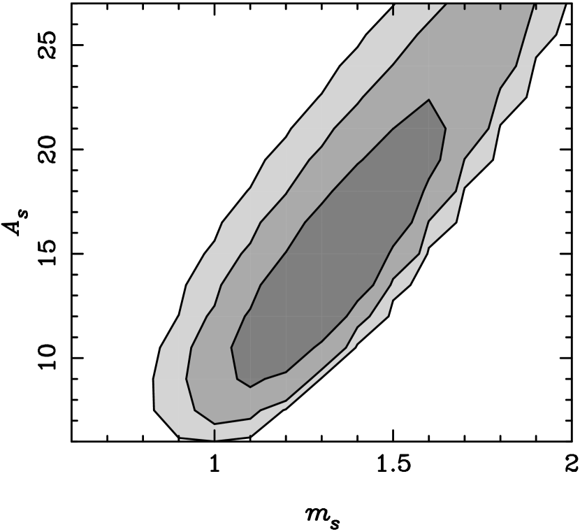
Figure 1.— Plotted are 68, 95, and 99% likelihood contours in the $m_{s}-A_{s}$ plane for $M_{\rm th}=10^{12.5}h^{-1}M_{\odot}$.

The ingredients are now in place to find the HOD parameters which best fit the observed data on massive ellipticals. This HOD will be used in the next section to populate halos found in an N-body simulation, so it is important that consistent definitions of halo mass are used for the halo model calculation and the group finder, the friends-of-friends algorithm with linking length $b=0.2$. Jenkins et al. (2001) have found that FOF with $b=0.2$ corresponds well to halo overdensity of 180, and that the Sheth-Tormen mass function provides a good fit to the mass function if the halo mass is defined not as the virial mass, but as $M=M_{180}$, i.e. the mass enclosed within radius $r_{180}$ for which the average interior density is 180 times the mean matter density $\rho_{M}$. The Bullock et al. (2001) model for halo concentrations is given in terms of the virial mass, not $M_{180}$ which is typically $\sim 1.2\times$ larger than $M_{\rm vir}$. Given the NFW density profile, it would not be difficult to translate from $M_{180}$ to $M_{\rm vir}$ (Hu & Kravtsov, 2003), but the dependence of concentration on mass is so weak ($c_{v}\propto M^{-0.13}$) that this distinction is ignored here.

The HOD used here has three parameters: $M_{\rm th}$, $A_{s}$ and $m_{s}$. Figure 1 shows likelihood contours in the $A_{s}-m_{s}$ plane, for $M_{\rm th}=10^{12.5}h^{-1}M_{\odot}$, assuming a 10% uncertainty for the number density $n_{\rm obs}$. Other values of $M_{\rm th}$ gave significantly poorer fits, so $M_{\rm th}=10^{12.5}h^{-1}M_{\odot}$ will be assumed throughout. As can be seen from the figure, a broad region in the $A_{s}-m_{s}$ plane, centered on $A_{s}=15$, $m_{s}=1.4$ provides reasonable fits to the data. These values compare reasonably well to HOD parameters derived by Zheng et al. (2004) from hydrodynamic simulations and semi-analytic models. The satellite fraction for these HOD parameters is roughly 25%, in good agreement with the estimates of Keeton et al. (2000). There appears to be a mild degeneracy between $A_{s}$ and $m_{s}$, in the sense that increasing $A_{s}$ (which lowers the fraction of lens galaxies that are satellites) may be compensated by increasing $m_{s}$ (which places satellites in more massive groups) to hold fixed the tangential shear profile; see fig. 2 for an example. However note that large $m_{s}$ is likely disfavored by measurements of the multiplicity function in clusters (Kochanek et al., 2003).

One defect which has been glossed over so far is that the SDSS data on elliptical galaxies used to constrain the HOD parameters extend to redshifts $z\lesssim 0.15$, much less than typical lens redshifts $z_{l}\sim 0.5$. In order to apply this HOD to the lens population, it must be assumed that there is little evolution in massive ellipticals between $z=0.15$ and $z=0.5$.

Note that the average ${\kappa_{\rm grp}}$ may be calculated using these HOD parameters using just the halo model, by keeping only the term in $P_{g\delta}$ corresponding to the correlation between satellite galaxies and mass in their parent halos:

$$P_{g\delta}^{\rm grp}(k)=\frac{1}{{\bar{n}}_{V}}\int dM\frac{M}{\rho_{M}}\frac{dn_{h}}{dM}\,{\bar{N}}_{s}\,y_{h}\,y_{g}.$$ (14)

This somewhat underestimates ${\kappa_{\rm grp}}$, because in this formalism halo profiles extend only out to $r_{180}$, whereas in reality there is mass overdensity extending well beyond this radius (e.g. Guzik & Seljak, 2002). With this caveat in mind, applying eqn. 14 gives an average ${\kappa_{\rm grp}}\approx 0.02$. As noted above, fractional errors in (e.g.) the Hubble constant will be ${\cal O}({\kappa_{\rm grp}})$, implying that estimates of the Hubble constant which ignore the group convergence make $\sim 2\%$ errors for most lens systems, which is still small compared to other systematics.

Figure 2.— The galaxy-shear correlation function for massive ellipticals. Data points are from Sheldon et al. (2004), kindly provided in electronic form by D. Johnston (2004, priv. comm.) The solid curves correspond to the predicted $\Delta\Sigma=\Sigma_{\rm crit}\langle\gamma_{T}\rangle$ for three different halo occupation distributions, with $A_{s}=15$, $m_{s}=1.4$; $A_{s}=21$, $m_{s}=1.6$; and $A_{s}=10.5$, $m_{s}=1.2$. The other curves show the contributions to eqns. (7) and (10): the galaxies’ own halos or subhalos (dotted), group halos (dashed), and two-halo term (dash-dot).

3. Application to N-body simulations

The halo occupation distribution from the previous section can now be used to populate halos from an N-body simulation with lens galaxies, to compute the distribution of lens environments. A small (by modern standards) dissipationless simulation with $256^{3}$ particles in a 256 $h^{-1}$Mpc box was run using the TPM code (Bode & Ostriker, 2003) for a WMAP cosmology with $\Omega_{M}=0.27$, $\Omega_{\Lambda}=0.73$ and $h=0.72$. Initial conditions were generated using the GRAFIC1 code (Bertschinger, 2001), for a scale-invariant primordial power spectrum ($n=1$) and present-day amplitude $\sigma_{8}=0.9$. The particle mass for this simulation was $m_{p}=7.49\times 10^{10}h^{-1}M_{\odot}$, so that halos of mass $M=10^{12.5}h^{-1}M_{\odot}$ contained 42 particles. Since the simulation was dissipationless, $\Omega_{B}=0$ was assumed for generating the initial conditions.

The $z=0.45$ output from this simulation was then populated with lens galaxies using the best fitting HOD from the previous section, with $M_{\rm th}=10^{12.5}h^{-1}M_{\odot}$, $A_{s}=13.5$, and $m_{s}=1.3$. First, the friends-of-friends algorithm with linking length $b=0.2$ was used to find halos in the simulation. Central galaxies were placed at the most bound particles in these halos. The number of satellites for each halo was determined by generating random numbers from a Poisson distribution with mean given by eqn. 5. Satellite galaxies were assigned the positions of randomly selected particles in each halo, to match the assumption above that the satellite distribution follows the DM distribution.

Next, convergence and shear (assuming a source redshift $z_{\rm src}=2$) were computed at the galaxy positions by projecting the particle data along three orthogonal axes. For central galaxies, the contribution from the galaxies’ own halos must be removed in order to compute solely environmental effects. This was accomplished by excluding, for each galaxy, all particles in its halo (as defined by FOF) when computing the projected convergence. Applying this method for shear would be computationally onerous, since the shear is computed by repeated Fourier transforms of the full convergence map. Instead, to compute the environmental shear at each central galaxy, comoving 100 $h^{-1}$kpc cavities were excised around each galaxy. This truncated particle list was then projected to make a convergence map with comoving 31.25 $h^{-1}$ kpc resolution, which was then Fourier transformed to produce shear maps of the same resolution. The resulting shear values at the galaxy positions were mildly dependent upon the precise cavity radius; using comoving 50 $h^{-1}$kpc cavities instead of 100 $h^{-1}$kpc cavities gave shear values $\sim 20\%$ larger. For satellite galaxies, no such excision of particles was required, because the satellites were placed randomly inside their parent groups, not on subhalos. The resulting histogram of ${\kappa_{\rm grp}}$ and ${\gamma_{\rm grp}}$ values is plotted in figure 3.

    

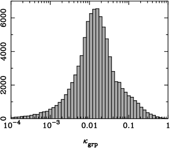
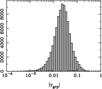
Figure 3.— Histograms of (left) ${\kappa_{\rm grp}}$ and (right) $|{\gamma_{\rm grp}}|$ for the $z=0.45$ simulation, assuming $z_{\rm src}=2$. The HOD used here had $M_{\rm th}=10^{12.5}h^{-1}M_{\odot}$, $A_{s}=13.5$, and $m_{s}=1.3$.

There are a few points to note. First, the mean values of convergence and shear are similar, with $\langle{\kappa_{\rm grp}}\rangle\approx\langle|{\gamma_{\rm grp}}|\rangle\approx 0.03$. This agrees roughly with the simple halo model estimate for $\langle{\kappa_{\rm grp}}\rangle$ given in the previous section. While the ${\gamma_{\rm grp}}$ histogram appears well described by a lognormal distribution, the ${\kappa_{\rm grp}}$ histogram exhibits extended tails.

An interesting related question is that of the frequency of high ${\kappa_{\rm grp}}$ or ${\gamma_{\rm grp}}$. In these simulations, ${\kappa_{\rm grp}}>0.1$ occurred with roughly $\sim 6\%$ probability, while $|{\gamma_{\rm grp}}|>0.1$ had $\sim 3\%$ probability. One difficulty in making these estimates is that the tails of the ${\kappa_{\rm grp}}$ and ${\gamma_{\rm grp}}$ distributions are likely overrepresented, due to projections. Galaxies which project near unrelated massive groups will appear to have higher ${\kappa_{\rm grp}}$ and ${\gamma_{\rm grp}}$ than is truly representative for their own environments. Similarly, galaxies which project near voids will have overly low ${\kappa_{\rm grp}}$. Of course, from the viewpoint of estimating errors on derived quantities like the Hubble constant, such projections are just as important to consider as the immediate environment of the lenses.

One last point to consider is that selection effects can modify the probability distributions for ${\kappa_{\rm grp}}$ and ${\gamma_{\rm grp}}$ for actual lenses compared to the distributions computed here. For example, the strong lensing cross section scales as $(1-{\kappa_{\rm grp}})^{-2}$, so in principle the histograms of convergence and shear should be weighted by this factor (Holder & Schechter, 2003). Reweighting the distributions (excluding the tiny fraction of galaxies with ${\kappa_{\rm grp}}>0.5$), the average $\langle{\kappa_{\rm grp}}\rangle$ increases to 0.037, while $\langle{\gamma_{\rm grp}}\rangle$ increases to 0.033. Another possible selection effect is that ellipticals with higher velocity dispersion (and hence larger lensing cross section $\propto\theta_{\rm E}^{2}\propto\sigma^{4}$) will tend to live in more massive, more biased halos, and so the $\kappa$ and $\gamma$ histograms should be weighted by this factor as well for lenses. Unfortunately, this requires a more detailed halo occupation distribution than has been used here.

4. Discussion

This paper has presented a calculation of the effects of the environments surrounding lens galaxies. Lens galaxies were placed in an N-body simulation using a halo occupation distribution calibrated to match both the number density and tangential shear profiles observed for massive elliptical galaxies in the Sloan Digital Sky Survey. The SDSS results are measured for galaxies at low redshift, $z\lesssim 0.2$, while lens galaxies are typically at higher redshift, $z\approx 0.5$, so the results presented here will be meaningful only if there is little evolution in elliptical galaxies between $z\approx 0.15$ and $z\approx 0.45$. The expected average values for convergence and shear are $\langle{\kappa_{\rm grp}}\rangle\approx\langle|{\gamma_{\rm grp}}|\rangle\approx 0.03$, with a spread of $\sim 0.6$ and $\sim 0.35$ in $\log_{10}$ for $\kappa$ and $\gamma$ respectively. Values much higher than the mean appear relatively rarely, with ${\kappa_{\rm grp}}>0.1$ occurring with $\sim 6\%$ probability and ${\gamma_{\rm grp}}>0.1$ occurring with $\sim 3\%$ probability.

Previous work has considered related topics. Both Keeton et al. (1997) and Holder & Schechter (2003, HS) have estimated the magnitude of tidal shear produced by material correlated with lens galaxies. This paper has followed an approach quite similar to that developed by HS. The results presented here appear similar to those of Keeton et al., however HS find somewhat higher environmental shear. This appears to be due to a different HOD; HS use massive elliptical galaxies produced using the semi-analytic recipes of Kauffmann et al. (1999). As they note, their lens galaxies tend to live in very massive halos, with roughly $\sim 30\%$ residing in clusters more massive than $10^{14}h^{-1}M_{\odot}$. Accordingly, the number density of massive elliptical galaxies predicted by HS is lower than the values computed here by roughly an order of magnitude. Further observations of the environments surrounding lens galaxies (e.g. Fassnacht et al., 2004) can help determine whether lenses typically do reside in such massive halos.

Recently, Keeton & Zabludoff (2004) have investigated the importance of the group convergence on strong lenses. They construct a mock group including several supercritical galaxies separated by a few Einstein radii. By explicit construction, they showed that in cases like these, ${\kappa_{\rm grp}}$ can approach $\sim 0.15-0.2$, which would dramatically skew the results of analyses ignoring group convergence. Clearly, for systems like these, it is necessary to model such close neighbors using both convergence and shear, and indeed in systems like PG 1115+080 the nearby groups are modeled with isothermal spheres or NFW profiles (e.g. Treu & Koopmans, 2002; Kochanek & Dalal, 2004). For the majority of systems, however, the environment is treated merely with tidal shear, and the results of this paper indicate that such a treatment is usually adequate. If typical ${\kappa_{\rm grp}}$ at lens galaxies is $\sim 3\%$, then errors in the Hubble constant will similarly be at the $\sim 3\%$ level, which is still unimportant compared to the $\gtrsim 10\%$ systematic errors typical of lensing $H_{0}$’s.

One remaining puzzle from this work is the origin of the large shears measured at lens galaxies. As discussed by Keeton et al. (1997), successful models of strong lenses typically require external shear at the level of $\gamma\sim 10-15\%$, considerably higher than the ${\gamma_{\rm grp}}\approx 3\%$ found here. Such shear cannot be explained by uncorrelated structure (e.g. line-of-sight projections), which should produce shear of order the cosmic shear, $\sim 1-2\%$ on these scales. HS have argued that such strong shear naturally occurs for lenses living in massive systems like galaxy clusters where $\kappa_{s}=\rho_{s}r_{s}/\Sigma_{\rm crit}\approx 0.15$. On the other hand, Keeton et al. have suggested that much of this so-called external shear originates in the halos of the lens galaxies themselves. To support this idea, they note that the total quadrupole at the images aligns quite well with the galaxy orientation, while misalignments larger than observed would arise if $10-15\%$ external shear were completely uncorrelated with the galaxy orientation (see Kochanek, 2004, for an updated version of this). As noted by Holder (2003, priv. comm.), however, this argument has difficulty. Halo material stratified on ellipses with the same ellipticity as the mass interior to the Einstein ring will produce no effect on the lens images, as shown by Newton. For the halo to produce this shear, it must either have principal axes substantially twisted relative to the galaxy principal axes, or it must have a very different ellipticity. To illustrate, imagine taking an isothermal ellipsoid with Einstein radius $r_{\rm E}$, and beyond some radius $r_{0}$, either twisting the ellipsoidal axes by some angle $\Delta\theta$ or changing the ellipticity by $\Delta\epsilon$. Then the change in shear at the Einstein radius, in the limit $r_{0}\gg r_{\rm E}$, will be of order

$$\Delta\gamma\sim\frac{1}{2\pi}\frac{r_{\rm E}}{r_{0}}\left(\Delta\epsilon+2\epsilon\sin^{2}\Delta\theta\right),$$ (15)

where typical lens Einstein radii are $\simeq 2r_{\rm eff}$ and typical ellipticities are $\epsilon\sim 0.3$. Hoekstra et al. (2004) have found that galaxies and their extended halos align quite well, with halo ellipticities on average $\gtrsim 0.7\times$ the observed galaxy ellipticity, which limits $\Delta\gamma\lesssim 0.3\epsilon r_{\rm E}/2\pi r_{0}$. This casts doubt on a halo origin for observed external shear; $r_{0}\sim r_{\rm E}$ would be required to produce enough shear in this way. Therefore, dramatic changes in the density structure must occur in lens galaxies just outside their Einstein radii, near the transition between baryon-domination to DM-domination, for the lenses themselves to account for the observed shear. On the other hand, halo substructure conceivably could account for some of the unexplained shear (Cohn & Kochanek, 2004).

References

- Bertschinger (2001) Bertschinger, E. 2001, ApJS, 137, 1
- Bode & Ostriker (2003) Bode, P. & Ostriker, J. P. 2003, ApJS, 145, 1
- Broadhurst et al. (2004) Broadhurst, T., Benitez, N., Coe, D., Sharon, K., Zekser, K., White, R., Ford, H., Bouwens, R., & the ACS team. 2004, accepted to ApJ, astro-ph/0409132
- Bullock et al. (2001) Bullock, J. S., Kolatt, T. S., Sigad, Y., Somerville, R. S., Kravtsov, A. V., Klypin, A. A., Primack, J. R., & Dekel, A. 2001, MNRAS, 321, 559
- Cohn & Kochanek (2004) Cohn, J. D. & Kochanek, C. S. 2004, ApJ, 608, 25
- Cohn et al. (2001) Cohn, J. D., Kochanek, C. S., McLeod, B. A., & Keeton, C. R. 2001, ApJ, 554, 1216
- Fassnacht et al. (2004) Fassnacht, C., Lubin, L., McKean, J., Gal, R., Squires, G., Koopmans, L., Treu, T., Blandford, R., & Rusin, D. 2004, ArXiv Astrophysics e-prints, astro-ph/0409086
- Guzik & Seljak (2002) Guzik, J. & Seljak, U. 2002, MNRAS, 335, 311
- Hoekstra et al. (2004) Hoekstra, H., Yee, H. K. C., & Gladders, M. D. 2004, ApJ, 606, 67
- Holder & Schechter (2003) Holder, G. P. & Schechter, P. L. 2003, ApJ, 589, 688
- Hu & Jain (2003) Hu, W. & Jain, B. 2003, ArXiv Astrophysics e-prints, astro-ph/0312395
- Hu & Kravtsov (2003) Hu, W. & Kravtsov, A. V. 2003, ApJ, 584, 702
- Jenkins et al. (2001) Jenkins, A., Frenk, C. S., White, S. D. M., Colberg, J. M., Cole, S., Evrard, A. E., Couchman, H. M. P., & Yoshida, N. 2001, MNRAS, 321, 372
- Kauffmann et al. (1999) Kauffmann, G., Colberg, J. M., Diaferio, A., & White, S. D. M. 1999, MNRAS, 303, 188
- Keeton et al. (2000) Keeton, C. R., Christlein, D., & Zabludoff, A. I. 2000, ApJ, 545, 129
- Keeton et al. (1997) Keeton, C. R., Kochanek, C. S., & Seljak, U. 1997, ApJ, 482, 604
- Keeton & Zabludoff (2004) Keeton, C. R. & Zabludoff, A. I. 2004, accepted to ApJ, astro-ph/0406060
- Kochanek (2004) Kochanek, C. S. 2004, astro-ph/0407232
- Kochanek & Dalal (2004) Kochanek, C. S. & Dalal, N. 2004, ApJ, 610, 69
- Kochanek et al. (2003) Kochanek, C. S., White, M., Huchra, J., Macri, L., Jarrett, T. H., Schneider, S. E., & Mader, J. 2003, ApJ, 585, 161
- Koopmans et al. (2003) Koopmans, L. V. E., Treu, T., Fassnacht, C. D., Blandford, R. D., & Surpi, G. 2003, ApJ, 599, 70
- Kravtsov et al. (2004) Kravtsov, A. V., Berlind, A. A., Wechsler, R. H., Klypin, A. A., Gottlöber, S., Allgood, B., & Primack, J. R. 2004, ApJ, 609, 35
- Kundic et al. (1997) Kundic, T., Cohen, J. G., Blandford, R. D., & Lubin, L. M. 1997, AJ, 114, 507
- Limber (1954) Limber, D. N. 1954, ApJ, 119, 655
- Navarro et al. (1997) Navarro, J. F., Frenk, C. S., & White, S. D. M. 1997, ApJ, 490, 493
- Richards et al. (2004) Richards, G. T., Keeton, C. R., Pindor, B., Hennawi, J. F., Hall, P. B., Turner, E. L., Inada, N., Oguri, M., Ichikawa, S., Becker, R. H., Gregg, M. D., White, R. L., Wyithe, J. S. B., Schneider, D. P., Johnston, D. E., Frieman, J. A., & Brinkmann, J. 2004, ApJ, 610, 679
- Rusin et al. (2003) Rusin, D., Kochanek, C. S., Falco, E. E., Keeton, C. R., McLeod, B. A., Impey, C. D., Lehár, J., Muñoz, J. A., Peng, C. Y., & Rix, H.-W. 2003, ApJ, 587, 143
- Schechter (2004) Schechter, P. L. 2004, ArXiv Astrophysics e-prints, astro-ph/0408338
- Seljak et al. (2004) Seljak, U., Makarov, A., Mandelbaum, R., Hirata, C. M., Padmanabhan, N., McDonald, P., Blanton, M. R., Tegmark, M., Bahcall, N. A., & Brinkmann, J. 2004, submitted to PRD, astro-ph/0406594
- Sheldon et al. (2004) Sheldon, E. S., Johnston, D. E., Frieman, J. A., Scranton, R., McKay, T. A., Connolly, A. J., Budavári, T., Zehavi, I., Bahcall, N. A., Brinkmann, J., & Fukugita, M. 2004, AJ, 127, 2544
- Sheth et al. (2003) Sheth, R. K., Bernardi, M., Schechter, P. L., Burles, S., Eisenstein, D. J., Finkbeiner, D. P., Frieman, J., Lupton, R. H., Schlegel, D. J., Subbarao, M., Shimasaku, K., Bahcall, N. A., Brinkmann, J., & Ivezić, Ž. 2003, ApJ, 594, 225
- Sheth & Tormen (1999) Sheth, R. K. & Tormen, G. 1999, MNRAS, 308, 119
- Treu & Koopmans (2002) Treu, T. & Koopmans, L. V. E. 2002, MNRAS, 337, L6
- Zheng et al. (2004) Zheng, Z., Berlind, . A. A., Weinberg, D. H., Benson, A. J., Baugh, C. M., Cole, S., Dave, R., Frenk, C. S., Katz, N., & Lacey, C. G. 2004, ArXiv Astrophysics e-prints, astro-ph/0408564