Type Ia Supernova models arising from different distributions of igniting points

In this paper we address the theory of Type Ia supernovae from the moment of carbon runaway up to several hours after the explosion. We have concentrated on the boiling-pot model: a deflagration characterized by the (nearly-) simultaneous ignition of a number of bubbles that pervade the core of the white dwarf. Thermal fluctuations larger than $\ga 1$% of the background temperature ($\sim 7\times 10^{8}$ K) on lengthscales of $\leq 1$ m could be the seeds of the bubbles. Variations of the homogeneity of the temperature perturbations can lead to two alternative configurations at carbon runaway: if the thermal gradient is small, all the bubbles grow to a common characteristic size related to the value of the thermal gradient, but if the thermal gradient is large enough, the size spectrum of the bubbles extends over several orders of magnitude. The explosion phase has been studied with the aid of a smoothed particle hydrodynamics code suited to simulate thermonuclear supernovae. In spite of important procedural differences and different physical assumptions, our results converge with the most recent calculations of three-dimensional deflagrations in white dwarfs carried out in supernova studies by different groups. For large initial numbers of bubbles ($\ga 3-4$ per octant), the explosion produces $\sim 0.45M_{\odot}$ of ⁵⁶Ni, and the kinetic energy of the ejecta is $\sim 0.45\times 10^{51}$ ergs. However, all three-dimensional deflagration models share three main drawbacks: 1) the scarce synthesis of intermediate-mass elements, 2) the loss of chemical stratification of the ejecta due to mixing by Rayleigh-Taylor instabilities during the first second of the explosion, and 3) the presence of big clumps of ⁵⁶Ni at the photosphere at the time of maximum brightness. On the other hand, if the initial number of igniting bubbles is small enough, the explosion fails, the white dwarf oscillates, and a new opportunity comes for a detonation to ignite and process the infalling matter after the first pulsation.

1 Introduction

The huge increase in number, quality and diversity of observational data related to Type Ia supernovae (SNIa) in recent years, combined with the advance in computer technology, have persuaded modellers to leave the phenomenological calculations that rely on spherical symmetry, and attempt more physically meaningful multidimensional simulations. Although the more plausible models of the explosion always involve the thermonuclear disruption of a white dwarf, the current zoo of explosion mechanisms is still too large to be useful in cosmological applications of Type Ia supernovae or to make it possible to understand the details of the chemical evolution of the Galaxy. Nowadays, the favoured SNIa model is the thermonuclear explosion of a white dwarf that approaches the Chandrasekhar-mass limit owing to accretion from a companion star at the appropiate rate to avoid the nova instability. Other types of models, such as the sub-Chandrasekhar models or the double degenerate scenario, although not completely ruled out, either are not able to explain even the gross features of the spectrum and light curve of normal supernovae, or face theoretical objections (Nugent et al. n97 (1997), Napiwotzki et al. n02 (2002), Segretain, Chabrier & Mochkovitch scm97 (1997), Saio & Nomoto sn98 (1998)).

Admitting that at least part of the diversity shown by the Type Ia supernovae sample is directly related to the explosion mechanism of a Chandrasekhar-mass white dwarf (Hatano et al. hblbfg00 (2000)), current multidimensional hydrodynamical calculations should be able to allow for a wide range of nickel masses synthesized in different events and, at the same time, to reproduce the stratified chemical profile suggested by SNIa observations (e.g. Badenes b04 (2004) and references therein). The few multidimensional calculations carried out so far (Reinecke, Hillebrandt & Niemeyer rhn02 (2002), RHN hereafter, Gamezo et al. gkochr03 (2003), G03 hereafter, and Bravo & García-Senz bgs03 (2003), for the most recent results) have shown interesting deviations from what is predicted in spherically symmetric models: a) the geometry of the burning front is no longer spherical owing to the important role played by buoyancy and hydrodynamical instabilities, b) the explosion is stronger when calculated in three dimensions (3D) than it is in two-dimensional simulations (2D), c) there is an inhomogeneous chemical structure, in particular the amount of ⁵⁶Ni is sufficient to power the light curve, but it is localized in pockets distributed all along the radius of the white dwarf and, d) an uncomfortable amount of carbon and oxygen remains unburnt, most of it close to the outer layers but also at the very center of the white dwarf. Lacking multidimensional studies of the light curve and spectra, it is certainly risky to interpret the results of the aforementioned 3D-hydrosimulations in order to elucidate the explosion mechanism and discriminate between models. Nevertheless, one can already wonder if there is any significant observational evidence of departure from spherical symmetry, and to what extent the presence of mixed material and unburnt carbon might be detectable in the spectrum of Type Ia supernovae. In this regard, there is a number of indications that the departure from spherical symmetry is not large. These include the low level of polarization in most SNIa, although there are exceptions (see, for instance, Kasen et al. knw03 (2003)), the quite homogeneous profile of the absortion line of SiII, which points towards a limited amount of clumping in the ejecta (Thomas et al. tkbb02 (2002)), and the fact that galactic and extra-galactic supernova remnants (SNR) do not show large departures from spherical symmetry (i.e. the blast wave of Tycho’s SNR). Regarding the chemical composition of the ejected matter, recent spectroscopic observations of a dozen Branch-normal Type Ia supernovae in the near infrared (Marion et al. mhvw03 (2003)) suggest that the unburnt matter ejected has to be less than $10\%$ of the mass of the progenitor. According to these results, the presence of a substantial amount of unburnt low-velocity carbon near the center of the star is rather improbable (but see also Baron, Lentz & Hauschildt blh03 (2003)).

The 3D calculations of pure deflagrations presented in RHN and G03 were based on different hydrodynamical codes and algorithms to track the propagation of the nuclear flame, and started from different initial conditions. In spite of this, both calculations reached similar conclusions: the mass of radioactive nickel synthezised in the explosion was enough to power the light curve, the kinetic energy of the ejecta was of the order of $10^{51}$ erg, a small amount of intermediate-mass elements was synthesized, and the chemical composition was radially mixed and spread in velocity space.

In this paper we present a set of three-dimensional simulations of the thermonuclear explosion of a white dwarf carried out with an SPH code. The initial conditions were similar to those in RHN, i.e. a number of bubbles of burnt material scattered around the center of the white dwarf. Our objective was to explore the dependence of the results on the initial configuration of the igniting bubbles. We reproduced the main results of RHN for similar initial conditions. With the confidence that this convergence gave us, we explored thereafter different configurations. Special care was taken in the setting of the initial conditions of the explosion and in the characterization of the degree of clumping of the different elements present in the ejecta. As we explain below, we obtained explosions within the correct range of kinetic energy, ⁵⁶Ni mass, and isotopic composition of the Fe-peak elements, provided the number of hot spots is larger than a critical value. However, in all the simulations a significant amount of unburnt fuel was ejected, clumped in pockets scattered all over. Below a critical number of hot spots the white dwarf remained bound, and a phase of recontraction ensued which could lead either to an off-center carbon detonation (the 3D analog of the pulsating delayed detonation), or even to the detonation of the undesirable carbon left around the center (Bravo & García-Senz 2005, in preparation).

The organization of the text is as follows. In Sect. 2 we try to shed some light on the difficult problem of the initial conditions of the explosion using analytical means, but also by building a toy numerical model. Section 3 is devoted to summarizing the relevant features of the hydrocode and to providing the main results of the simulations. The evolution of the ejecta up to several hours after central ignition is discussed in Sect. 4. Some discussion and the main conclusions of our work as well as the prospects for future work are provided in Sect. 5. Finally, we develop in an Appendix a novel statistical treatment of the initial conditions at the time of thermal runaway.

2 The early stages of the explosion

There is growing evidence that the outcome of the thermonuclear explosion of a white dwarf relies on the poorly understood stage which precedes carbon ignition. A few minutes prior to the runaway, the central part of the white dwarf is in a highly turbulent state and the path to the explosion of a fluid element is determined by the interplay between heating due to the collision of turbulent eddies and nuclear energy generation, and cooling due to the expansion of the fluid element and electron conduction. In order to know when and where the carbon runaway begins and which is the geometry of the ignited region, it would be necessary to perform calculations of this phase in three dimensions with a good resolution over a significant period of time (compared to the Courant time). The problem is so complex that direct simulations are not feasible and the only way to gain insight into the conditions at runaway is by combining analytical ideas and toy models with one and two-dimensional simulations.

Höflich & Stein (hs02 (2002)) carried out the first (and, as far as we know, the only one published insofar) two-dimensional calculation of the evolution of the white dwarf prior to the carbon runaway using an implicit hydrocode. Their simulation strongly suggests that the ignition takes place in one or a few localized spots, referred to bubbles or blobs from here on, amidst a stirred environment. According to their results the convective elements have a characteristic velocity of about 100 km s^-1, and carry a kinetic energy $\simeq 5\leavevmode\nobreak\ 10^{13}$ ergs g^-1. Assuming that collisions between the convective elements can efficiently convert their kinetic energy into thermal energy, this results in temperature fluctuations $\Delta T/T_{\mathrm{bg}}\simeq 0.01$ (for a background temperature $T_{\mathrm{bg}}=5\leavevmode\nobreak\ 10^{8}$ K). Given adequate physical conditions, these fluctuations could grow to finally trigger the nuclear runaway. If the thermal fluctuations encompass a large enough initial volume, so that heat conduction can be neglected, their evolution is governed by the balance between nuclear heating and cooling by expansion. In this case, the buoyancy of the fluid elements opens the possibility of having off-center ignition, provided the nuclear characteristic timescale becomes similar to the expansion cooling timescale of the rising bubbles (García-Senz & Woosley gsw95 (1995)).

Things are different for very localized fluctuations. There, cooling by electron conduction through the bubble surface becomes relevant, and the fate of any fluctuation depends on the balance between release of nuclear energy and the combined heat losses by conduction and small-scale turbulence caused by convection. Nevertheless, lacking a quantitative model for the convection the impact of small-scale turbulence is difficult to estimate. An approximate value for the Nusselt number, which gives the ratio between the total rate of heat transfer and conduction over the length-scale $L$ for typical conditions at the ignition stage was provided by Woosley et al. (2004), Nu$\simeq 3\leavevmode\nobreak\ 10^{11}$ for $L=200$  Km. Assuming a Kolmogorov-like model for turbulence the resulting Nu number at scale $\lambda$ is Nu$(\lambda)=\mathrm{Nu}(L)(\lambda/L)^{4/3}$. Thus, heat surface losses by conduction become dominant for Nu$(\lambda)\leq 1$, on millimetric length-scales . However, given the very qualitative nature of the Kolmogorov scaling law and other uncertainties, this critical length-scale could be larger, up to several centimetres or even more.

According to the above discussion a practical condition for ignition can be set especially suited for small enough regions where conduction takes over. Let us suppose a Gaussian fluctuation of the background temperature $T_{\mathrm{bg}}$:

$$T=T_{\mathrm{bg}}+\Delta T\exp{\left(-\frac{(x-x_{0})^{2}}{\delta^{2}}\right)}$$ (1)

where $\delta$ is the characteristic spatial size of the fluctuation and $x_{0}$ is the center of the bubble. Neglecting the effect of small-scale turbulence a necessary (although, in general, not sufficient) condition for the fluctuation to grow can be obtained by equating the conductive cooling to the nuclear energy generation rate in the center of the bubble. This leads to the following expression which relates the spatial size of the spot to the temperature fluctuation:

$$\delta=\sqrt{\frac{2\sigma\Delta T}{\rho\leavevmode\nobreak\ \dot{S}_{\mathrm{nuc}}}}$$ (2)

where $\sigma$ is the thermal conductivity and $\dot{S}_{\mathrm{nuc}}$ is the nuclear energy generation rate. The resulting ignition lines for $\rho_{9}=2$ and several background temperatures are depicted in Fig. 1. Sucessful ignition is only possible above the corresponding line, otherwise conductive losses are able to smear the thermal fluctuation. As can be seen, larger background temperatures may lead to the carbon runaway even for fluctuations of spatial size lesser than one meter, whereas smaller environmental temperatures demand fluctuations exceeding several meters. We have studied the evolution to runaway of one of these bubbles by solving the diffussion equation in the planar approximation jointly to a nuclear network implicitly coupled with temperature (Cabezón, García-Senz & Bravo cgsb04 (2004)) and using a very fine zoning. The initial thermal profile was that given in Eq. (1) with $T_{\mathrm{bg}}=7.5\leavevmode\nobreak\ 10^{8}$ K and $\Delta T/T_{\mathrm{bg}}=0.01$. The thermal evolution of the bubble is shown in Fig. 2, where it can be seen that the elapsed time to ignition is lesser than 3 seconds. This time is similar to the time of residence of the convective elements in the core (Woosley et al. 2004). Thus, the evolution shown in Fig. 2 is only approximate, as convection has not been taken into account. During that time, the radius of the bubble grows from its initial value $R_{\mathrm{b}}(t=0\leavevmode\nobreak\ \mathrm{s})\simeq 20$ cm to $R_{\mathrm{b}}(t=2.9\leavevmode\nobreak\ \mathrm{s})\simeq 40$ cm while the central temperature climbs to $10^{9}$ K and carbon burning ensues. Once a nuclear flame is born in these tiny regions it takes less than 0.1 seconds to conductively propagate the combustion to a few kilometers (Timmes & Woosley tw92 (1992)). At this point, the Archimedean force becomes high enough to accelerate the bubble to a substantial fraction of the local sound speed. In this way, the nuclear flame can rapidly be transported out of the core of the white dwarf, marking the beginning of the thermonuclear explosion. But, during the few seconds elapsed in the making of the flame, there is a non-negligible chance for other regions of the core to develop localized runaways. On the whole, the white dwarf core would resemble a boiling fluid in which initially small bubbles with a temperature slightly higher than their surroundings grow in size (as they are fed by nuclear combustion), to finally float away when their radius becomes larger than a critical size, of the order of one kilometer.

Figure 1: Ignition lines giving a necessary condition for a thermal fluctuation to grow and develop a carbon runaway in a localized region. Horizontal axis is the size of the fluctuation, $\Delta T/T_{\mathrm{bg}}$  at the center of the bubble (see Equation 1). Vertical axis is the radius encompassed by the fluctuation and each one of the five lines represent a particular background temperature $T_{\mathrm{bg}}$. The area above the corresponding line gives the locus of successful ignitions.

Figure 2: Evolution of the thermal profile within the bubble from the initial fluctuation until the carbon runaway. It takes less than 3 seconds for the center of the bubble to reach $10^{9}$ K. During this time the bubble radius increases by a factor of two and the background temperature rises owing to the release of nuclear energy.

2.1 Sizes and distribution of the bubbles

We have developed a statistical model for the igniting bubbles, whose details are explained in the Appendix, and whose main results are given here. We start by considering an initial distribution of hot spots, characterized by their peak temperatures, $T_{0}$, and their thermal profile. The free parameters of our model are the initial distribution function of peak temperatures, $\theta\left(T_{0}\right)$, and the thermal profile of any bubble at the time its center reaches the ignition temperature, $10^{9}$ K. The characteristic lengthscale of the thermal profile of each igniting bubble will be denoted by $R_{0}$. Our target is to determine the distribution function of the sizes (radii) of the igniting bubbles as a function of time: ${\rm d}N/{\rm d}R_{\mathrm{b}}$.

In the course of time each hot spot ignites at its center and begins growing due to the combined effect of spontaneous combustion and conductive flame propagation. We have been able to calculate the radius of a given bubble, with a given initial peak temperature, as a function of time (see Appendix for details). Afterwards, we computed the distribution function of the radii of the bubbles, $R_{\mathrm{b}}$, as a function of time for different sets of functional dependences of $\theta\left(T_{0}\right)$, and different values of $R_{0}$ (Eqs. A.8 and A.9).

We have found that the results are insensitive to the functional form of $\theta\left(T_{0}\right)$, within reasonable choices. In contrast, the lengthscale of the thermal profile, $R_{0}$, is the most influential parameter for the temporal evolution of the size of the bubbles. Basically, our results show that, depending on the initial thermal gradient inside each hot spot, the bubbles can follow two different regimes. If the thermal profile is shallow enough, they grow due to spontaneous flame propagation, otherwise they grow conductively. In fact, the process of conductive growth of the bubbles is always preceded by a phase of spontaneous propagation.

Fig. 3 shows the temporal evolution of the distribution function of the size of the bubble for a particular value of $R_{0}$. Other choices of $R_{0}$ lead to the same kind of temporal evolution, although with different scales of time and length. Initially, the distribution is driven by the spontaneous ignition of matter. The bubbles grow very fast at the beginning, because of the flat thermal gradient at their centers, but the phase velocity soon drops due to the decreasing temperature found at increasing distances to the center of the bubble. The result is a distribution function with a pronounced peak at a characteristic radius, and with a shape which recalls an impulse function. With time the phase velocity drops below the conductive flame velocity, and the shape of the distribution function changes, flattening above the transition radius. Actually, the distribution corresponding to the late time shown in Fig. 3 would never be realised, because of the bubbles’ tendency to float to lower density regions.

Figure 3: Evolution of the distribution function of radius of the igniting bubbles as a function of time since ignition, for $R_{0}=10^{7}$ cm. The lines correspond to times $t=0.1$, 0.3, 1, and 3 s.

The different kinds of solutions found for different values of $R_{0}$ can be seen in Fig. 4, where the distribution function of the sizes of the bubbles is shown at time $t=0.1$ s, and for values of $R_{0}=10^{4}$, $10^{6}$, and $10^{7}$ cm. For the two largest values of $R_{0}$, the configuration consists of an arbitrary number of bubbles of nearly equal size. This size is of the order of the transition radius from spontaneous to conductive propagation, $R_{\mathrm{tr}}$ (see Fig. 26). In contrast, if the value of $R_{0}$ is small enough (which means that the thermal gradient at the moment of central ignition in each hot spot is steep enough) bubbles of different radii are produced. In this case the distribution function achieves a nearly constant value through several orders of magnitude in $R_{\mathrm{b}}$. This results in the coexistence of bubbles of quite different dimensions. In any case, the statistical approach becomes justified in view of the ratio between the total volume of the adiabatic core, which extends up to a radius of $\sim 400$ km, and the volume of a typical bubble at $t=0.1$ s, the volume ratios being $\sim 2000$, $\sim 2\times 10^{7}$, and $\sim 10^{12}$, for $R_{0}=100$, $10$, and $0.1$ km, respectively. On another note, it could be hard to achieve a smooth thermal gradient over large distances owing to the highly turbulent state of the core at this stage of the evolution of the white dwarf. Therefore, we believe that a continuum distribution of radii of the blobs (as that represented by the continuum line in Fig. 4) might be easier to realize.

Figure 4: Distribution function of the radii of the igniting bubbles at a time $t=0.1$ s, for different values of $R_{0}$: $10^{4}$ cm (solid line), $10^{6}$ cm (dotted line), and $10^{7}$ cm (dashed line). Note the linear scaling of the vertical axis in this figure, in contrast with the logarithmic scaling of the previous one.

It is illustrative to calculate the total area of the bubbles when the distribution function becomes independent of $R_{\mathrm{b}}$ in a range of radii between $R_{\mathrm{min}}$ and $R_{\mathrm{max}}$, which is more or less the case represented by the solid line in Fig. 4:

$$A=\int_{R_{\mathrm{min}}}^{R_{\mathrm{max}}}{4\pi R_{\mathrm{b}}^{2}\frac{{\rm d}N}{{\rm d}R_{\mathrm{b}}}{\rm d}R_{\mathrm{b}}}\simeq\frac{4}{3}\pi R_{\mathrm{max}}^{3}\frac{{\rm d}N}{{\rm d}R_{\mathrm{b}}}.$$ (3)

Calculating in the same way the total volume, $V$, occupied by the bubbles gives $A/V=4/R_{\mathrm{max}}$.

3 Three-dimensional hydrodynamical models

In this work, we have focused on the study of the first kind of initial configuration found in the previous section, i.e. that formed by an arbitrary number of bubbles of equal size. Even though a configuration of bubbles of different sizes seems more probable, its simulation is more computationally demanding. Thus, we have computed 3D models of explosions starting from varying numbers of bubbles, and we have tested the dependence of the results on the number of bubbles. We have also computed a model whose initial configuration is made up bubbles of different sizes, to obtain a first insight in the kind of variations of the results introduced by the second type of configuration found in the previous section. Further tests of this kind of configuration are deferred to future work.

The setup of the initial conditions of a 3D hydrodynamical simulation of a thermonuclear explosion requires choosing several parameters. In principle, it would be nice to test the dependence of the simulation results on all these configurational parameters, but in practice this would demand an unaffordable computational effort. However, some insight can be gained by the analysis of the dependence of the area-to-volume ratio of different initial configurations. Consider, for instance, the case addressed in Eq. 3 and in the last paragraph of the previous section (let us call it the multi-bubble configuration). One can compare these results with those corresponding to a single spherical bubble. If one chooses the single bubble to have the same radius as the maximum radius of the multi-bubble configuration, $R_{\mathrm{max}}$, then the area-to-volume ratio is larger in the multi-bubble case by a factor 4/3. Hence, one can expect an increase in the flame velocity (or, more precisely, in fuel consumption rate) of the order of 33%. On the other hand, if the comparison is with respect to a single bubble occupying the same volume as a configuration of N bubbles (thus, having the same mass in both cases), then the area-to-volume ratio is larger in the multi-bubble case by a factor:

$$\frac{A}{A_{\mathrm{s}}}=\frac{1}{3}\left(16R_{\mathrm{max}}\frac{{\rm d}N}{{\rm d}R_{\mathrm{b}}}\right)^{1/3}\simeq 0.84N^{1/3},$$ (4)

so, at least at the beginning, there is a clear dependence of the fuel consumption rate on the initial number of bubbles.

All the 3D models were calculated using a SPH code with 250,000 particles of identical mass. The main features of our hydrocode can be found in García-Senz, Bravo & Serichol (gsbs98 (1998)). The energy transport from the hot burnt matter to the fresh fuel was simulated by re-scaling the conductivity and the nuclear energy generation rate in the diffusion equation in such a way that the flame moved with a prescribed constant velocity, $v_{\mathrm{b}}$ (García-Senz et al. gsbs98 (1998)). The nuclear network used in the hydrocode consists of a 9 nuclei chain (Timmes, Hoffman & Woosley thw00 (2000)), which is basically an $\alpha$-network until ³²S plus a direct link to ⁵⁶Ni. When the temperature became higher than $5\times 10^{9}$ K nuclear statistical equilibrium (NSE) was assumed, and the nuclear binding energy, electron capture rate, and the molar fractions of nuclear species were interpolated from a table. Detailed nucleosynthesis was calculated by postprocessing the output of the hydrodynamics of the most relevant models. The equation of state has contributions from relativistic electrons of arbitrary degeneracy (with pair corrections), an ideal gas of ions with electrostatic interactions, and radiation.

3.1 Initial setup

The initial configuration of the computed models is given in Table 1. There $N_{\mathrm{b}}$ is the initial number of bubbles in the model. Each initial model for the SPH calculation was built in four steps. After the first two steps, the mechanical structure of the white dwarf was reproduced by generating a hydrostatically stable particle distribution. In the last two steps, the thermal and chemical profile representative of the bubbles was imprinted on the model, while maintaining the particles at rest. The values of the radii of the bubbles, $R_{\mathrm{b}}$, and total incinerated mass, $M_{\mathrm{b}}$, given in Table 1 refer to the end of the third and fourth steps, respectively.

Table 1: Models and initial characteristics of the bubbles.

Model	$\rho_{\mathrm{c}}$	$N_{\mathrm{b}}$	$R_{\mathrm{b}}^{\mathrm{a}}$	$M_{\mathrm{b}}/M_{\mathrm{WD}}^{\mathrm{a}}$
	(g cm-3)		(km)
B30U	$1.8\times 10^{9}$	30	43-60	2.8%
B10U	$1.8\times 10^{9}$	10	63-89	3.0%
B07U	$1.8\times 10^{9}$	7	49-60	2.8%
B06U	$1.8\times 10^{9}$	6	49-60	2.7%
B90R	$1.8\times 10^{9}$	90	11-92	2.9%

• Sizes and masses of the bubbles are given here at different times. See text for an explanation.

The mechanical structure of the initial SPH model was obtained by relaxing a three-dimensional sample of particles, radially distributed to match the mass distribution of a white dwarf of $1.38M_{\odot}$. The thermal profile of the white dwarf was taken to be adiabatic in the central region, and isothermal beyond a radius of 400 km. The relaxation process was divided into two steps: a) no radial displacement of any particle was allowed whereas a dissipative force, proportional to the tangential velocity, was added to the equations of motion, in order to approach a spherically symmetric distribution of mass points and, b) the dissipative force was removed and radial displacement allowed, in order to reach the final stable distribution. The relaxation ended once both the density profile and the radial pressure gradient matched the one-dimensional white dwarf structure. The nominal resolution of the SPH calculations is given by the smoothing length, $h$, which achieved a minimum value of $\simeq 20$ Km in the central zones and scaled outwards as $(\rho_{c}/\rho)^{1/3}$.

The third step in the generation of the initial model was the assignment of particles to the bubbles. First, once the sizes of the bubbles were decided, their position was randomly chosen within the central 400 km of the white dwarf, with the only constraint that the bubbles should not overlap. Next, the SPH particles which were located inside a bubble were marked as incinerated particles, their temperature was raised isochorically to NSE equilibrium, and their chemical composition and nuclear binding energy was changed accordingly. This procedure produced a random realization of the bubbles, which resulted in bubbles of radii $R_{\mathrm{b}}$ as given in Table 1. The first four models in this table correspond to bubbles of (nearly) the same size, while the last one was devised to reproduce a distribution of bubbles according to the law: ${\rm d}N/{\rm d}R_{\mathrm{b}}\propto R_{\mathrm{b}}^{-0.8}$. The lower end of the size spectrum actually covered by the last model was strongly limited by the resolution of the code, as can be appreciated in the table.

The fourth and last step consisted of the hydrostatic growth of the bubbles through thermal conduction and nuclear reactions. This step is necessary to generate a well defined diffussive flame structure around each bubble, before starting the simulation of the supernova explosion. At the end of this step, the mass burnt in all the bubbles was $M_{\mathrm{b}}$ as given in Table 1. As can be seen, the mass burned is almost the same in all the computed models, allowing a meaningful comparison between them.

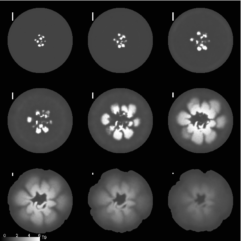
Figure 5: Snapshots of the temperature distribution in a meridian plane of model B30U at times from 0 to 1.3 s, in steps of $\sim 0.15$ s. The temperature scale is shown at the bottom left of the image, while the length scale is shown at the top left of each snapshot (the length of the vertical bar is equivalent to 200 km).

3.2 Comments on the numerical consistency of the calculations

The numerical noise present in the initial model must be as low as possible to not interfere with the rising of the hot elements, especially at the beginning, when they move very subsonically. For given initial conditions (i.e. number and size of ignited blobs) the evolution of the model is determined by the interplay between the Archimedean force and the effective combustion through the bubble surface. While the correct buoyancy can be reasonably reproduced by taking large enough bubbles and minimizing the numerical viscosity of the code, the effective combustion rate is hard to treat numerically. During their rising, the incinerated chunks of material are subjected to the Kelvin-Helmholtz and other hydrodynamical instabilities which greatly deform their geometry. Such deformation takes place in a range of scalelengths which can not be fully resolved by any present hydrocode neither in 3D nor in 2D. On the other hand, the increase of the bubble area competes with surface destruction due to the collision between the floating elements. It has been argued that these two antagonic effects give rise to a self-regulating mechanism which finally decouples the macroscopic burning velocity from the microphysics. Even though there are some indications that such a self-regulating mechanism could be at work during the development of the explosion (Khokhlov k95 (1995), Gamezo et al. gkochr03 (2003), García-Senz & Bravo gsb03 (2003)) its existence has not yet been proved. In this work, we have adopted a practical point of view by incorporating the effect of those scalelengths not resolved by the SPH simulation through a constant effective burning velocity that we called the baseline velocity, $v_{\mathrm{b}}$.

In the present models, we adopted a value of $v_{\mathrm{b}}=200$ km s^-1, which is similar to what can be found in current supernova literature. Due to the self-adjustment of the flame surface, the dependence of the outcome of the explosion on the particular value adopted for $v_{\mathrm{b}}$ is much weaker than that observed in one-dimensional models with respect to the parametrized burning front velocity. We have recalculated model B30U with a baseline velocity of 100 km s^-1 and have obtained variations in the released nuclear energy and ⁵⁶Ni mass of only 8%. Paradoxically, it was the smallest flame velocity run which burned most fuel and released most nuclear energy.

Of particular importance is the amount of spureous viscosity introduced by the hydrocode, because it could prevent the rise of hot blobs below a critical size. For example, for a small sphere subjected to an effective gravity, $g_{\mathrm{eff}}=g(\Delta\rho/\rho)$, the outward acceleration is given by: $a(r)=g_{\mathrm{eff}}(r)-F_{\mathrm{D}}(r)/m_{\mathrm{b}}(r)-F_{\mathrm{S}}(r)/m_{\mathrm{b}}(r)$, where $m_{\mathrm{b}}$ is the mass of the sphere, $F_{\mathrm{D}}$ is the drag force and $F_{\mathrm{S}}$ is the Stokes force induced by shear viscosity. A common expression used to calculate the drag force is $F_{\mathrm{D}}=0.5C_{\mathrm{D}}\rho v^{2}\pi R_{\mathrm{b}}^{2}$ (where $C_{\mathrm{D}}$ is the drag coefficient, of order unity). For an ascending sphere the Stokes force is given by $F_{\mathrm{S}}=6\pi\rho\nu R_{\mathrm{b}}v$, where $\nu$ is the kinematic viscosity coefficient and $v$ is the ascending velocity of the sphere relative to the surrounding fluid. Therefore $F_{\mathrm{D}}/m_{\mathrm{b}}\propto v^{2}/R_{\mathrm{b}}$ and $F_{\mathrm{S}}/m_{\mathrm{b}}\propto\nu v/R_{\mathrm{b}}^{2}$. In a white dwarf $\nu$ is very low and the Stokes force completely negligible. Nevertheless, the numerical viscosity introduced by any hydrocode is many orders of magnitude larger than the actual microscopic viscosity. Given the different dependence on $R_{\mathrm{b}}$ and $v$ shown in the previous expressions for $F_{\mathrm{D}}/m_{\mathrm{b}}$ and $F_{\mathrm{S}}/m_{\mathrm{b}}$, the numerical viscosity can introduce a non-negligible force during the first stages of the ignition phase, when the radius and the velocity of the burned blobs still remain small. For large enough blobs, the Stokes force rapidly becomes weaker than the drag force, and the numerical viscosity is not expected to interfere with the simulations. In SPH, one source of viscosity (although not the only one) is the artificial viscosity term devised to handle shock waves. Roughly, this term introduces an amount of viscosity $\nu\simeq\alpha hc_{\mathrm{s}}+\beta hv$ where $\alpha\simeq\beta\simeq 1$ are two parameters related to the linear and the quadratic terms present in the standard artificial viscosity formulation, and $c_{\mathrm{s}}$ is the local sound speed. Unfortunately, one can not choose $\alpha=\beta=0$ without compromising the stability of the initial model. We found that a reasonable choice is to take $\alpha=0,\leavevmode\nobreak\ \beta=1$, which, for our initial configuration of bubbles, leads to a Reynolds number of about five. As explained before, the procedure to set the initial conditions of our calculations ends with a brief hydrostatic episode of burning and heat conduction, until the flame around the blob is built. This strategy allows an increase in the size of the blobs, thus reducing the damping effect of the spurious numerical viscosity.

Figure 6: Radii of the centers of mass of the 30 bubbles of model B30U. The filled symbols over a line mark the time at which interaction with any other bubble first occurs.

Figure 7: Radial velocity of the bubbles as a function of the radii of their centers of mass, for model B30U.

3.3 Reference case: 30 bubbles

The evolution of the bubbles is governed by the competition between three processes:

• volume increase due to flame propagation and pressure equilibration with its surroundings,

• merging of bubbles, and

• surface deformation due to hydrodynamical instabilities.

We start by describing the evolution of model B30U (starting from 30 bubbles of nearly equal size), whose main trend can be seen in Figs. 5 to 11.

It takes about 0.3 s for the bubbles to start floating, from then on they follow an accelerated motion outwards to reach their terminal velocity before 1 s (Fig. 6). The final velocity of the bubbles ranges from 4 to $7.6\times 10^{8}$ cm s^-1(Fig. 7). Generally speaking, the bubbles that achieve the largest velocity are those whose initial locations are farther away from the center of the white dwarf, although there are exceptions. The deformation induced by the interaction among bubbles is a factor that feeds the hydrodynamic instabilities with a rich spectrum of scalelengths. This interaction among bubbles begins soon after runaway (Figs. 5 and 6). Rayleigh-Taylor mushrooms are well developed after a few tenths of a second, increasing the net fuel consumption rate, which peaks between 0.6 and 0.8 s, when the density of the bubbles has decreased below $10^{8}$ g cm^-3. The local flame velocity in each bubble (defined as $\left({\rm d}M_{\mathrm{b}}/{\rm d}t\right)/4\pi R_{\mathrm{b}}^{2}\rho_{\mathrm{b}}$) reaches its maximum at about the same time, and ranges from 400 to 700 km s^-1. At the last time represented in Fig. 5 the merging is so advanced that the bubbles have lost their individual identity and the nuclear ashes form a continuum medium, which is the main component in between radii $10^{8}$ and $5\times 10^{8}$ cm. The small wavelengths that were present at earlier times have by then erased, and the overall appearance of the hot region is dominated by 7-8 large plumes. The central zone of the exploding white dwarf is occupied by cold unburnt C-O rich matter.

The diversity in the history of the different bubbles shows up also in the evolution of their growth rates (Fig. 8). A small departure in the size of the bubbles at the beginning is translated into a large difference in their final mass. The peak in the fuel consumption rate of each bubble can range over factor of five (Fig. 9), the largest values being attained in those bubbles initially located at lower altitude. Close to the center, the effective gravity is proportional to the radius, which implies that the floatability is lower than that of the bubbles born at larger radius. On the other hand, all the bubbles are already big enough at the beginning of the hydrodynamical simulation for the Stokes and drag forces not to play an important role in their evolution. Thus, bubbles born far away from the center float earlier and grow faster in physical size, but not in mass, with respect to those born close to the center. The latter, in turn, can sustain their large fuel consumption rate during a long time, while they remain at high densities.

Figure 8: Masses of the bubbles in model B30U.

Figure 9: Fuel consumption rate of the bubbles, for model B30U.

The evolution of the averaged (over spherical shells) profiles of temperature and ash mass fraction is shown in Fig. 10. In spite of the large departure of the models from spherical symmetry, these averages still help to understand the evolution of the deflagration in our simulations. By looking at the temperature and composition plots, one can see that during the first 0.4 s the hot burnt region floats away from the center and spreads over a wide range of radii, while the amount of consumed fuel grows only moderately. At 0.6 s (long-dashed curve in Fig. 10) there is a sudden rise of the temperature and of the ash content, but it occurs halfway the total mass of the white dwarf. By 0.8 s (dot short-dashed line in Fig. 10) the combustion is also propagating inwards, where the density is higher. Finally, at the last time shown combustion has almost stopped and, at the same time, there has been a slight redistribution of the ashes towards larger radii.

Figure 10: Temporal evolution of temperature (top graph), and burnt mass fraction (bottom graph), for model B30U. The times shown are: 0 (solid line), 0.2, (dotted line), 0.4 (short-dashed line), 0.6 (long-dashed line), 0.8 (dot short-dashed line), and 1.0 s (dot long-dahsed line). The plotted quantities have been averaged over spherical shells.

The onset of the Rayleigh-Taylor instability, and its feedback on the flame behaviour around the surface of the bubbles can be appreciated from Fig. 11. It shows the ratio between the local flame velocity in each bubble and the Rayleigh-Taylor velocity in the nonlinear regime , $v_{\mathrm{RT}}=\int{g_{\mathrm{eff}}{\rm d}t}$, as a function of time. Three phases can be outlined from this figure. At early times ($t\la 0.1-0.2$ s) the flame propagation is not driven by the Rayleigh-Taylor instability, which shows up as a lack of correlation between the flame velocity and $v_{\mathrm{RT}}$. From this time up to $\sim 0.6-0.7$ s the velocity of the flame scales with the Rayleigh-Taylor velocity, and the ratio $v_{\mathrm{flame}}/v_{\mathrm{RT}}$ remains almost constant with a value within the range 0.07-0.14, depending on the bubble. This second phase is skipped by a few bubbles, those which stay closest to the center and which can be identified in Fig. 11 by having the largest ratios. Finally, at still later times the fuel consumption rate starts decreasing due to the drop in density, and the flame velocity decouples again from the developement of the Rayleigh-Taylor instability.

Figure 11: The time evolution of the ratio of the local flame velocity to the non-linear Rayleigh-Taylor velocity for each bubble of model B30U.

The final output of the explosion is given in Table 2, together with the rest of computed models. Model B30U has been followed for a long time after the end of the combustion phase of the explosion, to gain insight into the evolution of the ejecta until homology sets in. As can be seen in Table 2, this model was integrated over 19,000 hydrodynamical time steps, until a time $t_{\mathrm{last}}\sim 5,5$ hours. The explosion produced $0.43\leavevmode\nobreak\ M_{\odot}$ of ⁵⁶Ni, and the ejected material acquired a kinetic energy at infinity of $0.43\times 10^{51}$ ergs. Both quantities are within the ranges expected in a typical Type Ia supernova, although the kinetic energy is at the low end of the allowed range. The performance of the SPH code can be evaluated through its capability to conserve integral quantities such as energy, momentum and angular momentum (last three columns in Table 2). As can be seen, the momentum and angular momentum are, for practical purposes, perfectly conserved, but the code does not follow as efficiently the transformation of energy from one kind to another. The total energy is not exactly conserved, the amount of energy lost in the whole simulation being about the same as the (low) energy deposited in the bubbles at $t=0$, in the initial incineration of the particles to NSE (see last column of Table 1).

Table 2: Results of the hydrodynamical simulations.

Model	$E^{\mathrm{a}}$	$M\left({}^{56}\mathrm{Ni}\right)$	$t_{\mathrm{last}}$	$I$	$\Delta E^{\mathrm{b}}$	$\Delta p^{\mathrm{c}}$	$\Delta L^{\mathrm{d}}$
	($10^{51}$ erg)	($M_{\odot}$)	(s)	(Time steps)	($10^{51}$ erg)	($10^{9}\leavevmode\nobreak\ M_{\odot}\mathrm{cm\leavevmode\nobreak\ s}^{-1}$)	($10^{17}\leavevmode\nobreak\ M_{\odot}\mathrm{cm}^{2}\mathrm{s}^{-1}$)
B30U	0.43	0.43	19480.	19000	$-0.07$	$4\times 10^{-9}$	$2\times 10^{-6}$
B10U	0.05	0.24	1.05	1800	$-0.03$	$3\times 10^{-8}$	$10^{-9}$
B07U	$-$	0.21	12.17	6100	$-0.06$	$5\times 10^{-8}$	$6\times 10^{-9}$
B06U	$-$	0.19	9.11	4400	$-0.07$	$3\times 10^{-8}$	$5\times 10^{-9}$
B90R	0.45	0.44	2.20	5700	$-0.07$	$10^{-8}$	$4\times 10^{-9}$

• Final energy (gravitational+internal+kinetic) of the ejected mass at the last computed time, $t_{\mathrm{last}}$.

• Accumulated error in the total energy at the last computed model, after $I$ time steps.

• Total momentum at the last computed model, normalized taking as a characteristic velocity of the ejecta $10^{9}$ cm s^-1.

• Total angular momentum at the last computed model, normalized taking as a characteristic velocity of the ejecta $10^{9}$ cm s^-1, and a characteristic radius of $10^{8}$ cm.

3.4 Dependence on the number and size of the bubbles

The number of bubbles ignited at $t=0$ turns out to be a very influential parameter with respect to the evolution and final output of the explosion. From the results displayed in Table 2, two trends can be realised: First, for a small number of bubbles ($N_{\mathrm{b}}\la 30$) the quantity of ⁵⁶Ni produced and the amount of nuclear energy released grow with $N_{\mathrm{b}}$. Indeed, models B06U and B07U remained bound at the end of nuclear burning, and model B10U became only marginally unbound, but even in this case no more than a few percent of the mass of the white dwarf would be able to overcome the gravitational barrier. Nevertheless a word of caution must be given when the initial number of incinerated bubbles is low. In that case the use of a constant baseline velocity for the subgrid is less justified because the regulating mechanism based on flame surface self-adjustement does not work so well as in the case of a large number of bubbles displaying a larger surface. Thus, the critical number of igniting regions that might result in a successful explosion could be slightly different from what was obtained in our calculations. This point will be explored through a parameter study and reported in a forthcoming publication (Bravo & García-Senz 2005, in preparation). Second, for a larger number of bubbles ($N_{\mathrm{b}}\ga 30$) the explosion converges to a unified solution, and the output is quite insensitive to both the precise value of $N_{\mathrm{b}}$ and the size spectrum of the bubbles. Thus, models B30U and B90R give rise to almost the same explosion. This result is remarkable, as it marks the onset of convergence to an homogeneous supernova explosion, independently of the precise initial conditions. Recall that homogeneity is a primordial observational property of SNIa.

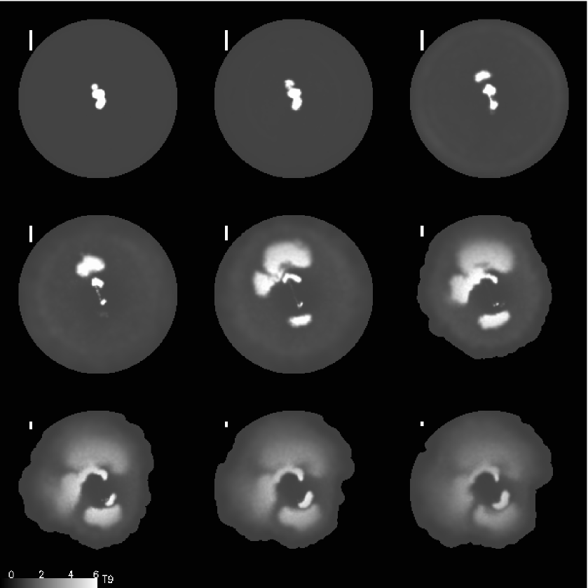
Figure 12: Snapshots of the temperature distribution in a meridian plane of model B07U at times from 0 to 1.05 s, in steps of $\sim 0.13$ s. The temperature scale is shown at the bottom left of the image, while the length scale is shown at the top left of each snapshot (the length of the vertical bar is equivalent to 200 km).

Figure 13: Snapshots of the temperature distribution in a meridian plane of model B90R at times from 0 to 1.10 s, in steps of $\sim 0.14$ s. The temperature scale is shown at the bottom left of the image and the length scale is shown at the top left of each snapshot (the length of the vertical bar is equivalent to 200 km).

In the following, we describe the main trends of models B07U and B90R, as representative of the two groups of models identified before. The evolution of both models is exemplified in Figs. 12 to 17.

It is worth comparing the thermal structure evolution of models B07U (Fig. 12) and B90R (Fig. 13) with that of model B30U (Fig. 5). The most evident difference between model B07U and the other two is the large departure from spherical symmetry of the first one. In B07U, there is a dominant bubble (the one located upwards in the picture), that grows fast, floats the most rapidly, and determines the overall evolution of the explosion. This can also be deduced from Fig. 14, which shows the fuel consumption rate of each bubble. The dominant bubble is subjected to hydrodynamic instabilities, and its surface is deformed sooner. The subsequent increase of flame surface largely compensates for the expansion effect on nuclear reactions. The dominant bubble reaches the outer layers of the white dwarf at $\sim 0.5-0.6$ s, when nuclear burning rapidly fades. The bubble then acts like a piston, pushing against the surrounding material, which provokes a break-out and the subsequent outflow of matter around the surface of the star.

In model B90R, in contrast, there is not one single bubble that dominates the fuel consumption rate (Fig. 15). In this model, not all the bubbles survive the first few tenths of a second after initial ignition, because most of them are ingested by the largest blobs. However, the overall evolution is quite similar to model B30U. The main difference between the evolution of B30U and B90R is that the latter displays a larger diversity of bubble sizes at any given time. This implies in turn a different floatability and, thus, a larger range of spatial scales present in the structure of the 90 bubbles model. Hence, the Rayleigh-Taylor mushrooms develop earlier, and the fine-scale structure is more complex at late times.

Figure 14: Fuel consumption rate of the bubbles for model B07U.

Figure 15: Fuel consumption rate of the bubbles, for model B90R.

The rate of nuclear binding energy released by all the bubbles, $\dot{\epsilon}_{\mathrm{nuc}}$, is depicted in Fig. 16 as a function of time, while the fuel consumption rate summed over all the bubbles is shown in Fig. 17 as a function of density. The temporal evolution of $\dot{\epsilon}_{\mathrm{nuc}}$ is similar for all the models, although the rate is noticeably smaller for the explosions which start from a small number of bubbles. On the other hand, the explosions starting from 30 and 90 bubbles differ only in the moment at which the maximum rate is attained; this is earlier in B90R by about 20% in time. Figure 17 shows how most of the fuel is burnt at moderate densities ($\rho_{\mathrm{b}}$ in the interval $2\times 10^{7}-2\times 10^{8}$ g cm^-3) in all the calculations.

Figure 16: Nuclear energy generation rate as a function of time. Solid line: model B30U, dashed line: model B90R, dotted line: model B7U.

Figure 17: Total fuel consumption rate as a function of density. Solid line: model B30U, dashed line: model B90R, dotted line: model B7U.

The long-term evolution of the models that fail to explode will be the subject of a forthcoming paper. In these models, the released energy will result in expansion followed by recontraction of the white dwarf. However, the chemical profile of the infalling matter will be quite different from what is inferred in current 1D pulsating delayed detonation models. Some hints of the possible outcome of such a situation have already been presented in Bravo & García-Senz (bgs04 (2004)).

3.5 Nucleosynthesis

The detailed nucleosynthesis produced in the successful explosions has been computed with a post-processing code. The results, which can be found in Table 3, reveal that models B30U and B90R produce virtually the same species and in the same quantities.

Table 3: Nucleosynthesis productivity, in solar masses.

	B30U	B90R		B30U	B90R
12C	0.282	0.276	55Mn	8.4E-4	8.0E-4
16O	0.387	0.389	54Fe	0.044	0.041
20Ne	0.027	0.027	56Fe	0.482	0.489
22Ne	0.010	0.010	57Fe	9.8E-3	0.010
24Mg	0.013	0.014	59Co	2.9E-4	3.0E-4
28Si	0.045	0.048	58Ni	0.046	0.043
32S	0.011	0.010	60Ni	0.023	0.023
36Ar	1.8E-3	1.4E-3	61Ni	4.8E-4	5.0E-4
40Ca	1.8E-3	1.3E-3	62Ni	1.4E-3	1.4E-3
44Ca	2.6E-5	2.6E-5	65Cu	3.5E-6	3.6E-6
48Ti	4.6E-5	4.3E-5	64Zn	4.3E-4	4.5E-4
52Cr	2.7E-4	2.2E-4	66Zn	3.7E-5	3.8E-5

The most salient nucleosynthetic feature is the large amount of unburnt C and O. As shown in Fig. 18, this C-O rich matter is present at any distance from the center of the ejecta, although it concentrates preferentially in the innermost and in the outermost layers. The presence of carbon and oxygen in the central layers of 3D deflagration models has sometimes been regarded as a failure of the pure deflagration scenario (Gamezo et al. gkochr03 (2003)), but it is not clear at all whether or not they would be actually detectable in current observations of SNIa (Baron et al. blh03 (2003)).

The isotopic composition of Fe-peak nuclei presents moderate excesses of ⁵⁴Fe, ⁵⁸Ni and ⁶⁰Ni. Our post-processing calculations start from an initial composition of 49% ¹²C, 49% ¹⁶O, and 2% ²²Ne. Further neutronization is provided by electron captures on NSE matter at high density. Basically, this affects the matter burned in the bubbles at the beginning of the hydrodynamical simulation (i.e. at $t=0$). The time scale for the decrease of the density of the bubbles is $\sim 0.3$ s, but in that time the mass of the bubbles hardly increases by a factor $\sim 2$ above its initial value (Fig. 8). The final electron molar number of the particles incinerated at $t=0$ reaches a value of $\sim 0.468$ mol g^-1, and the composition corresponding to freezing-out from NSE at this $Y_{\mathrm{e}}$ is dominated by the same neutronized nuclei as mentioned above, plus ⁵⁶Fe.

The amount of intermediate-mass elements (IME) ejected in the explosions is rather small (Table 3), and their distribution in velocity space is excessively smeared and too close to the center (Fig. 18) for a Type Ia supernova. Indeed, the presence of ⁵⁶Ni (⁵⁶Fe after the radioactive decays) in the external layers would produce quite distinctive spectral features near maximum, which remain undetected in SNIa so far. The scarcity in the production of IME could be in part related to the rough description of flame propagation at low densities ($\la 10^{7}$ g cm^-3), which is a weakness common to most 3D SNIa hydrocodes.

Figure 18: Final distribution of elements in velocity space. Top: model B30U, bottom: model B90R. The composition corresponds to the final products after radioactive disintegrations.

The worst flaw of the present models is the high degree of mixing of the elements in velocity space. The stratification of the ejecta is a feature strongly suggested by the observations, only allowing a moderate amount of mixing. The absence of such stratification in the models is a direct consequence of the formation of large plumes of ashes due to hydrodynamic instabilities. As strong radial mixing is a common feature of all 3D deflagration models computed by the astrophysical community (e.g. G03 and RHN), it casts serious doubts on the soundness of pure deflagrations as models of Type Ia supernovae.

As it is the result of a 3D simulation, one should not expect that the material is ejected with spherical symmetry. However, the distribution of Fe with respect to different directions of motion is quite symmetric (Fig. 19), showing a small departure from the average curve only in the high-velocity tail of one of the components of the velocity. Such a small asymmetry would hardly have any observable consequences. On the other hand, the distribution of elements in physical space is neither homogeneous nor symmetric (Fig. 20), especially that of ⁵⁶Ni which concentrates in a few large pockets. The possible relevance of this heterogeneous distribution of ⁵⁶Ni will be the subject of discussion in the next section.

Figure 19: Distribution of iron as a function of the components of the velocity, model B30U.

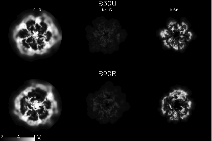
Figure 20: Final (at $t\sim 3$ s) chemical composition mapped onto a meridional plane, for models B30U (top row) and B90R (bottom row).

4 The long term evolution

The large computational cost of 3D hydrodynamical calculations is a factor that severely limits the time range explored in the simulations. Usually, 3D simulations of SNIa are followed for no more than 1-2 s, and the final model is expected to be representative of the final output of the thermonuclear explosion. Even though by that time the nuclear reactions have quenched and the chemical composition is already fixed, the density is still high and the dynamical interactions between different regions in the ejecta are able to change substantially the distribution of specific kinetic energy. With the aim to explore these effects, we have followed one of the succesful explosions (B30U) until an elapsed time of 19480 s (see Table 2). Our intention is to try to answer three fundamental questions in this section (within the limits imposed by the limited time we have been able to calculate):

• When do the ejecta achieve the homologous expansion phase?

• How can models be extrapolated from $\sim 1$ s up to times spanning several hours?

• What other effects become relevant for determining the ejecta structure at later times?

Figure 21: Mean of the fractional change in particles velocity with respect to its final velocity. A 5% difference is attained at $\sim 16$ s, and a 1% difference at $\sim 27$ s.

Figure 21 is intended to provide a quantitative answer to the first question. We have computed, for model B30U, the difference between the velocity of each particle in the last computed model and its velocity at different, earlier, times. The quantity depicted in the figure is the average of these differences averaged over all the particles. It can be seen that at $t=1$ s the velocities still have to change, in average, by almost 50% of their final value. This fractional change drops to $\sim 35$% at $t=3$ s, and to 10% at $t=12$ s, 99% of the final velocity, on average, is reached at $t=27$ s. These figures can be considered representative of any 3D SNIa model, although the precise values can change with the kinetic energy of the ejecta or with the mechanism of the explosion. Generally speaking, more energetic explosions evolve faster and arrive earlier at the homologous expansion phase. For instance, for an explosion twice as energetic as B30U, the mean velocity would scale as $2^{1/2}$, while the hydrodynamical time scale would change as $\rho^{-1/2}\propto R^{3/2}\propto v^{3/2}$, i.e. it would evolve $\sim 1.7$ times faster than B30U. Thus, the onset of the homologous expansion phase is expected to occur at times $\ga 16-30$ s.

Figure 22: Radius of each SPH particle at $t\sim 1$ s vs final radius, for model B30U.

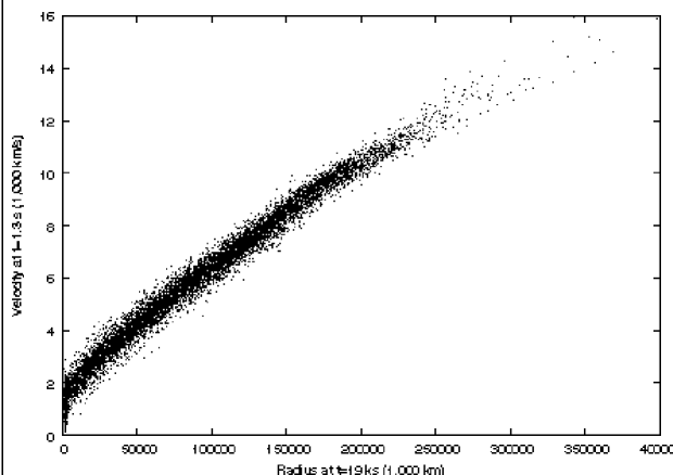
Figure 23: Velocity of each SPH particle at $t\sim 1$ s vs final radius, for model B30U.

Very often, 3D simulations cannot be extended much beyond $1-2$ s. In these cases, even though a detailed nucleosynthetic calculation can be performed, the final distribution of elements in velocity space remains uncertain. In principle, one has two ways to extrapolate the known distribution at early times in order to guess what the final chemical profile will be: either sorting the chemistry by radius, or by velocity (at $t\sim 1-2$ s, the homology relationship $v\propto r$ does not apply, as we have just seen). Figures 22 and 23 show the result of both kinds of extrapolation procedures compared to the actual distribution in the last computed model of B30U. The relevant quality of the distribution of points shown in those figures is its width. Wide distributions (like that in Fig. 22) are indicative of important changes in the ordering of the particles, while narrow ones point to a larger degree of conservation of the order. The conclusion is clear: sorting by velocity gives results much closer to the final situation than sorting by radius.

A hint of the reason why sorting by velocities gives better results can be sketched from inspection of Fig. 24. There, we have plotted the differential velocity of the bubbles with respect to their immediate surroundings as a function of time. Bubbles experience a strong acceleration due to buoyancy during the first $0.3-0.5$ s. During this period, the transfer of momentum to the surrounding material is small, hence the differential velocity of the bubbles rises steadily. During the next $\sim 0.2$ s, the outermost matter is accelerated by the bubbles, mainly due to the large increase in their lateral size, which makes radial transfer of momentum more efficient. Then, a short period of relative deceleration ensues, followed by a stabilization of the differential velocity. In this last phase the bubbles still move through the blobs of unburnt C-O, reaching farther regions and slowly transferring a fraction of their momentum to them.

Figure 24: Radial velocity of the bubbles relative to their environment, for model B30U.

As we have shown before, the NSE matter expelled in the explosion is mostly concentrated in several discrete pockets. The presence of Fe-rich knots in the outer regions of supernova remnants has already been confirmed in several cases, particularly in the remnant of the historical Type Ia SN1572. But the observed knots are much smaller than those found in our simulations (Fig. 20). Indeed, the presence of chemical inhomogeneities (clumps) in the photosphere of SNIa has been limited by the spectral analysis of Thomas et al. (tkbb02 (2002)). The basic argument is that the presence of huge clumps would modify the profile of the SiII absorption line depending on the line of sight, in contrast with the high degree of spectral homogeneity of typical SNIa. To remain compatible with the homogeneity of SNIa, Thomas et al. estimated that the area of the clumps should represent less than 10% of the area of the photosphere at the moment of maximum luminosity.

Even though we were not able to extend our hydrodynamical simulations until such late times ($\sim 15$ days), we have made a rough estimation of the clumpiness of the ejecta in the following way. We have assumed homologous expansion from the last computed model ($\sim 4.5$ hours) up to 15 days. Then we have calculated an approximate location of the photosphere, in a given observational direction, by assuming a constant opacity, $\kappa\sim 0.2$ cm²g^-1, and computed the column density of material from the surface inwards, until a prescribed optical depth ($\tau=2/3$) was reached. The results are displayed in Fig. 25, both for the column density of ⁵⁶Ni above the photosphere, and for the constant photospheric velocity curves (note that a ⁵⁶Ni column density of 3.3 means that all the material above the photosphere in that location and in the direction normal to the plane of the figure is pure ⁵⁶Ni). The velocity curves show a large degree of spherical symmetry, with a large velocity gradient towards the limb, due to the lower component of the velocity in the observer’s direction. The overall appearance is dominated by 4-5 large clumps of ⁵⁶Ni. We believe that this kind of configuration of ⁵⁶Ni clumps is common to all 3D pure deflagation models and, thus, makes this class of explosion mechanism difficult to reconcile with SNIa observations. A delayed detonation (DDT) could alleviate this problem by breaking the clumps when the detonation hits them. The simulation of delayed detonations in 3D is necessary to ascertain the ability of DDT models to improve the results obtained within the pure deflagration scenario.

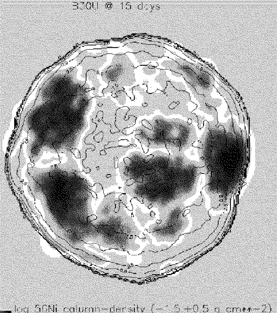
Figure 25: Column density of ⁵⁶Ni above the photosphere and contours of constant normal velocity at the photosphere, both for model B30U 15 days after the explosion.

Another effect we have not taken into account is the deposition of the radioactive energy into the ejecta, the so-called Ni-bubble effect. Depending on the size of the ⁵⁶Ni-rich bubbles, the gamma photons will be able or not to escape from the bubbles and deposit their energy either in their own bubble or in the surrounding matter. Thus, the Ni-bubble effect could make the problem of the clumps even worse by inducing additional expansion of the Ni-rich regions.

5 Conclusions

We have carried out hydrodynamical simulations and calculated the resulting nucleosynthesis of thermonuclear supernovae within the deflagration paradigm, starting from a few incinerated bubbles scattered through the central region of a white dwarf. This ignition scenario has recently received much attention from the supernova community, because it represents a more natural way of birth of the flame than the previously assumed ignition in a central volume. In this scenario, the evolution of the white dwarf has to be followed in 3D to avoid artificial solutions found previously in 2D calculations, as a consequence of symmetry impositions. The most recent 3D simulations to which our work can be compared are those from G03 and from the Munich group (e.g., RHN). In spite of the important differences in the computational procedure (SPH code in this work, PPM approach in G03 and in RHN), in the description of the flame (reaction-diffusion equation in our code and in G03, flame tracking through advection of a scalar quantity in RHN), in the maximum numerical resolution (20 km here, 2.6 km in G03, 3.33 km in RHN), in the precise initial conditions, and in the physics modules, the results of the different groups bear a close resemblance. The convergence of the gross features of the explosion picture gives us confidence that our simulations caught the fundamental properties of deflagrations in white dwarfs. The modest resolution attained in our calculations has allowed us to undertake a number of simulations that enlarge considerably the initial conditions explored so far. Moreover, in one case we have been able to follow the evolution of the explosion up to several hours after the thermonuclear burning stops.

The models starting from $\ga 30$ bubbles produced a healthy explosion of quite uniform characteristics, with nice amounts of ⁵⁶Ni and kinetic energy. However, the deformation of the flame surface during the first second of the explosion, owing to the inherent hydrodynamical instabilities, gave rise to important mixing of chemical elements through the ejecta. The absence of chemical stratification appears a serious problem of current 3D deflagration models of SNIa. Moreover, there are other drawbacks: an excessive mass of unburnt C-O, a large fraction of which moves at low velocity, close to the center of the ejecta, and the formation of large clumps of ⁵⁶Ni that show up at the photosphere near maximum brightness, in contrast with what the observational homogeneity of the SNIa sample suggests (Thomas et al. tkbb02 (2002)).

Nevertheless, the above models, characterized by a large number of bubbles ignited nearly-simultaneously, are not the only way a white dwarf can reach thermal runaway. Leaving aside the central ignition models, we have explored the possible initial configurations of igniting bubbles through a statistical analytical model. We have identified two extreme possibilities: a) a set of bubbles with almost equal size, and b) a set of bubbles of quite different dimensions whose number distribution is nearly independent of their size. The actual configuration that the white dwarf will have at runaway will depend on the degree of thermal homogeneity of the central region, $r\la 400$ km. If the thermal gradient around each hot spot is small enough, the configuration consisting of bubbles of equal size is preferred; otherwise, if the temperature changes by more than 1% in less than $\sim 100$ m, the second kind of configuration would be realised.

However, with respect to the results of the explosion, the only relevant parameter is the number of bubbles ignited at $t=0$. If this number is large enough ($\ga 30$ bubbles in the whole star or $3-4$ per octant), the explosion converges to the unified solution mentioned before. In contrast, if the number of igniting bubbles is scarce ($\la 2$ per octant) the explosion fails, and an oscillation of the white dwarf ensues. The final outcome of these oscillations, (if, for instance, they lead to a delayed detonation that could still produce a SNIa explosion) will be the subject of a forthcoming publication.

Appendix A Statistical approach to the initial distribution of igniting bubbles

The purpose of this appendix is to develop a statistical study of the size spectrum of the igniting bubbles located in the central region of a massive white dwarf at thermal runaway. Specifically, we try to determine the distribution function of the size, $R_{\mathrm{b}}$, of the igniting bubbles defined as the number of bubbles per unit size interval: $\phi\left(R_{\mathrm{b}}\right)\equiv{\rm d}N/{\rm d}R_{\mathrm{b}}$. This distribution function is itself a function of time. Our statistical approach is based on the following assumptions:

1. As a result of convection during the hydrostatic phase there appear several hot spots, which we assume to be spherically symmetric and initially chemically homogeneous. Instead of treating a hot spot as an isothermal sphere, we allow the temperature to be a function of distance to the center of the bubble, $R$. Each hot spot is then characterized by its central (peak) temperature, $T_{0}$, and its thermal profile.

2. Each hot spot evolves adiabatically in place, driven by its own nuclear energy generation rate, in a time given by its ignition timescale, $\tau_{\rm i}$. During this time, the temperature profile of the hot spot is modified due to the energy released by nuclear reactions, and to thermal conduction within the hot spot (see Fig. 1). For simplicity, we consider here that there is no interaction between different hot spots.

3. The statistical distribution of the initial peak temperatures of all the hot spots can be described by a continuous function, $\theta\left(T_{0}\right)$. The meaning of $\theta$ is the following: the number of hot spots whose peak temperature is inside the interval $\left[T_{0}:T_{0}+{\rm d}T_{0}\right]$ is given by ${\rm d}N=\theta\left(T_{0}\right){\rm d}T_{0}$. According to the above definitions, the desired distribution function of bubble radii is given by: $\phi\left(R_{\mathrm{b}}\right)=\theta\left(T_{0}\right)\left({\rm d}R_{\mathrm{b}}/{\rm d}T_{0}\right)^{-1}$. The dependence of the radius of the incinerated bubble at any time, $R_{\mathrm{b}}(t)$, on the initial peak temperature of the hot spot, $T_{0}$, is the main ingredient of our statistical approach.

We will work with two alternative distribution laws of the initial peak temperature of the hot spots, $\theta\left(T_{0}\right)$, either a gaussian or a linear law, both of which are defined in the interval from $T_{0}^{\mathrm{min}}$ to $T_{0}^{\mathrm{max}}$. Both distributions are decreasing functions of $T_{0}$ such that $\theta\left(T_{0}^{\mathrm{max}}\right)=0$. The gaussian distribution function is defined as:

$$\theta_{\mathrm{G}}\left(T_{0}\right)=2{{T_{0}^{\mathrm{max}}-T_{0}}\over{B^{\prime 2}}}{{\exp\left[-\left({{T_{0}^{\mathrm{m}ax}-T_{0}}\over{B^{\prime}}}\right)^{2}\right]}\over{{1-\exp\left[-\left({{T_{0}^{\mathrm{m}ax}-T_{0}^{\mathrm{min}}}\over{B^{\prime}}}\right)^{2}\right]}}};$$ (5)

where $B^{\prime}=10^{8}$ K is an arbitrary parameter. The linear distribution function is defined as:

$$\theta_{\rm L}\left(T_{0,8}\right)=\frac{T_{0}^{\mathrm{max}}-T_{0}}{2\times 10^{8}}\;,$$ (6)

where $T_{0,8}$ is $T_{0}$ in units of $10^{8}$K. In what follows, we use the values $T_{0}^{\mathrm{min}}=5\times 10^{8}$ K (the ignition timescale below this temperature becomes longer than 4h), and $T_{\rm 0}^{\mathrm{max}}=7\times 10^{8}$ K. Thus, once a particular $\theta$ has been chosen we only need to find the function $\left({\rm d}R_{\mathrm{b}}/{\rm d}T_{0}\right)$ to be able to determine $\phi$.

At densities $\rho\sim 2-3\times 10^{9}$ g cm^-3 the ignition timescale can be well approximated by $\tau_{\mathrm{i}}\left(T\right)\sim A\left(T/T_{\mathrm{b}}\right)^{-B}$, with $A=0.0193s$, $B=17.97$, and $T_{\mathrm{b}}=10^{9}\leavevmode\nobreak\ {\mathrm{K}}$ (cf. see Khokhlov k90 (1990), where it is called the induction time). For practical purposes, matter incinerates nearly instantaneously whenever its temperature exceeds $T_{\mathrm{b}}$. Central ignition of a hot spot occurs at a time $t=\tau_{\rm i}\left(T_{0}\right)-\tau_{\rm i}\left(T_{\mathrm{b}}\right)$ and thereafter the bubble will grow in mass and size. The first ignition of any hot spot is attained at a time $t=\tau_{\rm i}\left(T_{\rm 0}^{\mathrm{max}}\right)-\tau_{\rm i}\left(T_{\mathrm{b}}\right)$. As can be seen in Fig 2, the thermal profile of each individual bubble at central ignition (i.e. when the central temperature becomes equal to $T_{\mathrm{b}}$) can be fitted by a decreasing function of $R$:

$$T(R)=T_{\mathrm{b}}\exp\left[-\left(R/R_{0}\right)^{2}\right]\;,$$ (7)

where $R_{0}$ is a characteristic lengthscale.

Given the short timescales involved, there are only two mechanisms that can contribute to the growth of a bubble: conductive flame propagation and spontaneous flame propagation. One can expect that close to the center of the blob (large temperature, shallow gradients) spontaneous flame propagation will dominate, while far away conductive propagation will rule the flame. The transition radius from one mode to the other, $R_{\mathrm{tr}}$, is a parameter of the problem which basically depends on the assumed thermal profile around the blob center at the time of ignition.

During the spontaneous combustion phase, the ignition timescale at a distance $R$ from the center of a bubble is given by:

$$\tau_{\mathrm{i}}\left[T\left(R\right)\right]=\tau_{\rm i}\left(T_{\mathrm{b}}\right)\exp\left[B\left(R/R_{0}\right)^{2}\right]\;.$$ (8)

The phase velocity of the flame, $v_{\mathrm{sp}}=\left({\rm d}\tau_{\mathrm{i}}/{\rm d}R\right)^{-1}$, and the radius of a given bubble as a function of time can be easily obtained from the previous equation:

$$v_{\mathrm{sp}}\left(R\right)=\frac{R_{0}^{2}}{2B\tau_{\rm i}\left(T_{\mathrm{b}}\right)R}\exp\left[-B\left(\frac{R}{R_{0}}\right)^{2}\right]\;,$$ (9)

$$R_{\mathrm{b}}\left(t\right)=R_{0}\left\{\frac{1}{B}\ln\left[\frac{t-\tau_{\rm i}\left(T_{0}\right)+\tau_{\rm i}\left(T_{\mathrm{b}}\right)}{\tau_{\rm i}\left(T_{\mathrm{b}}\right)}\right]\right\}^{1/2}\;.$$ (10)

In the last equation, $\tau_{\rm i}\left(T_{0}\right)$ has to be evaluated at the value of $T_{0}$ (central temperature of a hot spot at $t=0$) that makes it possible that the radius of the bubble be equal to $R_{\mathrm{b}}$ at a time $t$. This is easily found to be:

$$T_{0}\left(R_{\mathrm{b}},t\right)=T_{\mathrm{b}}\left\{\frac{A}{t+\tau_{\rm i}\left(T_{\mathrm{b}}\right)-\tau_{\mathrm{i}}\left[T\left(R_{\mathrm{b}}\right)\right]}\right\}^{1/B}\;,$$ (11)

where $\tau_{\mathrm{i}}\left[T\left(R_{\mathrm{b}}\right)\right]$ is given by Eq. (A.4). Finally, after taking the derivative of $T_{0}$ with respect to $R_{\mathrm{b}}$, we arrive at the distribution function of the sizes of the bubbles during the spontaneous flame phase, as a function of time $t$:

$$\left(\frac{{\rm d}N}{{\rm d}R_{\mathrm{b}}}\right)_{\mathrm{sp}}=\frac{2T_{\mathrm{b}}\theta}{R_{0}^{2}}R_{\mathrm{b}}\frac{\exp\left[B\left(\frac{R_{\mathrm{b}}}{R_{0}}\right)^{2}\right]}{\left\{\frac{t}{A}+1-\exp\left[B\left(\frac{R_{\mathrm{b}}}{R_{0}}\right)^{2}\right]\right\}^{C}}\;,$$ (12)

with $\theta=\theta\left[T_{0}\left(R_{\mathrm{b}},t\right)\right]$, and $C={\left(B+1\right)/B}$.

The radius of transition from spontaneous combustion to conductive flame can be calculated as the radius at which the phase velocity given by Eq. (A.5) equals the laminar flame velocity, $v_{\mathrm{cond}}\approx 6.7\times 10^{6}$ cm s^-1 at the densities of interest. The results of this calculation can be seen in Fig. 26.

Figure 26: Radius of transition from spontaneous combustion to conductive flame as a function of the characteristic lengthscale of the thermal profile of the bubbles.

In our simplified picture, once a bubble attains the transition radius, the flame begins to propagate at the conductive velocity. As this conductive velocity is independent of the initial thermal profile of the hot spot, the distribution function of the bubbles of size $R_{\mathrm{b}}$ at time $t$ is the same as the distribution function at a size equal to the transition radius at the time $t-\Delta\left(R_{\mathrm{b}}\right)$, where $\Delta\left(R_{\mathrm{b}}\right)=\left(R_{\mathrm{b}}-R_{\mathrm{tr}}\right)/v_{\mathrm{cond}}$, i.e.,

$$\left(\frac{{\rm d}N}{{\rm d}R_{\mathrm{b}}}\right)_{\mathrm{co}}\left(R_{\mathrm{b}},t\right)=\left(\frac{{\rm d}N}{{\rm d}R_{\mathrm{b}}}\right)_{\mathrm{sp}}\left[R_{\mathrm{tr}},t-\Delta\left(R_{\mathrm{b}}\right)\right]\;.$$ (13)

The final results are shown in Figs. 3 and 4.

We have tested the sensitivity of the results to different assumptions about the thermal profile within the bubbles at ignition (eq. A.3), but we have not found any significant differences. The main limitations of our approach derive from the assumptions made in order to make the analytical calculation affordable. As discussed in more detail in Sect. 2 we have not considered changes in density during combustion, neither have we included heat transport by turbulence, which could influence the early phases of the ignition. During the first stage of bubble combustion following central ignition, dominated by spontaneous burning, there is no time for turbulence to contribute appreciably to the transport of thermal energy. Later on, conduction dominates but this is probably only true for small fluid elements where the ratio surface/volume is high. On the other hand, the statistical distribution of peak temperatures at t=0 s could be modified by turbulence before ignition. However, we have shown that the precise form of this statistical distribution is not relevant for the results of our analytical model.

References

- (1) Badenes, C. 2004, PhD Thesis, Universitat Politècnica de Catalunya
- (2) Baron, E., Lentz, E.J., & Hauschildt, P.H. 2003, ApJ, 588, L29
- (3) Bravo, E., & García-Senz, D. 2003, in From Twilight to Highlight: The physics of supernovae, ed. W. Hillebrandt, & B. Leibundgut (Berlin: Springer), 165
- (4) Bravo, E., & García-Senz, D. 2004, in Supernovae (10 years of SN1993J), eds. J.M. Marcaide, & K.W. Weiler, in press.
- (5) Cabezon, R.M., García-Senz D, & Bravo, E. 2004, ApJS, 151, 345
- (6) Gamezo, V.N., Khokhlov, A.M., Oran, E.S., Chtchelkanova, A.Y., & Rosenberg, R.O. 2003, Science, 299, 77 (G03)
- (7) García-Senz D., & Bravo, E. 2003, in From Twilight to Highlight: The physics of supernovae, ed. W. Hillebrandt, & B. Leibundgut (Berlin: Springer), 158
- (8) García-Senz D., Bravo, E., & Serichol, N. 1998, ApJS, 115, 119
- (9) García-Senz D., & Woosley, S.E. 1995, ApJ, 454, 895
- (10) Hatano, K., Branch, D., Lentz, E.J.,Baron, E., Filippenko, A.V., & Garnavich, P.M. 2000, ApJ, 543, L49
- (11) Höflich, P.A., & Stein, J. 2002, ApJ, 568, 779
- (12) Kasen, D., Nugent, P., Wang, L., Howell, D.A., Wheeler, J.C., Höflich, P., Baade, D., Baron, E., & Hauschildt, P.H. 2003, ApJ, 593, 788
- (13) Khokhlov, A.M. 1990, MPA Report number 513
- (14) Khokhlov, A.M. 1995, ApJ, 449, 695
- (15) Marion, Höflich, P., Vacca, W.D., & Wheeler, J.C. 2003, ApJ, 591, 316
- (16) Napiwotzki, R. et al. (SPY consortium) 2002, A&A, 386, 957
- (17) Niemeyer, J., Hillebrandt, W., & Woosley, S.E. 1996, ApJ, 471, 903
- (18) Nugent, P., Baron, E., Hauschildt, P., & Branch, D. 1997, ApJ, 485, 812
- (19) Reinecke, M., Hillebrandt, W., & Niemeyer, J. 2002, A&A, 391, 1167 (RHN)
- (20) Saio, H., & Nomoto, K. 1998, ApJ, 500, 388
- (21) Segretain, L., Chabrier, G., & Mochkovitch, R. 1997, ApJ, 481, 355
- (22) Thomas, R.C., Kasen, D., Branch, D., & Baron, E. 2002, ApJ, 567, 1037
- (23) Timmes, F.X., Hoffman, R.D., & Woosley, S.E. 2000, ApJS, 129, 377
- (24) Timmes, F.X., & Woosley, S.E. 1992, ApJ, 396, 649
- (25) Woosley, S.E., Wunsch, S., & Kuhlen, M., 2004, ApJ, 607, 921