Covariance of Weak Lensing Observables

Abstract

Analytical expressions for covariances of weak lensing statistics related to the aperture mass $M_{\rm ap}$ are derived for realistic survey geometries such as SNAP for a range of smoothing angles and redshift bins. We incorporate the contributions to the noise due to the intrinsic ellipticity distribution and the effects of finite size of the catalogue. Extending previous results to the most general case where the overlap of source populations is included in a complete analysis of error estimates, we study how various angular scales in various redshifts are correlated and how the estimation scatter changes with survey parameters. Dependence on cosmological parameters and source redshift distributions are studied in detail. Numerical simulations are used to test the validity of various ingredients to our calculations. Correlation coefficients are defined in a way that makes them practically independent of cosmology. They can provide important tools to cross-correlate one or more different surveys, as well as various redshift bins within the same survey or various angular scales from same or different surveys. Dependence of these coefficients on various models of underlying mass correlation hierarchy is also studied. Generalisations of these coefficients at the level of three-point statistics have the potential to probe the complete shape dependence of the underlying bi-spectrum of the matter distribution. A complete error analysis incorporating all sources of errors suggest encouraging results for studies using future space based weak lensing surveys such as SNAP.

1 Introduction

Detection of weak lensing signals by observational teams (e.g., Bacon, Refregier & Ellis 2000, Hoekstra et al. 2002, Van Waerbeke et al. 2000, and Van Waerbeke et al. 2002) has led to a new avenue not only in constraining the background dynamics of the universe but in probing the nature of dark matter and dark energy as well. To do so one compares observations with theoretical results obtained from simulations or analytical methods.

Often numerical simulations are employed which use ray-tracing techniques as well as line of sight integration of cosmic shear (e.g., Schneider & Weiss, 1988, Jarosszn’ski et al., 1990, Wambsganns, Cen & Ostriker, 1998, Van Waerbeke, Bernardeau & Mellier, 1999, and Jain, Seljak & White, 2000, Couchman, Barber & Thomas 1999) to test analytical calculations of cosmic shear. Of course simulations are being constantly updated to match upcoming surveys with broader sky coverage.

Analytical techniques too have made progress in understanding of shear induced by line-of-sight density inhomogeneities. Typically cosmological perturbation theory is employed at large angular scales (e.g., Villumsen, 1996, Stebbins, 1996, Bernardeau et al., 1997, Jain & Seljak, 1997, Kaiser, 1998, Van Waerbeke, Bernardeau & Mellier, 1999, and Schneider et al., 1998) while techniques based on the hierarchical ansatz provide a good match to simulation results at smaller angular scales (e.g., Fry 1984, Schaeffer 1984, Bernardeau & Schaeffer 1992, Szapudi & Szalay 1993, 1997, Munshi, Melott & Coles 1999, 1999a, 1999b). Ingredients for such calculations include Peacock & Dodds (1996)’s prescription (see Peacock & Smith (2000) for a more recent fit) for the evolution of the power spectrum or equivalently the two-point correlation function. Recent studies report an excellent agreement between analytical results and numerical simulations of weak lensing effects (Valageas 2000a & b; Munshi & Jain 2000 & 2001; Munshi 2000; Bernardeau & Valageas 2000; Valageas, Barber & Munshi 2004; Barber, Munshi & Valageas 2004; Munshi, Valageas & Barber 2004). One the other hand, one may also use halo models for specific purposes (e.g. Takada & Jain 2003).

In realistic survey scenarios, weak lensing signals are accompanied by various noises due to the intrinsic ellipticity distribution of galaxies, shot-noise due to the discreet nature of the source galaxies and finite volume effects due to finite survey size. A detailed analysis of these sources of noises was carried out by Munshi & Coles (2003) following Schneider et al. (1998). Recent studies by Valageas, Munshi & Barber (2004) have used such techniques to model errors in future surveys such as SNAP. It was also possible to study cross-correlation among various surveys using such a technique. Recent analysis by Munshi & Valageas (2004) showed that cross-correlation studies between two different surveys will have the potential to detect systematics associated with weak lensing measurements. In Munshi & Valageas (2004) we concentrated in dividing the source population into two non-overlapping subsamples. Generalising these studies here we are also able to probe estimation error associated with more than two different smoothing angular scales for same or different source redshift distributions. Besides the generalisation of our studies to three-point statistics means that we are able to probe the whole bi-spectrum and to use it to constrain theories of primordial non-Gaussianity or non-Gaussianity induced by gravitational clustering.

This paper is organised as follows: in section 2, a very brief introduction to our notations is provided. The window functions used in the rest of the paper are introduced along with a simple model of correlations hierarchy. In section 3, we take into account these realistic sources of noise to study the scatter associated with various estimators. Specific survey characteristics based on SNAP class experiments are assumed for such an analysis. In section 4 we check the validity of our results against numerical simulations for a range of redshift distributions and smoothing angular scales. We also investigate the dependence of two-point and three-point correlations on large-scale structures. Finally section 5 is left for a discussion of our results. Appendix A provides details of the analytical results used in the main sections.

2 Notations and Formalism

Any weak lensing effect $X$ smoothed over some angular radius $\theta_{s}$ and averaged over the redshift distribution of sources $n(z_{s})$ can be written in terms of the fluctuations of the density field as:

$$X=\int{\rm d}{\vec{\vartheta}}\;U_{X}({\vec{\vartheta}})\;\int_{0}^{\chi_{\rm max}}{\rm d}\chi\;\tilde{w}(\chi)\;\delta(\chi,{\cal D}{\vec{\vartheta}}),\;\;\;\mbox{with}\;\;\;\tilde{w}(\chi)=\frac{3\Omega_{\rm m}}{2}\int_{z}^{z_{\rm max}}{\rm d}z_{s}\;n(z_{s})\;\frac{H_{0}^{2}}{c^{2}}\;\frac{{\cal D}(\chi){\cal D}(\chi_{s}-\chi)}{{\cal D}(\chi_{s})}\;(1+z).$$ (1)

Here the redshift $z$ corresponds to the radial distance $\chi$ and ${\cal D}$ is the angular distance, ${\vec{\vartheta}}$ is the angular direction on the sky, $\delta(\chi,{\cal D}{\vec{\vartheta}})$ is the matter density contrast and hereafter we normalize the mean redshift distribution of the sources (e.g. galaxies) to unity: $\int{\rm d}z_{s}\;n(z_{s})=1$. We note $z_{\rm max}$ the depth of the survey (i.e. $n(z_{s})=0$ for $z_{s}>z_{\rm max}$). Here and in the following we use the Born approximation which is well-suited to weak-lensing studies: the fluctuations of the gravitational potential are computed along the unperturbed trajectory of the photon (Kaiser 1992). We also neglect the discrete effects due to the finite number of galaxies. They can be obtained by taking into account the discrete nature of the distribution $n(z_{s})$. This gives corrections of order $1/N$ to higher-order moments of weak-lensing observables, where $N$ is the number of galaxies within the circular field of interest. In practice $N$ is much larger than unity (for a circular window of radius 1 arcmin we expect $N\ga 100$ for the SNAP mission) therefore in this paper we shall work with eq.(1). The angular filter $U_{X}$ depends on the weak lensing observable one considers. For instance, the filter associated with the aperture-mass $M_{\rm ap}$ is (Schneider 1996):

$$U_{M_{\rm ap}}=\frac{\Theta(\vartheta<\theta_{s})}{\pi\theta_{s}^{2}}\;9\left(1-\frac{\vartheta^{2}}{\theta_{s}^{2}}\right)\left(\frac{1}{3}-\frac{\vartheta^{2}}{\theta_{s}^{2}}\right),$$ (2)

where $\Theta$ is a top-hat with obvious notations. The angular radius $\theta_{s}$ gives the angular scale probed by these smoothed observables. As described in Munshi et al. (2004), the cumulants of $X$ can be written in real space as:

$$\langle X^{p}\rangle_{c}=\int_{0}^{\chi_{\rm max}}\prod_{i=1}^{p}{\rm d}\chi_{i}\;\tilde{w}(\chi_{i})\int\prod_{j=1}^{p}{\rm d}{\vec{\vartheta}}_{j}\;U_{X}({\vec{\vartheta}}_{j})\;\;\xi_{p}\left(\begin{array}[]{l}\chi_{1}\\ {\cal D}_{1}{\vec{\vartheta}}_{1}\end{array},\begin{array}[]{l}\chi_{2}\\ {\cal D}_{2}{\vec{\vartheta}}_{2}\end{array},\dots,\begin{array}[]{l}\chi_{p}\\ {\cal D}_{p}{\vec{\vartheta}}_{p}\end{array}\right),$$ (3)

or equivalently we can write in Fourier space:

$$\langle X^{p}\rangle_{c}=\int_{0}^{\chi_{\rm max}}\prod_{i=1}^{p}{\rm d}\chi_{i}\;\tilde{w}(\chi_{i})\int\prod_{j=1}^{p}{\rm d}{\bf k}_{j}\;W_{X}({\bf k}_{\perp j}{\cal D}_{j}\theta_{s})\;\;\left(\prod_{l=1}^{p}e^{ik_{\parallel l}\chi_{l}}\right)\;\;\langle\delta({\bf k}_{1})\dots\delta({\bf k}_{p})\rangle_{c}.$$ (4)

We note $\langle..\rangle$ the average over different realizations of the density field, $\xi_{p}$ is the real-space $p-$point correlation function of the density field $\xi_{p}({\bf x}_{1},..,{\bf x}_{p})=\langle\delta({\bf x}_{1})..\delta({\bf x}_{p})\rangle_{c}$, $k_{\parallel}$ is the component of ${\bf k}$ parallel to the line-of-sight, ${\bf k}_{\perp}$ is the two-dimensional vector formed by the components of ${\bf k}$ perpendicular to the line-of-sight and $W_{X}({\bf k}_{\perp}{\cal D}\theta_{s})$ is the Fourier transform of the window $U_{X}$:

$$W_{X}({\bf k}_{\perp}{\cal D}\theta_{s})=\int{\rm d}{\vec{\vartheta}}\;U_{X}({\vec{\vartheta}})\;e^{i{\bf k}_{\perp}.{\cal D}{\vec{\vartheta}}},\;\;\;\mbox{whence}\;\;\;W_{M_{\rm ap}}({\bf k}_{\perp}{\cal D}\theta_{s})=\frac{24J_{4}(k_{\perp}{\cal D}\theta_{s})}{(k_{\perp}{\cal D}\theta_{s})^{2}}.$$ (5)

The real-space expression (3) is well-suited to models which give an analytic expression for the correlations $\xi_{p}$, like the minimal tree-model (Valageas 2000b; Bernardeau & Valageas 2002; Barber et al. 2004) while the Fourier-space expression (4) is convenient for models which give a simple expression for the correlations $\langle\delta({\bf k}_{1})..\delta({\bf k}_{p})\rangle_{c}$, like the stellar model (Valageas et al. 2004; Barber et al. 2004). In this article we shall use the latter stellar model defined by:

$$\langle\delta({\bf k}_{1})..\delta({\bf k}_{p})\rangle_{c}=\frac{\tilde{S}_{p}}{p}\;\delta_{D}({\bf k}_{1}+\dots+{\bf k}_{p})\;\sum_{i=1}^{p}\prod_{j\neq i}P(k_{j}),\;\;\;\mbox{with}\;\;\;\tilde{S}_{2}=1,$$ (6)

where $\delta_{D}$ is the Dirac distribution and $P(k)$ is the 3-d power-spectrum of the density fluctuations. The coefficients $\tilde{S}_{3},\tilde{S}_{4},..$ are closely related (and approximately equal) to the skewness, kurtosis, .., of the density field. Then, substituting eq.(6) into eq.(4) yields (Munshi et al. 2004):

$$\langle X^{p}\rangle_{c}=\tilde{S}_{p}\int_{0}^{\chi_{\rm max}}{\rm d}\chi\;\tilde{w}^{p}\int{\rm d}{\vec{\vartheta}}\;U_{X}({\vec{\vartheta}})\;I_{X}(\chi,{\vec{\vartheta}})^{p-1},\;\;\;\mbox{with}\;\;\;I_{X}(\chi,{\vec{\vartheta}})=\frac{1}{2}\int\frac{{\rm d}{\bf k}_{\perp}}{k_{\perp}^{2}}\;\frac{\Delta^{2}(k_{\perp},z)}{k_{\perp}}\;W_{X}({\bf k}_{\perp j}{\cal D}_{j}\theta_{s})\;e^{-i{\bf k}_{\perp}.{\cal D}{\vec{\vartheta}}}.$$ (7)

Here we introduced the power per logarithmic wavenumber $\Delta^{2}(k)=4\pi k^{3}P(k)$. Of course, these expressions generalize in a straightforward fashion for many-point cumulants. For instance, for two-point cumulants we obtain within this model:

$$\langle X_{1}^{p}X_{2}^{q}\rangle_{c}=\tilde{S}_{p+q}\int_{0}^{\chi_{\rm max}}{\rm d}\chi\;\tilde{w}_{1}^{p}\tilde{w}_{2}^{q}\int{\rm d}{\vec{\vartheta}}\;\left\{\frac{p}{p+q}\;U_{1}({\vec{\vartheta}})\;I_{1}(\chi,{\vec{\vartheta}})^{p-1}\;I_{2}(\chi,{\vec{\vartheta}})^{q}+\frac{q}{p+q}\;U_{2}({\vec{\vartheta}})\;I_{1}(\chi,{\vec{\vartheta}})^{p}\;I_{2}(\chi,{\vec{\vartheta}})^{q-1}\right\}.$$ (8)

These quantities describe the cross-correlations between two surveys or subsamples, which are refered to by the subscripts “i=1,2”. The source redshift distributions $n_{i}(z_{s})$ and the smoothing angles $\theta_{si}$ can be different, as well as the directions on the sky. However, in this paper we shall restrict ourselves to correlations between angular cells which are centered on the same direction. Then there is no need to add an angular shift to the expressions (2) and (5) of the filter functions. On the other hand, note that the signal would decrease for nonzero angular separations. In this article we shall consider both two-point and three-point cumulants. The latter contain valuable information about the bispectrum and can be used as a template for non-Gaussianity studies.

The weak lensing effects associated with different redshift bins or angular scales are correlated since their lines of sight probe the same density fluctuations at low $z$ (where they are largest). In order to measure these cross-correlations we define the cross-correlation coefficients $r_{pq}$ as:

$$r_{pq}=\frac{\langle X_{1}^{p}X_{2}^{q}\rangle_{c}}{\langle X_{1}^{p+q}\rangle_{c}^{p/(p+q)}\langle X_{2}^{p+q}\rangle_{c}^{q/(p+q)}}\;,\;\;\;\mbox{in particular}\;\;\;r_{11}=\frac{\langle X_{1}X_{2}\rangle_{c}}{\langle X_{1}^{2}\rangle_{c}^{1/2}\langle X_{2}^{2}\rangle_{c}^{1/2}}.$$ (9)

The quantities $r_{pq}$ correspond to the two-point cumulants $\langle X_{1}^{p}X_{2}^{q}\rangle_{c}$ normalized in such a way that most of the dependence on cosmology and gravitational dynamics cancels out. Thus, if the two subsamples are highly correlated we have $r_{pq}\simeq 1$ while $r_{pq}\simeq 0$ if they are almost uncorrelated. In a similar fashion we can generalize $r_{pq}$ to three-point objects $r_{pqs}$ as:

$$r_{pqs}=\frac{\langle X_{1}^{p}X_{2}^{q}X_{3}^{s}\rangle_{c}}{\langle X_{1}^{p+q+s}\rangle_{c}^{p/(p+q+s)}\langle X_{2}^{p+q+s}\rangle_{c}^{q/(p+q+s)}\langle X_{3}^{p+q+s}\rangle_{c}^{s/(p+q+s)}}\;,\;\;\;\mbox{in particular}\;\;\;r_{111}=\frac{\langle X_{1}X_{2}X_{3}\rangle_{c}}{\langle X_{1}^{3}\rangle_{c}^{1/3}\langle X_{2}^{3}\rangle_{c}^{1/3}\langle X_{3}^{3}\rangle_{c}^{1/3}}.$$ (10)

These objects provide valuable information about the bi-spectrum as they directly probe three different angular scales over three different redshift distributions. They can also be used to study cross-correlations among three different surveys some of which may have overlapping source distributions. However note that as a result of subdividing the same source samples into various redshift bins the shot-noise will increase. In addition, being a true three-point object it will be more affected by the finite size of the survey volume at larger angular scales. However a good sky coverage for future surveys such as SNAP will mean these objects can be measured over reasonable angular length scales. It is possible to investigate even higher numbers of points (samples) but we shall not consider this here.

3 Future Surveys

3.1 A specific case study: Wide SNAP survey

In order to illustrate the measurements one can expect from future surveys, we consider here the case of the Wide SNAP survey. We use the characteristics of the SNAP mission as given in Refregier et al. (2004). The redshift distribution of galaxies and the total surface density $n_{g}$ of usable galaxies are:

$$n(z_{s})\propto z_{s}^{2}\;e^{-(z_{s}/z_{0})^{2}}\;\;\mbox{with}\;\;z_{0}=1.13,\;\;z_{\rm max}=3\;\;\;\mbox{and}\;\;\;n_{g}=100\;\mbox{arcmin}^{-2}.$$ (11)

The shear variance due to intrinsic ellipticities and measurement errors is $\sigma_{*}=\langle|\epsilon_{*}|^{2}\rangle^{1/2}=0.31$ while the survey covers an area $A=300\;\mbox{deg}^{2}$. Therefore, we take for the number $N$ of galaxies within a circular field of radius $\theta_{s}$ and for the number $N_{c}$ of cells of radius $\theta_{s}$:

$$N=n_{g}\pi\theta_{s}^{2}\simeq 314\left(\frac{n_{g}}{100\mbox{arcmin}^{-2}}\right)\left(\frac{\theta_{s}}{1\mbox{arcmin}}\right)^{2}\;\;\;\mbox{and}\;\;\;N_{c}=\frac{A}{(2\theta_{s})^{2}}=2.7\times 10^{5}\left(\frac{A}{300\mbox{deg}^{2}}\right)\left(\frac{\theta_{s}}{1\mbox{arcmin}}\right)^{-2}.$$ (12)

For some purposes we shall also consider the two subsamples which can be obtained from the Wide SNAP survey by dividing galaxies into two redshift bins: $z_{s}>z_{*}$ (which we refer to as “Wide$>$”) and $z<z_{*}$ (“Wide$<$”). We choose $z_{*}=1.23$, which corresponds roughly to the separation provided by the SNAP filters and which splits the Wide SNAP survey into two samples with the same number of galaxies (hence $n_{g}=50$ arcmin^-2).

For the background cosmology we consider a LCDM model with $\Omega_{\rm m}=0.3$, $\Omega_{\Lambda}=0.7$, $H_{0}=70$ km/s/Mpc and $\sigma_{8}=0.88$.

3.2 Two-point correlations for $M_{\rm ap}$

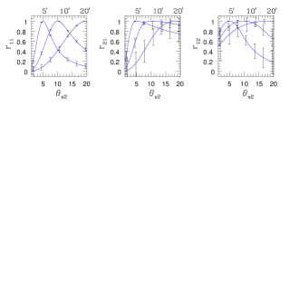
Figure 1: Correlation coefficients $r_{11}$ (left panel), $r_{21}$ (middle panel) and $r_{12}$ (right panel) are plotted as a function of the smoothing angle $\theta_{s2}$. All cases correspond to the full SNAP survey. The three different curves correspond to the smoothing angle $\theta_{s1}=5^{\prime},10^{\prime}$ and $20^{\prime}$, whereas $\theta_{s2}$ runs from $1^{\prime}$ to $20^{\prime}$. Errorbars associated with each curve show the 1-$\sigma$ scatter in the measured values, due to intrinsic ellipticities and cosmic variance.

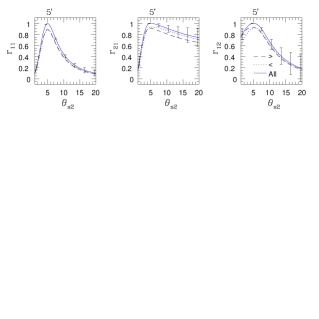
Figure 2: Correlation coefficients $r_{11}$, $r_{21}$ and $r_{12}$ are plotted for the wide SNAP survey with redshift binning. Solid curves denote the complete source sample whereas other line-styles correspond to redshift binning. The dashed curve “$>$” shows the case where $M_{\rm ap1}$ at fixed $\theta_{s1}$ is measured from high-$z$ galaxies ($z_{s1}>1.23$) while $M_{\rm ap2}$ at $\theta_{s2}$ which runs from $1^{\prime}$ to $20^{\prime}$ is measured from low-$z$ galaxies ($z_{s2}<1.23$). The dotted curve “$<$” corresponds to $z_{s1}<1.23$ and $z_{s2}>1.23$.

In this article we shall restrict ourselves to the statistics obtained from the aperture-mass $M_{\rm ap}$, defined from the filters $U_{M_{\rm ap}}$ and $W_{M_{\rm ap}}$ given in eqs.(2), (5). We first show in Fig. 1 the lowest-order two-point correlation coefficients $r_{pq}$ obtained at a fixed smoothing angle $\theta_{s1}$ while $\theta_{s2}$ runs from $1^{\prime}$ up to $20^{\prime}$, for the full wide SNAP survey. The three curves in each panel correspond to $\theta_{s1}=5^{\prime},10^{\prime}$ and $20^{\prime}$. The error-bars take into account the cosmic variance and the intrinsic ellipticities of galaxies, see Appendix and Munshi & Valageas (2004).

The correlation coefficients $r_{pq}$ show a peak where both scales coincide and are fully correlated ($r_{pq}=1$ as $M_{\rm ap1}$ and $M_{\rm ap2}$ are actually identical at this point). We find from $r_{11}$ that the correlation remains strong ($\ga 0.4$) up to an angular scale $\theta_{s2}$ twice larger than the other smoothing scale $\theta_{s1}$. We must point out that this depends on the smoothing window and that top-hat windows (for the smoothed convergence $\kappa_{s}$, or the shear components $\gamma_{i{\rm s}}$) generate more extended correlation profiles. This is related to the fact that the aperture-mass $M_{\rm ap}$ is a very localized filter in Fourier space (Schneider 1996). However, we can see that the third-order correlations $r_{21}$ and $r_{12}$ decrease much more slowly (especially $r_{21}$). It is interesting to note that the shapes of $r_{21}$ and $r_{12}$ are not identical and that $r_{21}$ exhibits in particular a very extended tail at larger angles. This can be understood from eq.(4). The Dirac factor $\delta_{D}({\bf k}_{1}+{\bf k}_{2})$ contained in the mean $\langle\delta({\bf k}_{1})\delta({\bf k}_{2})\rangle_{c}$ involved in $r_{11}$ implies $k_{1}=k_{2}$ so that $r_{11}$ peaks at $\theta_{s1}=\theta_{s2}$ where both $W(k_{1}{\cal D}\theta_{s1})$ and $W(k_{2}{\cal D}\theta_{s2})$ can be simultaneously maximized. Then, $r_{11}$ decreases for different angular scales where one cannot simultaneously maximize $W(k_{1})$ and $W(k_{2})$. On the other hand, for the third-order correlation $r_{21}$ the Dirac factor is $\delta_{D}({\bf k}_{1}+{\bf k}_{1}^{\prime}+{\bf k}_{2})$ with a weight $W(k_{1}{\cal D}\theta_{s1})W(k_{1}^{\prime}{\cal D}\theta_{s1})W(k_{2}{\cal D}\theta_{s2})$. Then, at large $\theta_{s2}$ it is still possible to maximize all three weights $W$ by choosing $k_{2}\sim 1/{\cal D}\theta_{s2}$, $k_{1}\sim k_{1}^{\prime}\sim 1/{\cal D}\theta_{s1}\gg k_{2}$, with ${\bf k}_{1}^{\prime}\simeq-{\bf k}_{1}$ and ${\bf k}_{2}=-{\bf k}_{1}-{\bf k}_{1}^{\prime}$. This is not possible for $r_{12}$ where the weight is now $W(k_{1}{\cal D}\theta_{s1})W(k_{2}{\cal D}\theta_{s2})W(k_{2}^{\prime}{\cal D}\theta_{s2})$ and from two small wavenumbers $k_{2}$ and $k_{2}^{\prime}$ of order $1/{\cal D}\theta_{s2}$ it is impossible to construct a wavenumber ${\bf k}_{1}=-{\bf k}_{2}-{\bf k}_{2}^{\prime}$ which is much larger ($k_{1}$ is of order $1/{\cal D}\theta_{s2}\ll 1/{\cal D}\theta_{s1}$). A similar reasoning also explains the steep decline of the correlation coefficient $r_{21}$ at low angular scales $\theta_{s2}$. Thus, the correlation coefficients $r_{pq}$ directly probe the features of the matter density field (note that the previous arguments only depend on the statistical homogeneity of the density field). We can see from Fig. 1 that the error-bars expected from the wide SNAP survey are quite small for $r_{11}$. They are larger for the third-order statistics $r_{21}$ and $r_{12}$ but one should still be able to obtain a good measure of the shape of these correlations. On the other hand, the measure of the coefficients $r_{pq}$ can provide a way to check the importance of noise and systematics.

Next, we show in Fig. 2 the effect of the redshift binning of the data. We divide the galaxies into two different bins: $z_{s1}>1.23$ and $z_{s2}<1.23$ (dashed curve “$>$”) or $z_{s1}<1.23$ and $z_{s2}>1.23$ (dotted curve “$<$”). Of course, the behaviour of the various correlation coefficients $r_{pq}$ remains similar to the case of only one redshift bin displayed in Fig. 1. However, at the peak $\theta_{s1}=\theta_{s2}$ we now have $r_{pq}<1$ since even for the same smoothing angle the quantities $M_{\rm ap1}$ and $M_{\rm ap2}$ are not identical as their lines of sight extend to different redshifts. Of course the error-bars are somewhat larger when we apply such a redshift binning of the data but it is still possible to measure these coefficients to a reasonable accuracy up to third-order statistics $r_{21}$ and $r_{12}$. This probes the evolution with redshift of gravitational clustering, although the latter is best measured with one-point statistics (most of the time dependence of the amplitude of density fluctuations and of the cosmological distances associated with various source redshifts is factorized out of the coefficients $r_{pq}$).

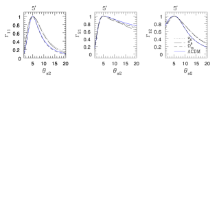
Figure 3: Correlation coefficients $r_{11}$, $r_{21}$ and $r_{12}$ are plotted for various cosmological or survey parameters. The solid line is our baseline LCDM model, the “$\Omega_{\rm m}$” curve shows a $20\%$ increase of $\Omega_{\rm m}$ (from $\Omega_{\rm m}=0.3$ up to $\Omega_{\rm m}=0.36$), the “$\sigma_{8}$” curve is a $20\%$ increase of $\sigma_{8}$ (from $\sigma_{8}=0.88$ up to $\sigma_{8}=1.06$) and the “$z_{0}$” curve is a $20\%$ decrease of the characteristic redshift $z_{0}$ of the survey (from $z_{0}=1.13$ down to $z_{0}=0.9$), eq.(11). The distance between these latter curves and the baseline model has been multiplied by a factor 20 since the dependence on cosmological or survey parameters actually nearly cancels out.

Finally, we also display in Fig. 3 the results obtained with a $20\%$ increase of $\Omega_{\rm m}$ (from $\Omega_{\rm m}=0.3$ up to $\Omega_{\rm m}=0.36$), or a $20\%$ increase of the normalization $\sigma_{8}$ of the density power-spectrum (from $\sigma_{8}=0.88$ up to $\sigma_{8}=1.06$), or a $20\%$ decrease of the characteristic redshift $z_{0}$ (eq.(11)) of the survey (from $z_{0}=1.13$ down to $z_{0}=0.9$). The distance between these latter curves and the baseline model (solid line) has been multiplied by a factor 20. Thus we see that the dependence on cosmological or survey parameters almost completely cancels out of the reduced correlation coefficients $r_{pq}$. Therefore, these quantities provide a direct handle on the noise or on the detailed properties of the large-scale density field (e.g. the validity of a hierarchical model like (6) for many-body correlation functions). On the other hand, cosmological parameters may be measured from one-point cumulants. Thus, the use of one-point, two-point and three-point cumulants provides a convenient separation between various features of the problem: cosmology, large-scale structures and noise.

3.3 Three-point correlations for $M_{\rm ap}$

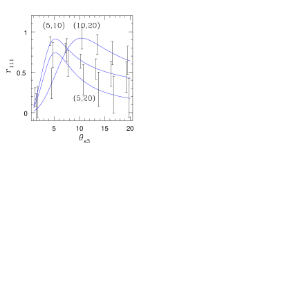
Figure 4: The correlator $r_{111}$ for the full wide SNAP survey is plotted as a function of smoothing angle $\theta_{s3}$ for a fixed pair of $(\theta_{s1},\theta_{s2})$. The pair $(\theta_{s1},\theta_{s2})$ for each curve is indicated in the plot. Error bars denote the $1-\sigma$ scatter around the mean.

We show in Fig. 4 the three-point correlation coefficient $r_{111}$ defined in eq.(10), for the full wide SNAP survey. This three-point object is a direct probe of the underlying bi-spectrum of the matter density field. The error-bars are computed from the expressions derived in the Appendix where the optimised estimators $H_{pqs}$ are used (this helps to reduce the scatter, see Valageas et al. 2004). The statistic $r_{111}$ is a symmetric function of its arguments when the three source redshift distributions are the same as in Fig. 4 where the full source sample is used. Then, when two smoothing angles are equal it coincides with the two-point statistics $r_{21}$ or $r_{12}$. As in the case of two-point correlators the error-bars are dominated by the finite size of the survey and are higher for larger smoothing angular scales. However from the figure we can see that SNAP will be able to probe $r_{111}$ reasonably well even when a large smoothing angle $\theta_{s2}=20^{\prime}$ or $\theta_{s3}=20^{\prime}$ is used. Redshift binning can be useful in studying the redshift evolution of $r_{111}$ but this reduces the number of sources thereby increasing the shot noise which starts playing a dominant role at smaller smoothing angular scales. The noise level at given smoothing angular scales is not only determined by the signal-to-noise ratios $\rho_{1}$, $\rho_{2}$ and $\rho_{3}$ of the variance of the aperture-mass at each scale but also by the overlap of various smoothing patches as described by $\rho_{12}$, $\rho_{23}$ and $\rho_{13}$, see eq.(20) and the Appendix. It is possible to generalise our results to cases where the patches are not all centered on the same line of sight but we shall not investigate this point here.

In Fig. 4 we plot $r_{111}$ for three combinations of $(\theta_{s1},\theta_{s2})$ while $\theta_{s3}$ runs from $1^{\prime}$ to $20^{\prime}$. The curves show a single peak reached when $\theta_{s3}$ is equal to the smallest angular scale among $(\theta_{s1},\theta_{s2})$. This may be understood as follows. Let $\theta_{s1}<\theta_{s2}$, then as $\theta_{s3}$ increases from $0^{\prime}$ the value of $r_{111}$ grows as the surface which is common to the three patches increases as $\theta_{s3}^{2}$. More to the point, the relative importance of the common surface increases: relative to the three quantities $M_{{\rm ap}j}$ it goes as $\{(\theta_{s3}/\theta_{s1})^{2},(\theta_{s3}/\theta_{s2})^{2},1\}$. Next, as $\theta_{s3}$ gets larger than $\theta_{s1}$ the common surface sticks to $\theta_{s1}^{2}$ (it no longer grows) while the relative common surface actually decreases as $\{1,(\theta_{s1}/\theta_{s2})^{2},(\theta_{s1}/\theta_{s3})^{2}\}$. Therefore, one can expect a steady decline beyond $\theta_{s1}$. This is indeed what we observe in Fig. 4. Of course, matters are actually a bit more intricate as the three-point correlation is not “$\delta_{D}$-correlated” in real space so that the correlation between different patches is not strictly proportional to their geometrical overlap and the filters $U_{M_{\rm ap}}$ are not simple top-hats. However, these simple arguments explain the overall trends seen in Fig. 4.

As expected, for a fixed angle $\theta_{s1}$ (here $5^{\prime}$) the peak of $r_{111}$ at $\theta_{s3}=\theta_{s1}$ is larger when $\theta_{s2}$ is closer to $\theta_{s1}$ (here $10^{\prime}$ as compared with $20^{\prime}$). Note that $r_{111}=1$ for $\theta_{s1}=\theta_{s2}=\theta_{s3}$ where the three quantities $M_{\rm ap1}$, $M_{\rm ap2}$ and $M_{\rm ap3}$ are identical whence fully correlated (for identical source distributions). We can see that the correlation of third-order statistics remains significant over a large range of angular scales and shows a slow decline at high $\theta_{s3}$ and a steeper falloff at low $\theta_{s3}$, in a fashion similar to $r_{21}$ shown in Fig. 1, for the same reasons.

4 Comparison with numerical simulations

We have shown in the previous section that the two-point and three-point correlators $r_{pq}$ and $r_{pqs}$ associated with the aperture-mass $M_{\rm ap}$ could be measured in future surveys like SNAP and allow a clean separation between cosmological parameters and the properties of the density field (the behaviour of its many-body correlations). They can also be used to monitor the noise of the survey. In this section, we address the use of these correlation coefficients from the point of view of large-scale structures. Thus, we first compare our predictions from the simple hierarchical model (6) with the results of numerical simulations. Secondly, we investigate the dependence of these correlators on the detailed properties of the density field.

The numerical method for the computation of the lensing statistics is based on the original formalism of Couchman, Barber & Thomas (1999) which concentrates on computation of three-dimensional shear matrices along lines of sight through the linked simulation volumes. This technique has been further developed by Barber (2002). This procedure which has been described in various publications in detail (e.g. Barber 2002) has been applied to a LCDM cosmological simulation created by the Hydra Consortium using the ‘Hydra’ $N$-body hydrodynamics code (Couchman, Thomas & Pearce, 1995). Its cosmological parameters are: $\Omega_{\rm m}=0.3$, $\Omega_{\Lambda}=0.7$, $\Gamma=0.25$, $H_{0}=93$ km/s/Mpc and $\sigma_{8}=1.22$. The computations of correlation functions were done by using concentric annuli which are divided in equal radial bins and angular bins in real space directly from the rectangular grid. Various combinations of bin width in radial and angular directions were considered while computing the correlations to check the stability of our scheme. Several levels of dilution were tested by increasing the grid size of the parent rectangular. For simplicity, we consider Dirac delta distributions of sources. That is, for three-point correlators all sources are located at the three redshifts $z_{s1},z_{s2}$ and $z_{s3}$ which can be different.

4.1 Two-point correlators

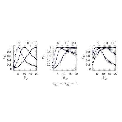
Figure 5: The two-point correlation coefficients $r_{11},r_{21}$ and $r_{12}$ are plotted for various angular scales. In each plot the curves from left to right correspond to $\theta_{s1}=5^{\prime},10^{\prime}$ and $20^{\prime}$, while $\theta_{s2}$ runs from $1^{\prime}$ to $20^{\prime}$. Source redshift is fixed at $z_{s1}=z_{s2}=1$. Solid points are measurements from simulation data while the solid curve is the theoretical prediction from the simple stellar model (6). Error-bars are computed from $10$ identical realizations. Note that the LCDM cosmology used for the simulations is slightly different from the one used for the SNAP survey.

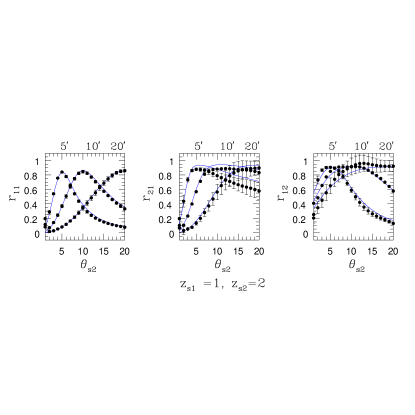
Figure 6: The two-point correlation coefficients $r_{11},r_{21}$ and $r_{12}$ are plotted for the angular scale $\theta_{s1}=5^{\prime},10^{\prime}$ and $20^{\prime}$ while $\theta_{s2}$ runs from $1^{\prime}$ to $20^{\prime}$. The redshift slices considered are $z_{s1}=1$ and $z_{s2}=2$. The solid curve is the analytical model (6) while solid points are measurements from simulation data.

We again study the two-point objects such as $r_{pq}$ by keeping one angular scale fixed, say $\theta_{s1}$, while the other smoothing angle $\theta_{s2}$ varies from $1^{\prime}$ to $20^{\prime}$ (unless $p=q$ and $z_{s1}=z_{s2}$, $r_{pq}$ is not a symmetric function of its arguments $\theta_{s1}$ and $\theta_{s2}$). This range is determined by the finite resolution of the simulations: smaller scales are affected by the rectangular grid (i.e. resolution) while large angular scales are affected by the finite simulation box. Note that effects due to the finite size of the box will be more prominent at smaller redshifts while effects due to the grid play a more important role at larger redshifts. In most of our studies we analyse cross-correlations and auto-correlations of various redshift slices against the slice $z_{s}=1$ which is least affected by such artifacts and of great observational interest.

We display the case of identical source redshifts $z_{s1}=z_{s2}=1$ in Fig. 5 and the case of different source redshifts in Fig. 6, with $z_{s1}=1$ and $z_{s2}=2$. As in Figs. 1, 2, the two-point correlators always show a peak where both angular scales coincide and complete overlap is achieved to generate a high correlation coefficient $r_{pq}$. Again, in cases where the same redshift slices are used for the two smoothing angles the coefficients $r_{pq}$ reach a value of unity, whereas for different redshift slices the maximum is less than unity as only partial overlap of the lines of sight is achieved. We also recover the slow decrease at large angles $\theta_{s2}$ of $r_{21}$. We can see that the simple hierarchical model (6) agrees reasonably well with the numerical simulations, although there is a small discrepancy at large angles $\theta_{s2}$ for $r_{21}$. However, the error-bars in this domain are large. In agreement with the nearly total independence of these correlation coefficients onto cosmology, described in Fig. 3, we have checked that an OCDM simulation (again from the Hydra Consortium) yields the same results. The error-bars shown are computed from a large number of realizations $n_{{\rm real}}=10$. As expected they are larger for higher-order statistics ($r_{21}$ and $r_{12}$ as compared with $r_{11}$). However, note that all realizations we have used are actually constructed from the same N-body density field and are not completely independent so there could be a systematic deviation (although expected to be small) in our results which can only be studied by using completely different simulations where density fields probed by various lines of sights are completely independent. In this article we only consider angular windows with zero separation. Then the scatter is mostly determined by the largest of the smoothing angles which defines how many independent patches there are for correlation studies.

The effects of small box size not only appear as an increased scatter for the estimation of high-order correlation functions it can also bias the mean. Detailed schemes exist in case of galaxy clustering to correct or estimate such bias from galaxy surveys or simulated catalogs. For large smoothing angles with $\theta_{s2}=20^{\prime}$ it is expected that such effects will be visible in the computed values of $r_{12}$ estimated from our simulated maps as there are only few independent patches within the survey and $r_{12}$ puts more weight on $\theta_{s2}$ as compared with $r_{21}$. Clearly such effects will be more pronounced at larger $\theta_{s1}$ and at lower redshifts where gravitational clustering has effectively generated correlated patches on the sky. We have made no attempt to correct for such a deviation. However, note that the compensated filter associated with $M_{\rm ap}$, which is very localized in Fourier space, makes these problems less acute than for simple tophat filters.

4.2 Three-point correlators

Figure 7: The three-point correlation coefficient $r_{111}$ as a function of smoothing angle $\theta_{s3}$ for a fixed pair of $(\theta_{s1},\theta_{s2})$. The pair $(\theta_{s1},\theta_{s2})$ for each curve is indicated in the plot. The three source redshifts are equal: $z_{s1}=z_{s2}=z_{s3}=1$. The solid curve is the analytical model (6) while solid points with error-bars are measurements from simulation data.

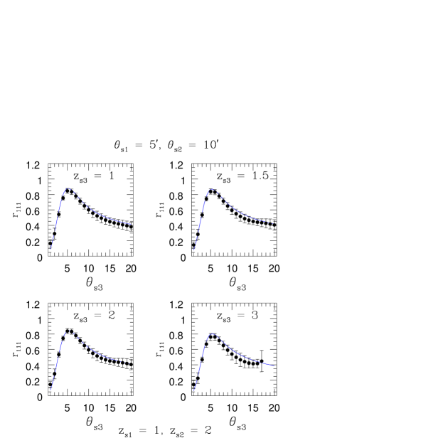
Figure 8: The three-point correlator $r_{111}$ is plotted as a function of smoothing angle $\theta_{s3}$ for the fixed pair $(\theta_{s1},\theta_{s2})=(5^{\prime},10^{\prime})$. The source redshifts are $z_{s1}=1$ and $z_{s2}=2$ while we have $z_{s3}=1$ (upper left panel), $z_{s3}=1.5$ (upper right panel), $z_{s3}=2$ (lower left panel) and $z_{s3}=3$ (lower right panel). The solid curve is the analytical model (6) while solid points with error-bars are measurements from simulation data.

We show in Fig. 7 the three-point correlation coefficient $r_{111}$ as a function of smoothing angle $\theta_{s3}$ for three fixed pairs of $(\theta_{s1},\theta_{s2})$, with equal redshifts $z_{s1}=z_{s2}=z_{s3}=1$. Of course, we recover a behaviour similar to that of Fig. 4 obtained for the SNAP survey. Moreover, we can check that the simple analytical model (6) shows a good agreement with the numerical simulations. We present in the four panels of Fig. 8 the dependence on the source redshift $z_{s3}$ of the correlator $r_{111}$, with two different redshifts $z_{s1}=1$ and $z_{s2}=2$. The dependence on $z_{s3}$ is very weak over the range $z_{s1}<z_{s3}<z_{s2}$ while $r_{111}$ decreases for larger $z_{s3}$, as expected. The agreement of the simple stellar model with numerical simulations is rather good for all cases.

4.3 Constraints on the density field

We have seen in Fig. 3 that the correlation coefficients $r_{pq}$ (or $r_{pqs}$) are almost independent of cosmological parameters. Therefore, they can be used to monitor the noise of the survey or to constrain the properties of the matter density field (e.g. the angular behaviour of the many-body correlation functions). We have checked in Figs. 5-8 that the simple stellar model (6) (which is a peculiar case of the more general class of hierarchical models) agrees rather well with numerical simulations. We now show that this agreement is not due to the independence of the correlators $r_{pqs}$ on the underlying density field. That is, although most of the dependence on cosmology has been factorized out of the ratios (9) and (10) as well as the overall amplitude of the density fluctuations (both properties are mostly probed by the one-point statistics), some information on the detailed angular behaviour of the density correlations remains in the correlation coefficients $r_{pqs}$.

To investigate this point we compare in Figs. 9-10 the predictions obtained from different analytical models. The solid line (A) is the stellar model (6) which we have used so far. Here we must note that this model is not fully defined by eq.(6) because the parameters $\tilde{S}_{p}$ vary with scale and time. More precisely, the skewness parameter $\tilde{S}_{3}$ is obtained by interpolating between the quasi-linear theory prediction and the HEPT approximation (Scoccimarro et al. 1998), see Munshi et al. (2004). Then, $\tilde{S}_{3}$ depends on the slope of the linear power-spectrum $P_{L}(k)$ and on the amplitude of the non-linear power $\Delta^{2}(k)$ at the wavenumber $k=4/({\cal D}\theta_{s})$. However, for the two-point correlations we have two angular scales $\theta_{s1},\theta_{s2}$ which can be different. Then, we extended the stellar model (6) to these cases by using:

$$\mbox{model (A):}\;\;\;\tilde{S}_{p,q}=\tilde{S}_{p+q,0}^{p/(p+q)}\tilde{S}_{0,p+q}^{q/(p+q)},$$ (13)

where we note $\tilde{S}_{p,q}$ the coefficient $\tilde{S}_{p+q}$ which appears in a cross-product of the form $\langle X_{1}^{p}X_{2}^{q}\rangle_{c}$, and the coefficient $\tilde{S}_{p+p,0}$ (resp. $\tilde{S}_{0,p+q}$) is associated with only one angular scale $\theta_{s1}$ (resp. $\theta_{s2}$) where there is no ambiguity for the typical wavenumber $k$. We have checked in sections 4.1, 4.2 that this simple model (A) agrees quite well with numerical simulations. Next, in order to evaluate the sensitivity of our predictions onto the approximation (13) we define the variant (B) by:

$$\mbox{model (B):}\;\;\;\tilde{S}_{p,q}=\min(\tilde{S}_{p+q,0};\tilde{S}_{0,p+q}).$$ (14)

Thus the two models (A) and (B) coincide for $\theta_{s1}=\theta_{s2}$ and both can be described as stellar models of the form (6). The freedom between models (A) and (B), due to the scale dependence of the parameters $\tilde{S}_{p}$, expresses the fact that the model (6) is a simple phenomenological prescription but not a fully consistent model (this would require a constant parameter $\tilde{S}_{p}$). Finally, we also define a third model (D) where many-body density correlations reduce to products of Dirac factors in real space:

$$\mbox{model (D):}\;\;\;\langle\delta({\bf x}_{1})\dots\delta({\bf x}_{p})\rangle_{c}=\delta_{D}({\bf x}_{2}-{\bf x}_{1})\dots\delta_{D}({\bf x}_{p}-{\bf x}_{1}).$$ (15)

We take the normalization coefficient in eq.(15) to be constant so that it cancels out of the correlation coefficients $r_{pq}$. For $p=2$ the model (D) merely corresponds to a white-noise power-spectrum, while for all $p\geq 2$ it corresponds to the stellar model with a white-noise power-spectrum. This model is not expected to be a good approximation of the matter density field. Its only purpose is to check whether the detailed behaviour of large-scale structures can be seen in the correlation coefficients $r_{pq}$. It gives the contribution to the coefficients $r_{pq}$ provided by sheer geometrical factors, since we have for identical source redshift distributions:

$$\mbox{model (D):}\;\;\;\langle X_{1}^{p}X_{2}^{q}\rangle_{c}\propto\int{\rm d}{\vec{\vartheta}}\;U_{1}({\vec{\vartheta}})^{p}U_{2}({\vec{\vartheta}})^{q}\;\;\;\mbox{if}\;\;\;n_{1}(z_{s})=n_{2}(z_{s}),$$ (16)

where the normalization factor which only depends on $(p+q)$ cancels out of the coefficients $r_{pq}$. The models (A), (B) and (D) extend in a straightforward manner to three-point correlators like $r_{111}$. Although the models (A), (B) and (D) yield different results despite their similarity, we can note that the predictions obtained from model (A) for the third-order correlators we study here are actually common to all models which obey $\langle\delta({\bf k}_{1})\delta({\bf k}_{2})\delta({\bf k}_{3})\rangle_{c}\propto\delta_{D}({\bf k}_{1}+{\bf k}_{2}+{\bf k}_{3})[P(k_{1})P(k_{2})F({\bf k}_{1},{\bf k}_{2})+\mbox{sym.}]$ where $F({\bf k}_{1},{\bf k}_{2})$ is any function of the angle between ${\bf k}_{1}$ and ${\bf k}_{2}$. Indeed, the angular dependence contained in $F({\bf k}_{1},{\bf k}_{2})$ is integrated out in the same manner for one-point, two-point and three-point cumulants so that it cancels out of $r_{pqs}$. Of course, the behaviour of $F({\bf k}_{1},{\bf k}_{2})$ would show up if we consider different smoothing cells which are not centered on the same line-of-sight.

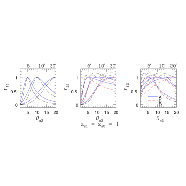
Figure 9: The two-point correlation coefficients $r_{pq}$ as in Fig. 5, for $\theta_{s1}=5^{\prime},10^{\prime}$ and $20^{\prime}$ and $z_{s1}=z_{s2}=1$. The different line-styles represent different analytical models: the basic stellar model (A), the variant (B) (see main text) and the Dirac-product model (D).

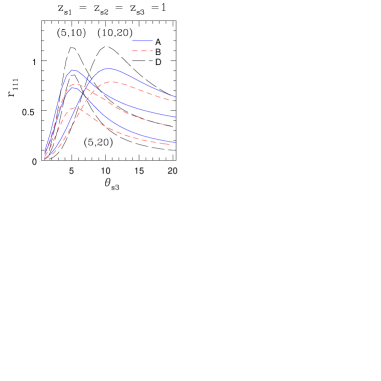
Figure 10: The three-point correlation coefficient $r_{111}$ as in Fig. 7, at $z_{s1}=z_{s2}=z_{s3}=1$ for three pairs of smoothing angles $(\theta_{s1},\theta_{s2})$. The different line-styles represent different analytical models: the basic stellar model (A), the variant (B) (see main text) and the Dirac-product model (D).

We show in Figs. 9-10 these three models (A) (solid line), (B) (dashed line) and (D) (dot-dashed line). We can see that the differences are quite apparent and are larger than the error-bars obtained from numerical simulations in Figs. 5-8. Therefore, although the correlation coefficients $r_{pq}$ and $r_{pqs}$ are almost insensitive to cosmology they show a significant dependence on the properties of the many-body density correlations (note that models (A) and (B) are quite close). This separation between the background cosmology (which can be probed by one-point statistics) and the large-scale structures themselves should be quite useful to discriminate between both classes of phenomena and to probe gravitational clustering. In particular, we can note that the differences between various models seen in Figs. 9-10 are sufficiently large to be detected by future surveys like SNAP, see the error-bars in Figs. 1-4. Finally, it appears that the simple stellar model (A) defined from eqs.(6),(13) works best and provides a good description of the actual density field for these purposes, as checked in sections  4.1, 4.2.

5 Discussion

We have extended the formalism developed in Munshi & Coles (2002) to study the cross-correlations among various angular scales covering a range of redshift bins. We define the correlation coefficients $r_{pqs}$ in such a way as to minimize the dependence on cosmological parameters and on the redshift distribution of the sources. Since the aperture-mass window is very narrow in Fourier space they provide a useful tool to study gravitational clustering, through both the power spectrum and the bi-spectrum. In particular, higher order coefficients $r_{pqs}$ where $p+q+s>2$ carry useful information about the level of non-Gaussianity in the projected density field. Generalizing our previous studies from two-point statistics to three-point statistics we have used $r_{111}$ as a diagnostics of the bi-spectrum. Indeed, although one-point or two-point cumulants or correlators such as $r_{21}$ also contain useful information about the bi-spectrum, $r_{111}$ allows one to probe the bi-spectrum in more details. These tools can be used not only to probe gravitational instability scenarios but also to put constraints on primordial non-Gaussianities or higher-dimensional theories of gravitation. We plan to study such issues in more detail in future works. On the other hand, these estimators can also be used to monitor hidden systematics.

We have presented a detailed analysis of these correlation coefficients for the wide SNAP survey, as an illustration for future weak-lensing surveys. We have computed both the expected signal and its error-bars, taking into account the intrinsic ellipticity of galaxies and the cosmic variance. The cumulant estimators $H_{pqs}$ are built from the moment estimators $M_{pqs}$ so as to lower their scatter. Note that we take into account the non-Gaussianities of the density field in the computation of the error-bars. The scatter associated with SNAP class experiments is extremely small for second-order statistics such as the variance or the correlation $r_{11}$ but it increases very fast with the order of the statistics. Nevertheless, these surveys are still able to probe third-order statistics with a reasonable accuracy. This should allow one to get meaningful constraints on large-scale structures or on the observational noise.

Next, we have compared a simple stellar model with the results obtained from numerical simulations. We had shown in previous papers that this simple analytical model agrees reasonably well with simulations for one-point cumulants (e.g., Munshi et al. 2004). We have found in this work that it also gives good predictions for two-point and three-point statistics over the entire range of redshifts and smoothing scales of interest. Therefore, this simple model provides a useful tool to investigate in great details weak-lensing effects measured through smoothed statistics like the aperture-mass.

Finally, we have checked that the agreement between this simple model and numerical simulations is not due to a weak sensitivity of these correlators onto the structure of the underlying density field. Indeed, introducing two other models for the detailed behaviour of the matter density correlations we have found that the correlation coefficients $r_{pqs}$ show a significant dependence on the properties of large-scale structures, which can be detected in future surveys like SNAP. Therefore, such observations can yield constraints on the structure of the matter density field. Note however that at order three the predictions obtained from the simple stellar model (6) are shared by a wider class of models (e.g. all usual hierarchical models). In order to discriminate these various models one would need to go up to fourth-order statistics (where one can draw several hierarchical diagrams for instance) but error-bars become too large to give good constraints.

In this paper we have only considered the cases where the smoothing patches are all lined up along the same radial direction, although they can have different redshift distributions or smoothing radii. It is trivial to generalise our results to cases where various patches are separated by a given separation angle. However with increasing separation the signal to noise will degrade which may prevent practical applications. We have only used the compensated filter associated with the aperture-mass which can directly be constructed from shear maps. Its presents the advantages of probing a narrow range of wavenumbers and of giving a non-zero signal for third-order statistics. Nevertheless our formalism is completely general and we can replace this compensated filter by any window (like a top-hat for the convergence or a modified top-hat with angular dependence for shear components). However, in such cases the number of patches which can carry completely independent information will decrease (because of the contribution of long wavelengths) which will increase observational error-bars.

Appendix A 3pt Correlators

As in Munshi & Valageas (2004), the three-point cumulants $\langle M_{\rm ap1}^{p}M_{\rm ap2}^{q}M_{\rm ap3}^{s}\rangle_{c}$ can be estimated from the estimators $M_{pqs}$ defined by:

$$M_{pqs}=\frac{(\pi\theta_{s1}^{2})^{p}(\pi\theta_{s2}^{2})^{q}(\pi\theta_{s3}^{2})^{s}}{(N_{1})_{p}(N_{2})_{q}(N_{3})_{s}}\sum_{\{(i_{1},\dots,i_{p});(j_{1},\dots,j_{p});(l_{1},\dots,l_{p})\}}^{\{N_{1};N_{2};N_{3}\}}Q_{i_{1}}\epsilon_{{\rm t}i_{1}}\dots Q_{i_{p}}\epsilon_{{\rm t}i_{p}}\;\;Q_{j_{1}}\epsilon_{{\rm t}j_{1}}\dots Q_{j_{q}}\epsilon_{{\rm t}j_{q}}\;\;Q_{l_{1}}\epsilon_{{\rm t}l_{1}}\dots Q_{l_{s}}\epsilon_{{\rm t}l_{s}}.$$ (17)

Here, $N_{1}$, $N_{2}$ and $N_{3}$ are the number of galaxies within the patches $\pi\theta_{s1}^{2}$, $\pi\theta_{s2}^{2}$ and $\pi\theta_{s3}^{2}$ for the surveys $(1,2,3)$, while $N_{ij}$ and $N_{123}$ are the number of common galaxies to two or all three samples, and we noted $(N)_{p}=N(N-1)..(N-p+1)=N!/(N-p)!$. In eq.(17) we only sum over combinations of distinct galaxies and we assumed that $N_{j}\gg 1$. Thus, for $M_{111}$ we sum over $N_{1}N_{2}N_{3}-N_{12}N_{3}-N_{13}N_{2}-N_{23}N_{1}+2N_{123}\simeq N_{1}N_{2}N_{3}$ terms. We note $Q_{j}=Q_{M_{\rm ap}}({\vec{\vartheta}}_{j})$ the value of the filter $Q_{M_{\rm ap}}({\vec{\vartheta}})$ at the location ${\vec{\vartheta}}_{j}$ of the galaxy $j$ and $\epsilon_{{\rm t}j}$ its tangential ellipticity. The filter $Q_{M_{\rm ap}}$ is given by:

$$Q_{M_{\rm ap}}({\vec{\vartheta}})=\frac{\Theta(\vartheta<\theta_{s})}{\pi\theta_{s}^{2}}\;6\;\left(\frac{\vartheta}{\theta_{s}}\right)^{2}\left(1-\frac{\vartheta^{2}}{\theta_{s}^{2}}\right).$$ (18)

The mean and the dispersion $\sigma$ of $M_{pqs}$ are:

$$\langle M_{pqs}\rangle=\langle M_{\rm ap1}^{p}M_{\rm ap2}^{q}M_{\rm ap3}^{s}\rangle,\;\;\;\sigma^{2}(M_{pqs})=\langle M_{pqs}^{2}\rangle-\langle M_{pqs}\rangle^{2}.$$ (19)

The scatter $\sigma(M_{pqs})$ only involves the variance $\sigma_{*}^{2}=\langle|\epsilon_{*}|^{2}\rangle$ of the galaxy intrinsic ellipticities (even if the latter are not Gaussian). The latter enters the dispersion $\sigma^{2}$ through the combinations $\rho_{j}$ and $\rho_{ij}$ defined by:

$$\rho_{j}=\frac{5N_{j}\langle M_{{\rm ap}j}^{2}\rangle_{c}}{3\sigma_{*}^{2}}\;\;\;\mbox{and}\;\;\;\rho_{ij}=\frac{5N_{i}N_{j}\langle M_{{\rm ap}i}M_{{\rm ap}j}\rangle_{c}}{N_{ij}3\sigma_{*}^{2}}.$$ (20)

The quantity $\rho_{j}$ is the signal-to-noise ratio of the weak-lensing variance over the random intrinsic ellipticity. It also measures the relative importance of the cosmic variance as compared with the galaxy intrinsic ellipticities to the scatter of relevant estimators (intrinsic ellipticities can be neglected if $\rho\gg 1$).

The estimators $M_{pqs}$ defined in eq.(17) correspond to a single direction onto the sky, around which are centered the three smoothing windows of radii $\theta_{sj}$. In practice, we can average over $N_{c}$ such directions on the sky with no overlap. This yields the estimators ${\cal M}_{pqs}$ defined by:

$${\cal M}_{pqs}=\frac{1}{N_{c}}\sum_{n=1}^{N_{c}}M_{pqs}^{(n)},\;\;\;\mbox{whence}\;\;\;\langle{\cal M}_{pqs}\rangle=\langle M_{pqs}\rangle=\langle M_{\rm ap1}^{p}M_{\rm ap2}^{q}M_{\rm ap3}^{s}\rangle\;\;\;\mbox{and}\;\;\;\sigma({\cal M}_{pqs})=\frac{\sigma(M_{pqs})}{\sqrt{N_{c}}},$$ (21)

where $M_{pqs}^{(n)}$ is the estimator $M_{pqs}$ for the cell $n$ and we assumed that these cells are sufficiently well separated so as to be uncorrelated. The estimators $M_{pqs}$ and ${\cal M}_{pqs}$ provide a measure of the moments of weak lensing observables. However, as shown in Valageas et al. (2004b), it is better to first consider cumulant-inspired estimators $H_{pqs}$ and ${\cal H}_{pqs}$. For the case of the quantity $\langle M_{\rm ap1}M_{\rm ap2}M_{\rm ap3}\rangle_{c}$ the relevant estimator $H_{111}$ is:

$$H_{111}=M_{111}-{\cal M}_{011}M_{100}-{\cal M}_{101}M_{010}-{\cal M}_{110}M_{001},\;\;\;{\cal H}_{111}=\frac{1}{N_{c}}\sum_{n=1}^{N_{c}}H_{111}^{(n)},\;\;\;\mbox{whence}\;\;\;\langle{\cal H}_{111}\rangle=\langle M_{\rm ap1}M_{\rm ap2}M_{\rm ap3}\rangle_{c}.$$ (22)

Then the dispersion $\sigma^{2}(H_{111})$ reads:

$$\sigma^{2}(H_{111})=\langle M_{\rm ap1}^{2}M_{\rm ap2}^{2}M_{\rm ap3}^{2}\rangle_{c}+\langle M_{\rm ap2}^{2}M_{\rm ap3}^{2}\rangle_{c}\langle M_{\rm ap1}^{2}\rangle_{c}\left[1+{1\over\rho_{1}}\right]+\langle M_{\rm ap1}^{2}M_{\rm ap3}^{2}\rangle_{c}\langle M_{\rm ap2}^{2}\rangle_{c}\left[1+{1\over\rho_{2}}\right]$$ (23)

$$+\langle M_{\rm ap1}^{2}M_{\rm ap2}^{2}\rangle_{c}\langle M_{\rm ap3}^{2}\rangle_{c}\left[1+{1\over\rho_{3}}\right]+\langle M_{\rm ap1}^{2}M_{\rm ap2}M_{\rm ap3}\rangle_{c}\langle M_{\rm ap2}M_{\rm ap3}\rangle_{c}2\left[1+{1\over\rho_{23}}\right]+\langle M_{\rm ap1}M_{\rm ap2}^{2}M_{\rm ap3}\rangle_{c}\langle M_{\rm ap1}M_{\rm ap3}\rangle_{c}2\left[1+{1\over\rho_{13}}\right]$$

$$+\langle M_{\rm ap1}M_{\rm ap2}M_{\rm ap3}^{2}\rangle_{c}\langle M_{\rm ap1}M_{\rm ap2}\rangle_{c}2\left[1+{1\over\rho_{12}}\right]+2\langle M_{\rm ap1}M_{\rm ap2}^{2}\rangle_{c}\langle M_{\rm ap1}M_{\rm ap3}^{2}\rangle_{c}+2\langle M_{\rm ap1}^{2}M_{\rm ap2}\rangle_{c}\langle M_{\rm ap2}M_{\rm ap3}^{2}\rangle_{c}$$

$$+2\langle M_{\rm ap1}^{2}M_{\rm ap3}\rangle_{c}\langle M_{\rm ap2}^{2}M_{\rm ap3}\rangle_{c}+3\langle M_{\rm ap1}M_{\rm ap2}M_{\rm ap3}\rangle_{c}^{2}+\langle M_{\rm ap1}^{2}\rangle_{c}\langle M_{\rm ap2}^{2}\rangle_{c}\langle M_{\rm ap3}^{2}\rangle_{c}\left[1+{1\over\rho_{1}}\right]\left[1+{1\over\rho_{2}}\right]\left[1+{1\over\rho_{3}}\right]$$

$$+\langle M_{\rm ap1}^{2}\rangle_{c}\langle M_{\rm ap2}M_{\rm ap3}\rangle_{c}^{2}\left[1+{1\over\rho_{1}}\right]\left[1+{1\over\rho_{23}}\right]^{2}+\langle M_{\rm ap2}^{2}\rangle_{c}\langle M_{\rm ap1}M_{\rm ap3}\rangle_{c}^{2}\left[1+{1\over\rho_{2}}\right]\left[1+{1\over\rho_{13}}\right]^{2}$$

$$+\langle M_{\rm ap3}^{2}\rangle_{c}\langle M_{\rm ap1}M_{\rm ap2}\rangle_{c}^{2}\left[1+{1\over\rho_{3}}\right]\left[1+{1\over\rho_{12}}\right]^{2}+\langle M_{\rm ap1}M_{\rm ap2}\rangle_{c}\langle M_{\rm ap1}M_{\rm ap3}\rangle_{c}\langle M_{\rm ap2}M_{\rm ap3}\rangle_{c}2\left[1+{1\over\rho_{12}}\right]\left[1+{1\over\rho_{13}}\right]\left[1+{1\over\rho_{23}}\right]$$

while the scatter of the estimator $M_{111}$ can be obtained from:

$$\sigma^{2}(M_{111}) = \sigma^{2}(H_{111})+2\langle M_{\rm ap1}^{2}M_{\rm ap2}M_{\rm ap3}\rangle_{c}\langle M_{\rm ap2}M_{\rm ap3}\rangle_{c}+2\langle M_{\rm ap1}M_{\rm ap2}^{2}M_{\rm ap3}\rangle_{c}\langle M_{\rm ap1}M_{\rm ap3}\rangle_{c}$$ (24)

$$+2\langle M_{\rm ap1}M_{\rm ap2}M_{\rm ap3}^{2}\rangle_{c}\langle M_{\rm ap1}M_{\rm ap2}\rangle_{c}+\langle M_{\rm ap1}^{2}\rangle_{c}\langle M_{\rm ap2}M_{\rm ap3}\rangle_{c}^{2}\left[1+{1\over\rho_{1}}\right]+\langle M_{\rm ap2}^{2}\rangle_{c}\langle M_{\rm ap1}M_{\rm ap3}\rangle_{c}^{2}\left[1+{1\over\rho_{2}}\right]$$

$$+\langle M_{\rm ap3}^{2}\rangle_{c}\langle M_{\rm ap1}M_{\rm ap2}\rangle_{c}^{2}\left[1+{1\over\rho_{3}}\right]+\langle M_{\rm ap1}M_{\rm ap2}\rangle_{c}\langle M_{\rm ap1}M_{\rm ap3}\rangle_{c}\langle M_{\rm ap2}M_{\rm ap3}\rangle_{c}\left[6+{2\over\rho_{12}}+{2\over\rho_{13}}+{2\over\rho_{23}}\right].$$

In order to obtain the dispersion of the correlation coefficient $r_{111}$ we also need the scatter of the cross-product $\sigma^{2}(H_{111};H_{300})=\langle H_{111}H_{300}\rangle-\langle H_{111}\rangle\langle H_{300}\rangle$ which reads:

$$\sigma^{2}(H_{111};H_{300}) = \langle M_{\rm ap1}^{4}M_{\rm ap2}M_{\rm ap3}\rangle_{c}+\langle M_{\rm ap1}^{3}M_{\rm ap2}\rangle_{c}\langle M_{\rm ap1}M_{\rm ap3}\rangle_{c}3\left[1+{1\over\rho_{13}}\right]+\langle M_{\rm ap1}^{3}M_{\rm ap3}\rangle_{c}\langle M_{\rm ap1}M_{\rm ap2}\rangle_{c}3\left[1+{1\over\rho_{12}}\right]$$ (25)

$$+\langle M_{\rm ap1}^{2}M_{\rm ap2}M_{\rm ap3}\rangle_{c}\langle M_{\rm ap1}^{2}\rangle_{c}3\left[1+{1\over\rho_{1}}\right]+3\langle M_{\rm ap1}^{3}\rangle_{c}\langle M_{\rm ap1}M_{\rm ap2}M_{\rm ap3}\rangle_{c}+6\langle M_{\rm ap1}^{2}M_{\rm ap2}\rangle_{c}\langle M_{\rm ap1}^{2}M_{\rm ap3}\rangle_{c}$$

$$+\langle M_{\rm ap1}^{2}\rangle_{c}\langle M_{\rm ap1}M_{\rm ap2}\rangle_{c}\langle M_{\rm ap1}M_{\rm ap3}\rangle_{c}6\left[1+{1\over\rho_{1}}\right]\left[1+{1\over\rho_{12}}\right]\left[1+{1\over\rho_{13}}\right],$$

while $\sigma^{2}(M_{111};M_{300})$ writes:

$$\sigma^{2}(M_{111};M_{300}) = \sigma^{2}(H_{111};H_{300})+\langle M_{\rm ap1}^{4}\rangle_{c}\langle M_{\rm ap2}M_{\rm ap3}\rangle_{c}+\langle M_{\rm ap1}^{3}M_{\rm ap2}\rangle_{c}\langle M_{\rm ap1}M_{\rm ap3}\rangle_{c}+\langle M_{\rm ap1}^{3}M_{\rm ap3}\rangle_{c}\langle M_{\rm ap1}M_{\rm ap2}\rangle_{c}$$ (26)

$$+3\langle M_{\rm ap1}^{2}M_{\rm ap2}M_{\rm ap3}\rangle_{c}\langle M_{\rm ap1}^{2}\rangle_{c}+\langle M_{\rm ap1}^{2}\rangle_{c}^{2}\langle M_{\rm ap2}M_{\rm ap3}\rangle_{c}3\left[1+{1\over\rho_{1}}\right]$$

$$+\langle M_{\rm ap1}^{2}\rangle_{c}\langle M_{\rm ap1}M_{\rm ap2}\rangle_{c}\langle M_{\rm ap1}M_{\rm ap3}\rangle_{c}\left[6+{3\over\rho_{12}}+{3\over\rho_{13}}\right].$$

We can check that as for one-point and two-point cumulants, the estimators $H_{pqs}$ have a lower scatter than their counterparts $M_{pqs}$ and their dispersion only depends on the combination $(1+1/\rho)$.

Finally, the three-point correlation coefficient $r_{111}$ can be estimated from the estimator ${\cal R}_{111}$:

$${\cal R}_{111}=\frac{{\cal H}_{111}}{{\cal H}_{300}^{1/3}{\cal H}_{030}^{1/3}{\cal H}_{003}^{1/3}}\;\;\;\mbox{with}\;\;\;\langle{\cal R}_{111}\rangle\simeq r_{111}$$ (27)

and:

$$\sigma^{2}({\cal R}_{111}) \simeq r_{111}^{2}\Biggl{\{}\frac{\sigma^{2}({\cal H}_{111})}{\langle{\cal H}_{111}\rangle^{2}}+\frac{1}{9}\frac{\sigma^{2}({\cal H}_{300})}{\langle{\cal H}_{300}\rangle^{2}}+\frac{1}{9}\frac{\sigma^{2}({\cal H}_{030})}{\langle{\cal H}_{030}\rangle^{2}}+\frac{1}{9}\frac{\sigma^{2}({\cal H}_{003})}{\langle{\cal H}_{003}\rangle^{2}}-\frac{2}{3}\frac{\sigma^{2}({\cal H}_{111};{\cal H}_{300})}{\langle{\cal H}_{111}\rangle\langle{\cal H}_{300}\rangle}-\frac{2}{3}\frac{\sigma^{2}({\cal H}_{111};{\cal H}_{030})}{\langle{\cal H}_{111}\rangle\langle{\cal H}_{030}\rangle}$$ (28)

$$-\frac{2}{3}\frac{\sigma^{2}({\cal H}_{111};{\cal H}_{003})}{\langle{\cal H}_{111}\rangle\langle{\cal H}_{003}\rangle}+\frac{2}{9}\frac{\sigma^{2}({\cal H}_{300};{\cal H}_{030})}{\langle{\cal H}_{300}\rangle\langle{\cal H}_{030}\rangle}+\frac{2}{9}\frac{\sigma^{2}({\cal H}_{300};{\cal H}_{003})}{\langle{\cal H}_{300}\rangle\langle{\cal H}_{003}\rangle}+\frac{2}{9}\frac{\sigma^{2}({\cal H}_{030};{\cal H}_{003})}{\langle{\cal H}_{030}\rangle\langle{\cal H}_{003}\rangle}\Biggl{\}}.$$

Here we assumed that the scatter of ${\cal R}_{111}$ is small and can be linearized. The various terms in eq.(28) can be obtained from the expressions derived above or from Munshi & Valageas (2004).

References

- [1] Bacon D.J., Refregier A., Ellis R.S., 2000, MNRAS, 318, 625
- [2] Barber A. J., Munshi D., Valageas P., 2004, MNRAS, 347, 665
- [3] Bernardeau F., Schaeffer R., 1992, A&A, 255, 1
- [4] Bernardeau F., Valageas P., 2000, A&A, 364, 1
- [5] Couchman H. M. P., Barber A. J., Thomas P. A., 1999, MNRAS, 308, 180
- [6] Bernardeau F., Valageas P., 2000, A&A, 364, 1
- [7] Bernardeau F., Colombi S., Gaztanaga E., Scoccimarro R., Phys.Rept., (2002), 367, 1
- [8] Couchman H. M. P., Thomas P. A., Pearce F. R., 1995, ApJ., 452,
- [9] Fry J.N., 1984, ApJ, 279, 499
- [10] Hoekstra H., Yee H. K. C., Gladders M. D., 2002, ApJ, 577, 595
- [11] Jain B., Seljak U., 1997, ApJ, 484, 560
- [12] Jain B., Seljak U., White S.D.M., 2000, ApJ, 530, 547
- [13] Jaroszyn’ski M., Park C., Paczynski B., Gott J.R., 1990, ApJ, 365, 22
- [14] Kaiser N., 1998, ApJ, 498, 26
- [15] Munshi D., Coles P., Melott A.L., 1999a, MNRAS, 307, 387
- [16] Munshi D., Coles P., Melott A.L., 1999b, MNRAS, 310, 892
- [17] Munshi D., Melott A.L., Coles P., 1999, MNRAS, 311, 149
- [18] Munshi D., Coles P., 2003, MNRAS, 338, 846
- [19] Munshi D., Jain B., 2000, MNRAS, 318, 109
- [20] Munshi D., Jain B., 2001, MNRAS, 322, 107
- [21] Munshi D., Valageas P. & Barber A., 2004, MNRAS, in press
- [22] Munshi D., Valageas P. 2004, MNRAS, in press
- [23] Peacock J.A., Dodds S.J., 1996, MNRAS, 280, L19
- [24] Peacock J. A., Smith R. E., 2000, MNRAS, 318, 1144
- [25] Schneider P., Weiss A., 1988, ApJ, 330,1
- [26] Schneider P., Van Waerbeke L., Jain B., Kruse G., 1998,
- [27] Stebbins A., 1996, astro-ph/9609149
- [28] Szapudi I., Szalay A.S., 1993, ApJ, 408, 43
- [29] Szapudi I., Szalay A.S., 1997, ApJ, 481, L1
- [30] Takada M., Jain B., 2003, MNRAS, 344, 857
- [31] Valageas P., 2000a, A&A, 354, 767
- [32] Valageas P., 2000b, A&A, 356, 771
- [33] Valageas P., Barber A. J., Munshi D., 2003, MNRAS (in press) (astro-ph/0303472)
- [34] Van Waerbeke L., Bernardeau F., Mellier Y., 1999, A& A, 342, 15
- [35] Van Waerbeke L., Mellier Y., Pelló R., Pen U.-L., McCracken H. J., Jain B., 2002, A&A, 393, 369
- [36] Villumsen J.V., 1996, MNRAS, 281, 369
- [37] Wambsganss J., Cen R., Ostriker J.P., 1998, ApJ, 494, 298
- [38] Wambsganss J., Cen R., Xu G., Ostriker J.P., 1997, ApJ, 494, 29