A Time-Dependent Radiative Model of HD209458b

We present a time-dependent radiative model of the atmosphere of HD209458b and investigate its thermal structure and chemical composition. In a first step, the stellar heating profile and radiative timescales were calculated under planet-averaged insolation conditions. We find that 99.99% of the incoming stellar flux has been absorbed before reaching the 7 bar level. Stellar photons cannot therefore penetrate deeply enough to explain the large radius of the planet. We derive a radiative time constant which increases with depth and reaches about 8 hr at 0.1 bar and 2.3 days at 1 bar. Time-dependent temperature profiles were also calculated, in the limit of a zonal wind that is independent on height (i.e. solid-body rotation) and constant absorption coefficients. We predict day-night variations of the effective temperature of $\sim$600 K, for an equatorial rotation rate of 1 km s^-1, in good agreement with the predictions by Showman & Guillot (2002). This rotation rate yields day-to-night temperature variations in excess of 600 K above the 0.1-bar level. These variations rapidly decrease with depth below the 1-bar level and become negligible below the $\sim$5–bar level for rotation rates of at least 0.5 km s^-1. At high altitudes (mbar pressures or less), the night temperatures are low enough to allow sodium to condense into Na₂S. Synthetic transit spectra of the visible Na doublet show a much weaker sodium absorption on the morning limb than on the evening limb. The calculated dimming of the sodium feature during planetary transites agrees with the value reported by Charbonneau et al. (2002).

1 Introduction

The discovery of HD209458b (Charbonneau et al. (2000); Henry et al. (2000)) allows for the first time probing directly the structure of a planet outside our Solar System. Indeed, the fact that it transits in front of its star allows both the measurement of its radius and the spectroscopic observation of its atmosphere.

Quantitatively, HD209458 is a G0 subgiant, with a mass $M_{\star}=1.06M_{\odot}$, radius $R_{\star}=1.18R_{\odot}$ and age $t_{\star}=5.2$ Gyr, with uncertainties of 10% or more (Cody & Sasselov 2002). The planet orbits the star in 3.524739 days (Robichon & Arenou 2000), at a distance $\sim 0.045$ AU. Models of the star imply that its radius is $R$ = 92 200–109 000 km (about 40% more than Jupiter) for a mass $M=0.69\pm 0.02\,M_{\rm J}$ (Brown et al. 2001; Cody & Sasselov 2002).

The relatively large radius of the planet appears difficult to explain using standard evolution models (Bodenheimer et al. 2001, 2003; Guillot & Showman 2002; Baraffe et al. 2003). Guillot & Showman (2002) concluded that, for a realistic model of the outer atmosphere irradiated by the parent star, an extra energy source is needed at deep levels to explain HD209458’s radius. It could result from the penetration of a small fraction of the stellar flux at pressures of tens of bars or from kinetic energy produced from the stellar heating and transported downwards to the interior region. The same conclusion was reached by Baraffe et al. (2003) from model calculations directly coupling the irradiated outer atmosphere and the interior. However, the possibility that systematic errors both in the determination of the stellar radius and atmospheric properties of the planet remains (Burrows et al. 2003).

In order to accurately model the evolution of extrasolar giant planets, and hence gain information on their composition, one has to understand how their atmospheres intercept and reemit the stellar irradiation. The problem is especially accute for planets like 51 Peg b and HD209458b (hereafter Pegasides) which are believed to be locked into synchronous rotation (Guillot et al. 1996) due to their proximity to their star. As a consequence the amount of irradiation received on the day side and the insolation pattern are unlike what is experienced by any planet in the Solar System.

Several studies have investigated the radiative equilibrium structure of Pegasides, treating the atmosphere as a one–dimensional column receiving an average flux from above and a smaller intrinsic flux from below. In these models, the stellar heat is either evenly distributed over the entire planet (Seager & Sasselov 1998, 2000; Goukenleuque et al. 2000), or redistributed only over the day side (Sudarsky et al. 2003; Baraffe et al. 2003; Burrows et al. 2003), or even not redistributed at all (Barman et al. 2001; Burrows et al. 2003). In fact, in a planetary atmosphere, winds carry part of the stellar heat from the day side to the night side and from equator to poles, so that the thermal structure depends not only on the insolation pattern but also on the dynamics.

Two recent dynamical studies (Showman & Guillot 2002; Cho et al. 2003) have shown that the atmospheric structure probably presents strong latitudinal and longitudinal variations in temperature (and hence composition). These two investigations differ in several respects: Showman & Guillot (2002) used analytical arguments to show that the atmospheres of Pegasides should have strong winds ($\sim 1\rm\,km\,s^{-1}$) and relatively strong day-night and equator-to-pole temperature contrasts ($\sim 500\,$K near optical depth unity). These estimates are confirmed by preliminary 3D simulations done using the EPIC (Explicit Planetary Isentropic Coordinate) model with a radiative time constant of 2.3 days. These simulations tend to yield a prograde equatorial jet and thus imply that the atmosphere could superrotate as a whole (as is the case for Venus). On the other hand, Cho et al. (2003) solved 2D shallow-water equations, assuming a characteristic wind speed, related to the mean kinetic energy, of 50 to 1000 m s^-1 and a radiative equilibrium time of 10 days. Their simulations yield a circulation which is characterized by moving polar vortexes around the poles and $\sim$ 3 broad zonal jets. For the highest speed considered (1 km s^-1), the temperature minimum is about 800 K and the maximum temperature contrast is $\sim 1000$ K.

The goal of the present study is to apply a time-dependent radiative transfer model to the case of HD209458b in order to: (i) determine its mean temperature structure and stellar heating profile; (ii) estimate the characteristic radiative heating/cooling timescale as a function of depth; (iii) model longitudinal temperature variations assuming a solid rotation; (iv) infer consequences for the variations in chemical composition in light of the spectroscopic transit observations.

In Section 2, we present our time-dependent radiative transfer model. We then apply the model to HD209458b. In Section 3 we compare models obtained for averaged insolation conditions, and calculate the corresponding radiative timescales. In Section 4, we calculate the longitude-dependent thermal structure of the atmosphere by assuming a solid body rotation, mimicking a uniform zonal wind. The variations in the chemical composition induced by temperature variations are investigated with the emphasis on the condensation of sodium. A summary of the results and a conclusion are presented in Section 5.

2 The Atmospheric Model

2.1 Physical problem

In a one-dimensional model, the evolution of the temperature profile in an atmosphere under hydrostatic equilibrium is related to the net flux $F$ by the following energy equation:

$$\frac{dT}{dt}=\frac{mg}{C_{\rm p}}\left(\frac{dF}{dp}\right)\quad{\rm,}$$ (1)

where $mg$ is the mean molecular weight and $C_{\rm p}$ is the mean specific heat. The net flux is divided into the thermal flux emitted by the atmosphere $F_{\rm IR}$ (upward - downward) and the net stellar flux $F_{\star}$ (downward - upward), so that $F=F_{\rm IR}-F_{\star}$. Equation 1 can then be rewritten as:

$$\frac{dT}{dt}=\left(h(p)-c(p)\right)\quad{\rm,}$$ (2)

where $h(p)=-\frac{mg}{C_{\rm p}}\frac{dF_{\star}}{dp}$ is the heating rate and $c(p)=-\frac{mg}{C_{\rm p}}\frac{dF_{\rm IR}}{dp}$ is the cooling rate.

Radiative equilibrum corresponds to a steady-state solution of the energy equation and is thus obtained by setting the left-hand term of Eqs. 1–2 to zero. In this case, the flux is conservative and heating and cooling rates are equal at any level in the atmosphere. In a first step, we calculate the radiative equilibrium solution for HD209458b, using a planetary-averaged stellar irradiation. In a second step, we investigate the variations in the temperature profile due to the time-varying insolation, which requires solving Eq. 2.

2.2 Numerical method

We use the atmosphere code described in Goukenleuque et al. (2000), with, in the present model, an atmospheric grid of $N=96$ levels from $3\times 10^{3}$ to $1\times 10^{-6}$ bar. To calculate $F_{\star}$ as a function of pressure level $p$, we solve the radiative equation of transfer with scattering in the two-stream approximation and in plane-parallel geometry using a monochromatic line-by-line code. The boundary condition is that the incident downward flux $F_{\star}^{\downarrow}(0)$ is given by:

$$F_{\star}^{\downarrow}(0)=\alpha\pi\left(\frac{R_{\star}}{a}\right)^{2}B_{\nu}(T_{\star})\quad{\rm,}$$ (3)

where $R_{\star}$ is the star’s radius, $a$ the distance of the planet to the star’s surface, and $B_{\nu}(T_{\star})$ is the monochromatic Planck function at the star’s brightness temperature $T_{\star}$. To solve for steady-state radiative equilibrium, we consider disk-averaged insolation conditions, and thus use $\alpha=\frac{1}{4}$. For our time-dependent calculations, we use $\alpha$ = $\pi$ max[$\cos(\lambda)$,0], where $\lambda$ is the zenith angle of the star. The stellar flux is calculated from 0.3 to 6 $\mu$m (1700-32000 cm^-1). It is assumed that shortward of 0.3 $\mu$m photons are either scattered conservatively or absorbed above the atmospheric grid ($p<1$ $\mu$bar) and thus do not participate to the energy budget.

The planetary thermal flux is calculated from 0.7 to 9 $\mu$m. At level $p_{\rm i}$, it can be expressed as:

$$F_{\rm IR}=\sum_{k}\sum_{j=1}^{N}a_{\rm i,j,k}B_{\rm k}\left(T_{\rm j}\right)\quad{\rm,}$$ (4)

where $B_{\rm k}\left(T_{\rm j}\right)$ is the Planck function at the temperature $T_{\rm j}$ of pressure level $p_{\rm j}$ and at frequency $\nu_{\rm k}$, and $a_{\rm i,j,k}$ (= $a_{\rm j,i,k}$) is a coupling term related to the transmittance between levels $p_{\rm i}$ and $p_{\rm j}$, averaged over a frequency interval centered at $\nu_{\rm k}$ (Goukenleuque et al. 2000). We use an interval width of 20 cm^-1. These coefficients are calculated through a line-by-line radiative transfer code with no scattering. Below the lower boundary located at level $p_{1}$, an isothermal layer of infinite optical depth is assumed with a temperature $T_{\rm gr}$. It does not represent the actual temperature profile in the interior. In fact, for numerical reasons, what is exactly set in the model is the upward flux at the lower boundary.

2.2.1 Steady-state case

Starting from an initial guess temperature profile and the associated abundance gas profiles, stellar and thermal fluxes are computed on the atmospheric grid. The heating and cooling rates, $h(p_{\rm i})$ and $c(p_{\rm i})$, defined above are then calculated. At each level of the grid, the temperature is modified by an amount:

$$\Delta T_{\rm i}=\epsilon(p_{\rm i})\left[h(p_{\rm i})-c(p_{\rm i})\right]+\eta(p_{\rm i})\left(T_{\rm i-1}-2T_{\rm i}+T_{\rm i+1}\right)$$ (5)

The coefficient $\epsilon(p)$, analogous to a time step, increases with pressure to account for the increase of the radiative time constant with depth and thus to speed up convergence. Its value is about one hour in the upper layers and is as long as few days in the deepest layers.

The second term in the equation introduces some numerical dissipation needed to avoid instabilities at high pressure levels where the atmospheric layers are optically thick. The coefficient $\eta(p)$ is set to $1\times 10^{-3}$ above the 0.3–bar pressure level and reaches 2% at the lower boundary ($p_{1}$). The temperature $T_{gr}$ beneath pressure level $p_{1}$ is set to $T_{1}+\delta T_{1}$, where $\delta T_{1}$ is calculated to yield $F_{\rm IR}(p_{1})=F_{\rm int}$. The thermal flux is then calculated using the updated temperature profile and the procedure is iterated until the condition $h(p_{i})=c(p_{i})$ is fulfilled at each level with a precision of 5%.

A convective adjustment is then applied to the solution profile in regions where the radiative gradient exceeds the adiabatic value. In these convective regions, the gradient is set to the adiabatic value and the energy flux then includes both convective and radiative components ( Eq. 1 does not hold anymore).

After convergence, the equilibrium gas profiles are re-calculated using the solution temperature profile. The stellar flux deposition and the $a_{\rm i,j,k}$ coefficients involved in the calculation of the thermal flux are then re-computed and a new temperature profile is obtained from the iterative process described above. If this new solution profile is close enough to the previous one (with a precision of 10 K), we retain it as the radiative equilibrium solution. If not, the whole iterative process is continued.

2.2.2 Time-dependent case

To investigate the atmospheric response to a time-varying insolation, we set the incident stellar flux according to Eq. 3 with $\alpha$ = $\pi$ max[$\cos(\lambda)$,0] and $\lambda$ = $\frac{2\pi t}{T}$, $T$ being the rotation period of the atmosphere. This insolation pattern represents the variation of the stellar flux during the day, averaged over latitude (i.e., along a meridian). It yields the same daily insolation as the steady-state planet-average case ($<\alpha>_{\rm t}\leavevmode\nobreak\ =\frac{1}{4}$). We then solve Eq. 2 using a time-marching algorithm with a timestep of 300 sec, starting from the radiative-equilibrium solution profile. Integration is performed over several rotation periods until the temperature reaches a periodic state at each level.

2.3 Opacities

We include the following opacity sources: Rayleigh scattering (for the stellar flux component only), collision-induced absorption from H₂-H₂ and H₂-He pairs, H^- bound-free, H${}_{2}^{-}$ free-free absorption, molecular rovibrational bands from H₂O, CO, CH₄, and TiO, and resonance lines from Na and K. Spectroscopic data used for H₂-H₂, H₂-He, H₂O, CO, and CH₄ are described in Goukenleuque et al. (2000). An improvement over Goukenleuque et al.’s modeling was to add absorption from the neutral alkali metals Na and K whose important role was established by Burrows et al. (2000). For the resonance lines at 589 nm (Na) and 770 nm (K), we followed the general prescription of Burrows et al. (2000) to calculate their collisionally broadened lineshape. In the impact region, within $\Delta\sigma$ of line center, a Lorentzian profile is used with a halfwidth calculated from the simple impact theory: $\gamma$ = 0.071($T$/2000)^-0.7 cm^-1 atm^-1 for Na and $\gamma$ = 0.14 ($T$/2000)^-0.7 cm^-1 atm^-1 for K.

Beyond the transition detuning $\Delta\sigma$, we use a lineshape varying as $(\nu-\nu_{0})^{-3/2}$ as predicted from the statistical theory. We multiply this lineshape by $e^{-h(\nu-\nu_{0})/kT}$ to account for the exponential cutoff of the profile at large frequencies ($\sim$1000–3000 cm^-1 at 2000 K). We adopt the detuning frequencies $\Delta\sigma$ calculated by Burrows et al. (2000), 30 cm^-1($T$/500 K)^0.6 for Na and 20 cm^-1($T$/500 K)^0.6 for K. H^- bound-free and H${}_{2}^{-}$ free-free absorption were modeled as in Guillot et al. (1994) using the prescription of John (1988) for H^- and Bell (1980) for H${}_{2}^{-}$.

For TiO, we use absorption coefficients from Brett (1990). This opacity data base is known to have limitations, especially for effective temperatures $\sim 2500\,$K (Allard et al. 2000). This should have a minor impact on the structure of HD209458b because of its relatively low effective temperature, and appears justified in regard of the other sources of uncertainties of the problem.

A relatively simplified chemical equilibrium is calculated using the ATLAS code (Kurucz 1970) including the condensation of Na (as Na₂S), K (as K₂S), Fe (as Fe), Mg and Si (as MgSiO₃), and assuming that Al, Ca, Ti and V also condense with similar partial pressures as MgSiO₃. The condensation curves are taken from Fegley & Lodders (1994) and Lodders (1999).

An important uncertainty in any attempt to calculate the atmospheric structure of Pegasides concerns the presence and structure (in terms of composition and grain sizes) of silicate clouds in the atmosphere (e.g. Fortney et al. 2003). As discussed by Showman & Guillot (2002), such a cloud could either occur on the day side or on the night side depending on whether the global atmospheric circulation yields a strong vertical advection at the substellar point or a mainly superrotating atmosphere. Given this unknown and the very uncertain microphysics underlying the cloud structure, we choose not no include any additional opacity due to condensed particules in the present model.

2.4 Input parameters

We assume a solar abundance of the elements (Anders & Grevesse 1989). The acceleration of gravity was set to $g$ = 9.7 m s^-2 corresponding to a radius of 1.35 Jupiter radius and a mass of 0.7 time that of Jupiter (Mazeh et al. 2000). To calculate the incoming stellar flux, we adopt $R_{\star}$ = 1.18 $R_{\odot}$, $a=0.047$ AU (Mazeh et al. 2000), and use the brightness temperature spectrum of the Sun given in Pierce & Allen (1977).

Our lower boundary condition is fixed by the intrinsic flux of the planet $F_{\rm int}=\sigma T_{\rm int}^{4}$. Standard evolution models, in which the stellar flux is totally absorbed at low pressure levels ($<$ 10 bars), indicate an intrinsic effective temperature $T_{\rm int}$ of approximatively 100 K at the age of HD209458b. On the other hand, to reproduce the relatively large observed radius of the planet, an intrinsic temperature as high as $\sim$300 K is needed (Guillot & Showman 2002; Baraffe et al. 2003), which requires an extra source of energy in the interior. In our model, we have thus considered two possible boundary conditions corresponding to $T_{\rm int}$ = 100 K (cold case) and 300 K (nominal case).

3 Radiative equilibrium solutions

3.1 Temperature profiles

We compute two atmospheric temperature profiles corresponding to the two boundary conditions ($T_{\rm int}$ = 100 K and $T_{\rm int}$ = 300 K), as shown in Fig. 1. Above the 10–bar level, the boundary condition does not make any difference because the incoming stellar flux is dominant with respect to the intrinsic heat flux. A convective zone appears below the 1–kbar level for the cold case and the 0.1–kbar level for the nominal case.

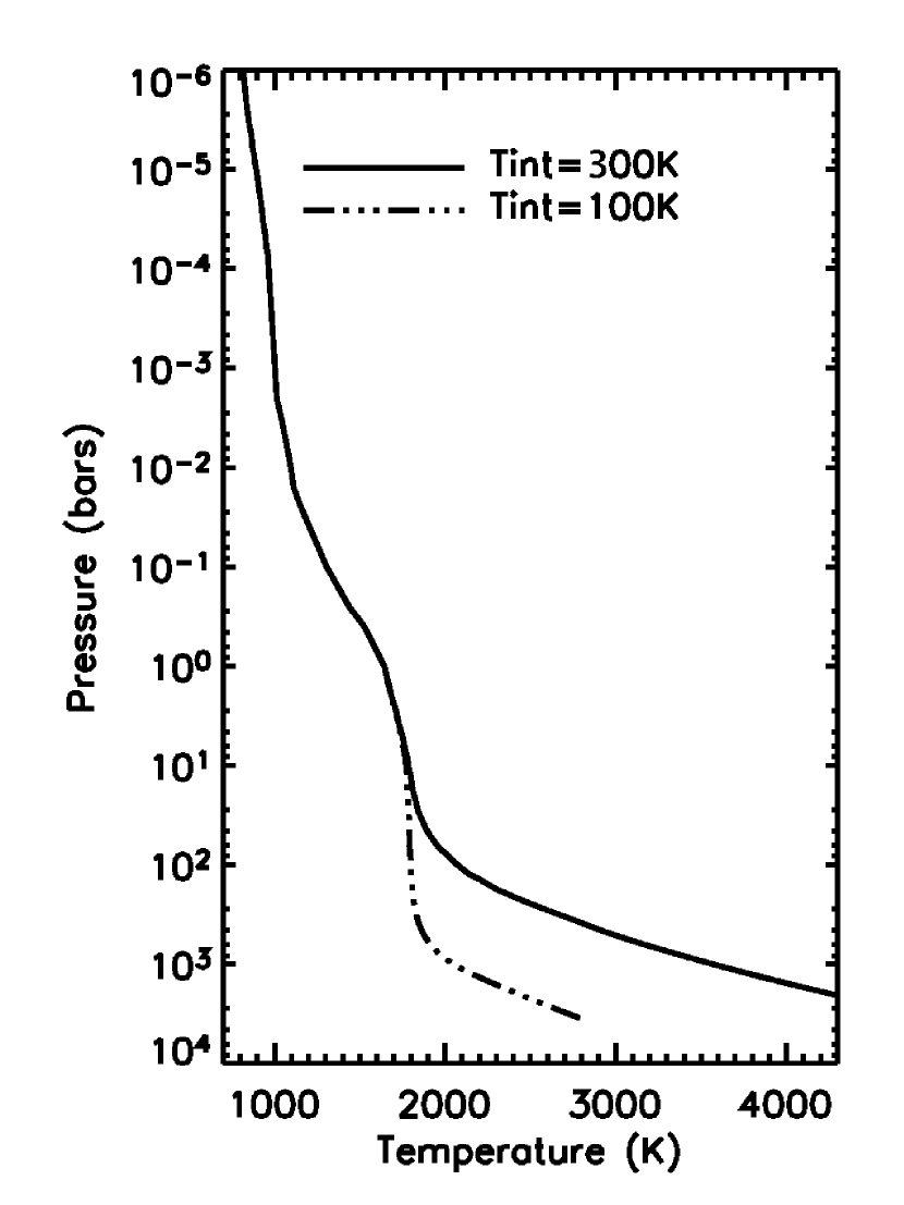
Figure 1: Temperature profiles of the static disk-averaged solutions for the two boundary conditions. There is no difference above the 10–bar level as the intrinsic heat flux becomes negligible with respect to the net stellar flux.

We infer an effective temperature $T_{\rm eff}$ = 1340 and 1350 K for the two boundary conditions (cold and nominal respectively), and a planetary Bond albedo of 0.10. While this albedo closely agrees with that inferred by Baraffe et al. (2003), our $T_{\rm eff}$ is lower because these authors redistribute the stellar flux only over the dayside and thus have a stellar heating twice larger than ours. Below the 3-mbar level, our profile is $\sim$ 600 K cooler than that produced by Sudarsky et al. (2003) (as shown in their Fig. 26). This difference partly results from the twice larger insolation used by these authors who chose the same redistribution of stellar heat as Baraffe et al. (2003). However it can only produce 15-20% larger temperatures as illustrated by Sudarsky et al. (2003)’s comparison of profiles with different incident flux weighting (shown in their Fig. 28). The expected temperature increase below the 3-mbar level is thus limited to 150–300 K. On the other hand, we note that these authors used an intrinsic temperature of the planet of 500 K, hotter than ours, which can contribute to the difference with our model at least below the $\sim$0.5–bar level. Above the 0.3–mbar level, the difference is only $\sim$150 K and can be accounted for by the factor of two in the stellar flux. Another difference between the two models is the incorporation of silicate and iron clouds in Sudarsky et al. (2003)’s model whereas ours is cloud–free. These clouds, with bases at 5–10 mbar in their model, result in a cooler atmosphere below the $\sim$30–mbar level and a hotter atmosphere above, and therefore are not the source of the discrepancy in the lower atmosphere. The (cloud–free) profile calculated by Baraffe et al. (2003) is quasi–isothermal at $\sim$1800 K between 10^-4 and 100 bar whereas ours increases from 1000 to 1800 K for the same $T_{\rm int}$=100 K. Lowering the insolation by half in Baraffe et al. (2003)’s model should bring it down to $\sim$1500 K but cannot produce the gradient we have or the even steeper one of Sudarsky et al. (2003). Below the 0.3–bar region, our profile is intermediate between those of Sudarsky et al. (2003) and Baraffe et al. (2003) after correcting to first order for their twice larger stellar heating.

The preferred boundary condition used by Guillot & Showman (2002) for HD209458b’s radius is: $T(p=3{\rm bar})=T_{\rm isolated}(T_{\rm eff},g)-1000\textrm{ K}$, where $T_{\rm isolated}(T_{\rm eff},g)$ is the temperature of an isolated planet of same effective temperature $T_{\rm eff}$ and gravity $g$ as calculated by Burrows et al. (1997). This is relatively close to our solution profile, which implies a 3–bar temperature that is 1200 K less than in the isolated case.

3.2 Penetration of the stellar flux and spectra

Figure 2 shows the net stellar flux as a function of pressure level for the “cold” and “nominal” profiles. We find that 90% of it is absorbed at the $\sim$0.9-bar level, 99% around the 2-bar level, and 99.99% at the $\sim$7-bar (resp. 5–bar) level in the cold (resp. nominal) case. At this level and deeper, the stellar flux becomes smaller than the intrinsic flux (calculated in the cold case) and cannot affect the temperature profile in a significant way. At deep levels, the stellar flux decreases more rapidly with depth in the nominal case than in the cold case due to the larger abundances of H${}_{2}^{-}$ and H^- ions and of TiO. Guillot & Showman (2002) estimated that a penetration of 1% of the stellar flux to $p\leavevmode\nobreak\ \sim$ 100 bar in the “cold” case would allow the radius of HD209458b to be explained without any other energy dissipation. Clearly our calculations indicate that this is not the case and that the large atmospheric opacity beneath pressure levels of a few bars prevents any significant fraction of the stellar heat from reaching directly the $\sim$100 bar region. Therefore, provided that the error bars on the planet’s radius are not underestimated, we confirm the need for an additional heat source at deep levels as advocated by Bodenheimer et al. (2001), Guillot & Showman (2002) and Baraffe et al. (2003).

Figure 2: Net stellar flux as a function of pressure level for the Cold and Nominal profiles.

The reflected and thermal spectra of the planet are shown in Fig. 3. The thermal spectrum is dominated by the water vapor bands, but CO absorption bands around 2100, 4300, and 6400 cm^-1 are visible. It exhibits spectral windows centered at 2600 cm^-1 (3.8 $\mu$m), 4500 cm^-1 (2.2 $\mu$m), 6000 cm^-1 (1.7 $\mu$m), 7800 cm^-1 (1.28 $\mu$m), and 9400 cm^-1 (1.07 $\mu$m). The most intense one at 3.8 $\mu$m is limited on the short-frequency side by the (1–0) CO band and on the high-frequency side by the $\nu_{3}$ H₂O band. The stellar reflected spectrum peaks around 28 500 cm^-1 (0.35 $\mu$m). At wavenumbers less than $\sim$18 000 cm^-1, it is almost completely absorbed due to weaker Rayleigh scattering and strong atmospheric absorption. In particular, in the region of the alkali lines (13 000–17 000 cm^-1), the flux emitted by the planet is at minimum while that of the star is large. This emphasizes the importance of alkali line absorption in the energy balance of the Pegasides, as first recognized by Burrows et al. (2000).

Figure 3: Reflected and thermal emission spectra of the static disk-averaged solution for the nominal boundary condition, in logarithmic scale. The incident stellar spectrum is shown for comparison.

3.3 Radiative Timescales

To characterize the radiative time constant $\tau_{\rm rad}$ at a given pressure level $p_{0}$, we applied a gaussian perturbation to the radiative equilibrium temperature profile and let it relax to its equilibrium state using Eq. 2. The perturbation has the form $\Delta T(p)=\Delta T_{0}\leavevmode\nobreak\ 2^{-\left[2\ln\frac{p}{p_{0}}\right]^{2}}$, i.e. a full width at half maximum of one scale height. The radiative time constant is calculated from the Newtonian cooling equation:

$$\frac{\Delta T}{\tau_{\rm rad}}=-\frac{\partial(\Delta T)}{\partial t}\quad,$$ (6)

where $\Delta T$ is the temperature deviation from the equilibrium profile at level $p_{0}$. We verified that the Newtonian cooling approximation is justified and yields the same $\tau_{\rm rad}$ as far as $\Delta T_{0}$ is small (typically less than 5% of the equilibrium temperature).

Figure 4: Radiative timescale as a function of pressure level. The symbols show the values of the radiative timescale at 1 bar from Showman & Guillot (2002) (1.1 day; diamond) and that of Cho et al. (2003) (10 days; square).

The result is shown in Fig. 4. As expected, the radiative time constant increases monotically with pressure. Around 1 bar, it is $\sim$2.3 days, about twice the value estimated by Showman & Guillot (2002). On the other hand, the long radiative timescale (10 days) assumed by Cho et al. (2003) implies that they significantly underestimated the cooling in their circulation model.

Above the 1–bar pressure level, the radiative timescale is relatively short – less than the rotation period – and we thus expect a rapid response from the planet’s atmosphere to a possible atmospheric circulation and large horizontal variations of temperature. In particular, at 0.1 bar, $\tau_{\rm rad}$ is 3$\times$10⁴ sec (8 hr). This region, which corresponds to the optical limb of the planet at 0.6 $\mu$m due to Rayleigh scattering, is that probed by the transit observations (Charbonneau et al. 2002). The small radiative time constant suggests that the day–night thermal contrast is large and that the atmospheric morning limb may be significantly colder than the evening one for any reasonable zonal wind speed – as measured in the synchronously–rotating frame –. This likely asymmetry, in temperature and hence potentially in the chemical composition, should be kept in mind when analyzing spectroscopic transits. Below the 1–bar level, the opacity is large and the timescale increases rapidly, varying almost as $p^{2}$. We limited this calculation to 10 bar because below this level our profile becomes convective in the nominal case (Fig. 1) and the radiative timescale then cannot be calculated with the same method.

4 Time-dependent solutions for an atmosphere in solid rotation

4.1 Longitude-dependent temperature profiles

We then introduce a solid body rotation by moving the atmosphere with a constant angular velocity with respect to the synchronously–rotating frame. This procedure mimicks a zonal atmospheric circulation and allows us to investigate the temperature as a function of longitude. The effect of rotation is considered only through the modulation of the incoming stellar flux. The insolation is maximum at the substellar longitude (noon) and constantly decreases until the atmosphere no longer receives the stellar flux on the night side. This periodic insolation is shown in Fig. 5. A first limitation of our model is that heating and cooling rates are valid for layers which are static with respect to each other. The rotation of the atmosphere is thus approximated by a solid body rotation, i.e. with a zonal wind constant with height. A second limitation is that these heating and cooling rates correspond to a given chemical composition (associated with the nominal temperature profile in Fig. 1) that does not change during the integration process.

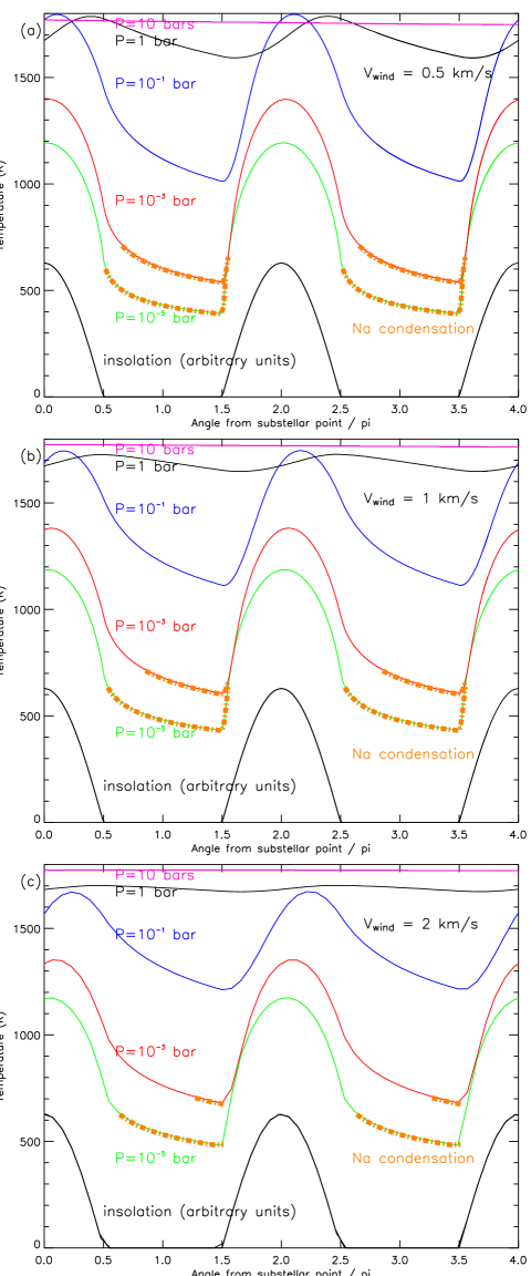
Figure 5: Temperature at selected levels as a function of longitude for an equatorial wind velocity of (a) 0.5 km sec^-1 (b) 1 km sec^-1 and (c) 2 km sec^-1. The incoming insolation is shown in arbitrary units. Note the shift of the maximum of temperature with respect to the maximum of insolation (at the substellar point) as depth (and so the radiative timescale) increases. Below the 10–bar level, the temperature field is essentially uniform.

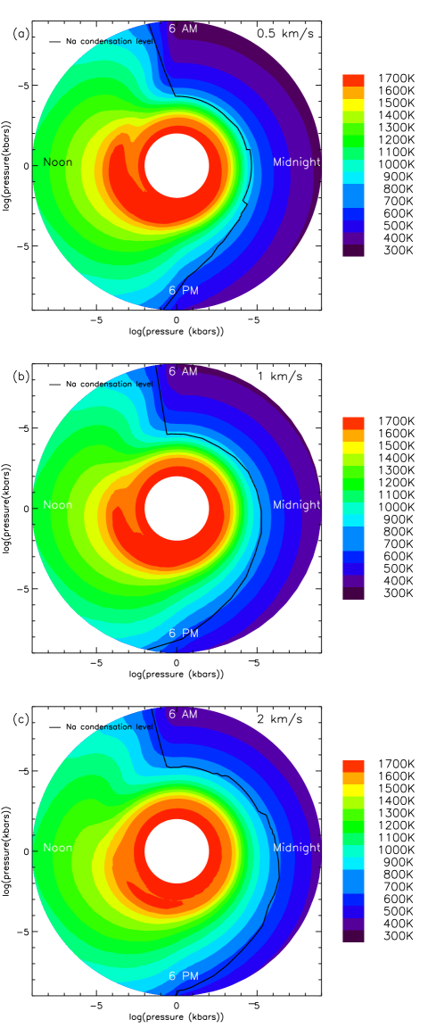
Figure 6: Equatorial cut of the atmosphere between the 1$\times$10^-6 and 10–bar levels for an equatorial wind velocity of (a) 0.5 km sec^-1, (b) 1 km sec^-1, and (c) 2 km sec^-1. The level where condensation of sodium occurs (black line) goes deeper as the night wears on (anti-clockwise) and is deepest at the morning limb . Below 10 bar, the temperature field (not shown here) is uniform and depends only on the bottom boundary condition.

We compute the temperature profiles for rotation periods corresponding to equatorial wind velocities of 0.5, 1 and 2 km sec^-1, in the range predicted by Showman & Guillot (2002). The effective temperature of the planet is shown in Fig. 7 and the temperature at selected levels is displayed in Fig. 5 as a function of longitude. Figure 6 shows an equatorial cut of the atmosphere, with the color scale for temperature indicated on the right. The temperature maximum shifts with respect to the maximum of insolation as depth increases. This phase lag results from the increase in the radiative timescale with depth. It is particularly noticeable at $p\geq$ 1 bar, where $\tau_{\rm rad}$ becomes comparable or exceeds the rotation period. We found day/night temperature variations exceeding 400, 600 and 800 K above the $\sim$0.1–bar level for equatorial winds of 2, 1 and 0.5 km sec^-1 respectively. These values are of the same order as predicted by Showman & Guillot (2002). However, at their reference level of 1 bar and for a wind of 1 km sec^-1, the contrast we get is at most 100 K, less than the $\sim$500 K they predict. Part of the discrepancy comes from the half lower radiative timescale used by these authors. In fact, the temperature contrast estimated by those authors pertains to the level where $T\sim T_{\rm eff}$ which takes place at 0.15 bar in our model, instead of 1 bar. Figure 5 shows that we do get contrasts of 400–700 K in $T_{\rm eff}$ for winds in the range 2–0.5 km sec^-1.

Figure 7: Effective temperatures as a function of longitude for the three wind velocities.

Below the $\sim$5–bar level, the temperature field is essentially uniform with longitude (and time) due to the long radiative timescale. It is then equal to that given by the radiative equilibrium solution under planet–averaged insolation conditions. This points to the need of considering this temperature as a boundary condition for evolutionary models rather than that corresponding to the illuminated hemisphere with no day–to–night redistribution of heat (e.g., Burrows et al. 2003; Baraffe et al. 2003).

An important effect is that the temperature profile becomes cold enough on the night side to allow sodium to condense, as shown in Figs. 5–6. The condensation level extends relatively deep in the atmosphere on the night side and on the morning limb, down to 0.1, 0.3 and 0.5 bar for equatorial wind speeds of 2, 1 and 0.5 km sec^-1 respectively. This is close or even below the optical limb around the Na resonance doublet at 589.3 nm. Hence, during a transit, we expect stellar radiation at this wavelength to be less absorbed on the morning limb than on the evening limb.

4.2 Sodium condensation and transit spectra

Charbonneau et al. (2002) conducted HST spectroscopic observations of HD209458 centered on the sodium resonance doublet at 589.3 nm. Using four planetary transits, they found a visible deeper dimming in a bandpass centered on this feature than in adjacent bands. They interpreted it as absorption from sodium in the planet’s atmosphere. However, the sodium absorption seen in the data is lower than predicted by existing models by approximately a factor three (Hubbard et al. 2001; Brown 2001). These authors invoke several possibilities to explain such a depletion:

• condensation of sodium into mostly Na₂S. However according to their model a very large fraction (99%) of the sodium should condense out to explain by itself such a small absorption.

• Ionization of sodium by the large stellar flux incident on the planetary atmosphere. This is a secondary effect which cannot explain alone the weak absorption, as confirmed by Fortney et al. (2003).

• Very high (above the 0.4-mbar level) particulate opacity. This possibility is difficult to assess as modeling of photochemical hazes still needs to be performed.

• A bulk depletion of the sodium abundance in HD209458. It appears however that parent stars of close-in planets generally have a high metallicity (Gonzalez 1997, 2000).

An alternate explanation is provided by Barman et al. (2002). According to their work, Na could be far from being in local thermodynamic equilibrium in the limb region. This effect would then reduce the depth of the Na absorption seen during a transit. The amplitude of the effect is however difficult to assess due to the lack of well determined collisional deactivation rates from H₂ and He.

It should be noted that the models used to analyze the observations were static and horizontally uniform whereas Charbonneau et al. (2002)’s data pertain to the planetary limb. Horizontal temperature variations due to insolation and dynamics can drive compositional variations that should be taken into account to calculate the sodium abundance over the limb. More specifically, if sodium condenses on the night side, half of the limb is depleted in sodium above some level in the atmosphere. This effect can potentially reduce by half the sodium absorption during a transit compared to the prediction from static models.

We present here calculations of the spectral variation of the planetary radius in the region of the Na lines. The radius $r(\nu)$ is defined here as the limb corresponding to a tangential extinction optical depth of unity. To determine it, we calculate, as a function of frequency, the transmission of the atmosphere for a series of lines of sight at radii $r_{\rm i}(\nu)$ and then interpolate in this grid to find $r(\nu)$. This spectrum $r(\nu)$ is finally convolved to a resolution of 1000. Two models are considered: one, corresponding to the evening limb, incorporates the temperature calculated at a phase of $\pi$/2 (see Fig. 5) and the associated gas profiles; the second one corresponds to the morning limb at a phase of 3$\pi$/2. Results are shown in Fig. 8 for an equatorial wind speed of 1 km sec^-1. As we had anticipated, the Na absorption is much less pronounced in the morning spectrum than in the evening one due to sodium condensation. Integrating the spectra over narrow bands at (588.7–589.9 nm) and around (581.8–588.7 nm and 589.9–596.8 nm) the Na feature as did Charbonneau et al. (2002), we find that the absorption depth is three times weaker on the morning limb ($\delta R_{\rm m}=4.4\times 10^{-3}R$) compared with the evening limb ($\delta R_{\rm e}=1.4\times 10^{-2}R$). During the transit, the stellar spectrum is absorbed by the whole limb (morning and evening) and our model thus predicts a dimming in the sodium band almost half lower than without consensation of Na. We calculate it as $(\delta R_{\rm m}+\delta R_{\rm e})R/R_{\star}^{2})$ = 2.8$\times$10^-4 within the uncertainty range of the observed value (2.32$\pm$0.57$\times$10^-4).

Figure 8: Spectra of the Na lines region for the morning limb (lower) and the evening limb (upper) for a wind velocity of 1 km/s.

5 Conclusions

We have developped a time-dependent one-dimensional radiative model and applied it to the case of HD209458b. Because it is one-dimensional, the model is necessarily simplified in the sense that advection is included only horizontally in the limit of a solid-body rotation of the atmosphere and vertically with convective adjustements of the temperature profile where applicable. Furthermore, important effects such as the possible presence of clouds and time-dependent variations of the absorption coefficients due to variations of the chemical composition are not included. These effects can be considered in a useful way only through a detailed global circulation model, which is beyond the scope of this paper. Conversely, the results of our model can be used as a basis for future dynamical models of the atmosphere of HD209458b and of Pegasides. They also impact evolution calculations and our perception of the vertical and longitudinal structure of strongly irradiated planets, as detailed hereafter.

First, we point out that when considering constant planetary-averaged conditions, our radiative equilibrium profile is colder than those calculated by Sudarsky et al. (2003) and Baraffe et al. (2003) mostly because those authors used a twice larger insolation. After correcting to first order for this difference, our profile agrees with that of Sudarsky et al. (2003) above the $\sim$0.3–mbar region, is still colder than Sudarsky et al. (2003)’s and Baraffe et al. (2003)’s profile down to $\sim$0.3 bar (with a maximum discrepancy of 300–400 K), and is intermediate between these two other models below this region. These remaining differences probably lie in the opacity sources or the radiative transfer treatment but they should not alter the results that follow.

In our model, 99.99% of the stellar flux is absorbed at the 5–bar level (99 % at the 2–bar level). This rapid absorption prevents a significant fraction ($\sim$1 %) of the stellar energy from directly reaching pressure levels of several tens of bars. This mechanism cannot thus supply the energy source required at deep levels to explain the radius of HD209458 (Guillot & Showman 2002; Baraffe et al. 2003).

The radiative timescales that we derive are generally twice longer than those used by Showman & Guillot (2002) and 5 times shorter than assumed by Cho et al. (2003). Above the 1–bar level, the radiative time constant is shorter than the rotation period of the planet. These relatively short values imply that the atmosphere reacts relatively quickly to perturbations from atmospheric dynamics.

In order to qualitatively test the effect of dynamics on the atmospheric structure, we calculated models in which the stellar flux was modulated with a period between 3.5 and 14 days, mimicking the effect of a 0.5– to 2–km s^-1 equatorial zonal jet on an otherwise synchronously rotating planet.

Depending on the imposed wind, we found longitudinal temperature variations to be between 400 and 600 K at 0.1 bar, 30–200 K at 1 bar and less than 5 K at 10 bar. This is generally consistent with the results obtained by Showman & Guillot (2002). On the other hand, the fact that Cho et al. (2003) obtain temperatures on the night side that can be hotter than on the day side is difficult to explain in light of our results. This cannot be ruled out, but would presumably imply a combination of strong meridional and vertical circulation.

The fact that the temperature rapidly becomes uniform with increasing depth implies that the mixing most probably takes place in a relatively shallow layer of the atmosphere. In our simulations, the temperature reached at deep levels is consistent with that of an atmosphere receiving a stellar flux averaged over the whole planet on both the day side and the night side (i.e. 1/4 of the stellar constant at the planet). This is very important for evolution models, as temperature inhomogeneities at deep levels would tend to fasten the cooling compared to homogeneous models with the same absorbed luminosity (Guillot & Showman 2002). On the contrary, some evolution models (Baraffe et al. 2003; Burrows et al. 2003) are calculated from atmospheric boundary conditions that are relevant to the day side only. These models probably overestimate the temperature of the deep atmosphere and therefore the planet’s cooling time.

Finally, the large longitudinal temperature contrast implies that species such as sodium will condense on the night side. Even with no settling, the morning limb (which is coldest) can be strongly depleted in the condensible species. From calculations of transit spectra representative of the morning and evening limbs, we found that the former shows a 3 times weaker sodium absorption than the latter. The Na dimming we calculated through the entire limb is then in agreement with the sodium absorption observed by Charbonneau et al. (2002) during planetary transits.