Bondi Accretion in the Presence of Vorticity

Abstract

The classical Bondi-Hoyle formula gives the accretion rate onto a point particle of a gas with a uniform density and velocity. However, the Bondi-Hoyle problem considers only gas with no net vorticity, while in a real astrophysical situation accreting gas invariably has at least a small amount of vorticity. We therefore consider the related case of accretion of gas with constant vorticity, for the cases of both small and large vorticity. We confirm the findings of earlier two dimensional simulations that even a small amount of vorticity can substantially change both the accretion rate and the morphology of the gas flow lines. We show that in three dimensions the resulting flow field is non-axisymmetric and time dependent. The reduction in accretion rate is due to an accumulation of circulation near the accreting particle. Using a combination of simulations and analytic treatment, we provide an approximate formula for the accretion rate of gas onto a point particle as a function of the vorticity of the surrounding gas.

1 Introduction

Accretion of a background gas by a point-like particle is a ubiquitous phenomenon in astrophysics, occurring on size scales ranging from black holes in galactic nuclei to individual stars or compact objects accreting the winds of their companions. Bondi, Hoyle, and Lyttleton (Hoyle and Lyttleton, 1939, 1940a, 1940b, 1940c; Bondi, 1952) treated this situation by considering the ideal problem of a massive point particle within a uniform gas moving at a constant speed with respect to the particle. For a polytropic gas, the problem is largely characterized by a single dimensionless parameter, the Mach number $\mathcal{M}$, which is defined as the ratio of the gas-particle velocity to the sound speed of the uniform gas. (The ratio of specific heats $\gamma$ also affects the accretion, but its effects are only order unity.) The Bondi-Hoyle formula gives the approximate accretion rate as a function of $\mathcal{M}$, which, in a version updated by Ruffert (1994) and Ruffert and Arnett (1994), is

$$\dot{M}_{\rm BH}=4\pi\rho_{\infty}G^{2}M^{2}c_{\infty}^{-3}\left[\frac{\lambda^{2}+\mathcal{M}^{2}}{\left(1+\mathcal{M}^{2}\right)^{4}}\right]^{1/2}$$ (1)

Here, $\lambda$ is a number of order unity that depends on $\mathcal{M}$ and on the equation of state. For $\mathcal{M}=0$ (Bondi accretion) in an isothermal medium, $\lambda=\exp(1.5)/4\approx 1.1$.

The Bondi-Hoyle formula finds wide application in astrophysics. Our first motivation for exploring this topic is star formation. The competitive accretion picture of star formation posits that protostars form with initially low masses, typically $\raisebox{-2.15277pt}{$\>\stackrel{{\scriptstyle\textstyle<}}{{\sim}}\>$}0.1M_{\odot}$, and grow in mass by accreting unbound gas from the molecular clump in which they form (Bonnell et al., 1997; Bonnell, Bate, and Zinnecker, 1998; Bonnell et al., 2001a, b; Klessen and Burkert, 2000, 2001). The competition for gas is invoked to explain the initial mass function (IMF). This is a process of Bondi-Hoyle accretion, albeit in a turbulent medium, and one ought to be able to use a Bondi-Hoyle-like formula to estimate the rate at which the proposed “seed” protostars would accrete. A second significant area of application is in black holes, particularly the supermassive black holes (SMBHs) at the centers of galaxies. Numerous authors have used the Bondi formula to estimate the rate at which SMBHs accrete, and found that it substantially overestimates the accretion rate (Di Matteo, Carilli, and Fabian, 2001). Proga and Begelman (2003) have argued that rotation may explain the difference between accretion rates estimated from observations and those predicted by the Bondi rate. A third area of application is in accretion rates onto compact objects. Perna et al. (2003) suggest that a combination of rotation and magnetic fields leads to lower accretion rates onto isolated neutron stars than one would estimate using the Bondi formula. They argue that this lowered accretion rate accounts for the unexpectedly small number of isolated neutron stars that have been detected.

Previous authors have considered the problem of hydrodynamic accretion with non-zero vorticity, both analytically (Sparke and Shu, 1980; Sparke, 1982; Abramowicz and Zurek, 1981) and numerically (Fryxell and Taam, 1988; Ruffert, 1997, 1999; Igumenshchev and Abramowicz, 2000; Igumenshchev, Abramowicz, and Narayan, 2000; Proga and Begelman, 2003). Abramowicz and Zurek (1981) analytically treated accretion of gas with non-zero angular momentum onto a black hole. They found that for very low angular momentum the flow pattern is similar to Bondi accretion; the flow is quasi-spherical, it becomes sonic at a radius much larger than the Schwarzschild radius, and the accretion rate is comparable to the Bondi rate. For high angular momentum, the gas forms a disk and the sonic radius in the equatorial plane becomes only a factor of a few times the Schwarzschild radius. The accretion rate is substantially below the Bondi rate. Proga and Begelman (2003) performed two dimensional axisymmetric simulations of the accretion of slowly rotating gas onto a black hole. They find three regimes of accretion. For sufficiently low total angular momentum, the flow is Bondi-like, similar to the pattern Abramowicz and Zurek (1981) predicted. For intermediate total angular momentum, the highest angular momentum gas that cannot accrete forms a dense torus about the black hole. The torus blocks off accretion except through a thin funnel along the poles, reducing the accretion rate to a value roughly independent of the total angular momentum. Finally, for even higher total angular momentum, a centrifugal barrier, coupled with the dense torus, further reduces the accretion rate.

Our goal in this paper is to unify this work by describing the accretion process using a one-parameter family similar to the Bondi-Hoyle-Lyttleton treatment, and to give an analogous formula for the accretion rate as a function of this parameter. We do this using a combination of three-dimensional simulations and analytic treatment. In these two important respects, our work is more complete than previous work. In §2 we give an analytic analysis of the problem, and present our approximate formula. In §3 we describe the computational methodology we use in our simulations, and in §4 we compare the results of our simulations to the analytic theory we put forth. We summarize our conclusions in §5.

2 Analytic Treatment

We consider a point particle accreting in a medium with non-zero vorticity. The simplest case of this, which we treat here, is a medium with constant density and vorticity far from the particle, and where the gas has no net velocity of relative to the particle. Thus, we consider a particle at the origin of our coordinate system, surrounded by a gas whose velocity far from the particle is

$$\mathbf{v_{\infty}}=\omega_{*}c_{\infty}\frac{y}{r_{\rm B}}\hat{x},$$ (2)

where $r_{\rm B}\equiv GM/c_{\infty}^{2}$ is the standard Bondi radius, $M$ is the mass of the particle, $c_{\infty}$ is the sound speed of the gas at infinity, and $y$ is the $y$ coordinate. The factor $\omega_{*}$ is a dimensionless number which we call the vorticity parameter, since the vorticity of the velocity field is $-\omega_{*}c_{\infty}/r_{\rm B}\hat{z}$, independent of position.

The significance of $\omega_{*}$ is clear: $\omega_{*}=1$ corresponds to the case where gas with an impact parameter $y=r_{\rm B}$ is traveling at the sound speed at infinity. The Keplerian velocity at a distance of $r_{\rm B}$ from the central object is

$$v_{K}(r_{\rm B})=\sqrt{\frac{GM}{r_{\rm B}}}=c_{\infty}.$$ (3)

Thus, for $\omega_{*}=1$, gas whose impact parameter is $r_{\rm B}$ is traveling at the Keplerian velocity for that impact parameter. Since $v_{K}\propto r^{-1/2}$, while for our initial velocity field $v_{\infty}\propto y$, gas with smaller impact parameters is sub-Keplerian, while gas with larger impact parameters is super-Keplerian. For $\omega_{*}<1$, the transition from sub- to super-Keplerian $v_{\infty}$ occurs at impact parameters larger than $r_{\rm B}$; for $\omega_{*}>1$, the transition occurs at impact parameters smaller than $r_{\rm B}$. Because the Bondi radius is the distance at which gas comes within the gravitational sphere of influence of the central particle, provided its kinetic energy at infinity is small, we should expect a transition in behavior at $\omega_{*}\approx 1$.

We note that previous authors (e.g. Abramowicz and Zurek (1981); Proga and Begelman (2003)) have usually parameterized their flows in terms of specific angular momentum rather than vorticity, as we do here. The choice of parameterization is somewhat a matter of taste. Specific angular momentum has the advantage that it yields a circularization radius for the flow that depends only on the specific angular momentum, simplifying the analysis. On the other hand, the choice of vorticity enables us to invoke the Kelvin Circulation Theorem in our analysis, which we find helpful. In addition, since specific angular momentum is a function of accretor position, and gas farther than $r_{\rm B}$ from an accretor is unaware of its presence, arranging a flow with constant specific angular momentum requires an unlikely coincidence. It is more natural to characterize a flow by its velocity gradient, hence its vorticity, which is independent of accretor position. Regardless of the choice of parameter, however, it is possible to make an approximate translation of the formulae we derive based on $\omega_{*}$ to ones in terms of the specific angular momentum. For the initial conditions we are considering, the specific angular momentum of a gas parcel with impact parameter $y$ is

$$l_{\infty}=yv_{\infty}=\omega_{*}c_{s}\frac{y^{2}}{r_{\rm B}}.$$ (4)

In the artificial case of a flow with constant specific angular momentum rather than constant vorticity, the equivalent value of $\omega_{*}$ should be determined roughly by the value of the vorticity at the Bondi radius. Thus, as an approximate conversion we suggest $\omega_{*}=l_{\infty}/(c_{s}r_{\rm B})$.

Before moving on to analyze the behavior of accretion as a function of $\omega_{*}$, we consider briefly the question of the gas equation of state. We choose to restrict ourselves to considering an isothermal gas, and we denote the constant sound speed as $c_{s}$. This is physically appropriate for the star formation context: radiative energy transport in the dense molecular gas from which stars form is capable of eliminating any temperature variations on times small compared to the mechanical time scales in the gas (Vázquez-Semadeni et al., 2000). In the context of SMBHs and compact objects, the thermodynamics is more complicated, as the gas can range from isothermal to adiabatic depending on the efficiency of radiative energy transport. However, based on prior simulation work with Bondi accretion (Ruffert, 1994; Ruffert and Arnett, 1994), and accretion with shear (Ruffert, 1997), we do not believe that changes in the equation of state will change either the flow pattern or the accretion rate by more than a factor of order unity.

2.1 Very Small $\omega_{*}$

Abramowicz and Zurek (1981) performed the first detailed analysis of the cases of small and very small $\omega_{*}$ (which we define below), that we shall review and extend. We can distinguish two regimes that occur for $\omega_{*}\ll 1$, depending on the physical dimensions of the accreting object. In the absence of viscosity or other mechanisms of angular momentum transport, a parcel of gas has constant specific angular momentum $l_{\infty}$ as it falls towards the accretor. The orbit of the gas parcel changes from predominantly radial to predominantly tangential at a characteristic circularization radius, where the parcel’s velocity is roughly the Kepler velocity. The specific angular momentum of a parcel of gas in Keplerian rotation at a distance $r$ from the central object is

$$l_{K}(r)=rv_{K}(r)=\sqrt{GMr},$$ (5)

and the circularization radius is therefore determined by the condition $l_{\infty}=l_{K}(r_{\rm circ})$. Equating (4) and (5), a gas parcel at initial impact parameter $y$ has a circularization radius

$$r_{\rm circ}=\omega_{*}^{2}\frac{y^{4}}{r_{\rm B}^{3}}.$$ (6)

If the circularization radius for a given parcel of gas is small compared to the radius of the accretor, $r_{\rm A}$, then that gas will reach the surface of the accretor traveling in a predominantly radial orbit. Its angular momentum, and its vorticity, will therefore be deposited in the central object and will not otherwise affect the flow pattern, leading to an accretion rate approximately equal to the Bondi rate.

In the case of small vorticity, where the velocity of the gas at infinity is small compared to the Keplerian velocity, gas begins to feel the influence of the accretor at a characteristic radius of $r_{\rm B}$. We can therefore distinguish our two regimes based on the relative sizes of $r_{\rm circ}(r_{\rm B})$ and $r_{\rm A}$. If $r_{\rm circ}(r_{\rm B})<r_{\rm A}$, then we are in the case analogous to that of a small circularization radius in a flow with constant specific angular momentum: the gas that reaches the accretor will be on primarily radial orbits, and the accretion rate should be the Bondi rate. The condition for this to occur is

$$\omega_{*}<\omega_{\rm crit}\equiv\sqrt{\frac{r_{\rm A}}{r_{\rm B}}}.$$ (7)

We term the case $\omega_{*}<\omega_{\rm crit}$ “very small $\omega_{*}$.” To get a sense of values of $\omega_{\rm crit}$ in typical cases, consider some of the applications we discussed in the introduction. In a star forming region, a typical accretor mass is $M\sim M_{\odot}$ and a typical sound speed is $c_{s}\sim 0.2$ km s^-1, giving a Bondi radius of $r_{\rm B}\sim 0.1$ pc. A typical protostellar radius is $r_{\rm A}\sim 10^{12}$ cm, so $\omega_{\rm crit}\sim 10^{-3}$. For the SMBH at the center of the Milky Way, $M\approx 3.7\times 10^{6}M_{\odot}$ for the standard distance estimate (Ghez, 2004). The temperature is not constant and depends on the details of radiative processes, but a reasonable estimate for gas far from the black hole is $\sim 10^{7}$ K (Melia, 1994), giving $c_{\infty}\sim\mbox{few}\times 10^{7}$ cm s^-1 and $r_{\rm B}\sim 0.1$ pc. The accretor radius is the Schwarzschild radius $r_{\rm A}=2GM/c^{2}\sim 10^{12}$ cm, so again $\omega_{\rm crit}\sim 10^{-3}$.

Note that this condition $\omega_{*}\raisebox{-2.15277pt}{$\>\stackrel{{\scriptstyle\textstyle<}}{{\sim}}\>$}\omega_{\rm crit}$ for Bondi-like accretion is roughly equivalent to the conditions of Abramowicz and Zurek (1981) and Proga and Begelman (2003) on the specific angular momentum when the accreting object is a non-rotating black hole. In that case, the accretor radius is the Schwarzschild radius, $r_{\rm A}=2GM/c^{2}$, so $\omega_{\rm crit}=\sqrt{2c_{s}/c}$, and the specific angular momentum of gas with impact parameter $y=r_{\rm B}$ is

$$l_{\infty}(r_{\rm B})=\omega_{\rm crit}c_{s}r_{\rm B}=\sqrt{2}r_{\rm A}c.$$ (8)

In their analytical treatment, Abramowicz and Zurek (1981) estimate that the critical specific angular momentum for Bondi-like accretion $l_{\infty}=2r_{\rm A}c$; however, the exact critical value will depend on the details of how the accretion flow joins onto the central object.

2.2 Small $\omega_{*}$

If the vorticity is larger than $\omega_{\rm crit}$, but still small compared to unity, then gas circularizes before it reaches the accretor. The accretor is effectively a point particle, and cannot absorb angular momentum or vorticity from the flow. In this case, Proga and Begelman (2003) have found in their simulations that gas with too much angular momentum to accrete builds up into a torus around the accretor. This thick torus inhibits accretion by blocking off a large part of the solid angle through which streamlines could otherwise reach the accretor.

We can explain the growth of the torus by making a useful analogy to magnetohydrodynamics. The flow at infinity contains a constant vorticity. In regions of the flow that are non-viscous, the Kelvin Circulation Theorem requires that the vorticity contained in an area element of the fluid is constant. This is analogous to flux-freezing in a magnetic medium. The accretor’s gravity drags lines of vorticity in toward the accreting particle. Near the particle, where viscosity may become significant (for example due to magneto-rotational instability in the accretion disk), gas can slip through the vortex lines and reach the accreting object. However, as long as the region of significant viscosity is confined near the accretor, the vortex lines cannot escape. As accretion drags gas inward, vortex lines build up near the accretor, just as magnetic flux would build up in a magnetic flow.

The effect of this vorticity build-up is to increase the rotational velocity in the gas. Consider a circular curve $C$ of radius $r_{C}$ in the $xy$ plane, centered at the origin. The circulation around curve $C$ is the line integral of the velocity,

$$\Gamma=\oint_{C}\mathbf{v}\cdot\mathbf{dl}=r_{C}\int v_{\phi}d\phi,$$ (9)

and by Stokes’ theorem

$$\Gamma=\int_{A}\mbox{\boldmath$\omega$\unboldmath}\cdot\hat{z}\;dA,$$ (10)

where $\omega$ is the vector vorticity at any point in the flow and $A$ is the area inside curve $C$. As a reference state, consider a velocity field with $\mathbf{v}=\mathbf{v}_{\infty}$ everywhere. The accretion process increases vorticity within the curve relative to this reference state, so it must also increase $\Gamma$ and hence the mean rotational velocity $v_{\phi}$ around $C$. Because the vorticity parameter $\omega_{*}<1$, we know that initially $v_{\phi}<v_{K}$ as long as $r_{C}<r_{\rm B}$. However, this analysis shows that $v_{\phi}$ increases with time, so eventually the rotational velocity will become comparable to the Keplerian velocity and a rotationally supported disk must form. The Keplerian velocity is supersonic for all radii smaller than $r_{\rm B}$, and the inflow onto the disk is not purely radial, so the disk will likely develop internal shocks and a time-dependent structure.

The process of vorticity increase near the accretor cannot continue indefinitely. Eventually, inward transport of vorticity by accreting matter must be balanced by an outward flow of vorticity in gas leaving the vicinity of the accretor and escaping to infinity. The radius at which gas becomes unbound from the accretor and can start escaping is $r_{\rm B}$, and we therefore expect that the disk will extend out to $\sim r_{\rm B}$ in radius. The scale height of a thin Keplerian disk is

$$H=\frac{c_{s}}{\Omega}=c_{s}\sqrt{\frac{r^{3}}{GM}}=r\sqrt{\frac{r}{r_{\rm B}}},$$ (11)

where $\Omega$ is the angular velocity. Since the disk radius is $\sim r_{\rm B}$, we expect $H\sim r_{\rm B}$. Thus, the scale height is comparable to the radius and we have, rather than a disk, a thick torus. The torus may be somewhat thicker for an equation of state with ratio of specific heats $\gamma$ greater than unity, because in that case the sound speed will increase inside the Bondi radius due to compressional heating. However, the compression should be is only order unity at $r\sim r_{\rm B}$, so the effect of compression on the torus scale height should also be order unity.

The circulation trapped within the torus should be

$$\Gamma\sim 2\pi r_{\rm B}v_{K}(r_{\rm B})=2\pi c_{s}r_{\rm B}.$$ (12)

In our reference state with $\mathbf{v}=\mathbf{v}_{\infty}$ everywhere, the circulation is

$$\Gamma_{0}=\pi r_{\rm B}^{2}\omega=\pi c_{s}r_{\rm B}\omega_{*},$$ (13)

which is clearly much smaller than the equilibrium value of $\Gamma$ for $\omega_{*}\ll 1$. The time required for the circulation to build up to $\Gamma$ is determined by the rate at which mass falling onto the accreting object carries vorticity inwards. The gas within the Bondi radius reaches the central object, or the growing disk, on the Bondi time scale, $t_{\rm B}\equiv r_{\rm B}/c_{s}$. Thus, the flow replaces the gas within the Bondi radius on this time scale. Each set of “replacement” gas carries the same vorticity as the gas it is replacing, and therefore increases the circulation by $\Gamma_{0}$. As a result, the time required for the accumulating vorticity to reach its equilibrium value is approximately

$$t_{\rm eq}\sim\frac{\Gamma}{\Gamma_{0}}t_{\rm B}=\frac{2}{\omega_{*}}t_{\rm B}.$$ (14)

This estimate only applies for $\omega_{*}\raisebox{-2.15277pt}{$\>\stackrel{{\scriptstyle\textstyle<}}{{\sim}}\>$}1$, when accumulation of circulation is the key factor in setting the final accretion rate.

We can roughly estimate the amount by which the accretion rate will be reduced by the presence of the torus once the flow reaches equilibrium. The torus reduces accretion by blocking off solid angle through which material could otherwise accrete. If the torus extends out to $r_{\rm B}$, and its height is roughly $r_{\rm B}$ as well, it blocks all angles in the range $\pi/4<\theta<3\pi/4$. If the reduction in accretion rate is proportional to the fraction of solid angle blocked, then the accretion rate for this case should be reduced to $\sim 30\%$ of the Bondi rate, $\dot{M}_{\rm B}$, given by equation (1) for $\mathcal{M}=0$.

It is important to note that the equilibrium state we describe here does not depend on the value of $\omega_{*}$, as long as $\omega_{\rm crit}<\omega_{*}\ll 1$. The equilibrium radius of the torus depends only on the maximum vorticity that can accumulate near the accretor before the velocity becomes comparable to the Kepler velocity and halts infall in the disk. Thus, the equilibrium radius of the torus is $\sim r_{\rm B}$ independent of $\omega_{*}$, and the scale height and accretion rate are also $H\sim r_{\rm B}$ and $\dot{M}\sim 0.3\dot{M}_{\rm B}$, respectively. Different values of $\omega_{*}$ only mean that vorticity builds up more or less slowly, and thus that there is a longer or shorter initial transient.

2.3 Large $\omega_{*}$

The final case to consider is $\omega_{*}\raisebox{-2.15277pt}{$\>\stackrel{{\scriptstyle\textstyle>}}{{\sim}}\>$}1$. In this regime, the velocity of the gas at the Bondi radius is comparable to or larger than the Keplerian velocity. To derive an approximate accretion rate, we adopt an ansatz from Bondi-Hoyle accretion.

Regardless of its velocity, gas at infinity initially has a positive total energy. Its potential energy is zero and it has non-zero internal energy. In order to become bound and accrete onto the point mass, the gas must lose its energy by shocking. If gas does shock, it is likely to accrete. Since the flow at infinity is laminar, shocks will only occur for those streamlines that are bent significantly by the gravity of the accreting particle. To determine if a straight streamline is susceptible to bending, we can compare the velocity of gas on that streamline (adding both bulk and thermal velocity) to the maximum value of the escape velocity along that streamline. If the peak escape velocity is larger, then the streamline will bend and is likely to terminate in a shock. Suppose the gas at infinity is traveling in the $x$ direction, and consider a streamline that begins at $xyz$ coordinates $(\pm\infty,y,z)$. The streamline will bend significantly and pass through a shock if

$$\frac{2GM}{\sqrt{y^{2}+z^{2}}}>v_{\infty}(y,z)^{2}+c_{s}^{2}.$$ (15)

In the Bondi-Hoyle case, $v_{\infty}=\mathcal{M}c_{s}$ independent of $y$ and $z$. Thus, (15) reduces to

$$\sqrt{y^{2}+z^{2}}<\frac{2GM}{c_{s}^{2}(1+\mathcal{M}^{2})}\equiv 2r_{\rm BH},$$ (16)

where we have used the standard definition for the Bondi-Hoyle radius.

If we make the assumption that all parcels of gas traveling on streamlines that bend significantly go through shocks, and all gas that shocks loses enough energy to become bound and eventually reach the accretor, then the rate at which mass accretes onto the particle is equal to the rate at which gas from infinity begins traveling on streamlines that meet condition (15). We can therefore define an area $A$ in the plane at infinity that satisfies (15) and approximate the accretion rate by

$$\dot{M}\approx\int_{A}\rho_{\infty}\sqrt{v_{\infty}(y,z)^{2}+c_{s}^{2}}\;dy\,dz,$$ (17)

where $\rho_{\infty}$ is the density of the gas at infinity and we have again added the bulk and thermal velocities of the gas in quadrature. For the Bondi-Hoyle case, $A$ is simply a circle of radius of radius $2r_{\rm BH}$ and $v_{\infty}$ is a constant, so the integral is trivial. Evaluating it gives

$$\dot{M}_{\rm BH}\approx 4\pi r_{\rm BH}^{2}\rho_{\infty}c_{s}\sqrt{1+\mathcal{M}^{2}}=4\pi\rho_{\infty}\frac{(GM)^{2}}{c_{s}^{3}\left(1+\mathcal{M}^{2}\right)^{3/2}},$$ (18)

which is just the Bondi-Hoyle formula (equation 1) up to factors of order unity.

Because this ansatz allows us to reproduce the Bondi-Hoyle formula, we will apply it to predict the case of accretion with vorticity. In this case, $v_{\infty}=\omega_{*}c_{s}y/r_{\rm B}$, so (15) becomes

$$\frac{2GM}{\sqrt{y^{2}+z^{2}}}>\left(\omega_{*}\frac{c_{s}}{r_{\rm B}}\right)^{2}y^{2}+c_{s}^{2}.$$ (19)

With the convenient change of variable $y^{\prime}=y/r_{\rm B}$ and $z^{\prime}=z/r_{\rm B}$, this becomes

$$2>\left(y^{\prime 2}+z^{\prime 2}\right)^{1/2}\left(1+\omega_{*}^{2}y^{\prime 2}\right).$$ (20)

We can solve (20) for $z^{\prime}$ to find the function $Z^{\prime}(y^{\prime},\omega_{*})$ that defines the boundary:

$$Z^{\prime}(y^{\prime},\omega_{*})=\frac{\sqrt{4-y^{\prime 2}(1+\omega_{*}^{2}y^{\prime 2})^{2}}}{1+\omega_{*}^{2}y^{\prime 2}}.$$ (21)

We refer to region of the $yz$ plane bounded by $\pm Z^{\prime}(y^{\prime},\omega_{*})$ as $A(\omega_{*})$. The maximum value of $y^{\prime}$ on the boundary of $A(\omega_{*})$ occurs for $z^{\prime}=0$, and is

$$y^{\prime}_{\rm max}(\omega_{*})=\frac{3^{1/3}\left(9\omega_{*}+\sqrt{3+81\omega_{*}^{2}}\right)^{2/3}-3^{2/3}}{3\omega_{*}\left(9\omega_{*}+\sqrt{3+81\omega_{*}^{2}}\right)^{1/3}}.$$ (22)

Figure 1 shows the boundary of $A(\omega_{*})$ as a function of $\omega_{*}$.

The approximate accretion rate is

$$\dot{M}(\omega_{*}) \approx r_{\rm B}^{2}\rho_{\infty}c_{s}\int_{A(\omega_{*})}\sqrt{1+\omega_{*}^{2}y^{\prime 2}}\;dy^{\prime}\;dz^{\prime}$$ (23)

$$\equiv 4\pi r_{\rm B}^{2}\rho_{\infty}c_{s}f(\omega_{*}),$$ (24)

where we have defined the numerical factor

$$f(\omega_{*}) = \frac{1}{4\pi}\int_{A(\omega_{*})}\sqrt{1+\omega_{*}^{2}y^{\prime 2}}\;dy^{\prime}\;dz^{\prime}\;$$ (25)

$$= \frac{1}{\pi}\int_{0}^{y^{\prime}_{\rm max}(\omega_{*})}\sqrt{1+\omega_{*}^{2}y^{\prime 2}}\int_{0}^{Z^{\prime}(y^{\prime},\omega_{*})}dz^{\prime}\;dy^{\prime}$$ (26)

$$= \frac{1}{\pi}\int_{0}^{y^{\prime}_{\rm max}(\omega_{*})}\sqrt{\frac{4-y^{\prime 2}(1+\omega_{*}^{2}y^{\prime 2})^{2}}{1+\omega_{*}^{2}y^{\prime 2}}}dy^{\prime}.$$ (27)

The integral is straightforward to evaluate numerically, and we plot the result in Figure 2. We can also obtain an approximation for $f(\omega_{*})$ in the limit $\omega_{*}\rightarrow\infty$. We show in Appendix A that in the limit $\omega_{*}\gg 1$, we can approximate $f(\omega_{*})$ by

$$f(\omega_{*})\approx\frac{2}{3\pi\omega_{*}}\ln\left(16\omega_{*}\right).$$ (28)

We also show this approximation in Figure 2.

We must make one further modification to our estimated accretion rate. In the limit $\omega_{*}\rightarrow 0$, $f(\omega_{*})\rightarrow 1$ and (24) reduces to approximately $\dot{M}_{\rm B}$. Thus, this approximation smoothly interpolates between the cases $\omega_{*}\ll 1$ and $\omega_{*}\raisebox{-2.15277pt}{$\>\stackrel{{\scriptstyle\textstyle>}}{{\sim}}\>$}1$. However, we have already seen that even in the case $\omega_{*}\ll 1$ the accretion rate can be substantially below the Bondi rate, since the accumulation of circulation leads to the formation of a thick torus that blocks streamlines from reaching the accretor. The same phenomenon should happen with $\omega_{*}\raisebox{-2.15277pt}{$\>\stackrel{{\scriptstyle\textstyle>}}{{\sim}}\>$}1$. Circulation will still accumulate near the accretor. The shape of the torus should be the same as in the $\omega_{*}\ll 1$ case, because that is set just by the physics of disks. We therefore reduce our estimated accretion rate (24) by a constant factor so that it matches our estimate of $0.3\dot{M}_{\rm B}$ for the case $\omega_{\rm crit}<\omega_{*}\ll 1$. The required factor is $0.34$; it is not exactly 0.3 because (24) for $\omega_{*}\ll 1$ differs from the Bondi rate by a small factor.

With this modification in place, (24) should give a good approximation of the accretion rate for all $\omega_{*}>\omega_{\rm crit}$. Our final estimate for the accretion rate by a flow with vorticity $\omega_{*}$ at infinity is

$$\dot{M}(\omega_{*})\approx 4\pi\rho_{\infty}\frac{(GM)^{2}}{c_{s}^{3}}\cdot\left\{\begin{array}[]{r@{\quad:\quad}l}\exp(1.5)/4&\omega_{*}<\omega_{\rm crit}\\ 0.34\,f(\omega_{*})&\omega_{*}>\omega_{\rm crit}\end{array}.\right.$$ (29)

In §5 we give a more accurate approximation that is calibrated by our simulations.

3 Computational Methodology

To test the theory presented in the previous section, we ran a series of simulations. In this section, we describe the simulation methodology, and in the next we compare the simulation results to our theory.

3.1 Code

The calculations in this paper use our three dimensional adaptive mesh refinement (AMR) code to solve the Euler equations of compressible gas dynamics

$$\frac{\partial\rho}{\partial t}+\nabla\cdot\left(\rho\mathbf{v}\right) = 0$$ (30)

$$\frac{\partial}{\partial t}\left(\rho\mathbf{v}\right)+\nabla\cdot\left(\rho\mathbf{vv}\right) = -\nabla P-\rho\nabla\phi$$ (31)

$$\frac{\partial}{\partial t}\left(\rho e\right)+\nabla\cdot\left[\left(\rho e+P\right)\mathbf{v}\right] = \rho\mathbf{v}\cdot\nabla\phi,$$ (32)

where $\rho$ is the density, $\mathbf{v}$ is the vector velocity, $P$ is the thermal pressure (equal to $\rho c_{s}^{2}$ since we adopt an isothermal equation of state), $e$ is the total non-gravitational energy per unit mass, and $\phi$ is the gravitational potential. The code solves these equations using a conservative high-order Godunov scheme with an optimized approximate Riemann solver (Toro, 1997). The algorithm is second-order accurate in both space and time for smooth flows, and it provides robust treatment of shocks and discontinuities. Although the code is capable of solving the Poisson equation for the gravitational field $\phi$ of the gas based on the density distribution, in this work we neglect the gas self-gravity and include only the gravitational force of the central object. The potential is therefore

$$\phi=\frac{GM}{r},$$ (33)

where $M$ is the mass of the central object and $r$ is the distance from it. We do not adopt the Paczyński and Wiita (1980) potential frequently used for simulations involving black holes because we are do not wish to limit ourselves to the case of black holes, and because even in the black hole case we are interested in the regime where the Schwarzschild radius is extremely small on scales of the grid, so that general relativistic effects are not important.

Our code operates within the AMR framework (Berger and Oliger, 1984; Berger and Collela, 1989; Bell et al., 1994), and is described in detail in Truelove et al. (1998) and Klein (1999). We discretize the problem domain onto a base, coarse level, denoted level 0. We dynamically create finer levels, numbered $1,2,\ldots n$, recursively nested within one another. To take a time step, one advances level $\mathrm{𝟎}$ through a single time step $\Delta t_{0}$, and then advances each subsequent level for the same amount of time. Each level has its own time step, and in general $\Delta t_{l+1}<\Delta t_{l}$, so after advancing level 0 we must advance level 1 through several steps of size $\Delta t_{1}$, until it has advanced a total time $\Delta t_{0}$ as well. In all the simulations we present in this paper, we chose cell spacings such that $\Delta t_{l}=2\Delta t_{l+1}$, and thus we take two time steps on level 1 for each time step on level 0. (We find that refining by factors of two gives better accuracy in the solution than using a larger refinement factor.) After each level 0 time step, we apply a synchronization procedure to guarantee conservation of mass, momentum, and energy across the boundary between levels 0 and 1. However, each time we advance level 1 through time $\Delta t_{1}$, we must advance level 2 through two steps of size $\Delta t_{2}$, and so forth to the finest level present.

On the finest level of refinement, we represent the central, accreting object with a sink particle (Krumholz, McKee, and Klein, 2004). One noteworthy feature of our sink particle, which we shall discuss further in §3.3, is that the sink particle does not accrete any angular momentum from the gas in the computational grid. This is in contrast the sink methodologies used by previous authors (e.g. Ruffert (1997); Proga and Begelman (2003)), where the sink could accrete angular momentum as well as mass. Our approach is appropriate for $\omega_{*}\gg\omega_{\rm crit}$, which is the case on which we focus.

3.2 Initial and Boundary Conditions

For each run, we place a sink particle at the origin of an initially uniform gas. The gas has an initial velocity field

$$\mathbf{v_{0}}=\omega_{*}c_{s}\frac{y}{r_{\rm B}}\hat{x},$$ (34)

where we use different values of $\omega_{*}$ in different runs. Table 1 summarizes the values of $\omega_{*}$ that we simulated. Our computational domain extends from $-100r_{\rm B}$ to $100r_{\rm B}$ in the $x$ and $z$ directions. In the $y$ direction, we also used a range of $-100r_{\rm B}$ to $100r_{\rm B}$ for smaller values of $\omega_{*}$. For larger values of $\omega_{*}$, though, the large velocities that occur at large values of $y$ produce very small time steps that make the computation prohibitively expensive. We therefore use a smaller domain in the $y$ direction, as we indicate in Table 1; in every case, however, we chose our domain to extend to values of $y$ such that $v_{0}(y_{\rm max})\gg v_{\rm escape}(y_{\rm max})$.

We used inflow/outflow boundary conditions in the $x$ direction and symmetry in the $y$ and $z$ directions. However, for all our runs the boundary is sufficiently far away from the central object that, within the duration of the run, no sound waves can propagate from the central object to the boundary and back. Our lowest resolution runs have $\Delta x_{\rm min}<r_{\rm B}/40$, which we use for smaller values of $\omega_{*}$. For larger values of $\omega_{*}$, we use $\Delta x_{\rm min}<r_{\rm B}/160$. We set up our adaptive grids such that, at any radius $r$, the local grid resolution is $\Delta x\leq\max(r/20,\Delta x_{\rm min})$.

3.3 The Sink Particle Method and Very Small Vorticity

As Table 1 indicates, we vary $\omega_{*}$ from $10^{-2}$ to $10^{1.5}$, thereby thoroughly exploring the small $\omega_{*}$ and large $\omega_{*}$ regimes. However, none of our work explores the very small $\omega_{*}$ regime. This is for two reasons, one physical and one technical. In order to explore the very small $\omega_{*}$ case, one must use either an unphysically small value of $\omega_{*}$ or an unphysically large accretor radius, leading to an unrealistically large $\omega_{\rm crit}$. As we have shown in §2.1, for typical astrophysical situations in which accretion with vorticity is important, $\omega_{\rm crit}\sim 10^{-3}$. This is a truly tiny amount of vorticity, corresponding to a shear of one thousandth of the sound speed at one Bondi radius. In the case of a protostar in a molecular clump, this corresponds to a velocity gradient of no more than $\sim 10$ cm s^-1 over a distance of $\sim 0.1$ pc; for the galactic center, it corresponds to a gradient of $\sim 10^{4}$ cm s^-1 over a distance of $\sim 0.1$ pc. It is difficult to see how to produce such an irrotational flow field, and thus the very small $\omega_{*}$ case is not relevant for the applications with which we are concerned.

The technical reason we do not treat the very small $\omega_{*}$ case is that our sink particle method is constructed to exactly conserve total angular momentum during the accretion process. (For details, see Krumholz, McKee, and Klein (2004).) Transfer of vorticity from the flow to the accretor is the distinguishing characteristic of flow with $\omega_{*}<\omega_{\rm crit}$. However, since our sink particle does not change the angular momentum of the flow field, it actually increases vorticity by removing mass while leaving angular momentum. Our code does dissipate vorticity via numerical viscosity, as we discuss in more detail in §4.4 on convergence testing. However, this effect is small except in the inner few zones. On balance, we consider this approach more realistic than the standard technique of allowing any angular momentum that enters a chosen accretion region to accrete. In reality, a small accretor should absorb negligible angular momentum from the flow on scales much larger than the accretor radius. In real accretion disks, viscosity acts to transfer mass inwards and angular momentum outwards. This is exactly the approximation we adopt in our sink particle method: mass travels inwards, angular momentum does not. While ideally one would follow the flow down to the true physical surface of the accretor, this is computationally infeasible in more than one dimension even with AMR. Our sink particle method provides a more realistic approximation of the behavior of an accretion disk than would allowing angular momentum to accrete.

4 Simulation Results

4.1 Density and Velocity Fields

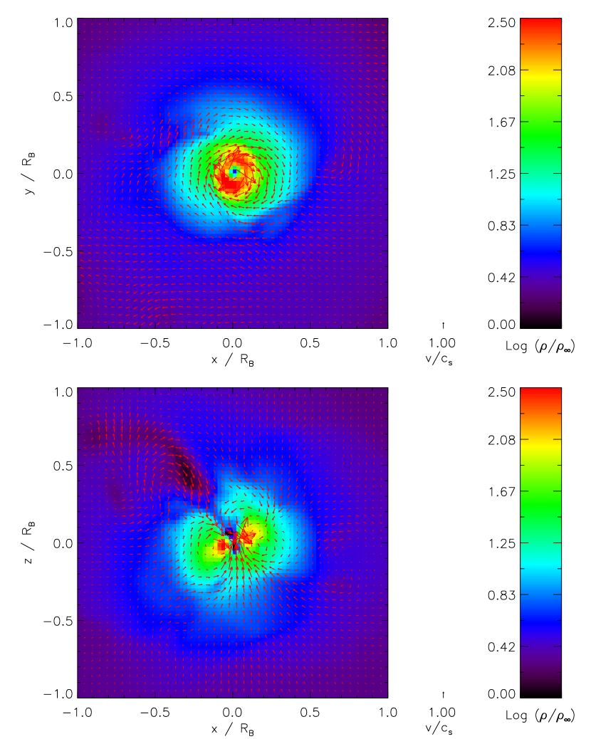
Figure 3: The plots show slices through the origin in the $xy$ and $xz$ planes for the $\omega_{*}=10^{-2}$ run. The grayscale indicates log density, and the arrows indicate velocity. Note the differences in scale from Figures 4 and 5.

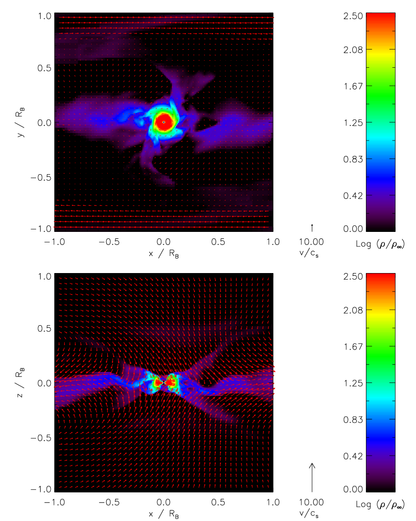
Figure 4: The plots show slices through the origin in the $xy$ and $xz$ planes for the $\omega_{*}=1$ run. The grayscale indicates log density, and the arrows indicate velocity. Note the differences in scale from Figures 3 and 5.

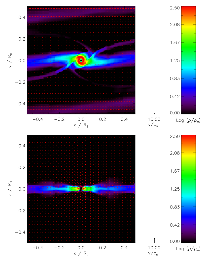
Figure 5: The plots show slices through the origin in the $xy$ and $xz$ planes for the $\omega_{*}=10^{1.5}$ run. The grayscale indicates log density, and the arrows indicate velocity. Note the differences in scale from Figures 3 and 4.

In each of the simulations, the flow went through a transient and then settled down into a quasi-equilibrium state. The time required to reach equilibrium increased with decreasing $\omega_{*}$, ranging from $\sim 100t_{\rm B}$ for $\omega_{*}=10^{-2}$ to $\sim t_{\rm B}$ for $\omega_{*}\raisebox{-2.15277pt}{$\>\stackrel{{\scriptstyle\textstyle>}}{{\sim}}\>$}1$, where $t_{\rm B}\equiv r_{\rm B}/c_{s}$ is the Bondi time. In the equilibrium configuration, all the runs except $\omega_{*}=0$ built up dense material around the accretor. The material was not in a symmetric disk, but rather in a pinwheel shape. The velocity patterns associated with these pinwheels generally involved matter flowing in from the $z$ direction through an accretion funnel and either circulating or outflowing in the $xy$ plane. This overall morphology agrees well with the results of Proga and Begelman (2003). Figures 3, 4, and 5 illustrate the morphology for $\omega_{*}=10^{-2}$, 1, and $10^{1.5}$.

A comparison of runs at different $\omega_{*}$ values shows several clear trends. First, the accumulated pinwheel of matter is much smaller at large $\omega_{*}$ than at small $\omega_{*}$. For $\omega_{*}\raisebox{-2.15277pt}{$\>\stackrel{{\scriptstyle\textstyle<}}{{\sim}}\>$}1$, the accumulated matter extends out to $\sim r_{\rm B}/2$, while for $\omega_{*}\gg 1$ it is well inside the Bondi radius and is less massive. The size of the pinwheel changes only slightly with $\omega_{*}$ for $\omega_{*}\raisebox{-2.15277pt}{$\>\stackrel{{\scriptstyle\textstyle<}}{{\sim}}\>$}1$, but shrinks dramatically for $\omega_{*}\raisebox{-2.15277pt}{$\>\stackrel{{\scriptstyle\textstyle>}}{{\sim}}\>$}1$. Our theoretical description of the torus we expect for small $\omega_{*}$ appears to be roughly correct: a torus of material accumulates that extends out to $\sim r_{\rm B}$ and has a height comparable to its radius. The tori are chaotic and time-variable. For larger $\omega_{*}$, the pinwheels are more regular and less chaotic, and are accompanied by leading and trailing shocks. The shocks are moderately strong, with Mach numbers $\sim 2-3$.

For $\omega_{*}\raisebox{-2.15277pt}{$\>\stackrel{{\scriptstyle\textstyle<}}{{\sim}}\>$}1$, we do not find that the torus has constant specific angular momentum, as Proga and Begelman (2003) did. In our torii, the specific angular momentum of the gas varies by orders of magnitude. It is unclear if this difference in results is due to different initial conditions, or due to the fact that our simulations are three-dimensional where theirs were two-dimensional. However, we agree with Proga and Begelman (2003) that the size and shape of the torus is largely independent of $\omega_{*}$ (or the initial specific angular momentum $l$), and that its equilibrium structure arises due to the accumulation of material with too much vorticity (or $l$) to accrete. As Figures 3 and 4 show, accretion occurs only through a narrow funnel, and the (invariant) shape of the torus therefore determines the accretion rate.

4.2 Evolution of Circulation

For each run we computed the average dimensionless circulation $\Gamma$ as a function of time. We define the dimensionless circulation within a circle of radius $r_{\rm B}$ in the $xy$ plane as

$$\Gamma_{*}=-\frac{1}{\pi r_{\rm B}c_{s}}\oint_{r=r_{\rm B}}\mathbf{v}\cdot\mathbf{dl},$$ (35)

where the line integral is evaluated on the circle $r=r_{\rm B}$. The circulation is a measure of the amount of vorticity within one Bondi radius of the accretor. With this definition of dimensionless circulation, in the initial configuration of the velocity field the circulation is equal to the vorticity parameter, $\Gamma_{*}=\omega_{*}$. Our prediction for the equilibrium circulation for $\omega_{*}\raisebox{-2.15277pt}{$\>\stackrel{{\scriptstyle\textstyle<}}{{\sim}}\>$}1$ is $\Gamma\sim 2\pi c_{s}r_{\rm B}$, or $\Gamma_{*}\sim 2$.

We plot the circulation versus time along with the accretion rate versus time for each of our runs in Figure 6. The behavior of the circulation with time depends on the value of $\omega_{*}$. For $\omega_{*}\raisebox{-2.15277pt}{$\>\stackrel{{\scriptstyle\textstyle<}}{{\sim}}\>$}1$, the circulation starts at $\omega_{*}$ and gradually increases until it reaches $\sim 0.4-0.8$. Then it fluctuates around this mean. For $\omega_{*}=10^{0.5}$, $\Gamma_{*}$ decreases from its initial value until it again reaches the range $\sim 0.4-0.8$. As $\omega_{*}$ increases, however, $\Gamma_{*}$ decreases less and less in the time it takes the accretion rate to reach equilibrium. The accretion rate and the circulation appear to be anti-correlated for $\omega_{*}\raisebox{-2.15277pt}{$\>\stackrel{{\scriptstyle\textstyle<}}{{\sim}}\>$}1$ in the period before equilibration: the initial buildup of circulation takes about the same amount of time as the initial decrease in the accretion rate. This supports our hypothesis that vortex lines are acting like magnetic flux lines and inhibiting accretion.

For each run we estimate by eye the time at which the flow pattern and accretion rate reach equilibrium, and we compute the mean circulation after this time. We report the equilibration times and the mean circulations in Table 1; we plot the equilibrium value of $\Gamma_{*}$ in Figure 7, and the equilibration time in Figure 8. As the figures show, the equilibrium value of the circulation is at most very weakly dependent on the initial vorticity for $\omega_{*}\raisebox{-2.15277pt}{$\>\stackrel{{\scriptstyle\textstyle<}}{{\sim}}\>$}1$, varying by less than a factor of 2 while the initial vorticity varies by a factor of 100. The flow pattern re-arranges itself to select $\Gamma\sim 0.4-0.8$ by accumulating a dense torus of material rotating at nearly Keplerian speeds around the accretor. The equilibrium value is smaller than our prediction of $\Gamma_{*}\sim 2$, indicating that the rotational velocity is sub-Keplerian. This result is consistent with the morphology of the gas flow. The gas has a non-zero radial velocity and thus can be marginally bound even with tangential velocities that are sub-Keplerian. Our analytic model, because it fails to predict the chaotic nature of the flow pattern, overestimates the equilibrium value of $\Gamma_{*}$ by a factor of $\sim 4$. It does, however, correctly predict that there is an equilibrium $\Gamma_{*}$ for $\omega_{*}\raisebox{-2.15277pt}{$\>\stackrel{{\scriptstyle\textstyle<}}{{\sim}}\>$}1$. At $\omega_{*}\raisebox{-2.15277pt}{$\>\stackrel{{\scriptstyle\textstyle>}}{{\sim}}\>$}1$, the pinwheel of unaccreted matter is confined closer to the accretor, and is unable to affect the circulation on length scales $\sim r_{\rm B}$. Thus, the circulation for larger $\omega_{*}$ stays constant.

The equilibration time is also roughly consistent with our prediction of $t_{\rm eq}=2t_{\rm B}/\omega_{*}$ for $\omega_{*}\raisebox{-2.15277pt}{$\>\stackrel{{\scriptstyle\textstyle<}}{{\sim}}\>$}1$. Part of the scatter of the line comes from the unavoidable subjectivity in our estimate of the equilibration time in such a chaotic flow. However, our model is clearly only approximate. While we correctly capture the trend of increasing equilibration time with decreasing $\omega_{*}$, our inability to model the turbulent flow means that our prediction of the equilibration time, like our prediction of $\Gamma_{*}$, is accurate to at best a factor of a few.

In the plots of $\Gamma_{*}$ and $t_{\rm eq}$ versus $\omega_{*}$ (and as we show below, in the plot of $\dot{M}$ versus $\omega_{*}$ as well), there seems to be a change in behavior between the $\omega_{*}=10^{-1}$ and $\omega_{*}=10^{-0.5}$ runs. Rather than smoothly interpolating bewteen $\omega_{*}\ll 1$ and $\omega_{*}\gg 1$, the trend with $\omega_{*}$ appears to jump from one track to another. We cannot rule out the possibility that this is simply the result of chance and our sparse sampling $\omega_{*}$ values. Near $\omega_{*}=1$, the equilibrium values of quantities like $\Gamma_{*}$ and $t_{\rm eq}$ may be fluctuating chaotically with $\omega_{*}$, and the sharp jump we see from $\omega_{*}=10^{-1}$ to $\omega_{*}=10^{-1/2}$ may just be a fluctuation. However, it is also possible that there is a distinct regime of intermediate $\omega_{*}$, as well as the small and large $\omega_{*}$, and that several properties of the equilibrium flow change suddenly when one enters this new regime.

4.3 Accretion Rates and Comparison to Theory

We ran each of our simulations until the accretion rate converged to a steady state, and then we measured both the mean accretion rate and the fluctuations about the mean. Table 1 summarizes our results and Figure 6 shows the accretion rate versus time for each run. We filter out short time scale noise associated with the finite resolution of our simulation by only computing the standard deviation in accretion rate averaged over 16 time steps. Nonetheless, discreteness error does lead to a non-zero standard deviation even in the case $\omega_{*}=0$, which is pure Bondi accretion and should have zero standard deviation. The standard deviation of $0.007\%$ gives a lower limit on our ability to measure fluctuations in the accretion rate. Since the standard deviations we measure for other runs are significantly larger than this, they likely represent real physical time variability, not just simulation noise.

We plot the mean accretion rate as a function of $\omega_{*}$ in Figure 9. We also show our theoretical prediction (solid line), which fits the data reasonably well. To obtain a somewhat better fit, we keep the function $f(\omega_{*})$ the same and do a least squares fit to obtain a pre-factor to replace 0.34 in equation (29). We find a best-fit value of 0.40. This value produces a good fit, as shown in the dashed line in Figure 9. The formula fits each of the simulation values to better than 40%. This is comparable to the accuracy of the Bondi-Hoyle formula at intermediate Mach numbers (Ruffert, 1994; Ruffert and Arnett, 1994).

4.4 Convergence Testing and Dependence on $r_{\rm A}/r_{\rm B}$

To test the convergence of our simulations, we repeated one of our runs at higher resolution. Perna et al. (2003) have hypothesized that the accretion rate in Bondi accretion with vorticity is proportional to $(r_{\rm A}/r_{\rm B})^{p}$, where $p$ is between $0.5$ and $1$. Proga and Begelman (2003) saw a small dependence of the accretion rate on $r_{\rm A}/r_{\rm B}$ for some of their simulations with smaller dynamic ranges, but the variation seemed to disappear in their simulations with larger dynamic ranges. In our sink particle method, the central object cannot accrete angular momentum, so in the absence of numerical viscosity, we would be in the limit $r_{\rm A}/r_{\rm B}\ll 1$. However, as we have noted above, numerical viscosity does set an effective minimum size for our accretor. In the inner few cells of the simulation grid, where the circles in which the gas is attempting to move are poorly resolved, our code does not perfectly conserve angular momentum or vorticity. It is difficult to determine an equivalent accretor size set by this phenomenon, but we have found that even at our lowest resolution of $r_{\rm B}/\Delta x=40$, our simulations produce disks and accumulation of circulation rather than Bondi-like flow for $\omega_{*}$ as small as $10^{-3}$. Thus, the effective value of $r_{\rm A}/r_{\rm B}$ set by our method must be $\raisebox{-2.15277pt}{$\>\stackrel{{\scriptstyle\textstyle<}}{{\sim}}\>$}10^{-3}$. (Recall that typical values of $r_{\rm A}/r_{\rm B}$ in astrophysical systems are closer to $10^{-6}$.) Regardless of the true effective accretor radius imposed by numerical viscosity, by changing the grid size, and thus the rate of angular momentum dissipation, we are testing whether the accretion rate truly depends on $r_{\rm A}/r_{\rm B}$ when $r_{\rm A}/r_{\rm B}\ll 1$.

To test for convergence, we re-ran our simulation with $\omega_{*}=10^{0.5}$ at a resolution of $r_{\rm B}/\Delta x=160$, four times the fiducial resolution. All other aspects of the simulation were identical. We plot the accretion rate versus time for the two differently resolved versions of the run in Figure 10. As the results show, the exact shape of the accretion rate versus time graph is not the same at the different resolutions. This is to be expected in an unstable and chaotic flow. However, the overall accretion rates appear to be approximately the same. We find a mean accretion rate after equilibration of $0.088\dot{M}_{\rm B}$ for the run with $r_{\rm B}/\Delta x=40$, and a mean of $0.11\dot{M}_{\rm B}$ for the run with $r_{\rm B}/\Delta x=160$. The standard deviations in the accretion rates are $22\%$ and $14\%$, respectively, while the difference in means is only $20\%$. Thus, our results are consistent with the hypothesis that there is no dependence of the accretion rate on $r_{\rm A}/r_{\rm B}$ in the limit $r_{\rm A}\ll r_{\rm B}$. The results also suggest that our simulations are converged. In contrast, consider the hypothesis of Perna et al. (2003) that the accretion rate scales as $(r_{\rm A}/r_{\rm B})^{p}$ for $p$ in the range 0.5 to 1. By increasing the resolution by a factor of 4, we should have decreased $r_{\rm A}/r_{\rm B}$ by a factor of 4, and thus the Perna et al. (2003) proposal predicts we should have measured an accretion rate in the range $0.044\dot{M}_{\rm B}$ to $0.022\dot{M}_{\rm B}$ for the higher resolution simulation. This is clearly inconsistent with our results. We emphasize, however, that we have only tested the hydrodynamic case. Perna et al. (2003) made their hypothesis for both hydrodynamic and magnetohydrodynamic flows, and we have not tested the latter case.

5 Conclusions

We provide a general theoretical framework for considering problems of accretion in a medium with vorticity. Using simple analytic estimates, we have been able to derive a formula for the rate of mass accretion onto a point particle of radius $r_{\rm A}$ as a function of the vorticity present in the ambient medium. We define the dimensionless vorticity parameter $\omega_{*}$ as

$$\omega_{*}=|\mbox{\boldmath$\omega$\unboldmath}|\frac{r_{\rm B}}{c_{s}},$$ (36)

where $r_{\rm B}$ is the accretor’s Bondi radius and $c_{s}$ is the sound speed. We find that the accretion rate is

$$\dot{M}(\omega_{*})\simeq 4\pi\rho_{\infty}\frac{(GM)^{2}}{c_{s}^{3}}\,0.4\,f(\omega_{*}),$$ (37)

for $\omega_{*}\raisebox{-2.15277pt}{$\>\stackrel{{\scriptstyle\textstyle>}}{{\sim}}\>$}\omega_{\rm crit}$, where $f(\omega_{*})$ is the function defined by (27). We note that $f(\omega_{*})$ has the limiting behavior $f(\omega_{*})\approx 1$ for $\omega_{*}\ll 1$, and

$$f(\omega_{*})\approx\frac{2}{3\pi\omega_{*}}\ln\left(16\omega_{*}\right)$$ (38)

for $\omega_{*}\gg 1$. Simulations show that our formulation provides a good fit to the overall shape of the curve of accretion rate versus vorticity. By calibrating our first-principle calculation using the results of our simulations, we provide a formula that agrees with the mean accretion rate we measure in our simulations to better than 40%, all over 3.5 orders of magnitude variation in vorticity. Our result is a natural extension of the Bondi-Hoyle-Lyttleton formula to rotating flows.

We are also able to roughly predict several other properties of the flow, including the overall morphology, the equilibrium vorticity, and the equilibration time. Our predictions for these quantities are considerably less accurate than for the accretion rate, but our formulae are correct to within factors of a few. We see ambiguous evidence for the existence of an intermediate $\omega_{*}$ regime, which is characterized by a rapid change in equilibrium flow properties starting between $\omega_{*}=0.1$ and $\omega_{*}=10^{0.5}$. Our analytic model does not predict such the existence of such a transition, and it is possible that what we have seen is a result of numerical noise. Regardless, it does seem clear that the analytic model runs into trouble when $\omega_{*}\sim 1$. Since we derived it for the regimes $\omega_{*}\ll 1$ and $\omega_{*}\gg 1$, and simply interpolated between those, this is not surprising.

The simulations we use to check our formulation have very general and simple initial conditions. We have avoided complications arising from boundary conditions by moving the boundaries very far away from the accreting object, and our sink particle method allows us to avoid the need for an unrealistically large accretor radius. Our theoretical discussion shows that the accretion rate is controlled by a combination of vorticity build-up near the accretor and, for $\omega_{*}\raisebox{-2.15277pt}{$\>\stackrel{{\scriptstyle\textstyle>}}{{\sim}}\>$}1$, the rate at which gas with low enough energy to accrete approaches the accreting particle. As a result, our results should be extremely robust.

Our results allow direct application to observed systems. One may determine the vorticity in a astrophysical system by observing a velocity gradient across it, which is often feasible using radio line observations. Consider an example in the context of star formation: Goodman et al (1993) observed dense molecular cores in nearby star-forming regions. They found velocity gradients of $\sim 0.3-3$ km s^-1 pc^-1, in regions with typical temperatures of $\sim 10$ K (sound speed $c_{s}\approx 0.2$ km s^-1 for a mean molecular mass of $2.33m_{\rm H}$). This means that a one solar mass protostar ($r_{\rm B}\approx 0.1$ pc) inside such a dense core has a vorticity parameter $\omega_{*}\sim 0.15-1.5$ (specific angular momentum $l\sim 8\times 10^{2}0-8\times 10^{21}$ gr cm s^-1, and should have its accretion rate reduced by a factor of $\sim 3-7$ relative to the Bondi rate. This result has potential implications for models of star formation in which protostars gain mass through a process of competitive accretion.

Appendix A Approximation of $f(\omega_{*})$ for Large $\omega_{*}$

We wish to derive an approximate formula for

$$f(\omega_{*})=\frac{1}{\pi}\int_{0}^{y^{\prime}_{\rm max}(\omega_{*})}\sqrt{\frac{4-y^{\prime 2}(1+\omega_{*}^{2}y^{\prime 2})^{2}}{1+\omega_{*}^{2}y^{\prime 2}}}dy^{\prime}$$ (A1)

in the limit $\omega_{*}\rightarrow\infty$. We begin by breaking it into two terms,

$$f(\omega_{*})=\frac{1}{\pi}\int_{0}^{y^{\prime}_{\rm max}(\omega_{*})}\sqrt{\frac{4}{1+\omega_{*}^{2}y^{\prime 2}}-y^{\prime 2}(1+\omega_{*}^{2}y^{\prime 2})}\;dy^{\prime}.$$ (A2)

At the upper limit of the integration, $y^{\prime}=y^{\prime}_{\rm max}$, the two terms under the square root are equal and the integrand vanishes. For smaller values of $y^{\prime}$, the first term goes to $4$, while the second term scales as $y^{\prime 2}$. Thus, the second term is significant only near the upper limit of integration. Examining Figure 1, we can see that the region $y^{\prime}\approx y^{\prime}_{\rm max}$ makes only a small contribution to the integral in the large $\omega_{*}$ case. Thus, we may obtain an approximation for $f(\omega_{*})$ when $\omega_{*}\gg 1$ by dropping the second term, giving

$$f(\omega_{*}) \approx \frac{1}{\pi}\int_{0}^{y^{\prime}_{\rm max}(\omega_{*})}\sqrt{\frac{4}{1+\omega_{*}^{2}y^{\prime 2}}}\;dy^{\prime}$$ (A3)

$$= \frac{2}{\pi\omega_{*}}\sinh^{-1}\left[\omega_{*}y^{\prime}_{\rm max}(\omega_{*})\right].$$ (A4)

The upper limit of integration is

$$y^{\prime}_{\rm max}(\omega_{*})=\frac{3^{1/3}\left(9\omega_{*}+\sqrt{3+81\omega_{*}^{2}}\right)^{2/3}-3^{2/3}}{3\omega_{*}\left(9\omega_{*}+\sqrt{3+81\omega_{*}^{2}}\right)^{1/3}},$$ (A5)

which for $\omega_{*}\gg 1$ behaves as

$$\lim_{\omega_{*}\rightarrow\infty}y^{\prime}_{\rm max}(\omega_{*})=\left(\frac{2}{\omega_{*}^{2}}\right)^{1/3}.$$ (A6)

Substituting into (A4), we find

$$f(\omega_{*})\approx\frac{2}{\pi\omega_{*}}\sinh^{-1}\left[\left(2\omega_{*}\right)^{1/3}\right].$$ (A7)

Taking the limit $\omega_{*}\rightarrow\infty$, this becomes

$$f(\omega_{*})\approx\frac{2}{3\pi\omega_{*}}\ln\left(16\omega_{*}\right).$$ (A8)

Numerical integration shows that this approximation is fairly accurate over a wide range of $\omega_{*}$, but the convergence is logarithmic and the approximation does not become very good until $\omega_{*}$ is quite large. It is within $10\%$ for $\omega_{*}>4$ and within $5\%$ for $\omega_{*}>53$, but does not become accurate to $1\%$ until $\omega_{*}>1.8\times 10^{12}$.

Figure 1: The plot shows the area $A(\omega_{*})$, as defined by equation (21), for different values of $\omega_{*}$. The numbers indicate the value of $\log\omega_{*}$ for each curve.

Figure 2: The solid shows $f(\omega_{*})$, as defined by equation (27). The dashed line shows the large $\omega_{*}$ approximation given by equation (28).

Table 1: Simulation parameters and results.

$\omega_{*}$	$\Delta x_{\rm min}/r_{\rm B}$	$y_{\rm range}/r_{\rm B}$	$t_{\rm run}/t_{\rm B}$	$t_{\rm eq}/t_{\rm B}$	$\overline{\dot{M}}/\dot{M}_{\rm B}$	$\sigma_{\dot{M}}$	$\overline{\Gamma}_{*}$
$\mathrm{𝟎}$	0.025	$[-40,40]$	77	7	0.99	0.007	$2.3\times 10^{-4}$
$10^{-2}$	0.025	$[-40,40]$	200	100	0.36	0.099	0.49
$10^{-1.5}$	0.025	$[-40,40]$	120	30	0.31	0.099	0.56
$10^{-1}$	0.025	$[-40,40]$	50	15	0.25	0.061	0.65
$10^{-0.5}$	0.025	$[-40,40]$	63	30	0.34	0.15	0.38
$10^{0}$	0.025	$[-40,40]$	19	12	0.22	0.10	0.42
$10^{0.5}$	0.025	$[-12.5,12.5]$	18	4	0.088	0.22	0.75
$10^{1}$	0.0061	$[-6.3,6.3]$	4.3	1.5	0.048	0.19	6.7
$10^{1.5}$	0.0061	$[-12.5,12.5]$	0.96	0.7	0.018	0.037	29.2

Note. — Col. (1): Vorticity parameter. Col. (2): Grid spacing in Bondi radii. Col. (3): Size of simulation region in the $y$ direction. Col. (4): Run duration in Bondi times. Col. (5): Approximate time the accretion rate reaches equilibrium, in Bondi times. Col. (6): Mean accretion rate, in units of the Bondi rate. Col. (7): Standard deviation in accretion rate, as a fraction of the mean accretion rate. Col. (8): Mean dimensionless circulation.

Figure 6: The plots show the accretion rate versus time (solid lines) and circulation versus time (dashed lines) for the run with the value of $\omega_{*}$ indicated in the panel. The dotted vertical lines indicate the time at which we conclude the system has reached equilibrium.

Figure 7: The asterisks indicate the mean value of $\Gamma_{*}$ after equilibration for each of our runs as a function of $\omega_{*}$.

Figure 8: The asterisks indicate the time (in units of $t_{\rm B}$) at which the run reaches equilibrium for each value of $\omega_{*}$. The line is our prediction $t_{\rm eq}=2t_{\rm B}/\omega_{*}$.

Figure 9: The plot shows mean accretion rate, in units of the Bondi rate, versus $\omega_{*}$. The asterisks are the simulation data, with error bars indicating two times the standard deviation in the accretion rate. The solid line is our theoretical prediction (29). The dashed line is the theoretical prediction scaled by a constant factor to give the best possible fit to the simulation data.

Figure 10: The plot shows the accretion rate versus time for our convergence test. The thick line is the $\omega_{*}=10^{0.5}$ run at a resolution of $r_{\rm B}/\Delta x=40$, and the thin line is the run at a resolution of $r_{\rm B}/\Delta x=160$.