X-ray source overdensities in Chandra distant cluster fields: a new probe to map the cosmic tapestry?

The first systematic study of the serendipitous X-ray source density around 10 high $z$ (0.24$<z<$1.2) clusters has been performed with Chandra. A factor $\sim 2$ overdensity has been found in 4 cluster fields, increasing to 11 the number of known source overdensities around high $z$ clusters. The result is statistically highly significant (at $>$2$\sigma$ per field, and $>$5$\sigma$ overall) only on scales 8$\arcmin$$\times$8$\arcmin$ and peculiar to cluster fields. The blank field fluctuations, i.e. the most sensitive measurements to date of the X-ray cosmic variance on this scale, indicate 1$\sigma$ variations within $\sim$15-25% around the average value. The first marginal evidence that these overdensities increase with cluster redshift is also presented. We speculate that the most likely explanation for what has been observed is that the x-ray sources are AGNs which trace filaments connected to the clusters. Nevertheless other possible explanations such as an “X-ray Butcher-Oemler” effect are not ruled out by the present results. If the association of the overdensities with large-scale structures and their positive relation with cluster redshift is confirmed, these studies could represent a new, direct, way of mapping the cosmic web and its parameters at high $z$.

1 Introduction

Recent studies have reported an unexpected excess of point-like X-ray sources on the outskirts of several distant clusters of galaxies (Henry & Briel 1991, Cappi et al. 2001, Pentericci et al. 2002, Molnar et al. 2002, Johnson et al. 2003). The source number densities measured around the clusters have been found to exceed the values observed in similarly deep observations of fields not centerd on clusters by a factor $\sim$2. This is in contrast with optical and X-ray studies which suggest that AGNs are somewhat rare in cluster environments (Dressler et al. 1985, 1999; Branchesi et al. in preparation) both in the nearby Universe and at high $z$. At least in one case (3C295 at $z\sim$0.5), the excess number of sources has been demonstrated to be asymmetric with respect to the cluster, possibly indicating a filament of the large scale structure connected with the cluster (D’Elia et al. 2004). These pioneering studies emphasize the potential of X-ray surveys for tracing the cosmic web at high $z$. The statistical significance and nature of these excesses however is not yet clearly established. The main limitations are the still poor statistics available from the X-ray studies, as well as the very few optical identifications available to date. In order to overcome the statistical problems a systematic and uniform analysis of the X-ray source population around 10 distant clusters of galaxies was conducted. The study was performed using archival Chandra ACIS-I observations which are well suited to obtain X-ray source detections. Throughout this paper, we assume H₀= 70 km s^-1 Mpc^-1 and $\Omega$=1. Unless otherwise stated, errors are at the 1$\sigma$ level.

2 Sample selection

The cluster observations were selected from the $Chandra$ archive using the following criteria: i) clusters should have $z>$0.2 so that a wide region around the cluster could be covered, ii) the cluster should be observed with the ACIS-I CCD (16$\arcmin$ $\times$ 16$\arcmin$) array with iii) the deepest exposure possible ($\sim$100 ks). In total, 10 clusters were selected spanning a range of redshifts from 0.2 to 1.2 and with exposures from 30 ks up to 162 ks (see Table 1).

These fields were compared with five blank fields (i.e. fields not centered on clusters, hereinafter called “reference fields”) of similar exposures (see Table 1), namely the “standard” and extended Chandra deep field south (CDFS and EXT-CDFS), the Hubble deep field north (HDFN), the Groth-Westphal strip and the “Bootes” field. In order to sample similar flux levels the analysis of the CDFS and of the HDFN was limited to observation Ids 582 and 3389, respectively.

Table 1: Clusters and reference fields

Field Name	Obs. Id	Exp.	$z$	$N^{*}_{\rm HGal}$
		(ks)
Cluster fields:
MS 1137+6625	2228	110	0.78	1.20
CL J0848+4456	927	126	0.58	2.65
RX J0910+5422	2227	124	1.11	2.09
CL J2302+0844	918	110	0.72	4.91
MS 2053-0449	1667	45	0.58	4.06
Abell 2125	2207	81	0.24	2.74
MS 1621+2640	546	30	0.43	3.57
RDCS1252-29	4198	162	1.20	2.20
CL J1113.1-2615	915	105	0.72	5.47
1E 0657-56	3184	90	0.29	6.53
Reference fields:
CDFS	582	130		0.80
HDFN	3389	125		1.60
EXT-CDFS-1	5015	163		0.80
Groth-West. Field	4357	85		1.28
Bootes-Field	3130	115		0.50

*Galactic absorption column density, taken from Stark et al. 1992, in units of $\times 10^{20}$ cm^-2.

3 Data Reduction and Analysis

Data reduction has been performed using the CIAO 3.0.1 software package (http://cxc.harvard.edu) and applying the standard technique as follows: photon level 1 event lists were filtered so as to include only the standard event grades 0,2,4,6, the hot pixels and columns were removed, the CTI (Charge Transfer Inefficiency) and gain corrections were applied (http://hea-www.harvard.edu/$\sim$alexey/acis/tgain), flickering pixels were removed and the intervals with background rates larger than 3$\sigma$ over the quiescent value were excluded.

The analysis was performed in two energy bands 0.5-2 keV (soft) and 2-10 keV (hard). The source detection was carried out chip-by-chip on the unbinned data running the wavelet algorithm in CIAO (wavdetect, Freeman et al. 2002) on a scale of $(\sqrt{2})^{i}$ pixel ($i=1,..,8$), i.e. 0.5$\arcsec--$8$\arcsec$. A threshold probability of spurious detections of 10^-6 has been used (i.e. $\leq$1 spurious source per chip) and those sources with a detection significance $<$3$\sigma$ (see Johnson et al. 2003, and references therein) were excluded. With this choice the faintest detectable sources have at least $\sim$ 8–9 net counts, which corresponds to a minimum SNR of $\sim$3. Following the indications given in Manners (2002), we estimated that this allows uncertainties due to the Eddington bias (Eddington 1940) to be lower than $\sim$5$\%$. The source net counts were corrected for the vignetting using an exposure map. In order to maximize the signal-to-noise of the sources detected in the hard energy band, the analysis was first restricted to the 2-7 keV band and then count-rates were extrapolated to the 2-10 keV fluxes (e.g., Giacconi et al. 2001). The count-rate to flux conversion factor was obtained by assuming a power–law model with galactic absorption and photon index ($\Gamma$) estimated from the stacked spectrum of the detected sources in each field. The typical spectral index found is $\Gamma\sim 1.3-1.4$ in the soft band and $\Gamma\sim 1.6-1.7$ in the hard band. Detailed results on this procedure which gives a good estimate of the “true” average spectral shape of the detected sources is beyond the scope of this work and will be presented in a forthcoming paper.

4 X-ray source number counts

4.1 Sky coverage

Figure 1: Sky coverage as function of flux in the MS1137+6625 field. The horizontal line represents the lower limit (20% of the total) of the sky coverage which gives the flux limit used in the present work.

Figure 2: Reference fields logN-logS normalization vs. Slope relation in the soft ($Left\leavevmode\nobreak\ Panel$) and hard ($Right\leavevmode\nobreak\ Panel$) band. Circles indicate best-fit values obtained chip-by-chip (8$\arcmin\times$8$\arcmin$), the thick diamond indicates the mean value error box calculated on scales of 8$\arcmin\times$8$\arcmin$ and cross indicates the mean calculated on 16$\arcmin\times$16$\arcmin$ .

Due to instrumental effects, such as vignetting and PSF (Point Spread Function) off-axis degradation, the sensitivity of the ACIS-I detectors varies significantly across the field of view. Therefore, to properly calculate the logN-logS of the flux-limited samples under investigation, the sky coverage $\Omega$ must be carefully estimated. $\Omega$ defines the area of the detector, projected onto the sky, sensitive to a limiting flux $S_{\rm{lim}}$ and was calculated as follows. For each chip a background map was constructed from the image after excluding the detected sources and filling the remaining “holes” (using the dmfilth tool in CIAO) with the surrounding average background. The maps were then re-binned into 64$\times$64 matrices of $\sim$30$\arcsec$ per pixel to smooth the local background variations and to sample the larger size of the off-axis PSF. Following Johnson et al. (2003), the background level in each bin was used to estimate the number of counts needed to obtain a $>$3$\sigma$ detection (with $wavdetect$). The flux limit $S_{\rm{lim}}$ (in units of erg cm^-2 s^-1) per image bin was then calculated using the formula:

$$S_{\rm{lim}}=3\times B\times V\times f\times(1+\sqrt{0.75+(B\times D^{2})})/t$$ (1)

where $B$ are the background counts, $V$ is the vignetting correction factor (given by the exposure map), $f$ is the count-rate to flux conversion factor, $D$ is the estimated source diameter and $t$ is the exposure time. The sky coverage at a given flux $S_{\rm{lim}}$ is then given by the sum of all the regions of the detector with a flux limit larger than $S_{\rm{lim}}$ and then converted to deg². As shown in Fig. 1, the sky coverage rapidly decreases near the survey limiting flux for both the soft (continuous line) and hard (dashed line) energy bands. In order to prevent incompleteness effects only sources with flux greater than the flux corresponding to 20% of the sky coverage (see horizontal line in Fig. 1) were included in the analysis.

4.2 logN-logS

The cumulative source number counts $N(>S)$ have been calculated chip-by-chip following the basic method described in Gioia et al. (1990) and using the following formula:

$$N(>S)=\sum_{i=1}^{n}\frac{1}{\Omega_{i}}\leavevmode\nobreak\ \leavevmode\nobreak\ \rm{deg}^{-2}$$ (2)

where $n$ is the number of detected sources and $\Omega_{i}$ is the sky coverage corresponding to the flux of the $i$-th source.

A maximum likelihood method as given in Crawford et al. (1970) and Murdoch et al. (1973) was then used to fit the unbinned data with a single power law model of the form:

$$N(>S)=k(\frac{S}{S_{0}})^{-\alpha}\leavevmode\nobreak\ \leavevmode\nobreak\ \rm{deg}^{-2}$$ (3)

where $k$ and $\alpha$ are the normalization and slope of the power law.

The only free parameter of the fit is $\alpha$, while the normalization $k$ is computed assuming that the predicted source counts at the flux limit are equal to what is observed. Errors in $k$ were then calculated using the upper and lower limits of $\alpha$. The value of $k$ was calculated at flux levels of S₀=2$\times 10^{-15}$ erg cm^-2 s^-1 in the soft band and S₀=1$\times 10^{-14}$ erg cm^-2 s^-1 in the hard band; for the exposures considered here these correspond to the centers of the sampled flux intervals.

5 Results

The logN-logS of sources around the clusters has been calculated chip-by-chip, as well as over the whole (4 chips) FOV, and compared to the logN-logS of the reference fields.

5.1 Reference Fields

As detailed above (see Sect. 2 and Table 1), 5 blank fields (20 chips, i.e., a sky coverage of $\sim 0.4$ deg²) have been used as reference fields. Best-fit results of the logN-logS obtained chip-by-chip (8$\arcmin$ $\times$ 8$\arcmin$) are reported in Fig. 2. As shown in Fig. 2, the best-fit normalizations $k$ are centered around the error-weighted means k_soft=401${}^{+31}_{-13}$ deg^-2 (standard deviation $\sigma_{\rm{soft}}$=70$\pm$3 deg^-2) and k_hard=275${}^{+22}_{-9}$ deg^-2 ($\sigma_{\rm{hard}}$=36$\pm$5 deg^-2), in the soft and hard energy bands, respectively. These average values (marked with diamonds in Fig. 2) are in very good agreement with other recent studies (e.g. Moretti et al. 2003, Stern et al. 2002, Brandt et al. 2001, Giacconi et. al 2001, Rosati et al. 2002, Tozzi et al. 2001).

Field to field variations, otherwise known as “cosmic variance” (see e.g. Soltan et al. 2001, Vikhlinin et al 1995), are within a spread of $\sim$20-25% around these mean values. This is in agreement with the few other recent studies performed at similar fluxes (e.g. Yang et al. 2003, Wang et al. 2004). Slope indeces are always consistent with the mean values of 0.63$\pm{0.13}$ in the soft and 0.75$\pm{0.15}$ in the hard energy bands.

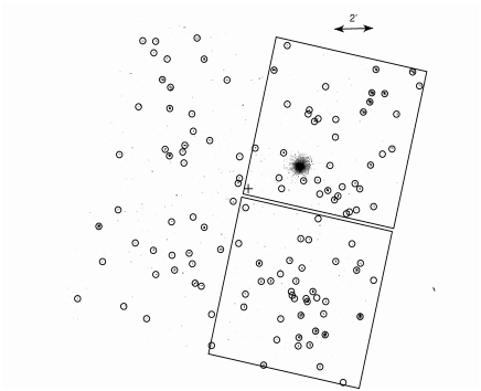
Figure 3: ($Top$) MS1137+6625 0.5-2 keV image, circles represent the detected sources, the cross indicates the aim-point. ($Bottom$) 0.5-2 keV chip-by-chip logN-logS of the MS1137+6625 field. Dashed line represents the 2$\sigma$ confidence level of the CDFS+HDFN logN-logS.

Table 2: Statistical properties of the overdensities

		Soft		Hard
Cluster	Chip	N∘	P	N∘	P
		of $\sigma$		of $\sigma$
		(1)	(2)	(3)	(4)
MS1137+6625	I1	2.47	1.35%	3.10	0.20%
	I3†	2.36	1.83%	2.57	1.02%
CLJ0848+4456	I2	2.25	2.44%	2.41	1.60%
RDCS0910+5422	I3†	2.20	2.78%	2.97	0.30%
	I2	2.03	4.24%	*	*
MS2053-0449	I0	*	*	2.66	0.78%
	I3†	2.23	2.57%	2.46	1.43%

(1) Significance of the excess in units of $\sigma$ (Soft).
(2) Probability of upward Poisson fluctuation of reference field distribution (Soft).
(3) Significance of the excess in units of $\sigma$ (Hard)
(4) Probability of upward Poisson fluctuation of reference field distribution(Hard).
^† Chip containing the cluster.

5.2 Cluster fields

Figure 4: logN-logS normalization vs. slope relations for overdense cluster fields in the soft ($Top\leavevmode\nobreak\ left\leavevmode\nobreak\ panel$) and hard band ($Bottom\leavevmode\nobreak\ left\leavevmode\nobreak\ panel$). The same relation in cluster fields with non-significant or no excesses in the soft ($Top\leavevmode\nobreak\ right\leavevmode\nobreak\ panel$) and hard band ($Bottom\leavevmode\nobreak\ right\leavevmode\nobreak\ panel$).

Figure 5: Distribution of the logN-logS normalizations in cluster and reference fields, in the soft ($Left\leavevmode\nobreak\ Panel$) and hard ($Right\leavevmode\nobreak\ Panel$) energy bands.

As an example we first show the results obtained in the field of MS 1137+6625. Fig. 3 ($Top$) clearly shows that the source density in the two boxed chips (one of which contains MS1137+6625) is about twice that in the other two chips. Chip-by-chip logN-logS have been calculated and are shown in Fig. 3. They are compared to the CDFS+HDFN logN-logS (CDFSN, $\pm 2\sigma$ deviations) that has a best fit set of parameters within 5% of the mean value given in Sect. 5.1. For two chips the logN-logS show a source surface density twice that in the CDFSN.

As detailed above (see Sect. 2 and Table 1), a similar analysis was performed on 10 cluster fields for a total of 40 chips, i.e. a sky coverage of $\sim 0.8$ deg². Best-fit normalizations and slopes for the logN-logS in the soft and hard energy bands are shown in Fig. 4, and compared to the average values of the reference fields (marked with diamonds in the figures). In six chip (from 4 cluster fields) excesses of a factor $\sim$1.7-2 with a significance $>2\sigma$ are detected. These are clearly seen in Fig. 4 ($Left\leavevmode\nobreak\ Panels$), and cluster-by-cluster statistics are given in Table 2. The excesses are located in the chip containing the cluster and in the adjoining chip. In the Lynx field (here named CL J0848+4456) the excess is observed in the only chip without a cluster (i.e. in this field three clusters were detected).

The other 6 fields (24 chips) do not show any significant ($>2\sigma$) excess. Nevertheless, in four out of these six cluster fields, given the low statistics, factor $\sim 2$ deviations cannot be statistically ruled out either. Altogether, we find at least 4 clusters out of 10 with significant overdensities on angular scales of $8\arcmin\times 8\arcmin$ or $8\arcmin\times 16\arcmin$.

It is worth noting that when calculated over the entire FOVs, these excesses are smoothed out and the logN-logS become statistically consistent with the reference fields on the same angular scales.

Fig. 5 shows the histograms of the normalization $k$ in cluster and reference fields (chip-by-chip). The histograms clearly show that the distributions have an almost Gaussian shape in the reference fields, both in the soft (Fig. 5, $Left$) and hard (Fig. 5, $Right$) energy bands. Instead, in the cluster fields, the distributions have a prominent tail at high values of k, containing about 20-25% of the fields. The significance of the tail can be quantified with a KS test which yields a probability that the two distributions are extracted from the same parent population of 9.03$\times 10^{-3}$ in the soft band and 2.55$\times 10^{-6}$ in the hard band.

5.3 Overdensities as a function of z

A very interesting result obtained from the present analysis is the apparent correlation found between the amplitude of the overdensities and the cluster redshifts, as shown in Fig. 6. In this figure, the the (2-10 keV) $k$ normalized to the value of the reference fields increases with the cluster redshift. The correlation is significant at a level of $\sim 96\%$ yielding a correlation parameter r=0.69 for 10 independent points. The best-fit linear relation is here R=(0.63$\pm$0.24)$z$+0.9$\pm$0.2 in the hard band while a similar relation R=(0.55$\pm 0.10$)$z$+1.06$\pm 0.16$ is obtained in the soft band.

Figure 6: Overdensities ($k_{\rm{clusters}}/k_{\rm{reference}}$) as a function of cluster redshift, in the hard band.

6 Discussion

The surface density of the X-ray serendipitous sources around 10 high $z$ clusters has been investigated with $Chandra$ and compared to the surface density of 5 reference cluster-free fields observed with similar exposure times. Four of the cluster fields show a factor $\sim$2 overdensity of sources at a $>$2$\sigma$ significance level, while there clearly are no similar deviations present in the reference fields.

The fact that, as shown in Fig. 5, a fraction of $\sim$25% of all fields near clusters shows overdensities demonstrates that this effect is unlikely to be associated to random statistical fluctuations constitutes a peculiar property of cluster fields. With the present work, the number of known high $z$ clusters showing such excesses increases to eleven. At a first glance, this contradicts what is reported in Kim et. al (2004) who find no significant difference between cluster and cluster-free fields (62 fields in total). Those authors, however, searched for source count differences on larger angular scales than in the present work. This may have had the effect of smoothing any excess signal. In support of the above argument we find that integrating our data over the whole (16$\arcmin$$\times$16$\arcmin$) ACIS-I FOVs, we find no statistically significant difference between fields either. In other words, this is consistent with an increase, in cluster fields, of the angular correlation signal toward lower angular scales (see e.g. D’Elia et al. 2004).

It should also be mentioned here that the present study yields one of the most sensitive measurements of the X-ray cosmic variance in empty fields available to date. Indeed, on scales of 8$\arcmin$$\times$8$\arcmin$ as reported in $Sect.5.1$ and clearly shown in Fig. 5, we find (1$\sigma$) fluctuations in number counts of the order of 17% and 13% in the soft and hard band, respectively. On scales 16$\arcmin$$\times$16$\arcmin$, these values decrease to 8% and 7% in the soft and hard band, respectively.

Considering that, if the detected X-ray sources are associated with the clusters themselves, their average luminosity must be of the order of $\sim$10^42-44 erg/s at $z$=0.5 and $\sim$10^43-44.5 erg/s at $z$=1.2, they are most likely to be active galactic nuclei. This is also supported by the power–law shape of their summed spectra (see Sect. 3). Moreover, if connected with the clusters, the angular scales on which the overdensities emerge correspond to linear distances of the order of 3-7 Mpc (at $z$=$0.5$ and $1.2$, respectively). This is somewhat greater than the typical dynamical radius of $<$3 Mpc for a massive cluster.

A number of explanations have been proposed in the literature (e.g. Cappi et al. 2001) to explain this kind of excess of X-ray sources, e.g.: gravitational lensing, triggering of AGN/starburst activity or filamentary clustering.

The hypothesis that some of the detected sources are magnified by gravitational lensing seems rather unlikely because i) the shapes of the logN-logS do not get steeper at fainter fluxes, as required by lensing in order to obtain a significant increase in the surface density of faint sources, and ii) the most distant clusters have $Einstein$ angles of the order $<1\arcmin$, much smaller than the angular scale of the excess. This further confirms previous findings by Cappi et al. (2001) and Johnson et al. (2003), based on the calculations done by Refregier & Loeb (1997).

Butcher & Oemler (1984) discovered that the fraction of blue (active) galaxies is very low ($<<$10%) in nearby clusters but increases linearly with the cluster redshift (percentages of several tens at $z$=0.5). This may well explain, at least qualitatively, the redshift-dependence found here in the X-ray band (Fig. 6). Simulations suggest that this effect could be caused by the interaction of the intra-cluster with the interstellar medium in those galaxies which are falling into the cluster potential well (see e.g Evrard et al. (1991)), thereby triggering AGN/Starburst activity. However, such an explanation faces the problem that the scales involved here ($>$3 Mpc) are substantially greater than typical virial radii, thus it is not clear how much diffuse gas would be available at those distances to trigger such an interaction.

The third hypothesis, that the excesses could represent filaments of the large-scale structure of the Universe, is in our opinion the most likely explanation. In the current vision of the Universe, clusters lie in the knots of a filamentary web-like network of galaxies and Dark Matter (see e.g. Peebles, 1993). This has been demonstrated by both hydrodynamic simulations (Bond et al. 1996,Colberg et al. 2000) and by extensive optical imaging and spectroscopic observations of galaxies around clusters (e.g. Gioia et al. 1999, Ebeling et al. 2004, Le Fèvre et al. 2004).

If AGNs trace galaxies (as observations clearly indicate, see for example Fig. 13 in Kauffmann et al, 2004), it is thus possible that we are observing AGNs in filaments connected with the clusters themselves. The detailed study by D’Elia et al. (2004) of the field surrounding the cluster 3C295 at $z$=0.5 clearly shows a strong and asymmetric clustering of X-ray sources on scales of a few arcmin. This dataset is, to our opinion, one of the best pieces of evidence to date for a filament at $z\sim$0.5 traced by X-ray emitting AGNs. Spectroscopic identification of the sources is being carried out and some redshifts close to that of the cluster give a first hint of a spatial connection between the overdensity and the cluster itself (D’Elia, private communication). Ohta et al. (2003) recently discovered in the optical band an overdensity of bright QSOs (a QSO-supercluster) and several groups of galaxies in the cluster field CL J0848+4456 at z$\sim 1.2$. This cluster field also shows an excess of X-ray sources (Fig. 4), and thus could be related to the large-scale structure at $z\sim$1.2. Unfortunately, these optically identified quasars are spread over an area (30$\arcmin$$\times$30$\arcmin$) much larger than the Chandra FOV (see Fig. 3 in Ohta et al. 2003). Therefore only four identifications (one QSO at $z\sim$1.26, one at $z\sim$0.88 and two at $z\sim$0.58) are in common making conclusions uncertain. Assuming that the excesses are indeed linked to the large scale structure of the Universe, the redshift-dependence of the overdensities (Fig. 6) could, in turn, be explained as a geometrical effect.

In order to firmly establish whether the X-ray overdensities found here are associated to large-scale structures at high $z$, extensive spectroscopic follow-up observations similar to those performed by e.g. Gioia et al. (1999), Ebeling et al. (2004), are required.

But clearly X-ray studies of source overdensities around high $z$ clusters might be a rather efficient way of mapping the cosmic web at high $z$.

7 Conclusions

The first systematic study of the serendipitous X-ray source density around high $z$ galaxy clusters has been performed with Chandra. For the first time the results of study have been compared to a sample of cluster-free fields which also allowed a detailed measurement of the cosmic variance. Forty percent of the cluster fields present strong statistically significant overdensities. The first, although not robust, evidence for a redshift dependence of these excesses has also been presented.

We speculate that filaments connected to the clusters are the most likely astrophysical interpretation of the above results. However, thought less likely, other effects such as an “X-ray Butcher Oemler effect” cannot be completely ruled out.

8 Acknowledgments

We wish to thank P. Mazzotta, A. Vikhlinin, I. Gioia and F. Fiore for many useful comments. N.C thanks R. Della Ceca who provided the logN-logS fitting package, Matteo Genghini, Enrico Franceschi and Fulvio Gianotti for software–related assistance. The entire $Chandra$ team, who made these observations possible, is acknowledged. Financial support from ASI and MIUR is kindly acknowledged.

References

- (1) Bond J. R., et al. , 1996, Nature, 380, 603
- (2) Brandt, W. N. et al. 2001, AJ, 122, 2810
- (3) Butcher, H. & Oemler, A. 1984, ApJ, 285, 426
- (4) Cappi, M. et al. 2001, ApJ, 548, 624
- Colberg et al. (2000) Colberg, J. M., White, S. D. M., MacFarland, T. J., Jenkins, A., Pearce, F. R., Frenk, C. S., Thomas, P. A., & Couchman, H. M. P. 2000, MNRAS, 313, 229
- (6) Crawford, D. F., Jauncey, D. L., & Murdoch, H. S. 1970, ApJ, 162, 405
- (7) D’Elia, V. et al., 2004, A&A in press, (astro-ph/0403401)
- Dressler, Thompson, & Shectman (1985) Dressler, A., Thompson, I. B., & Shectman, S. A. 1985, ApJ, 288, 481
- Dressler et al. (1999) Dressler, A., Smail, I., Poggianti, B. M., Butcher, H., Couch, W. J., Ellis, R. S., & Oemler, A. J. 1999, ApJS, 122, 51
- Ebeling, Barrett, & Donovan (2004) Ebeling, H., Barrett, E., & Donovan, D. 2004, ApJ, 609, L49
- (11) Eddington, A. S. 1940, MNRAS, 100, 354
- (12) Evrard, A. E. 1991, MNRAS, 248, 8P
- (13) Freeman et al., 2002, ApJ, 138, 185
- (14) Giacconi, R. et al. 2001, ApJ, 551, 624
- Gioia et al. (1990) Gioia, I. M., Maccacaro, T., Schild, R. E., Wolter, A., Stocke, J. T., Morris, S. L., & Henry, J. P. 1990, ApJS, 72, 567
- Gioia et al. (1999) Gioia, I. M., Henry, J. P., Mullis, C. R., Ebeling, H., & Wolter, A. 1999, AJ, 117, 2608
- Henry & Briel (1991) Henry, J. P. & Briel, U. G. 1991, A&A, 246, L14
- (18) Johnson, O., Best, P. N., & Almaini, O. 2003, MNRAS, 343, 924
- (19) Kaufmann, J. et al. 2004, submitted to MNRAS, astro-ph/0402030
- Kim et al. (2004) Kim, D.-W., et al. 2004, ApJ, 600, 59
- (21) Le Fèvre, O., et al. 2004, A&A, 417, 839
- Martini, Kelson, Mulchaey, & Trager (2002) Martini, P., Kelson, D. D., Mulchaey, J. S., & Trager, S. C. 2002, ApJ, 576, L109
- (23) Manners, J. C. 2002, Phd Thesis, Univ. Edimburgh
- (24) Molnar, S. M., Hughes, J. P., Donahue, M., & Joy, M. 2002, ApJ, 573, L91
- Moretti, Campana, Lazzati, & Tagliaferri (2003) Moretti, A., Campana, S., Lazzati, D., & Tagliaferri, G. 2003, ApJ, 588, 696
- (26) Murdoch, H. S., Crawford, D. F., & Jauncey, D. L. 1973, ApJ, 183, 1
- (27) Ohta, K. et al. 2003, ApJ, 598, 210
- (28) Peebles, J. E. 1993, Principles of Physical Cosmology (Princeton: Princeton Univ. Press)
- (29) Pentericci, L., Kurk, J. D., Röttgering, H. J. A., Miley, G. K., & Venemans, B. P. 2002, ASP Conf. Ser. 268: Tracing Cosmic Evolution with Galaxy Clusters, 27
- (30) Refregier, A. & Loeb, A. 1997, ApJ, 478, 476
- (31) Rosati, P. et al. 2002, ApJ, 566, 667
- (32) Schmitt, J. H. M. M. & Maccacaro, T. 1986, ApJ, 310, 334
- (33) Soltan et al. 2001, A&A, 378, 735
- (34) Stark, A. A., Gammie, C. F., Wilson, R. W., Bally, J., Linke, R. A., Heiles, C., & Hurwitz, M. 1992, ApJS, 79, 77
- (35) Stern, D. et al. 2002, AJ, 123, 2223
- (36) Tozzi, P. et al. 2001, ApJ, 562, 42
- (37) Vikhlinin, A. & Forman, W. 1995, ApJ, 455, L109
- Yang et al. (2003) Yang, Y., Mushotzky, R. F., Barger, A. J., Cowie, L. L., Sanders, D. B., & Steffen, A. T. 2003, ApJ, 585, L85
- (39) Wang, J. X. et al. 2004, AJ, 127, 213