Time evolution of the stochastic linear bias of interacting galaxies on linear scales

We extend the time dependent bias model of Tegmark & Peebles (1998) to predict the large-scale evolution of the stochastic linear bias of different galaxy populations with respect to both the dark matter and each other. The resulting model equations contain a general expression, coined the “interaction term”, accounting for the destruction or production of galaxies. This term may be used to model couplings between different populations that lead to an increase or decrease of the number of a galaxies belonging to a population, e.g. passive evolution or merging processes. This is explored in detail using a toy model. In particular, it is shown that the presence of such a coupling may change the evolution of the bias parameter compared to an interaction-free evolution. We argue that the observation of the evolution of the large-scale bias and galaxy number density with wide-field surveys may be used to infer fundamental interaction parameters between galaxy populations, possibly giving an insight in their formation and evolution.

1 Introduction

The first studies of large scale structure had to completely rely on galaxies as mass tracers of the large scale Universe. It became clear that in order to match the clustering statistics of galaxies with models for gravitationally driven structure formation - in particular with the SCDM favoured in the early 90s - galaxies cannot be perfect tracers of the overall mass density field; the concept of galaxy biasing was born (e.g. Bardeen et al. 1986, BBKS hereafter; Davis et al. 1985).

The first bias description was introduced by Kaiser (1984) as a single parameter that rescales the two-point correlation function (2PCF) of the galaxy density field to yield the expected 2PCF for matter clustering. Such a rescaling can be achieved if the fluctuation field or density contrast $\delta_{\rm m}\equiv\rho_{\rm m}/\bar{\rho}_{\rm m}-1$ of the matter density field is a linear function of the galaxy density contrast $\delta_{\rm g}\equiv{\rm n}_{\rm g}/\bar{\rm n}_{\rm g}-1$, thus $\delta_{\rm b}=b\delta_{\rm m}$. $\rho_{\rm m}$ and ${\rm n}_{\rm g}$ are the matter and galaxy number density fields respectively. The bar denotes the mean density. A possible reason for the enhancement of clustering could be that galaxies are preferentially formed in the peaks of the dark matter field (Kaiser 1984; BBKS).

This linear biasing scheme was put in a more general framework by Fry & Gaztańaga (1993) who proposed $\delta_{\rm g}$ to be an arbitrary analytic local function of $\delta_{\rm m}$ (local Eulerian biasing), opening the door to (in principal arbitrarily many) bias parameters which, however, can be measured if higher-order statistics is invoked. Moreover, these parameters can be different if different smoothing scales of the density fields are considered (scale-dependence of bias). An alternative picture to the Eulerian model is to assume that the galaxy distribution or a part of it (like recently formed galaxies) is only a local function of the dark matter field at one particular time (Lagrangian bias: e.g. Catelan et al. 2000).

In order to look at general features of the statistics of transformed random fields, Coles (1993) derived constraints for the clustering of galaxies that follow from a local mapping of a Gaussian field. It was found that on large scales where clustering is small - even for a non-local mapping that, however, preserves the clustering hierarchy (Coles, Melott & Munshi 1999; Scherrer & Weinberg 1998) - the shape of the 2PCF of the matter and the galaxies is identical, so that here a simple linear bias scheme may still be used (see also Narayanan, Berlind & Weinberg 2000 and Mann, Peacock & Heavens 1998).

Another degree of freedom had to be inserted into the biasing schemes, once it was realised that the relation between the matter and the galaxy density field is very likely to be a stochastic one (Blanton 2000; Tegmark & Bromley 1999; Dekel & Lahav 1999; Matsubara 1999; Cen & Ostriker 1992) due to “hidden parameters” of galaxy formation/evolution that cannot be incorporated into a simple picture that involves only the densities. Currently, the description for stochastic nonlinear biasing most commonly used is by Dekel & Lahav (1999). It expresses the joint probability distribution $P\left(\delta_{\rm g},\delta_{\rm m}\right)$ of local values for $\delta_{\rm g}$ and $\delta_{\rm m}$ in terms of the conditional mean $\big{\langle}\delta_{\rm g}|\delta_{\rm m}\big{\rangle}$ and the scatter $\delta_{\rm g}-\big{\langle}\delta_{\rm g}|\delta_{\rm m}\big{\rangle}$ about the conditional mean. For $P\left(\delta_{\rm g},\delta_{\rm m}\right)$ being a bivariate Gaussian this scheme reduces to the following stochastic linear biasing parameters

$$b\equiv\sqrt{\frac{\big{\langle}\delta^{2}_{\rm g}\big{\rangle}}{\big{\langle}\delta^{2}_{\rm m}\big{\rangle}}}\;\;;\;\;r\equiv\frac{\big{\langle}\delta_{\rm m}\delta_{\rm g}\big{\rangle}}{\sqrt{\big{\langle}\delta^{2}_{\rm g}\big{\rangle}\big{\langle}\delta^{2}_{\rm m}\big{\rangle}}}\;,$$ (1)

which is approximately fulfilled on large scales. Equivalently, one can express the bias parameters in terms of auto- and cross-correlation power spectra $P_{\rm m}=\big{\langle}\tilde{\delta}_{\rm m}\tilde{\delta}_{\rm m}^{\ast}\big{\rangle}^{\prime}$, $P_{\rm gg}=\big{\langle}\tilde{\delta}_{\rm g}\tilde{\delta}_{\rm g}^{\ast}\big{\rangle}^{\prime}$ and $P_{gm}=\big{\langle}\tilde{\delta}_{\rm m}\tilde{\delta}_{\rm g}^{\ast}\big{\rangle}^{\prime}$:

$$b\left(k\right)\equiv\sqrt{\frac{P_{\rm gg}\left(k\right)}{P_{\rm m}\left(k\right)}}\;\;\;\;r\left(k\right)\equiv\frac{P_{\rm gm}\left(k\right)}{\sqrt{P_{\rm gg}\left(k\right)P_{\rm m}\left(k\right)}}\;,$$ (2)

where $\tilde{\delta}_{\rm g}$ and $\tilde{\delta}_{\rm m}$ are the Fourier transforms of the density contrasts. The asterisk “$\ast$” denotes the complex conjugate. For the Fourier space definition above, the relevant scale for the bias parameters is defined by the spatial frequency considered, whereas in the other definition a scale is defined by smoothing the fields with a kernel of a certain size. In the case of a strict positive correlation $r=1$, the prescription reduces to the former deterministic linear bias with only one free parameter $b$.

Nowadays, in a time of a “concordance” cosmological model (Spergel et al. 2003), cosmic microwave background and weak gravitational lensing studies provide information on the matter distribution almost independent of the galaxy distribution, confirming the original paradigm of structure formation, in particular the $\Lambda$CDM model. Conversely, this also confirms the early suspicion that galaxies are not perfect mass tracers. Intriguingly, in contrast to about ten years ago when SCDM was the favoured cosmological model, with $\Lambda$CDM almost no bias in the local Universe on large scales is required (Verde et al. 2002). However, there is a need for bias on smaller scales (scale-dependent bias), because in contrast to that of the dark matter the 2PCF of the galaxies is a power law over several orders of magnitude. The exact scale-dependence of the bias maybe even hold some information on the physics of galaxy formation (e.g. Benson et al. 2000; Blanton et al. 1999).

The evolution of bias has also become a matter of interest: there is evidence that galaxy clustering is a function of redshift (e.g. Carlberg et al. 2000; Adelberger et al. 1998; Le Fevre et al. 1996) and even that the galaxy bias is a decreasing function of redshift (e.g. Blanton et al. 2000; Magliocchetti et al. 2000; Steidel et al. 1998; Wechsler et al. 1998; Matarrese et al. 1997).

Analytical models for the bias evolution fall into two categories: test particle models and halo models. Test particle models (Basilakos & Plionis 2001; Matsubara 1999; Taruya & Soda 1999; Taruya et al. 1999; Tegmark & Peebles 1998, hereafter TP98; Fry 1996, hereafter F96; Nusser & Davis 1994) assume that galaxies passively follow the bulk flow of the dark matter field which then can be treated with conventional perturbation theory. Halo models (Seljak 2000; Peacock & Smith 2000; Sheth & Lemson 1999; Bagla 1998; Catelan et al. 1998; Mo & White 1996), on the other hand, picture the dark matter density field to be made up out of typical haloes that host galaxies, so that the clustering of galaxies is related to the clustering of their hosts and typical halo properties. Both concepts agree on a debiasing of the galaxy field with time, but there are differences in the details (Magliocchetti et al. 2000).

If one does not look at the galaxy population as a whole, which as noted above seems to trace the local matter distribution quite well on large scales, there are more interesting features. It is also known that different types of galaxies are differently clustered with respect to each other, and, consequently, also with respect to the underlying dark matter field (e.g. Phleps & Meisenheimer 2003 and references therein; Norberg et al. 2002; Blanton et al. 2000). At low redshift, the correlation length - a measure for the strength of clustering - is a function of morphological type and color (Tucker et al. 1997; Loveday et al. 1995; Davis & Geller 1976) and maybe also depend on the luminosity of the galaxy population (Benoist et al. 1996). Furthermore, there are examples of galaxy populations whose relative clustering is known to have changed with time. For instance, red and blue galaxies were almost not biased with respect to each other at $z\geq 0.5$ (Le Fevre et al. 1996; but also see Phleps & Meisenheimer 2003 who do not observe this bias), but today early type galaxies are more strongly clustered than late types (e.g. Norberg 2002; Baker et al. 1998).

Thus, it makes sense to conceive a model for bias evolution that takes into account several distinct galaxy populations.

Observationally, the stochastic linear bias can be measured by redshift space distortions (Sigad, Branchini & Dekel 2000; Pen 1998; Kaiser 1987), weak gravitational lensing (Fan 2003; Hoekstra et al. 2002; van Waerbeke 1998; Schneider 1998) and counts-in-cells statistics (Conway et al. 2004; Tegmark & Bromley 1999; Efstathiou et al. 1990); the latter, however, only for biasing between galaxies. Future surveys with an appropriate number of galaxies will be required to obtain a good signal-to-noise ratio for reconstruction of the evolution of bias.

In this paper, we extend the test particle model of TP98 for the stochastic linear parameter evolution and include several galaxy populations that are allowed to interact with each other. The rate of galaxy interaction is assumed to be a function of all density fields, changing in general the number of members of a particular galaxy population. Treated is also the evolution of the relative bias of the populations with respect to each other, not only the bias relative to the dark matter field.

In detail, the second section develops a model based on the bulk flow hypothesis including a general sink/source term for galaxies. We derive differential equations for the auto- and cross-correlation power spectra (galaxy-galaxy, galaxy-dark matter), valid on scales where the fields are Gaussian, thus on linear scales (Sect. 2.3). The equations are then transformed to obtain differential equations for the stochastic linear bias parameters (Sect. 2.4). In Sect. 3, we focus on linear and quadratic interaction rates and work out the relevant terms needed for the bias model equations based on this interaction (table 1). We demonstrate in Sect. 4 for a few toy models the effect on the evolution of the large scale bias in the presence of galaxy interactions. We conclude this paper with a discussion.

2 Derivation of the bias model

2.1 Evolution of density contrasts

Here we derive differential equations for the density contrasts of a set of galaxy species that are assumed to be perfect velocity tracers, meaning that their bulk velocities are identical to the overall bulk mass flow.

It is common practice to express the density fields - dark matter $\rho_{\rm m}$ and galaxies $n_{i}$, $i=1..N$ - in terms of the their mean density and the fluctuation about this mean, the density contrast:

$$\rho_{\rm m}=\bar{\rho}_{\rm m}\left(1+\delta_{\rm m}\right) n_{i}=\bar{n}_{i}\left(1+\delta_{i}\right)\;.$$ (3)

$\bar{\rho}_{\rm m}\equiv\langle\rho_{\rm m}\rangle$ and $\bar{n}_{i}\equiv\langle n_{i}\rangle$ are the corresponding matter and number density respectively, obtained by taking the volume average. Under the usual hydrodynamic conditions and cosmological assumptions (Peebles 1980), the gravitationally driven evolution of the dark matter density and bulk flow ${\bf v}$ (deviation from the Hubble flow) is described in comoving coordinates by

$$\frac{\partial\theta}{\partial t}+\left(1-\frac{\Omega_{\rm m}}{2}+\Omega_{\Lambda}\right)H\left(a\right)\theta$$

$$+\frac{3}{2}H\left(a\right)\Omega_{\rm m}\delta_{\rm m}+\frac{1}{a^{2}H\left(a\right)}\nabla\left({\bf v}\nabla\right){\bf v} = 0$$ (4)

$$\frac{\partial\delta_{\rm m}}{\partial t}+H\left(a\right)\theta+\frac{1}{a}\nabla\left(\delta_{\rm m}{\bf v}\right) = 0$$ (5)

$$H\left(a\right)=H_{0}\sqrt{\Omega_{\rm m}a^{-3}+\left(1-\Omega_{\rm m}-\Omega_{\Lambda}\right)a^{-2}+\Omega_{\Lambda}}\;.$$ (6)

$\theta\equiv\nabla{\bf v}/\left[aH\left(a\right)\right]$ is related to the curl free component of the bulk flow. On large scales, this is the only component (in contrast to the vorticity) that is not suppressed by structure growth and therefore the only one relevant for structure formation. $H\left(a\right)\equiv\dot{a}/a$ is the Hubble parameter. Solutions to Eqs. (4)-(6) have been extensively studied in the literature, especially using the perturbation approach (e.g. Bernardeau et al. 2001 for a review; Goroff et al. 1986) and therefore will not be discussed here. We simply assume that the solutions for $\delta_{\rm m}$ and ${\bf v}$ or $\theta$ are (approximately) known.

The central assumption in this and similar models (e.g. TP98; F96) is that the velocity fields of the galaxies are identical to that of the dark matter. One thereby reduces the treatment for the galaxy number density solely to the number conservation equation, which for a conserved number of galaxies looks as Eq. (5) (TP98):

$$\frac{\partial\delta_{i}}{\partial t}+H\left(a\right)\theta+\frac{1}{a}\nabla\left(\delta_{i}{\bf v}\right)=0\;.$$ (7)

The term $H\left(a\right)\theta$ can be removed by subtracting Eq. (5), arriving at an equation that clearly shows how the galaxies are coupled to the dark matter field

$$\frac{\partial\delta_{i}}{\partial t}=\frac{\partial\delta_{\rm m}}{\partial t}+\frac{1}{a}\nabla\left({\bf v}\left[\delta_{\rm m}-\delta_{i}\right]\right)\;.$$ (8)

Our main modification consists of dropping the constraint that the mean number of galaxies - expressed by $\bar{n}_{i}$ - is conserved. We allow for a sink/source term $\Phi_{i}$ in the mass conservation equation for the galaxy population $n_{i}$ that incorporates galaxy-galaxy and galaxy-dark matter interactions, and is thought to be a function of all the density fields. Note that in this formalism interaction is equivalent to a change in galaxy number density.

In order to include $\Phi_{i}$ in Eq. (7) and to eventually obtain a modified formula (8), we have to start with the number conservation equation for the galaxies plus the new interaction rate $\Phi_{i}$:

$$\frac{\partial n_{i}}{\partial t}+\frac{1}{a}\nabla\left({\bf v}n_{i}\right)=\Phi_{i}\;.$$ (9)

Setting $\Phi_{i}=0$ would result again in Eq. (8). Substitution of $n_{i}$ by the definition in (3) yields:

$$\frac{\partial\delta_{i}}{\partial t}+H\left(a\right)\theta+\frac{1}{a}\nabla\left({\bf v}\delta_{i}\right)=\frac{1}{\bar{n}_{i}}\left[\Phi_{i}-\left(1+\delta_{i}\right)\frac{\partial\bar{n}_{i}}{\partial t}\right]\;.$$ (10)

For the last step we had to take into account that the mean galaxy density $\bar{n}_{i}$ is a function of time. Compared to Eq. (7), we obviously have a new term on the right hand side (rhs) that has to be cared for. Again, subtracting Eq. (5) from the last equation gives the time evolution equation for the density contrasts of the galaxies but this time accounting for the impact of a varying mean galaxy density due to $\Phi_{i}$

$$\frac{\partial\delta_{i}}{\partial t}=$$ (11)

$$\frac{\partial\delta_{\rm m}}{\partial t}+\frac{1}{a}\nabla\left({\bf v}\left[\delta_{\rm m}-\delta_{i}\right]\right)+\frac{1}{\bar{n}_{i}}\left[\Phi_{i}-\delta_{i}\frac{\partial\bar{n}_{i}}{\partial t}\right]-\frac{1}{\bar{n}_{i}}\frac{\partial\bar{n}_{i}}{\partial t}\;.$$

2.2 Evolution of mean densities

In order to get the time-dependence of the mean galaxy density $\bar{n}_{i}$, we take the ensemble average $\big{\langle}...\big{\rangle}$ of Eq. (11):

$$\frac{\partial\bar{n}_{i}}{\partial t}=\big{\langle}\Phi_{i}\big{\rangle}\;,$$ (12)

where we used $\big{\langle}\delta_{i}\big{\rangle}=\big{\langle}\delta_{m}\big{\rangle}=\big{\langle}\nabla\left({\bf v}\delta_{i}\right)\big{\rangle}=\nabla\big{\langle}{\bf v}\delta_{i}\big{\rangle}=0$.

The terms $\nabla\big{\langle}{\bf v}\delta_{\rm m}\big{\rangle}$ and $\nabla\big{\langle}{\bf v}\delta_{i}\big{\rangle}$ vanish, because the net flux

$$\big{\langle}\rho{\bf v}\big{\rangle}=\bar{\rho}\big{\langle}{\bf v}\delta\big{\rangle}+\bar{\rho}\big{\langle}{\bf v}\big{\rangle}=0$$ (13)

of any species $\rho$ over the whole volume has to be zero, since we work in the rest frame of the Hubble expansion. In particular, Eq. (12) has general validity and is not restricted to Gaussian fields only.

2.3 Linear scale evolution of correlation power spectra

We will primarily be interested in the evolution of the linear stochastic bias which may be expressed in terms of the cross- and auto-correlation power spectra. Therefore, the next logical step is to work out the time dependence of these power spectra. For that reason, we take the Fourier transform

$$\tilde{\delta}\left({\bf k}\right)=\frac{1}{\left(2\pi\right)^{3}}\int d^{3}{\bf r}\leavevmode\nobreak\ \delta\left({\bf r}\right){\rm e}^{-{\rm i}{\bf k}{\bf r}}$$ (14)

of Eq. (11) to obtain the corresponding equation for the Fourier coefficients

$$\frac{\partial\tilde{\delta}_{i}}{\partial t}=$$ (15)

$$\frac{\partial\tilde{\delta}_{\rm m}}{\partial t}+\frac{1}{\bar{n}_{i}}\left[\tilde{\Phi}_{i}-\tilde{\delta}_{i}\frac{\partial\bar{n}_{i}}{\partial t}\right]+\frac{\rm i\leavevmode\nobreak\ {\bf k}}{a}\left({\bf\tilde{v}}\ast\left[\tilde{\delta}_{\rm m}-\tilde{\delta}_{i}\right]\right)\;,$$

where the irrelevant terms at ${\bf k}=0$ have been neglected. For convenience, we omit the arguments in the brackets of the Fourier coefficients. By the asterisk “$\ast$” we denote the convolution of two fields in Fourier space

$$\left(\tilde{f}\ast\tilde{g}\right)\left({\bf k}\right)\equiv\frac{1}{\left(2\pi\right)^{3}}\int d^{3}{\bf k}^{\prime}\tilde{f}\left({\bf k}^{\prime}\right)\tilde{g}\left({\bf k}-{\bf k}^{\prime}\right)$$ (16)

that enter when products of fields are Fourier transformed. A tilde “$\leavevmode\nobreak\ \tilde{}\leavevmode\nobreak\$” always denotes the Fourier transform of a random field or function beneath the tilde.

We restrict ourselves to the case of strictly Gaussian fields, which is a reasonable assumption on linear scales (see e.g. Bernardeau et al. 2002). As a consequence, all connected higher order correlation terms like bispectra vanish, which makes the following equations a lot simpler. Further, in the cosmological context the density fields are isotropic and homogeneous random fields.

The correlation power spectrum $P\left({\bf k}\right)$ between two homogeneous random field with the Fourier coefficients $\tilde{\delta}_{1}\left({\bf k}\right)$ and $\tilde{\delta}_{2}\left({\bf k}\right)$ respectively is

$$\left(2\pi\right)^{3}\delta_{D}\left({\bf k}-{\bf k}^{\prime}\right)P\left({\bf k}\right)\equiv\big{\langle}\tilde{\delta}_{1}\left({\bf k}\right)\tilde{\delta}_{2}^{\ast}\left({\bf k}^{\prime}\right)\big{\rangle}\;,$$ (17)

stating that homogeneity requires only the Fourier coefficients of the same ${\bf k}$ to be correlated. This relation also states that the power spectrum $P\left({\bf k}\right)$ is related to the correlator in the following way

$$P\left({\bf k}\right)=\int\frac{d^{3}{\bf k}^{\prime}}{\left(2\pi\right)^{3}}\big{\langle}\tilde{\delta}_{1}\left({\bf k}\right)\tilde{\delta}_{2}^{\ast}\left({\bf k}^{\prime}\right)\big{\rangle}\;.$$ (18)

Due to this relation, we are going to use a slightly different definition $\big{\langle}...\big{\rangle}^{\prime}$ of the ensemble average:

$$\Big{\langle}\tilde{\delta}_{1}\left({\bf k}\right)\tilde{\delta}_{2}^{\ast}\left({\bf k}^{\prime}\right)\Big{\rangle}^{\prime}\equiv\int\frac{d^{3}{\bf k}^{\prime}}{\left(2\pi\right)^{3}}\big{\langle}\tilde{\delta}_{1}\left({\bf k}\right)\tilde{\delta}_{2}^{\ast}\left({\bf k}^{\prime}\right)\big{\rangle}\;,$$ (19)

which in the following is useful to derive the differential equations for the correlation power spectra. We also introduce the convention to omit the ${\bf k}$ arguments for the correlators and the power spectra. Instead, we use the following notation: Power spectra have as well as the first field in the two-point correlator (in the above definition $\tilde{\delta}_{1}$) as argument always ${\bf k}$, whereas the second field in the correlator has the argument ${\bf k}^{\prime}$. For example, according to this convention the following two lines are identical:

$$P\left({\bf k}\right) = \Big{\langle}\tilde{\delta}_{1}\left({\bf k}\right)\tilde{\delta}_{2}\left({\bf k}^{\prime}\right)^{\ast}\Big{\rangle}^{\prime}$$ (20)

$$P = \Big{\langle}\tilde{\delta}_{1}\tilde{\delta}_{2}^{\ast}\Big{\rangle}^{\prime}\;.$$

After explaining the notation, we now accordingly define the correlation power spectra between the model random fields by

$$P_{ij}=P_{ji}\equiv\Big{\langle}\tilde{\delta}_{i}\tilde{\delta}_{j}^{\ast}\Big{\rangle}^{\prime}\;\;\;\;P_{i}\equiv\Big{\langle}\tilde{\delta}_{i}\tilde{\delta}_{\rm m}^{\ast}\Big{\rangle}^{\prime}\;\;\;\;P_{\rm m}\equiv\Big{\langle}\tilde{\delta}_{\rm m}\tilde{\delta}_{\rm m}^{\ast}\Big{\rangle}^{\prime}\;,$$ (21)

where $P_{ij}$ is the correlation power spectrum between galaxy population $n_{i}$ and $n_{j}$, thus for $i=j$ the auto-correlation of population $n_{i}$. $P_{i}$ denotes the cross-correlation between the population $n_{i}$ and the dark matter field $\rho_{\rm m}$. $P_{\rm m}$ is the dark matter auto-correlation.

To work out their evolution, we first multiply both sides of Eq. (15) by $\tilde{\delta}_{\rm m}^{\ast}\left({\bf k}^{\prime}\right)$, take the (modified) ensemble average $\big{\langle}...\big{\rangle}^{\prime}$ and use the definition of the power spectra to get

$$\Big{\langle}\frac{\partial\tilde{\delta}_{i}}{\partial t}\tilde{\delta}_{\rm m}^{\ast}\Big{\rangle}^{\prime} = \Big{\langle}\frac{\partial\tilde{\delta}_{\rm m}}{\partial t}\tilde{\delta}_{\rm m}^{\ast}\Big{\rangle}^{\prime}+\frac{1}{\bar{n}_{i}}\left[\Big{\langle}\tilde{\Phi}_{i}\tilde{\delta}_{\rm m}^{\ast}\Big{\rangle}^{\prime}-P_{i}\frac{\partial\bar{n}_{i}}{\partial t}\right]\;.$$ (22)

Note that all terms containing bispectra (three-point correlations) have been neglected. They turn up when the correlation of two convolved fields with a third other field is calculated (see Appendix A) as for the velocity term in Eq. (15).

The equation simplifies further, if we use the following two relations, obtained by taking the time derivative of the power spectra definitions (21)

$$\frac{\partial P_{\rm m}}{\partial t} = \Big{\langle}\frac{\partial\tilde{\delta}_{\rm m}}{\partial t}\tilde{\delta}_{\rm m}^{\ast}\Big{\rangle}^{\prime}+\Big{\langle}\tilde{\delta}_{\rm m}\frac{\partial\tilde{\delta}_{\rm m}^{\ast}}{\partial t}\Big{\rangle}^{\prime}=2\Big{\langle}\frac{\partial\tilde{\delta}_{\rm m}}{\partial t}\tilde{\delta}_{\rm m}^{\ast}\Big{\rangle}^{\prime}$$ (23)

$$\Big{\langle}\frac{\partial{\tilde{\delta}}_{i}}{\partial t}\tilde{\delta}_{\rm m}^{\ast}\Big{\rangle}^{\prime} = \frac{\partial P_{i}}{\partial t}-\Big{\langle}\frac{\partial{\tilde{\delta}}_{\rm m}^{\ast}}{\partial t}\tilde{\delta}_{i}\Big{\rangle}^{\prime}\;.$$ (24)

Eq. (23) utilises the fact that the power spectra are real number functions, thus identical to its complex conjugate. Eq. (22) can according to Eq. (23) and (24) be written as

$$\frac{\partial P_{i}}{\partial t}=$$ (25)

$$\frac{1}{2}\frac{\partial P_{\rm m}}{\partial t}+\frac{1}{\bar{n}_{i}}\left[\Big{\langle}\tilde{\Phi}_{i}\tilde{\delta}_{\rm m}^{\ast}\Big{\rangle}^{\prime}-P_{i}\frac{\partial\bar{n}_{i}}{\partial t}\right]+\Big{\langle}\frac{\partial{\tilde{\delta}}_{\rm m}^{\ast}}{\partial t}\tilde{\delta}_{i}\Big{\rangle}^{\prime}$$

leaving us with an equation for the dark matter-galaxy power spectrum.

As a second step, we try to do a similar thing for the galaxy-galaxy power spectra $P_{ij}$. Multiplying both sides of (15) by $\tilde{\delta}_{j}^{\ast}\left({\bf k}^{\prime}\right)$ and taking the ensemble average yields:

$$\Big{\langle}\frac{\partial\tilde{\delta}_{i}}{\partial t}\tilde{\delta}_{j}^{\ast}\Big{\rangle}^{\prime} = \Big{\langle}\frac{\partial\tilde{\delta}_{\rm m}}{\partial t}\tilde{\delta}_{j}^{\ast}\Big{\rangle}^{\prime}+\frac{1}{\bar{n}_{i}}\left[\Big{\langle}\tilde{\Phi}_{i}\tilde{\delta}_{j}^{\ast}\Big{\rangle}^{\prime}-P_{ij}\frac{\partial\bar{n}_{i}}{\partial t}\right]\;.$$ (26)

This is already the first term out of two we need for the time evolution of $P_{ij}$:

$$\frac{\partial P_{ij}}{\partial t}=\Big{\langle}\frac{\partial\tilde{\delta}_{i}^{\ast}}{\partial t}\tilde{\delta}_{j}\Big{\rangle}^{\prime}+\Big{\langle}\frac{\partial\tilde{\delta}_{j}}{\partial t}\tilde{\delta}_{i}^{\ast}\Big{\rangle}^{\prime}\;.$$ (27)

The second is obtained by swapping the indices $i$ and $j$ and taking the complex conjugate of Eqs. (26). Combining these eventually gives

$$\frac{\partial P_{ij}}{\partial t} = \Big{\langle}\frac{\partial\tilde{\delta}_{\rm m}}{\partial t}\tilde{\delta}_{j}^{\ast}\Big{\rangle}^{\prime}+\frac{1}{\bar{n}_{i}}\left[\Big{\langle}\tilde{\Phi}_{i}\tilde{\delta}_{j}^{\ast}\Big{\rangle}^{\prime}-P_{ij}\frac{\partial\bar{n}_{i}}{\partial t}\right]$$

$$+ \Big{\langle}\frac{\partial\tilde{\delta}_{\rm m}^{\ast}}{\partial t}\tilde{\delta}_{i}\Big{\rangle}^{\prime}+\frac{1}{\bar{n}_{j}}\left[\Big{\langle}\tilde{\Phi}_{j}^{\ast}\tilde{\delta}_{i}\Big{\rangle}^{\prime}-P_{ij}\frac{\partial\bar{n}_{j}}{\partial t}\right]\;.$$

For the next step, we would like to approximate in Eqs. (25) and (2.3) the time derivative $\frac{\partial\tilde{\delta}_{\rm m}}{\partial t}$ using perturbation theory. For our purposes, the lowest order approximation of $\tilde{\delta}_{\rm m}$ is sufficient, because we have restricted the model to large (linear) scales where the cosmological fields may be considered as Gaussian random fields. Considering only the growing mode, to lowest order the density field of the dark matter $\tilde{\delta}_{\rm m}|_{t_{i}}$ is from one initial time $t_{i}$ onwards growing linearly, ${\bf k}$-independently with time (e.g. Bernardeau et al. 2002)

$$\tilde{\delta}_{\rm m} = D_{+}\leavevmode\nobreak\ \tilde{\delta}_{\rm m}|_{t_{i}}$$

$$\frac{\partial\tilde{\delta}_{\rm m}}{\partial t} = \frac{\partial D_{+}}{\partial t}\leavevmode\nobreak\ \tilde{\delta}_{\rm m}|_{t_{i}}=\frac{1}{D_{+}}\frac{\partial D_{+}}{\partial t}\leavevmode\nobreak\ \tilde{\delta}_{\rm m}=\frac{\partial\ln{D_{+}}}{\partial t}\leavevmode\nobreak\ \tilde{\delta}_{\rm m}$$ (29)

where $D_{+}$ can be shown to be the integral (e.g. Peacock 1999)

$$D_{+}\left(a\right)\propto H\left(a\right)\int_{0}^{a}da^{\prime}\frac{1}{\left[a^{\prime}H\left(a^{\prime}\right)\right]^{3}}\;.$$ (30)

A very good approximation to this integral is given by fitting formula of Carroll et al. (1992).

Employing the lowest order approximation of $\tilde{\delta}_{\rm m}$ yields for the terms in question

$$\Big{\langle}\frac{\partial\tilde{\delta}_{\rm m}^{\ast}}{\partial t}\tilde{\delta}_{i}\Big{\rangle}^{\prime} = \Big{\langle}\frac{\partial\ln{D_{+}}}{\partial t}\tilde{\delta}_{\rm m}^{\ast}\tilde{\delta}_{i}\Big{\rangle}^{\prime}=\frac{\partial\ln{D_{+}}}{\partial t}\leavevmode\nobreak\ P_{i}\equiv\frac{R\left(t\right)}{2}\leavevmode\nobreak\ P_{i}$$

$$\frac{\partial P_{\rm m}}{\partial t} = \Big{\langle}\frac{\partial\ln{D_{+}}}{\partial t}\tilde{\delta}_{\rm m}^{\ast}\tilde{\delta}_{\rm m}\Big{\rangle}^{\prime}+\Big{\langle}\tilde{\delta}_{\rm m}^{\ast}\frac{\partial\ln{D_{+}}}{\partial t}\tilde{\delta}_{\rm m}\Big{\rangle}^{\prime}$$ (31)

$$= 2\frac{\partial\ln{D_{+}}}{\partial t}\leavevmode\nobreak\ P_{\rm m}\equiv R\left(t\right)\leavevmode\nobreak\ P_{\rm m}\;.$$

The newly introduced function

$$R\left(t\right)\equiv\frac{1}{P_{\rm m}}\frac{\partial P_{\rm m}}{\partial t}=2\frac{\partial\ln{D_{+}}}{\partial t}$$ (32)

is the rate at which the power spectrum of the dark matter is growing on linear scales.

Plugging this expression into Eqs. (25) and (2.3) enables us to write the differential equations for the correlation power spectra in a closed form

$$\frac{\partial P_{i}}{\partial t}-R\left(t\right)\frac{P_{\rm m}+P_{i}}{2} = \frac{\Big{\langle}\tilde{\Phi}_{i}\tilde{\delta}_{\rm m}^{\ast}\Big{\rangle}^{\prime}}{\bar{n}_{i}}-P_{i}\frac{\big{\langle}\Phi_{i}\big{\rangle}}{\bar{n}_{i}}$$ (33)

$$\frac{\partial P_{ij}}{\partial t}-R\left(t\right)\frac{P_{j}+P_{i}}{2} = \frac{\Big{\langle}\tilde{\Phi}_{i}\tilde{\delta}_{j}^{\ast}\Big{\rangle}^{\prime}}{\bar{n}_{i}}+\frac{\Big{\langle}\tilde{\Phi}_{j}^{\ast}\tilde{\delta}_{i}\Big{\rangle}^{\prime}}{\bar{n}_{j}}$$

$$- P_{ij}\left[\frac{\big{\langle}\Phi_{i}\big{\rangle}}{\bar{n}_{i}}+\frac{\big{\langle}\Phi_{j}\big{\rangle}}{\bar{n}_{j}}\right]\;.$$

The terms on the left hand side (lhs) containing $R\left(t\right)$ are responsible for driving a biased galaxy distribution towards the dark matter distribution. Setting these terms to zero, switches off the coupling to the dark matter field due to the bulk flow assumption.

2.4 Linear scale evolution of stochastic linear bias

We define the bias parameters with one index, thus $r_{i}$ and $b_{i}$, to be the bias of the $i$th galaxy population with respect to the dark matter, whereas two indices, $b_{ij}$ and $r_{ij}$, denote the bias between the $i$th and $j$th galaxy population:

$$b_{i}\equiv\sqrt{\frac{P_{ii}}{P_{\rm m}}} r_{i}\equiv\frac{P_{i}}{\sqrt{P_{ii}P_{\rm m}}}$$ (35)

$$b_{ij}\equiv\sqrt{\frac{P_{ii}}{P_{jj}}} r_{ij}\equiv\frac{P_{ij}}{\sqrt{P_{ii}P_{jj}}}\;.$$

Using this definition, we can write down differential equations for $\left(b_{i}\leavevmode\nobreak\ r_{i}\leavevmode\nobreak\ b_{ij}\leavevmode\nobreak\ r_{ij}\right)$ based on Eqs. (33) and (2.3). Appendix B shows how this is done in detail. The main result there is the following set of equations (the equation for the mean density $\bar{n}_{i}$ has been added for the sake of completeness) showing the evolution of the bias parameters for any kind of interaction term $\Phi_{i}$:

$$\frac{\partial b_{i}}{\partial t} = R\left(t\right)\frac{r_{i}-b_{i}}{2}+I^{1}_{i}$$ (36)

$$\frac{\partial b_{ij}}{\partial t} = R\left(t\right)\frac{r_{i}b_{j}-r_{j}b_{i}}{2b_{i}b_{j}}b_{ij}+b_{ij}\left[\frac{I^{1}_{i}}{b_{i}}-\frac{I^{1}_{j}}{b_{j}}\right]$$ (37)

$$\frac{\partial r_{i}}{\partial t} = R\left(t\right)\frac{1-r_{i}^{2}}{2b_{i}}+I^{2}_{i}$$ (38)

$$\frac{\partial r_{ij}}{\partial t} = R\left(t\right)\left[\frac{r_{i}-r_{ij}r_{j}}{2b_{j}}+\frac{r_{j}-r_{ij}r_{i}}{2b_{i}}\right]+I^{3}_{ij}+\left[I^{3}_{ji}\right]^{\ast}$$ (39)

$$\frac{\partial\bar{n}_{i}}{\partial t} = \big{\langle}\Phi_{i}\big{\rangle}=\left.\big{\langle}\tilde{\Phi}_{i}\big{\rangle}\right|_{k=0}$$ (40)

$$I^{0}_{i} \equiv \frac{1}{\bar{n}_{i}}\frac{1}{b_{i}}\frac{\Big{\langle}\tilde{\Phi_{i}}\tilde{\delta}_{i}^{\ast}\Big{\rangle}^{\prime}}{P_{\rm m}}$$

$$I^{1}_{i} \equiv I^{0}_{i}-\frac{b_{i}}{\bar{n}_{i}}\big{\langle}\Phi_{i}\big{\rangle}=I^{0}_{i}-\frac{b_{i}}{\bar{n}_{i}}\left.\big{\langle}\tilde{\Phi}_{i}\big{\rangle}\right|_{k=0}$$

$$I^{2}_{i} \equiv \frac{1}{\bar{n}_{i}}\left[\frac{\Big{\langle}\tilde{\Phi}_{i}\tilde{\delta}_{m}^{\ast}\Big{\rangle}^{\prime}}{P_{\rm m}}\frac{1}{b_{i}}-\frac{\Big{\langle}\tilde{\Phi}_{i}\tilde{\delta}_{i}^{\ast}\Big{\rangle}^{\prime}}{P_{\rm m}}\frac{r_{i}}{b_{i}^{2}}\right]$$

$$I^{3}_{ij} \equiv \frac{1}{\bar{n}_{i}}\left[\frac{\Big{\langle}\tilde{\Phi}_{i}\tilde{\delta}_{j}^{\ast}\Big{\rangle}^{\prime}}{P_{\rm m}}\frac{1}{b_{i}b_{j}}-\frac{\Big{\langle}\tilde{\Phi}_{i}\tilde{\delta}_{i}^{\ast}\Big{\rangle}^{\prime}}{P_{\rm m}}\frac{r_{ij}}{b_{i}^{2}}\right]\;.$$ (41)

The interaction terms $I^{1}_{i}$, $I^{2}_{i}$ and $I^{3}_{ij}$ vanish for $\Phi_{i}=0$; they are responsible for deviations from the interaction-free evolution of the linear bias parameters. In Eq. (40), we equivalently expressed the interaction rate in terms of the Fourier representation of $\Phi_{i}$. Depending on the definition of $\Phi_{i}$ this representation can be mathematically of advantage, especially when derivatives or integrals are involved.

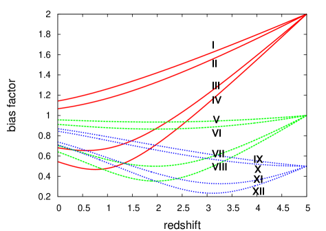
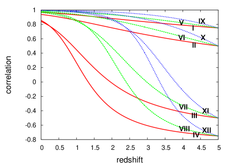
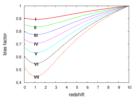
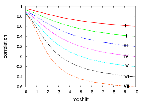
Figure 1: Evolution of the linear bias with no coupling between the galaxy species or to the dark matter present; the number of galaxies is hence conserved. One curve from the right and one curve from the left panel always belong together for one plotted model, twelve models are presented (roman numbers). The left panel shows the bias $b$ evolving for three quadruple of models from the initial values $b=2,1,0.5$ at redshift $z=5$ to $z=0$; the curves of each quadruple belong to initially (from upper to lower): $r=0.75,0.5,-0.5,-0.75$. In the right panel we depict the corresponding correlation parameter.

Figure 2: Evolution of the relative linear bias between two galaxy species , both starting off at $z=10$ with $b_{1}=b_{2}=4$. The correlation of one species to the dark matter is always $r_{1}=1$, whereas the second species has $r_{2}=0.6,0.4,0.2,0.0,-0.2,-0.4,-0.6$ for the curves in the left panel (upper to lower). The initial correlations between the galaxies where chosen to be $r_{12}=0.6,0.4,0.2,0.0,-0.2,-0.4,-0.6$. The left panel plots the evolution of $b_{12}$, the right panel $r_{12}$, same roman numbers correspond to one model. No coupling is present, hence the galaxy number is conserved.

2.5 Bias evolution without interaction

With no interaction present, $\Phi_{i}=0$, the model treats the same case as in the second section of TP98. Fig. 2 shows a diagram similar to the one in their paper: it can be seen that an initially biased galaxy distribution is more and more relaxing towards the dark matter distribution, asymptotically closing in to $r=1$ and $b=1$ (“debiasing”). That this is indeed a stationary state, i.e. $\frac{\partial b_{i}}{\partial t}=\frac{\partial r_{i}}{\partial t}=0$, can be seen from Eqs. (36) and (38) for which the only stationary solutions are $b_{i}=r_{i}=\pm 1$ (without interaction, hence $I^{1}_{i}=0$).

The second solution with $b_{i}=r_{i}=-1$ has to be excluded, because the bias factor is by definition always positive. The only possible way to be attracted by this stationary point is that we have $r_{i}=-1$ at all time. For all other values $r_{i}>-1$, the correlation parameter is an increasing function with time, inevitably approaching the other stationary solution. This peculiarity is therefore avoided if we exclude $r_{i}=-1$ as initial condition.

The bias between two galaxy populations also has a stationary solution at $b_{ij}=b_{i}/b_{j}=r_{ij}=1$. This follows from Eqs. (37) and (39) ($I^{2}_{i}=I^{3}_{ij}=0$). Fig. 2 shows as an illustration the evolution of the relative bias between two galaxy populations while they are getting debiased with respect to the dark matter.

3 Linear and quadratic interaction rates $\Phi_{i}$

Table 1: Three tables listing the contributions of the different couplings in Sect. 3 to the interaction terms $I^{0}_{i}$, $I^{2}_{i}$, $I^{3}_{ij}$ and the mean interaction rate $\big{\langle}\Phi_{i}\big{\rangle}$ sorted by the coupling constants; they are required by Eqs. (36) to (40). $A_{i}$ corresponds to a constant galaxy production/destruction, $B_{i}^{l}$ couples galaxy field $n_{l}$ to $n_{i}$ (linear), $C_{i}$ $n_{i}$ to the dark matter field $\rho_{\rm m}$ (linear), $D_{i}^{ls}$ couples $n_{l}$ and $n_{s}$ to $n_{i}$ (quadratic), $E_{i}$ couples $\rho_{\rm m}^{2}$ to $n_{i}$ (quadratic), and $F_{i}^{l}$ couples $n_{i}$ to $n_{l}$ and the dark matter field $\rho_{\rm m}$ (quadratic). The whole expression contributing is the product between the coupling constant, first column, and the expression in the second column or third column. Different contributions from different couplings are just added; we are using Einstein’s summation convention for the variables $l$ and $s$. Note that we have the special case $r_{ii}\equiv 1$ by definition of the correlation parameter. The bias parameters $\widehat{b_{i}r_{i}}$ and $\widehat{b_{j}b_{j}r_{ij}}$, and $\big{\langle}\delta_{\rm m}^{2}\big{\rangle}$ are explained in section 3. They are only needed for modelling the mean galaxy density in the presence of quadratic couplings.

term	$\bf I^{0}_{i}$	$\bf\big{\langle}\Phi_{i}\big{\rangle}$
$\bf A_{i}$	$0$	$1$
$\bf B_{i}^{l}$	$\frac{\bar{n}_{l}}{\bar{n}_{i}}r_{il}b_{l}$	$\bar{n}_{l}$
$\bf C_{i}$	$\frac{1}{\bar{n}_{i}}r_{i}$	$1$
$\bf D_{i}^{ls}$	$\frac{\bar{n}_{l}\bar{n}_{s}}{\bar{n}_{i}}r_{li}b_{l}+r_{si}b_{s}$	$\left(1+\widehat{b_{l}b_{s}r_{ls}}\big{\langle}\delta_{\rm m}^{2}\big{\rangle}\right)\bar{n}_{l}\bar{n}_{s}$
$\bf E_{i}$	$\frac{2}{\bar{{n}}_{i}}r_{i}$	$1+\big{\langle}\delta_{m}^{2}\big{\rangle}$
$\bf F_{i}^{l}$	$\frac{\bar{{n}}_{l}}{\bar{{n}}_{i}}\left(r_{i}+r_{li}b_{l}\right)$	$\left(1+\widehat{b_{l}r_{l}}\big{\langle}\delta_{\rm m}^{2}\big{\rangle}\right)\bar{n}_{l}$

term	$\bf I^{2}_{i}$
$\bf A_{i}$	0
$\bf B_{i}^{l}$	$\frac{\bar{{n}}_{l}}{\bar{{n}}_{i}}\frac{b_{l}}{b_{i}}\left(r_{l}-r_{i}r_{li}\right)$
$\bf C_{i}$	$\frac{1}{\bar{{n}}_{i}}\frac{1}{b_{i}}\left(1-r_{i}^{2}\right)$
$\bf D_{i}^{ls}$	$\frac{\bar{{n}}_{l}\bar{{n}}_{s}}{\bar{{n}}_{i}}\frac{1}{b_{i}}\left(\left[r_{l}-r_{li}r_{i}\right]b_{r}+\left[r_{s}-r_{si}r_{i}\right]b_{s}\right)$
$\bf E_{i}$	$\frac{2}{\bar{{n}}_{i}}\frac{1}{b_{i}}\left(1-r_{i}^{2}\right)$
$\bf F_{i}^{l}$	$\frac{\bar{{n}}_{l}}{\bar{{n}}_{i}}\frac{1}{b_{i}}\left(1-r_{i}+\left[r_{l}-r_{li}\right]b_{l}\right)$

term	$\bf I^{3}_{ij}$
$\bf A_{i}$	0
$\bf B_{i}^{l}$	$\frac{\bar{{n}}_{l}}{\bar{{n}}_{i}}\frac{b_{l}}{b_{i}}\left(r_{lj}-r_{li}r_{ij}\right)$
$\bf C_{i}$	$\frac{1}{\bar{{n}}_{i}}\frac{1}{b_{i}}\left(r_{j}-r_{i}r_{ij}\right)$
$\bf D_{i}^{ls}$	$\frac{\bar{{n}}_{l}\bar{{n}}_{s}}{\bar{{n}}_{i}}\frac{1}{b_{i}}\left(\left[r_{lj}-r_{ij}r_{li}\right]b_{l}+\left[r_{sj}-r_{ij}r_{si}\right]b_{s}\right)$
$\bf E_{i}$	$\frac{2}{\bar{{n}}_{i}}\frac{1}{b_{i}}\left(r_{j}-r_{i}r_{ij}\right)$
$\bf F_{i}^{l}$	$\frac{\bar{{n}}_{l}}{\bar{{n}}_{i}}\frac{1}{b_{i}}\left(\left[r_{lj}-r_{li}r_{ij}\right]b_{l}+r_{j}-r_{i}r_{ij}\right)$

To be specific about the interaction term, we make the following Ansatz for $\Phi_{i}$, namely a Taylor expansion in $n_{i}$ and $\rho_{\rm m}$ up to second order:

$$\Phi_{i}=A_{i}+B_{i}^{r}n_{r}+\hat{C}_{i}\rho_{\rm m}+D_{i}^{rs}n_{r}n_{s}+\hat{E}_{i}\rho_{\rm m}^{2}+\hat{F}_{i}^{r}\rho_{\rm m}n_{r}\;.$$ (42)

$A_{i}$, $B^{r}_{i}$, $\hat{C}_{i}$, $D^{rs}_{i}$, $\hat{E}_{i}$ and $\hat{F}_{i}^{r}$ are phenomenological coupling constants. Note that we are using the Einstein summing convention that abbreviates e.g. the expression $\sum_{rs}D^{rs}_{i}n_{r}n_{s}$ through $D^{rs}_{i}n_{r}n_{s}$. As before, we skip the position arguments of the density fields.

This particular $\Phi_{i}$ is motivated by the idea that locally the galaxy density may be changed - apart from converging or diverging bulk flows - by galaxy collisions or mergers with interaction rates proportional to the product of the density fields involved ($D_{i}^{rs}$, $\hat{E}_{i}$ and $\hat{F_{i}^{r}}$). In addition, we also include all lower order terms, like, for instance, a constant rate of galaxy production $A_{i}$ or a rate that is linear with some density field ($B_{i}^{r}$ and $\hat{C}_{i}$). As the non-linear, quadratic couplings linear couplings may also have a physical interpretation in this context: a galaxy of one population is with a constant probability - independent of its environment- transformed into a member of another population (passive evolution).

Actually needed inside Eqs. (36) to (40) are, however, not the $\Phi_{i}$ but the interaction terms in Eqs. (41). Those are mainly functions of the interaction correlators $\Big{\langle}\tilde{\Phi}_{i}\tilde{\delta}_{j}^{\ast}\Big{\rangle}^{\prime}$ and $\Big{\langle}\tilde{\Phi}_{i}\tilde{\delta}_{m}^{\ast}\Big{\rangle}^{\prime}$ whose evaluation can be found in Appendix C.

We have to evaluate the interaction rate per unit volume in Eq. (40), too:

$$\big{\langle}\Phi_{i}\big{\rangle} = A_{i}+C_{i}+E_{i}+\left(B_{i}^{r}+F_{i}^{r}\right)\bar{n}_{r}+D_{i}^{rs}\bar{n}_{r}\bar{n}_{s}$$

$$+ D_{i}^{rs}\bar{n}_{r}\bar{n}_{s}\big{\langle}\delta_{r}\delta_{s}\big{\rangle}+E_{i}\big{\langle}\delta_{\rm m}^{2}\big{\rangle}+F_{i}^{r}\bar{n}_{r}\big{\langle}\delta_{\rm m}\delta_{r}\big{\rangle}\;,$$

where the mean dark matter density $\bar{\rho}_{\rm m}$ has been absorbed inside the coupling constants (Appendix C). Note that the density contrasts here are in real space. For linear couplings only, the evolution of the mean volume density of galaxies is apparently independent from the way the galaxies are clustered, because then Eq. (40) only depends on $\bar{n}_{i}$. Quadratic couplings, however, introduce the terms like $\big{\langle}\delta_{i}\delta_{j}\big{\rangle}$, so that the mean density evolution gets linked to the correlations between $\delta_{i}$ and $\delta_{\rm m}$, and the fluctuations of these fields. The meaning of this is, that under quadratic couplings the mean density of highly clustered galaxies evolves in a different way than a completely homogeneous galaxy field.

To develop the last equation a bit further, we now would like to express the (real space) fluctuations/correlations $\big{\langle}\delta_{i}\delta_{j}\big{\rangle}$ and $\big{\langle}\delta_{\rm m}\delta_{j}\big{\rangle}$ in terms of linear bias parameters and the dark matter density fluctuations $\big{\langle}\delta_{\rm m}^{2}\big{\rangle}$ only. Expanding the correlator $\big{\langle}\delta_{i}\delta_{j}\big{\rangle}$ in Fourier space employing Eqs. (2) gives

$$\big{\langle}\delta_{i}\delta_{j}\big{\rangle} = \frac{1}{2\pi^{2}}\int dk\leavevmode\nobreak\ k^{2}\left|\tilde{W}\left(k\right)\right|^{2}b_{i}\left(k\right)b_{j}\left(k\right)r_{ij}\left(k\right)P_{\rm m}\left(k\right)$$ (44)

$$= \widehat{b_{i}b_{j}r_{ij}}\;\big{\langle}\delta_{\rm m}^{2}\big{\rangle}$$

$$\big{\langle}\delta_{\rm m}^{2}\big{\rangle} = \frac{1}{2\pi^{2}}\int dk\leavevmode\nobreak\ w\left(k\right)\;,$$ (45)

using the definitions

$$\widehat{b_{i}b_{j}r_{ij}} \equiv \frac{\int dk\leavevmode\nobreak\ w\left(k\right)b_{i}\left(k\right)b_{j}\left(k\right)r_{ij}\left(k\right)}{\int dk\leavevmode\nobreak\ w\left(k\right)}$$ (46)

$$w\left(k\right) \equiv k^{2}\left|\tilde{W}\left(k\right)\right|^{2}P_{\rm m}\left(k\right)\;.$$ (47)

We have introduced a window function $\tilde{W}\left(k\right)$ to account for the fact that the density fields $\delta_{i}$ and $\delta_{\rm m}$ entering the interaction rate $\Phi_{i}$ as quadratic coupling terms in general may be smoothed with some kernel $W\left(r\right)$. It is, for instance, plausible that fluctuations of the fields much smaller than the typical size of a galaxy are not relevant for galaxy interactions, although mathematically the density fields may have an infinite resolution. In that particular case, $W\left(r\right)$ could be modelled as a top hat of some typical width $R_{\rm int}$ with the following $\tilde{W}\left(k\right)$

$$\tilde{W}\left(y\right)=\frac{3}{y^{3}}\left(\sin{y}-y\cos{y}\right)\;,$$ (48)

with $y\equiv kR_{\rm int}$ (e.g. Peacock 2001, page 500).

The expression $\widehat{b_{i}b_{j}r_{ij}}$ is the weighted mean of $b_{i}\left(k\right)b_{j}\left(k\right)r_{ij}\left(k\right)$ over all scales. Fig. (4) shows the weights $w\left(k\right)$ for some redshifts and one particular cosmological model. In the plotted redshift range, the weight peaks at about $1$ Mpc $h^{-1}$, but has a considerable width though; that is assuming that $R_{\rm int}\ll 1$ Mpc $h^{-1}$. In an analogue manner, we obtain

$$\big{\langle}\delta_{i}\delta_{\rm m}\big{\rangle}=\widehat{b_{i}r_{i}}\;\big{\langle}\delta_{\rm m}^{2}\big{\rangle};\;\;\widehat{b_{i}r_{i}}\equiv\frac{\int dk\leavevmode\nobreak\ w\left(k\right)b_{i}\left(k\right)r_{i}\left(k\right)}{\int dk\leavevmode\nobreak\ w\left(k\right)}\;.$$ (49)

Eq. (3) hence can be written as

$$\big{\langle}\Phi_{i}\big{\rangle} = A_{i}+C_{i}+E_{i}+B_{i}^{r}\bar{n}_{r}$$

$$+ D_{i}^{rs}\left[1+\widehat{b_{r}b_{s}r_{rs}}\big{\langle}\delta_{\rm m}^{2}\big{\rangle}\right]\bar{n}_{r}\bar{n}_{s}$$

$$+ F_{i}^{s}\left[1+\widehat{b_{s}r_{s}}\big{\langle}\delta_{\rm m}^{2}\big{\rangle}\right]\bar{n}_{s}+E_{i}\big{\langle}\delta_{\rm m}^{2}\big{\rangle}\;.$$

Table 1 summarises the final result for $I^{0}_{i}$, $I^{2}_{i}$, $I^{3}_{ij}$ and $\big{\langle}\Phi_{i}\big{\rangle}$ as list of contributions stemming from the various linear and quadratic interaction terms in (42). As both the interaction terms and the mean galaxy interaction rate are linear in $\Phi_{i}$, all different coupling contributions are simply added in order to obtain the final terms.

To give an example, assume we would like to couple linearly a galaxy population $n_{1}$ to the galaxy population $n_{2}$; this is an interaction of the $B_{i}^{j}$ type. In our notation, $\left(b_{1}\leavevmode\nobreak\ r_{1}\right)$, $\left(b_{2}\leavevmode\nobreak\ r_{2}\right)$ and $\left(b_{12}\leavevmode\nobreak\ r_{12}\right)$ are the linear bias parameters of population $n_{1}$ with respect to the dark matter, of population $n_{2}$ with respect to the dark matter and of population $n_{1}$ with respect to population $n_{2}$ respectively. According to table 1, the interaction terms are explicitly (after some algebra using $r_{11}=r_{22}=1$ and $r_{12}=r_{21}$):

$$I^{0}_{1}=B_{1}^{1}\leavevmode\nobreak\ b_{1}+\frac{\bar{n}_{2}}{\bar{n}_{1}}B_{1}^{2}\leavevmode\nobreak\ r_{12}b_{2}; I^{0}_{2}=B_{2}^{2}\leavevmode\nobreak\ b_{2}+\frac{\bar{n}_{1}}{\bar{n}_{2}}B_{2}^{1}\leavevmode\nobreak\ r_{12}b_{1}$$

$$I_{1}^{2}=B_{1}^{2}\leavevmode\nobreak\ \frac{\bar{n}_{2}b_{2}}{\bar{n}_{1}b_{1}}\left(r_{2}-r_{1}r_{12}\right); I_{2}^{2}=B_{2}^{1}\leavevmode\nobreak\ \frac{\bar{n}_{1}b_{1}}{\bar{n}_{2}b_{2}}\left(r_{1}-r_{2}r_{12}\right)$$

$$I^{3}_{12}=B_{1}^{2}\leavevmode\nobreak\ \frac{\bar{n}_{2}b_{2}}{\bar{n}_{1}b_{1}}\left(1-r_{12}^{2}\right); I^{3}_{21}=B_{2}^{1}\leavevmode\nobreak\ \frac{\bar{n}_{1}b_{1}}{\bar{n}_{2}b_{2}}\left(1-r_{12}^{2}\right)$$

$$I^{3}_{11}=0; I^{3}_{22}=0$$

$$\big{\langle}\Phi_{1}\big{\rangle}=B_{1}^{1}\bar{n}_{1}+B_{1}^{2}\bar{n}_{2}; \big{\langle}\Phi_{2}\big{\rangle}=B_{2}^{1}\bar{n}_{1}+B_{2}^{2}\bar{n}_{2}$$

$B_{1}^{1}$ and $B_{2}^{2}$ couple the galaxy population to themselves and are therefore zero if solely couplings between $n_{1}$ and $n_{2}$ are allowed. If the number of galaxies $\bar{n}_{1}+\bar{n}_{2}$ is conserved by this kind of interaction, thus $\frac{\partial\bar{n}_{1}}{\partial t}=\frac{\partial\bar{n}_{2}}{\partial t}=0$, then we have the further constraint $B_{1}^{2}=-B_{2}^{1}$ as can be seen from Eq. (40). In case that two galaxies of $i=1$ “merge” to produce one $i=2$ galaxy, we have the constraint $B_{1}^{2}=-\frac{1}{2}B_{2}^{1}$.

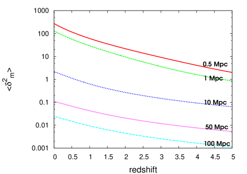
Figure 3: Estimated fluctuations $\big{\langle}\delta_{m}^{2}\big{\rangle}$, Eq. (45), of the dark matter density field for different cutoffs $R_{\rm int}$ using the PD96 prescription for the non-linear clustering regime; see Sect. 4 for cosmological parameters.

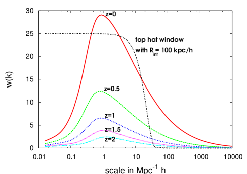
Figure 4: Weighting factors $w\left(k\right)$ (in arbitrary units, see Eq. 47) for different redshifts, the window $\tilde{W}\left(k\right)$ was set to one. The weight maximum stays roughly at the same scale in the plotted redshift interval; the peak is quite broad however. Also plotted here is the window function $\left|\tilde{W}\left(k\right)\right|^{2}$ (not normalised) of a top hat $W\left(r\right)$ with $R_{\rm int}=100\leavevmode\nobreak\ \rm kpc/h$ which would cut-off the weights beyond $k_{\rm int}/2\pi=10\leavevmode\nobreak\ \rm Mpc^{-1}h$. See Sect. 4 for cosmological parameters; the PD96 prescription was used for non-linear regime.

4 Toy models

In this section, we present a few examples to illustrate the impact of interactions on the evolution of the linear bias parameters. These include the bias of each galaxy population with respect to both the dark matter and all other populations. For predicting the bias evolution on large scales, we incorporate the model Eqs. (36) to (40).

Owing to the large number of free parameters and ways to combine them, there are many models to look at. To explore some of them, we focus on two galaxy populations and “switch on” only one parameter out of $A_{i}-F_{i}^{j}$ in Eq. (42) while setting the others to zero. This allows us to look at the effect of the coupling parameters separately.

The evolution is plotted in redshift. Therefore, we have to transform the derivatives with respect to cosmic time $t$

$$\frac{\partial}{\partial t}=\frac{\partial a}{\partial t}\frac{\partial z}{\partial a}\frac{\partial}{\partial z}=-\left.\frac{H\left(a\right)}{a}\right|_{a=\left(1+z\right)^{-1}}\frac{\partial}{\partial z}\;.$$ (51)

The dark matter growth rate defined in Eq. (32) is accordingly as function of redshift

$$R\left(z\right)=R\left(t\right)|_{t=t\left(z\right)}=\left.2\left[aH\left(a\right)\frac{\partial\ln{D_{+}}}{\partial a}\right]\right|_{a=\left(1+z\right)^{-1}}$$ (52)

which then may be evaluated using Eq. (30) ($H\left(a\right)$ is defined in Eq. 6).

It may be useful to have these expressions for a simple cosmology, like for the Einstein-de Sitter Universe with $D_{+}=a$ and $H\left(a\right)=H_{0}a^{-3/2}$ ($a\equiv 1$ at $z=0$)

$$\left.\begin{array}[]{lll}R\left(z\right)&=&+2H_{0}\left(1+z\right)^{3/2}\\ \ \frac{\partial}{\partial t}&=&-H_{0}\left(1+z\right)^{5/2}\frac{\partial}{\partial z}\end{array}\right\}{\rm Einstein-de\leavevmode\nobreak\ Sitter}\;.$$ (53)

Our cosmology in the examples stated here is a $\Lambda$CDM model with $\Omega_{\rm m}=0.3$, $\Omega_{\Lambda}=0.7$, $\rm H_{0}=70\leavevmode\nobreak\ \rm kms^{-1}Mpc^{-1}$. Furthermore, a scale-invariant $n=1$ Harrison Zel’dovich spectrum for the primordial fluctuations is assumed. For the 3-D power spectrum of the matter fluctuations we use the fitting formula of Bardeen et al. (1986) for the transfer function, and the Peacock & Dodds (1996), hereafter PD96, description for the evolution in the non-linear regime. The power spectrum normalisation is parameterised with $\sigma_{8}=0.9$ and the shape parameter assumed to be $\Gamma=0.21$ (the 3-D matter fluctuations spectrum is needed for the quadratic coupling models only).

For the discussion of the toy models see section 5.

4.1 Constraints on the correlation parameter

As initial condition, one can set the bias parameter $b_{i}$ freely. The relative bias $b_{ij}$ between the different galaxy populations is thereby also fixed, namely $b_{ij}=b_{i}/b_{j}$.

The choice of the initial conditions of the correlation coefficients $\left(r_{i}\leavevmode\nobreak\ r_{ij}\right)$ is not free, however. For example, we cannot demand population A to be 100 percent correlated to both population B and population C, but, at the same time, population B to be not correlated to C. To be more general, we arrange the density contrasts of the dark matter and $N$ galaxy fields in terms of one single vector

$${\bf x}\left({\bf k}\right)=\left(\tilde{\delta}_{\rm m}\left({\bf k}\right)\leavevmode\nobreak\ \leavevmode\nobreak\ \tilde{\delta}_{1}\left({\bf k}\right)\leavevmode\nobreak\ \leavevmode\nobreak\ ...\leavevmode\nobreak\ \leavevmode\nobreak\ \tilde{\delta}_{\rm N}\left({\bf k}\right)\right)^{\rm t}\;,$$ (54)

with ${\bf x}^{\rm t}$ being the transpose of ${\bf x}$. Concerning the bias parameter, we are restricted by the fact that the covariance matrix ${\bf C}\left({\bf k}\right)=\Big{\langle}{\bf x}\left({\bf k}\right){\bf x}^{\rm t}\left({\bf k}^{\prime}\right)\Big{\rangle}^{\prime}$ has to be positive semidefinite, thus the determinant of

$${\bf C}\left({\bf k}\right)=$$

$$P_{\rm m}\left({\bf k}\right)\left(\begin{array}[]{lllll}1&r_{1}b_{1}&r_{2}b_{2}&...&r_{N}b_{N}\\ r_{1}b_{1}&b_{1}^{2}&b_{1}b_{2}r_{12}&...&b_{1}b_{N}r_{1N}\\ ...&...&...&...&...\\ r_{N}b_{N}&b_{1}b_{N}r_{1N}&...&...&b_{N}^{2}\end{array}\right)$$ (59)

has to be greater than or equal to zero (as before, we have left out the ${\bf k}$-dependence of the bias parameter in the notation).

For three random fields (or two galaxy populations plus the dark matter field), this statement is equivalent to

$$2r_{1}r_{2}r_{12}\geq r_{1}^{2}+r_{2}^{2}+r_{12}^{2}-1\;,$$ (60)

if the definitions of ${\bf C}$, $r_{1}$, $r_{2}$, $r_{12}$ are used (calculation not shown here). It holds for all scales and the large-scale parameter considered in particular. Going back to the example above, it follows immediately from this equation that if we fix two of the three correlation coefficients with one, say $r_{1}=r_{2}=1$, the third automatically is also forced to be one. Even more general, if only one of the correlations is set to one, say $r_{1}$, then the other two have to be equal, since we are told by the above constraint that

$$\left(r_{2}-r_{12}\right)^{2}\leq 0\;.$$ (61)

Already for four random fields (or three galaxy populations plus the dark matter field) this condition of positive semi-definiteness becomes rather lengthy:

$$r_{1}^{2}r_{23}^{2}+r_{2}^{2}r_{13}^{2}+r_{3}^{2}r_{12}^{2}+$$ (62)

$$2\big{[}r_{1}r_{2}r_{12}+r_{1}r_{3}r_{13}+r_{2}r_{3}r_{23}+r_{12}r_{13}r_{23}-$$

$$r_{1}r_{2}r_{13}r_{23}-r_{1}r_{3}r_{12}r_{23}-r_{2}r_{3}r_{12}r_{13}\big{]}$$

$$\geq r_{1}^{2}+r_{2}^{2}+r_{3}^{2}+r_{12}^{2}+r_{13}^{2}+r_{23}^{2}-1\;.$$

By setting all correlations with the third population to zero ($r_{3}=r_{13}=r_{23}=0$), one can see that this reduces to the forgoing inequality (60). Thus, the constraint for three galaxy populations is a more general expression that simplifies to the condition for two populations if one of the three galaxy populations is not all correlated to the two others and the dark matter; it is in a statistical sense disconnected from the others.

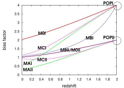
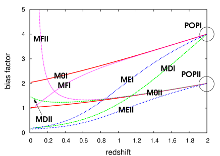
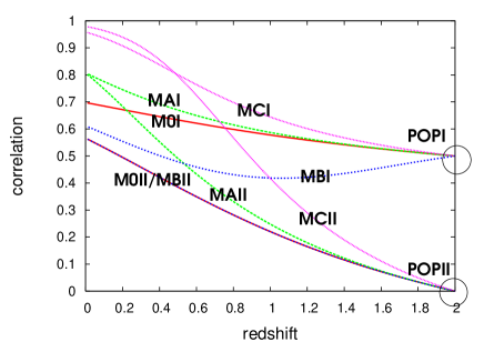
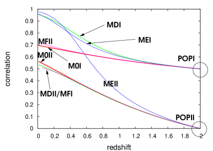
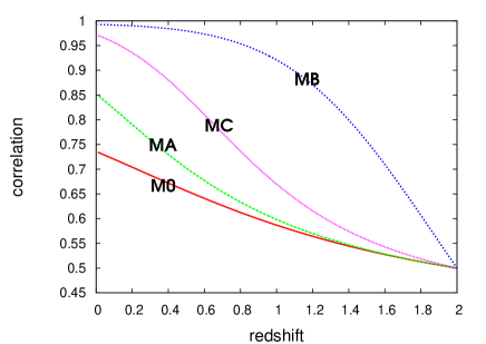
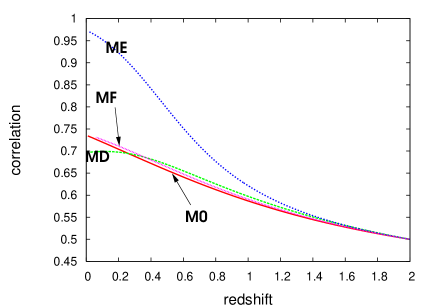
Figure 5: Example evolutionary tracks of two galaxy populations POPI and POPII subject to different “interactions”. All scenarios share same initial conditions at $z=2$ (POPI: $b_{I}=4$,$r_{I}=0.5$; POPII: $b_{II}=2$, $r_{II}=0$; $r_{I/II}=0.5$). Depicted are as a function of redshift (upper to lower row): bias factors $b_{I}$ and $b_{II}$ with respect to dark matter, correlations $r_{I}$ and $r_{II}$ to the dark matter field, and correlation $r_{I/II}$ between the two galaxy fields (Sects. 4.2 and 4.3 for details)
left column (linear couplings): (arbitrary units) M0: interaction free case; MA: constant creation of galaxies with $A_{I}=A_{II}=10$; MB: POPII galaxies being transformed to POPI galaxies with $B_{I}^{II}=-B_{II}^{II}=10$; MC: linear coupling of both POPI and POPII to dark matter field with $C_{I}=C_{II}=10$
right column (quadratic couplings): (arbitrary units) M0: interaction free evolution; MD: “colliding” POPII galaxies are transfered to POPI with $D_{I}^{II\leavevmode\nobreak\ II}=-D_{II}^{II\leavevmode\nobreak\ II}=10^{-4}$; ME: both populations are coupled to $\rho_{m}^{2}$ with $E_{I}=E_{II}=1$; MF: POPI galaxies are produced by $\Phi_{I}\propto{\rm n}_{II}\rho_{m}$ as much as POPII galaxies are destroyed, $F_{I}^{II}=-F_{II}^{II}=0.1$.

4.2 Linear couplings

We first focus on the linear couplings by the $A_{i}$, $B_{i}^{j}$ and $C_{i}$ interaction terms. For these three scenarios (MA, MB and MC respectively), we plot in Fig. 5 the evolutionary tracks of the linear bias of two different galaxy populations.

The first population, hereafter POPI, has initially at redshift $z=2$ a bias factor $b_{I}=4$ and correlation $r_{I}=0.5$ with respect to the dark matter. The second population, hereafter POPII, has $b_{II}=2$ and $r_{II}=0$ at $z=2$; it is thus initially not correlated to the dark matter. The relative correlation between POPI and POPII we set to $r_{I/II}=0.5$, well below maximum possible value of $r_{I/II}=0.87$ (according to Eq. 60). The number density of galaxies is not constant due to the interaction (not plotted).

For the scenario MB, we assume that POPI is coupled to POPII such that galaxies are transfered from POPII to POPI keeping the overall galaxy number unchanged, thus $B_{I}^{II}=-B_{II}^{II}$. Moreover, for that particular scenario we increase the initial number of POPII galaxies so that $\bar{n}_{II}=10\bar{n}_{I}$. In all other scenarios we used $\bar{n}_{I}=\bar{n}_{II}$. Everywhere we use $\bar{\rm n}_{I}=1$ in arbitrary units.

4.3 Quadratic couplings

For the toy models in this section, we assume that the bias parameters are scale-independent, so that $\widehat{b_{i}b_{j}r_{ij}}=b_{i}b_{j}r_{ij}$ and $\widehat{b_{j}r_{ij}}=b_{j}r_{ij}$, where $\left(b_{i}\leavevmode\nobreak\ b_{ij}\leavevmode\nobreak\ r_{i}\leavevmode\nobreak\ r_{ij}\right)$ are the large-scale bias parameter as described in Sect. 2.4. Furthermore, we model the window $\tilde{W}\left(k\right)$ (see Sect. 3) as a constant function with a cutoff beyond a typical interaction scale $k_{\rm int}=2\pi/R_{\rm int}$, here chosen to be $R_{\rm int}=1\leavevmode\nobreak\ \rm Mpc$. We use the PD96 approximation for the non-linear evolution of the dark matter power spectrum to estimate

$$\big{\langle}\delta_{m}^{2}\big{\rangle}=\frac{1}{2\pi^{2}}\int_{0}^{k_{\rm int}}dk\leavevmode\nobreak\ k^{2}\leavevmode\nobreak\ P_{\rm m}\left(k\right)\;.$$ (63)

Fig. 3 shows the estimates for different scales.

Fig. 5 shows examples of non-linear (quadratic) couplings as conveyed by the interaction terms $D_{i}^{rs}$, $E_{i}$ and $F_{i}^{r}$. These interactions lead to the scenarios MD, ME and MF respectively. Again, as in the foregoing section, we have two galaxy populations POPI and POPII with the aforementioned initial conditions. For the mean galaxy density we set $\bar{n}_{II}=100\bar{\rm n}_{I}$, except for ME where we assumed the same initial density for both populations.

As before, we do not plot the evolution of the number densities. MD couples POPI to POPII such that galaxies are added to POPI by “collisions” of POPII galaxies, while the same amount of galaxies is taken from POPII ($D_{I}^{II\leavevmode\nobreak\ II}=-D_{II}^{II\leavevmode\nobreak\ II}$, all others are zero). MF transfers galaxies from POPII to POPI by a quadratic coupling of the dark matter and POPII density field, hence creating new POPI galaxies everywhere where the density of both the dark matter and POPII galaxies is high. Here, we also adjust the coupling constants $F_{i}^{j}$ such that the overall galaxy density remains constant ($F_{I}^{II}=-F_{II}^{II}$).

5 Discussion and conclusions

Taking the hypothesis for granted that the bulk flow of galaxies is identical to the bulk flow of the dark matter field, we derive a set of differential equations that describe the evolution of the two-point correlations between different galaxy populations and the dark matter density field in terms of correlation power spectra (Eqs. 33, 2.3 and 12). Incorporated into this model is an “interaction” $\Phi_{i}$ that allows for the destruction or creation of galaxies; in this paper, the term interaction is used equivalently to a local change of the galaxy number density. It may have explicit time dependence.

The model is valid only on scales where three point correlations of all cosmological fields (density and velocity fields) are negligible. This is fulfilled on large scales where the fields are Gaussian due to the initial conditions of structure formation at high redshifts (as seen in the CMB) and due to the fact that the field evolution is essentially linear on large scales. On small scales, this assumption is definitely wrong, because gravitational instability has been destroying Gaussianity proceeding gradually from smallest to larger scales. The present stage of structure formation in the local Universe is such that this transition form linear to non-linear scales occurs at about $10$ Mpc $h^{-1}$; at earlier times, this scale was smaller.

We closely study an interaction rate $\Phi_{i}$ that is a local function of the (smoothed) dark matter density field and the galaxy number density fields up to second order; within the model, the choice of the interaction is completely free though. With this interaction, we introduce the coupling constants $A_{i}$, $B_{i}^{r}$, $C_{i}$, $D_{i}^{rs}$, $E_{i}$ and $F_{i}^{r}$ (see Eq. 42). Generally, this interaction term may be pictured as the Taylor expansion of some complicated interaction $\Phi_{i}\left({\rm n}_{j},\rho_{\rm m}\right)$ up to second order. Nevertheless, some of the terms associated with the coupling constants taken alone bear a simple interpretation. $D_{i}^{rs}$ may be used to describe interaction rates of galaxy-galaxy collisions or mergers. Merging is an important process in the currently favoured $\Lambda$CDM Universe (e.g. Lacey & Cole 1993). Linear couplings between the galaxy fields, $B_{i}^{r}$, have a physical analogue as well: they describe processes that transfer a certain fraction of one galaxy population to another population per volume and time, making the local creation/destruction rate of galaxies proportional to the local density of the other population (passive evolution). A constant production/destruction rate of galaxies, $A_{i}$, is just a special case as it acts like a linear coupling to a completely homogeneous field of galaxies.
The 2nd order couplings between dark matter and galaxy fields, $E_{i}$ and $F_{i}^{r}$, and the linear coupling between dark matter and galaxies, $C_{i}$, may be used, for instance, to describe formation processes that directly require the presence of dark matter overdensities, albeit the interpretation of these terms alone is less clear. At least, one can say that linear couplings to the dark matter field produce galaxies that are not biased with respect to the dark matter, while a quadratic coupling makes relatively more galaxies in overdensity regions.

General descriptions of a local stochastic bias like the one from Dekel & Lahav (1999) are based on the joint pdf of the (smoothed) density contrasts of the considered fields. Therefore - however the defined bias parameters may look like - they have to be function of the cumulants $\big{\langle}\delta_{i_{1}}^{n_{1}}...\delta_{i_{N}}^{n_{N}}\big{\rangle}_{c}$ of this pdf, so that these are the basic quantities that should be examined. Due to the Gaussianity of the fields on linear scales only the second order cumulants are non-vanishing and hence only the stochastic linear bias parameters in (2) are relevant; the first order cumulants vanish according to the definition of the density contrasts. Their evolution is described by means of Eqs. (36) to (40); Table 1 lists the interaction terms based on the interaction correlators for the 2nd order Taylor expansion of $\Phi_{i}$. Our model distinguishes between the linear bias $\left(b_{i}\leavevmode\nobreak\ r_{i}\right)$ of a galaxy population with respect to the dark matter field and the linear bias $\left(b_{ij}\leavevmode\nobreak\ r_{ij}\right)$ between two galaxy populations. The bias factor “$b$” can be pictured as the ratio of the clustering strengths of the two fields, whereas the correlation parameter “$r$” measures how strongly the peaks and valleys of the density fields coincide. Note, however, that also a possible non-linearity in the relation between $\delta_{i}$ and $\delta_{j}$ affects the correlation parameter (Dekel & Lahav 1999). On the large smoothing scales considered by this paper this is neglectable though.

For all fields perfectly correlated to the dark matter field, thus $r_{i}=r_{ij}=1$, the interaction terms $I^{2}_{i}$ and $I^{3}_{ij}$ always vanish and therefore all correlations $\left(r_{i}\leavevmode\nobreak\ r_{ij}\right)$ are “frozen in” according to Eqs. (38) and (39). In that case, the model reduces basically to Eq. (36) and (40) with all correlations set to one ($b_{ij}=b_{i}/b_{j}$):

$$\frac{\partial b_{i}}{\partial t}=R\left(t\right)\frac{1-b_{i}}{2}+\left.I^{1}_{i}\right|_{r_{i}=r_{ij}=1}\;.$$ (64)

The bias $b_{i}$ is then called deterministic, since there is no randomness in the relationship of the local density contrasts. For highly correlated fields, this can be a good approximation.

With no interaction present (Sect. 2.5), we obtain as TP98 and others a debiasing of an initially biased galaxy field; this makes the galaxy distribution looking more and more like the distribution of the underlying dark matter distribution (Figs. 2). The bias factor $b_{i}>1$ of a galaxy population that is less correlated to the dark matter field declines faster than a more correlated population (Fig. 2). The figure also demonstrates that differently correlated galaxy populations can temporarily evolve a relative bias factor $b_{ij}\neq 1$ with respect to each other even though they may have had $b_{ij}=1$ at some time and they are not interacting with each other. Moreover, characteristic for an only slightly correlated population, $r_{i}<1$, is an “overshoot” that makes the population antibiased, i.e. $b_{i}<1$, after some time. Later on, the bias factor increases again thereby producing a relative minimum in $b_{i}$. This minimum is clearly seen in Fig. 2; according to Eq. (36) it has to occur at the time where $r_{i}=b_{i}$, because $\frac{\partial b_{i}}{\partial t}$ vanishes there. On the other hand, this means that a possible local minimum of $b_{i}$ always has to be smaller than one since $r_{i}\leq 1$. In the absence of any interaction, the relative correlation is a monotonic, always increasing function; this is due to the rhs of Eq. (38) which always has a positive sign as long as $R\left(t\right)>0$.

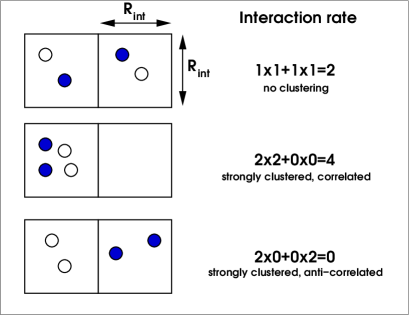
Figure 6: Sketch illustrating the effect of clustering and correlation on the mean interaction rate $\big{\langle}\Phi\big{\rangle}$, thus mean density evolution for quadratic couplings (“collisions”) $\Phi_{12}\propto n_{1}n_{2}$ between bright and dark particles. The space is divided into two cells only whose size corresponds to some typical interaction distance $R_{\rm int}$; interactions take place between particles within the same cell. From top to bottom: homogeneous distribution, strong clustering and high correlation between particles, strong clustering and high anti-correlation between particles. Strong clustering and high correlation obviously results in the highest interaction rate and hence influences the mean density evolution the most.

A few examples of linear couplings are plotted in Fig. 5. A linear coupling of a field “II” to a field “I” via $\Phi_{I}\propto n_{II}$ has the effect that the field of newly formed or recently destroyed galaxies type “I”, ${\rm d}n_{I}=\Phi_{I}{\rm d}t$, has the same bias than the field of the galaxies “II”. In case of the formation of galaxies “I” (positive sign in $\Phi_{I}$), this enriches the population “I” with new galaxies having the same correlations as the galaxies in field “II”. Therefore, the bias factor between “I” and “II” is being reduced while their correlation is being increased. A positive linear coupling to the dark matter field hence debiases a galaxy field quicker than without interaction (like the populations POPI and POPII in scenario MC). The linear coupling of POPII to POPI literally “drags” the population POPI towards POPII as can be seen in MBI, while POPII (MBII), even though loosing galaxies, shows the same behaviour as without interaction in M0II; this is because it is linearly coupled to itself. The interaction $A_{i}$ creates or destroys galaxies (depending on the sign) with the same rate everywhere; this can be pictured as a linear coupling to an absolutely homogeneous, fluctuation free field, having $b=0$ with respect to any other field. $I^{0}_{i}$ for $B_{i}^{j}$ in table 1 indeed reduces up to a constant to the $I^{0}_{i}$ for $A_{i}$, if we set $b_{j}=0$. It is therefore not surprising that a constant production of galaxies pulls the bias towards zero (see MAI and MAII), more and more suppressing the density fluctuations.

In conclusion, a linear coupling of a field “II” to field “I” only influences the bias evolution of “I” if “II” is biased with regard to “I”. In particular, a new population “I” being created solely from a linear coupling to some other population “II” can never become biased with respect to “II”. Early type galaxies that may be formed from spiral galaxies can therefore not be produced by a linear coupling to the spiral galaxy field if they are biased with respect to spirals as observations imply (Norberg et al. 2002). The fact that values for $\beta=\Omega_{\rm m}^{0.6}/b$ derived from the IRAS (preferentially spiral galaxies) and the ORS (optically selected galaxies) are consistent if a relative bias of $b_{\rm ORS}/b_{\rm IRAS}=1.4$ is assumed (Baker et al. 1998), also implies a bias between spirals and ellipticals on large scales. If this is the case then following the above arguments, ellipticals cannot simply be passively evolved spirals.

Quadratic interactions, physically interpreted as collisions or mergers, could do the job however. The reason is that the field of newly formed or recently destroyed galaxies of type “I”, coupled quadratically to “II” is proportional to $n_{II}^{2}$. These galaxies have therefore the bias factor of $n_{II}^{2}$, which in general is different from the bias factor of “II”; in fact, the density contrast $\delta_{\rm new}$ of the newly formed galaxies type “I” is then

$$\delta_{\rm new}=\frac{n_{II}^{2}}{\big{\langle}n_{II}^{2}\big{\rangle}}-1=\frac{2\delta_{II}+\delta_{II}^{2}-\big{\langle}\delta_{II}^{2}\big{\rangle}}{1+\big{\langle}\delta_{II}^{2}\big{\rangle}}\;.$$ (65)

Smoothing $\delta_{\rm new}$ out to sufficiently large scales gives

$$\delta_{\rm new}\approx\frac{2\delta_{II}}{1+\big{\langle}\delta_{II}^{2}\big{\rangle}}\;,$$ (66)

because $\delta_{II}^{2}$ smoothed on large scales is approximately $\big{\langle}\delta_{II}^{2}\big{\rangle}$ due to the ergodicity of the random field. Small fluctuations $\big{\langle}\delta_{II}^{2}\big{\rangle}\ll 1$ make the newly formed galaxies biased with a bias factor of about $b_{\rm new}\approx 2$ since $1+\big{\langle}\delta_{\rm II}^{2}\big{\rangle}\approx 1$ and $\delta_{\rm new}\approx 2\delta_{\rm II}$. For non-negligible fluctuations, on the other hand, this bias is roughly $b_{\rm new}=2/\left(1+\big{\langle}\delta_{\rm II}^{2}\big{\rangle}\right)$, thus taking a value between $0$ and $2$. This particular example, as a side remark, demonstrates nicely that interactions on very small scales can have an impact on the large-scale bias. As an example, see Fig. 7. Here we have a hypothetical population of galaxies (POPI) unbiased with respect to another population (POPII). Collisions of POPII galaxies add galaxies to POPI which then become biased or antibiased depending on whether $\big{\langle}\delta_{\rm II}^{2}\big{\rangle}\ll 1$ (scenario MX) or $\big{\langle}\delta_{\rm II}^{2}\big{\rangle}\gg 1$ (scenario MY).

Quadratic interactions, Eq. $(\ref{lindensity})$, present a challenging problem since one has to know the fluctuations of the density fields on small scales, or equivalently (see Eq. 44) the dispersion of the dark matter $\big{\langle}\delta_{\rm m}^{2}\big{\rangle}$, the linear bias parameters

$$\hat{{\bf b}}\equiv\left(\widehat{b_{i}b_{j}r_{ij}}\leavevmode\nobreak\ \widehat{b_{i}r_{j}}\right)$$ (67)

and a window function $W\left(r\right)$; the linear bias parameters $\hat{{\bf b}}$ are the weighted means of the $k$-space bias parameters over all scales $k$, or the (real space) bias parameter on a scale defined by $W\left(r\right)$ (like in Eq. 1). The window function actually defines what is meant by fluctuations on small scales by introducing a smoothing scale $R_{\rm int}$ of the (real space) fields entering $\Phi_{i}$, like for instance $n_{i}$ and $n_{j}$ in $\Phi_{i}\propto n_{i}n_{j}$. This scale is determined by the physical process underlying the interaction and therefore lies presumably deep in the non-linear regime. Why are these additional parameters needed for quadratic couplings? This can be seen by the following argument. One could think of the whole model volume being subdivided into small cubic cells with side length $R_{\rm int}$; a cell contains $N_{i}=n_{i}R_{\rm int}^{3}$ “particles” $n_{i}$. Roughly speaking, the model predicts the evolution of the correlations between the particle numbers $N_{i}$ of cells which are far apart (large scale) and the mean number of particles $\big{\langle}N_{i}\big{\rangle}$ inside the cells taking into account the gravitational field of the dark matter, its increasing clustering and the background cosmology. The interaction term $\Phi_{i}$ changes the number of galaxies $N_{i}$ inside a particular cell depending on the number of galaxies and/or dark matter mass present in the same cell by ${\rm d}N_{i}=R_{\rm int}^{3}\Phi_{i}{\rm d}t$. For linear couplings $\Phi_{i}\propto n_{j}$, the size of these cells does not have an impact on $\big{\langle}\dot{N}_{i}\big{\rangle}$ and thus $\big{\langle}\dot{n}_{i}\big{\rangle}$ since $\big{\langle}\Phi_{i}\big{\rangle}$ depends only on the total number of particles of all cells; hence $R_{\rm int}$ does not turn up in the model Eq. (40). For non-linear couplings, however, the mean interaction rate indeed depends on how the particles are distributed among the cells which is expressed by $\hat{{\bf b}}$.

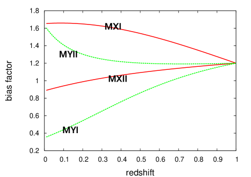
Figure 7: Evolutionary tracks of the bias factor with respect to the dark matter of two galaxy populations POPI and POPII for two scenarios MX and MY (initially at $z=1$: deterministic bias $b_{I}=b_{II}=1.2$, $\bar{n}_{I}=1$ and $\bar{n}_{II}=10^{-1}$). Both scenarios assume that collisions of POPII galaxies create POPI with $D_{I}^{II\leavevmode\nobreak\ II}=-D_{II}^{II\leavevmode\nobreak\ II}\equiv D$; colliding galaxies are removed. MX: sets $\big{\langle}\delta_{\rm m}^{2}\big{\rangle}=0$ or equivalently $\widehat{b_{I}b_{II}r_{I/II}}=0$ and $D=0.1$; MY: sets $\big{\langle}\delta_{\rm m}^{2}\big{\rangle}$ according to Fig. 3 with $\rm R_{\rm int}=1$Mpc and $D=0.01$ in order to have roughly the same evolution of $\bar{n}_{I}$ and $\bar{n}_{II}$ as MX.

To be able to explore a toy model including quadratic couplings, we made the assumption that the small-scale bias parameters are identical to the bias parameters on large scales; we hence assumed no scale-dependence for the linear bias. In fact, this is not what is expected for some galaxy populations: on large scales early and late type galaxies share approximately the same distribution (more galaxies inside super-clusters, less in the voids outside), while on smaller, cluster-scales early and late types are somehow anti-correlated as seen in the density-morphology relation (Dressler et al. 1997).

The terms containing elements of $\hat{{\bf b}}$ only have an impact if $\rm R_{\rm int}$ is small enough making $\big{\langle}\delta_{\rm m}^{2}\big{\rangle}\geq 1$ (see Eq. 45) and if the correlations $\left|\widehat{b_{i}b_{j}r_{ij}}\right|$ and $\left|\widehat{b_{i}r_{j}}\right|$ are significantly different from zero. The strength of these terms can change the evolution of the linear bias completely, as can be seen in Fig. 7. There, galaxies of a population I (POPI) are created by the collision/merger of galaxies of another population II (POPII). The difference between the models MX and MY is, that the former switches off the $\big{\langle}\delta_{\rm m}^{2}\big{\rangle}$ terms while the other takes them into account. Both scenarios predict the emergence of a bias of POPI relative to POPII at $z=0$. However, in MX we finally at $z=0$ have $b_{I}>b_{II}$ while in MY we have $b_{I}<b_{II}$. This demonstrates that for 2nd order interactions, the evolution of the mean densities depends strongly on the homogeneity of the “soup” of the interacting populations. The mean density of a completely homogeneous mixture of galaxies evolves slower than for a mixture of galaxies with some substructure/clustering, if the interacting populations are highly correlated (Fig. 6 for an illustration). Therefore, to predict the bias evolution in the context of quadratic interactions the knowledge of both $\big{\langle}\delta_{\rm m}^{2}\big{\rangle}$ and the small-scale bias may be crucial.

Fitting the model presented in this paper to observed large-scale bias parameters with the intention to look for quadratic couplings states therefore a practical problem: the weighted bias $\hat{{\bf b}}$ and $\big{\langle}\delta_{\rm m}^{2}\big{\rangle}$ are required. The weighted bias parameters $\hat{{\bf b}}$, however, are beyond the scope of the model of this paper, since the model is valid only on large scales. However, the knowledge of $\hat{{\bf b}}$ is only needed for the mean density evolution (see Eq. 40). In practice, both the bias parameter and the galaxy number densities are, at least principally, an observable. Therefore, this problem may be disarmed by directly estimating $\bar{n}_{i}$ and $\big{\langle}\Phi_{i}\big{\rangle}=\frac{\partial\bar{n}_{i}}{\partial t}$ through, for instance, fitting generic functions to the observed mean galaxy number density (polynomials, for example). An estimate of the number density, however, requires the knowledge of the galaxy luminosity function at different redshifts for every preferred galaxy population which is a formidable task- but not impossible (Bell et al. 2004). Measuring the scale-dependence of the bias parameters (e.g. Hoekstra et al. 2002, H02) is here another option. The bias at and about the scale of maximum weight $w\left(k\right)$ (see Eq. 47) could be used as an estimate for $\hat{{\bf b}}$ which then is inserted as a constraint into the fitting procedure for the large-scale bias; $\big{\langle}\delta_{\rm m}^{2}\big{\rangle}$ may be predicted using the PD96 prescription along with assumptions on $R_{\rm int}$.

Compared to TP98, we did not include a random component for the galaxy formation (their Sect. 3); the production/destruction of galaxies is always a deterministic function of the density fields. However, such an random element could by included by a coupling to an additional field that is only weakly or not all correlated to the dark matter field. The effect of this is that a galaxy population gets more and more polluted by newly formed galaxies that are not or only weakly correlated to the dark matter. Thereby the relaxation to the dark matter field gets retarded or even reverted. This scenario has a physical analogy if one imagines the newly formed galaxies as a condensate from a baryonic matter field at places of high density but low temperature in order to meet the Jeans criterion for self-collapse (White & Frenk 1991; White & Rees 1978). At early time, these places were inside dark matter haloes; massive enough to attract the appropriate amount of baryonic matter and to let it cool efficiently, thus at positions highly correlated to the peaks of the dark matter density field. Later on, however, the intergalactic medium probably got too hot inside the haloes to form galaxies, so that the formation of galaxies may have been shifted outside the highest density peaks. Consequently, the formation sites of later formed galaxies maybe have not been as much correlated to the dark matter field as the sites of the galaxies made earlier on (Blanton et al. 1999). The construction of Appendix D may be used to mimic the behaviour of this baryonic field.

The practical application of this or similar models may be to work out the relation between galaxy populations in terms of fundamental coupling constants attached to the galaxies based on observations of the bias evolution. This parameters may help to disentangle the zoo of galaxy types and to reconstruct evolutionary paths. Such observations could be extracted, for instance, from weak gravitational lensing surveys (H02) or from the redshift space distortion in galaxy redshift surveys (Pen 1998). In order to recover the redshift evolution of the bias, it is however necessary to subdivide the data set into redshift bins and even further into galaxy population bins. Considering that recent works (H02) focus on the bias of the galaxies on the whole at one average redshift, it is clear that this cannot be done with currently available data.

Appendix A Correlations of convolved fields with a third field

Here we calculate the ensemble average $\big{\langle}\left[\tilde{f}\ast\tilde{g}\right]\left({\bf k}\right)\tilde{h}^{\ast}\left({\bf k}^{\prime}\right)\big{\rangle}^{\prime}$, which is the correlator between the convolution of two random fields with a third random field. We have $\tilde{h}^{\ast}\left({\bf k}^{\prime}\right)=\tilde{h}\left({\bf-k}^{\prime}\right)$, since we are exclusively working with real number fields. Writing out explicitly the convolution of $\tilde{f}$ and $\tilde{g}$ gives

$$\big{\langle}\left[\tilde{f}\ast\tilde{g}\right]\left({\bf k}\right)\tilde{h}\left({\bf-k}^{\prime}\right)\big{\rangle}^{\prime}$$ (68)

$$= \big{\langle}\tilde{h}\left({\bf-k}^{\prime}\right)\int\frac{d{\bf k}^{\prime\prime}}{\left(2\pi\right)^{3}}\leavevmode\nobreak\ \tilde{f}\left({\bf k}^{\prime\prime}\right)\tilde{g}\left({\bf k}-{\bf k}^{\prime\prime}\right)\big{\rangle}$$

$$= \int\frac{d{\bf k}^{\prime\prime}}{\left(2\pi\right)^{3}}\leavevmode\nobreak\ \big{\langle}\tilde{h}\left({\bf-k}^{\prime}\right)\tilde{f}\left({\bf k}^{\prime\prime}\right)\tilde{g}\left({\bf k}-{\bf k}^{\prime\prime}\right)\big{\rangle}$$

$$= \int\frac{d{\bf k}^{\prime}}{\left(2\pi\right)^{3}}\int d{\bf k}^{\prime\prime}\leavevmode\nobreak\ \delta_{D}\left({\bf k}-{\bf k}^{\prime}\right)B_{123}\left(-{\bf k}^{\prime},{\bf k}^{\prime\prime},{\bf k}-{\bf k}^{\prime\prime}\right)$$

$$= \int\frac{d{\bf k}^{\prime}}{\left(2\pi\right)^{3}}\leavevmode\nobreak\ B_{123}\left(-{\bf k},{\bf k}^{\prime},{\bf k}-{\bf k}^{\prime}\right)\;,$$

where $B_{123}$ is the bispectrum of $f$, $g$ and $h$. The only assumption that has been made here is that the considered random fields are homogeneous, for which holds

$$\langle\tilde{h}\left({\bf k}\right)\tilde{f}\left({\bf k}^{\prime}\right)\tilde{g}\left({\bf k}^{\prime\prime}\right)\rangle$$ (69)

$$= \left(2\pi\right)^{3}\delta_{D}\left({\bf k}+{\bf k}^{\prime}+{\bf k}^{\prime\prime}\right)B_{123}\left({\bf k},{\bf k}^{\prime},{\bf k}^{\prime\prime}\right)\;.$$

For Gaussian fields the bispectrum vanishes, so that on linear scales contributions from these correlators can be neglected.

Appendix B Model equations in terms of the linear bias parameter

Here we are using the definitions (35) of the linear stochastic bias parameter, the model Eqs. (33), (2.3) and (12) to explicitly write down differential equations for the linear bias.

We start with the bias factor $b_{i}$ relative to the dark matter field:

$$\frac{\partial b_{i}}{\partial t} = \frac{\partial}{\partial t}\sqrt{\frac{P_{\rm ii}}{P_{\rm m}}}=\frac{1}{2\sqrt{P_{\rm ii}P_{\rm m}}}\frac{\partial P_{\rm ii}}{\partial t}-\frac{1}{2}\sqrt{\frac{P_{\rm ii}}{P_{\rm m}}}\frac{1}{P_{\rm m}}\frac{\partial P_{\rm m}}{\partial t}$$ (70)

$$= \frac{b_{i}}{2}\left(\frac{1}{P_{\rm ii}}\frac{\partial P_{\rm ii}}{\partial t}-\frac{1}{P_{\rm m}}\frac{\partial P_{\rm m}}{\partial t}\right)\;,$$

where the definition of $R\left(t\right)$ in Eq. (32) has been used. From Eq. (2.3) we obtain

$$\frac{1}{P_{\rm ii}}\frac{\partial P_{\rm ii}}{\partial t} = R\left(t\right)\frac{r_{i}}{b_{i}}+\frac{2}{\bar{\rho}_{i}}\left[\frac{{\rm Re\leavevmode\nobreak\ }{\big{\langle}\tilde{\Phi}_{i}\tilde{\delta}_{i}^{\ast}\big{\rangle}^{\prime}}}{P_{\rm ii}}-\big{\langle}\Phi_{i}\big{\rangle}\right]\;,$$ (71)

where ${\rm Re\leavevmode\nobreak\ }{\left[x\right]}\equiv\frac{1}{2}\left(x+x^{\ast}\right)$ denotes the real part of $x$. Plugging in this expression into the previous equation we get

$$\frac{\partial b_{i}}{\partial t} = R\left(t\right)\frac{r_{i}-b_{i}}{2}+I^{1}_{i}$$

$$I^{1}_{i} \equiv \frac{1}{\bar{\rho}_{i}}\left[\frac{{\rm Re\leavevmode\nobreak\ }{\big{\langle}\tilde{\Phi_{i}}\tilde{\delta}_{i}^{\ast}\big{\rangle}^{\prime}}}{P_{\rm m}}\frac{1}{b_{i}}-\big{\langle}\Phi_{i}\big{\rangle}b_{i}\right]\;.$$ (72)

We proceed in a similar fashion for the correlation $r_{i}$ to the dark matter field:

$$\frac{\partial r_{i}}{\partial t} = \frac{\partial}{\partial t}\frac{P_{\rm i}}{\sqrt{P_{\rm ii}P_{\rm m}}}$$

$$= \frac{1}{\sqrt{P_{\rm ii}P_{\rm m}}}\frac{\partial P_{\rm i}}{\partial t}-\frac{P_{\rm i}}{2\sqrt{P_{\rm ii}P_{\rm m}}}\left[\frac{1}{P_{\rm ii}}\frac{\partial P_{\rm ii}}{\partial t}+\frac{1}{P_{\rm m}}\frac{\partial P_{\rm m}}{\partial t}\right]$$

$$= \frac{1}{b_{i}}\frac{1}{P_{\rm m}}\frac{\partial P_{\rm i}}{\partial t}-\frac{r_{i}}{2}\frac{1}{P_{\rm ii}}\frac{\partial P_{\rm ii}}{\partial t}-R\left(t\right)\frac{r_{i}}{2}\;.$$

Now we need Eq. (33) to go further:

$$\frac{1}{P_{\rm m}}\frac{\partial P_{\rm i}}{\partial t} = R\left(t\right)\frac{1+r_{i}b_{i}}{2}+\frac{1}{\bar{\rho}_{i}}\frac{\big{\langle}\tilde{\Phi}_{i}\tilde{\delta}_{m}^{\ast}\big{\rangle}^{\prime}}{P_{\rm m}}-\frac{P_{\rm i}}{P_{\rm m}}\frac{\big{\langle}\Phi_{i}\big{\rangle}}{\bar{\rho}_{i}}$$

$$= R\left(t\right)\frac{1+r_{i}b_{i}}{2}+\frac{1}{\bar{\rho}_{i}}\left[\frac{\big{\langle}\tilde{\Phi}_{i}\tilde{\delta}_{m}^{\ast}\big{\rangle}^{\prime}}{P_{\rm m}}-b_{i}r_{i}\big{\langle}\Phi_{i}\big{\rangle}\right]\;.$$

Plugging these in yields for the correlation parameter

$$\frac{\partial r_{i}}{\partial t} = \frac{R\left(t\right)}{2}\frac{1-r_{i}^{2}}{b_{i}}+I^{2}_{i}$$

$$I^{2}_{i} \equiv \frac{1}{\bar{\rho}_{i}}\left[\frac{\big{\langle}\tilde{\Phi}_{i}\tilde{\delta}_{m}^{\ast}\big{\rangle}^{\prime}}{P_{\rm m}}\frac{1}{b_{i}}-\frac{{\rm Re\leavevmode\nobreak\ }{\big{\langle}\tilde{\Phi}_{i}\tilde{\delta}_{i}^{\ast}\big{\rangle}^{\prime}}}{P_{\rm m}}\frac{r_{i}}{b_{i}^{2}}\right]\;.$$ (75)

Now we turn to the evolution of the linear bias parameter between two galaxy populations, starting off with the bias $b_{ij}$:

$$\frac{\partial b_{ij}}{\partial t}=\frac{\partial}{\partial t}\frac{b_{i}}{b_{j}}=b_{ij}\left[\frac{1}{b_{i}}\frac{\partial b_{i}}{\partial t}-\frac{1}{b_{j}}\frac{\partial b_{j}}{\partial t}\right]\;.$$ (76)

The expressions in the bracket are worked out using Eq. (72) so that we therefore obtain

$$\frac{\partial b_{ij}}{\partial t}=\frac{R\left(t\right)}{2}\leavevmode\nobreak\ \frac{r_{i}b_{j}-r_{j}b_{i}}{b_{i}b_{j}}b_{ij}+\frac{b_{ij}}{b_{i}}I^{1}_{i}-\frac{b_{ij}}{b_{j}}I^{1}_{j}\;.$$ (77)

The correlation $r_{ij}$ between two galaxy populations is derived in the same way but in the end a bit lengthy:

$$\frac{\partial r_{ij}}{\partial t} = \frac{\partial}{\partial t}\frac{P_{\rm ij}}{\sqrt{P_{\rm ii}P_{\rm jj}}}$$

$$= r_{ij}\frac{1}{P_{\rm ij}}\frac{\partial P_{\rm ij}}{\partial t}-\frac{1}{2}r_{ij}\left[\frac{1}{P_{\rm ii}}\frac{\partial P_{\rm ii}}{\partial t}+\frac{1}{P_{\rm jj}}\frac{\partial P_{\rm jj}}{\partial t}\right]\;.$$

The expressions in the bracket have been worked out before, so that the only remaining unknown expression is (uses Eq. 2.3)

$$\frac{1}{P_{\rm ij}}\frac{\partial P_{\rm ij}}{\partial t} = \frac{R\left(t\right)}{2}\leavevmode\nobreak\ \frac{b_{i}r_{i}+b_{j}r_{j}}{b_{i}b_{j}r_{ij}}$$

$$+ \frac{1}{\bar{\rho}_{i}}\left[\frac{\big{\langle}\tilde{\Phi}_{i}\tilde{\delta}_{j}^{\ast}\big{\rangle}^{\prime}}{P_{\rm ij}}-\big{\langle}\Phi_{i}\big{\rangle}\right]+\frac{1}{\bar{\rho}_{j}}\left[\frac{\big{\langle}\tilde{\Phi}_{j}^{\ast}\tilde{\delta}_{i}\big{\rangle}^{\prime}}{P_{\rm ij}}-\big{\langle}\Phi_{j}\big{\rangle}\right]\;.$$

Taking this into account, we finally get

$$\frac{\partial r_{ij}}{\partial t} = \frac{R\left(t\right)}{2}\leavevmode\nobreak\ \frac{\left(r_{i}-r_{ij}r_{j}\right)b_{i}+\left(r_{j}-r_{ij}r_{i}\right)b_{j}}{b_{i}b_{j}}+I^{3}_{ij}+\left[I^{3}_{ji}\right]^{\ast}$$

$$I^{3}_{ij} \equiv \frac{1}{\bar{\rho}_{i}}\left[\frac{\big{\langle}\tilde{\Phi}_{i}\tilde{\delta}_{j}^{\ast}\big{\rangle}^{\prime}}{P_{\rm m}}\frac{1}{b_{i}b_{j}}-\frac{{\rm Re\leavevmode\nobreak\ }{\big{\langle}\tilde{\Phi}_{i}\tilde{\delta}_{i}^{\ast}\big{\rangle}^{\prime}}}{P_{\rm m}}\frac{r_{ij}}{b_{i}^{2}}\right]\;.$$ (80)

The interaction rates $\Phi_{i}$ and the density contrasts $\delta_{\rm X}$ are real numbers, so that the correlators $\big{\langle}\tilde{\Phi}_{i}\tilde{\delta}_{\rm X}^{\ast}\big{\rangle}^{\prime}$ have to be real numbers too. For that reason, we are allowed to omit the real part operator “${\rm Re\leavevmode\nobreak\ }{}$” in the interaction terms $I_{i}^{1}$, $I_{i}^{2}$ and $I_{ij}^{3}$ as has been done in Eqs. (41).

Appendix C Interaction correlators for first and second order $\Phi_{i}$

As we are working with the density contrasts $\delta_{i}$ instead of the densities ${n}_{i}$ itself, we rewrite the above expression for $\Phi_{i}$ in Eq. (42) using the definition (3):

$$\Phi_{i} = A_{i}+B_{i}^{r}\bar{n}_{r}+\hat{C}_{i}\bar{\rho}_{\rm m}$$

$$+ D_{i}^{rs}\bar{n}_{r}\bar{n}_{s}+\hat{E}_{i}\bar{\rho}_{\rm m}^{2}+\hat{F}_{i}^{r}\bar{n}_{r}\bar{\rho}_{\rm m}$$

$$+ B_{i}^{r}\bar{n}_{r}\delta_{r}+\hat{C}_{i}\bar{\rho}_{\rm m}\delta_{\rm m}+D_{i}^{rs}\bar{n}_{r}\bar{n}_{s}\left(\delta_{r}+\delta_{s}\right)$$

$$+ 2\hat{E}_{i}\bar{\rho}_{\rm m}^{2}\delta_{\rm m}+\hat{F}_{i}^{r}\bar{\rho}_{\rm m}\bar{n}_{r}\left(\delta_{\rm m}+\delta_{r}\right)$$

$$+ D_{i}^{rs}\bar{n}_{r}\bar{n}_{s}\delta_{r}\delta_{s}+\hat{E}_{i}\bar{\rho}_{\rm m}^{2}\delta_{\rm m}^{2}+\hat{F}_{i}^{r}\bar{n}_{r}\bar{\rho}_{\rm m}\delta_{\rm m}\delta_{r}\;.$$

Where possible, we absorb for convenience all $\bar{\rho}_{\rm m}$ inside the associated coupling constant, removing the previously introduced hat “ $\hat{}$ ”. This absorption makes sense, because $\bar{\rho}_{m}$ is supposed to be a constant and therefore produces in this formalism a degeneracy between $\bar{\rho}_{m}$ and its associated coupling constant. This results in

$$\Phi_{i} = A_{i}+C_{i}+E_{i}+\left(B_{i}^{r}+F_{i}^{r}\right)\bar{n}_{r}+D_{i}^{rs}\bar{n}_{r}\bar{n}_{s}$$

$$+ B_{i}^{r}\bar{n}_{r}\delta_{r}+C_{i}\delta_{\rm m}+D_{i}^{rs}\bar{n}_{r}\bar{n}_{s}\left(\delta_{r}+\delta_{s}\right)+2E_{i}\delta_{\rm m}$$

$$+ F_{i}^{r}\bar{n}_{r}\left(\delta_{\rm m}+\delta_{r}\right)+D_{i}^{rs}\bar{n}_{r}\bar{n}_{s}\delta_{r}\delta_{s}+E_{i}\delta_{\rm m}^{2}+F_{i}^{r}\bar{n}_{r}\delta_{\rm m}\delta_{r}\;.$$

The Fourier transform of the interaction term is thus, throwing away the terms contributing only at ${\bf k}=0$

$$\tilde{\Phi}_{i} = B_{i}^{r}\bar{n}_{r}\tilde{\delta}_{r}+C_{i}\tilde{\delta}_{\rm m}+D_{i}^{rs}\bar{n}_{r}\bar{n}_{s}\left(\tilde{\delta}_{r}+\tilde{\delta}_{s}\right)+2E_{i}\tilde{\delta}_{\rm m}$$ (83)

$$+ F_{i}^{r}\bar{n}_{r}\left(\tilde{\delta}_{\rm m}+\tilde{\delta}_{r}\right)+D_{i}^{rs}\bar{n}_{r}\bar{n}_{s}\left(\tilde{\delta}_{r}\ast\tilde{\delta}_{s}\right)$$

$$+ E_{i}\left(\tilde{\delta}_{\rm m}\ast\tilde{\delta}_{\rm m}\right)+F_{i}^{r}\bar{n}_{r}\left(\tilde{\delta}_{\rm m}\ast\tilde{\delta}_{r}\right)\;.$$

The model equations (25) and (2.3) require the interaction correlators $\big{\langle}\tilde{\Phi}_{i}\tilde{\delta}_{m}^{\ast}\big{\rangle}^{\prime}$, $\big{\langle}\tilde{\Phi}_{j}\tilde{\delta}_{i}^{\ast}\big{\rangle}^{\prime}$ and $\big{\langle}\tilde{\Phi}_{i}\tilde{\delta}_{j}^{\ast}\big{\rangle}^{\prime}$ to be evaluated. The last two are, of course, the same up to an exchange of the indices, so that we only have to determine the first two. Using the definition of the correlation power spectra in (21) and the restriction to Gaussian fields (bispectra emerging according to Appendix A are zero), we obtain:

$$\big{\langle}\tilde{\Phi}_{i}\tilde{\delta}_{\rm m}^{\ast}\big{\rangle}^{\prime} = B_{i}^{r}\bar{n}_{r}P_{r}+C_{i}P_{\rm m}+D_{i}^{rs}\bar{n}_{r}\bar{n}_{s}\left(P_{r}+P_{s}\right)$$

$$+ 2E_{i}P_{\rm m}+F_{i}^{r}\bar{n}_{r}\left(P_{\rm m}+P_{r}\right)$$

$$\big{\langle}\tilde{\Phi}_{i}\tilde{\delta}_{j}^{\ast}\big{\rangle}^{\prime} = B_{i}^{r}\bar{n}_{r}P_{rj}+C_{i}P_{j}+D_{i}^{rs}\bar{n}_{r}\bar{n}_{s}\left(P_{rj}+P_{sj}\right)$$

$$+ 2E_{i}P_{j}+F_{i}^{r}\bar{n}_{r}\left(P_{j}+P_{rj}\right)$$

$$\big{\langle}\tilde{\Phi}_{j}^{\ast}\tilde{\delta}_{i}\big{\rangle}^{\prime} = B_{j}^{r}\bar{n}_{r}P_{ri}+C_{j}P_{i}+D_{j}^{rs}\bar{n}_{r}\bar{n}_{s}\left(P_{ri}+P_{si}\right)$$

$$+ 2E_{j}P_{i}+F_{j}^{r}\bar{n}_{r}\left(P_{i}+P_{ri}\right)\;.$$

Eq. (40) for the mean density evolution, however, needs the ensemble average of the interaction term in real space $\big{\langle}\Phi_{i}\big{\rangle}$. Doing so and removing terms linear in the density contrasts due to $\big{\langle}\delta_{i}\big{\rangle}=0$, this results in

$$\big{\langle}\Phi_{i}\big{\rangle} = A_{i}+C_{i}+E_{i}+\left(B_{i}^{r}+F_{i}^{r}\right)\bar{n}_{r}+D_{i}^{rs}\bar{n}_{r}\bar{n}_{s}$$

$$+ D_{i}^{rs}\bar{n}_{r}\bar{n}_{s}\big{\langle}\delta_{r}\delta_{s}\big{\rangle}+E_{i}\big{\langle}\delta_{\rm m}^{2}\big{\rangle}+F_{i}^{r}\bar{n}_{r}\big{\langle}\delta_{\rm m}\delta_{r}\big{\rangle}\;.$$

Appendix D Fields with constant bias

Here we consider a new class of density fields - static fields - that may serve as a model source for producing galaxies. Their difference to the already described fields $\delta_{i}$ in Sect. 2 is that they are supposed to have a constant bias with respect to the dark matter for all time; they are therefore some sort of random component $\delta_{\perp}$ as in TP98. They are introduced therein in order to serve as a source for creating new galaxies with a certain fixed bias at the time of there formation. In contrast to the random component in TP98, the static fields here do not necessarily have to be totally uncorrelated to the dark matter field and do not have to be coupled linearly only; hence the static fields are a bit more general.

As we force this class of fields to have a constant bias relative to the dark matter, they certainly do not obey Eq. (15) and hence have to be treated differently compared to the common galaxy fields. As before, we restrict ourselves to the linear regime. To avoid confusion with the already studied fields, we use Greek letters as indices, like for example $\delta_{\alpha}$ and $\tilde{\delta}_{\alpha}$ for its Fourier coefficients.

Demanding the linear bias parameter $b_{\alpha}$ and $r_{\alpha}$ to be constant, immediately fixes the equations for the correlation power spectra $P_{\rm\alpha\alpha}$ and $P_{\rm\alpha}$ by virtue of the definition (35):

$$\frac{\partial b_{\alpha}}{\partial t}=0 \Rightarrow \frac{\partial P_{\rm\alpha\alpha}}{\partial t}=b_{\alpha}^{2}\frac{\partial P_{\rm m}}{\partial t}$$ (86)

$$\frac{\partial r_{\alpha}}{\partial t}=0 \Rightarrow \frac{\partial P_{\rm\alpha}}{\partial t}=b_{\alpha}r_{\alpha}\frac{\partial P_{\rm m}}{\partial t}\;.$$

The cross-correlation of $\delta_{\alpha}$ with one of the conventional galaxy number density fields $\delta_{i}$ (Sect. 2) is not equally obvious to the eye. Since the bias relative to the dark matter stays constant, we know that fluctuations of the static fields have to grow with the same rate as the dark matter fluctuations

$$\frac{\partial\delta_{\alpha}}{\partial t}=\frac{R\left(t\right)}{2}\delta_{\alpha}\;,$$ (87)

where $R\left(t\right)$ is the rate of structure growth on linear scales (Eq. 32). This relation yields

$$\frac{\partial P_{\rm i\alpha}}{\partial t} = \frac{\partial}{\partial t}\big{\langle}\tilde{\delta}_{i}\tilde{\delta}_{\alpha}^{\ast}\big{\rangle}^{\prime}=\big{\langle}\frac{\partial\tilde{\delta}_{i}}{\partial t}\tilde{\delta}_{\alpha}^{\ast}\big{\rangle}^{\prime}+\big{\langle}\tilde{\delta}_{i}\frac{\partial\tilde{\delta}_{\alpha}^{\ast}}{\partial t}\big{\rangle}^{\prime}$$

$$= \frac{R\left(t\right)}{2}\left(P_{\rm\alpha}+P_{\rm i\alpha}\right)+\frac{1}{\bar{n}_{i}}\left[\big{\langle}\tilde{\Phi}_{i}\delta_{\alpha}^{\ast}\big{\rangle}^{\prime}-P_{\rm i\alpha}\big{\langle}\Phi_{i}\big{\rangle}\right]\;,$$

where Eq. (15) for $\frac{\partial\tilde{\delta}_{i}}{\partial t}$ has been used (as usual bispectra terms have been neglected: Appendix A).

Analogue to Appendix B we then have

$$\frac{\partial b_{i\alpha}}{\partial t} = \frac{\partial}{\partial t}\frac{b_{i}}{b_{\alpha}}=\frac{1}{b_{\alpha}}\frac{\partial b_{i}}{\partial t}$$

$$= \frac{R\left(t\right)}{2}\leavevmode\nobreak\ \frac{r_{i}-b_{i}}{b_{\alpha}}+\frac{1}{b_{\alpha}}I^{1}_{i}\;,$$

and

$$\frac{\partial r_{i\alpha}}{\partial t} = r_{i\alpha}\frac{1}{P_{\rm i\alpha}}\frac{\partial P_{\rm i\alpha}}{\partial t}-\frac{1}{2}r_{i\alpha}\left[\frac{1}{P_{\rm ii}}\frac{\partial P_{\rm ii}}{\partial t}+\frac{1}{P_{\rm\alpha\alpha}}\frac{\partial P_{\rm\alpha\alpha}}{\partial t}\right]$$ (90)

$$= \frac{R\left(t\right)}{2}\leavevmode\nobreak\ \frac{r_{\alpha}-r_{i}r_{i\alpha}}{b_{i}}+I^{3}_{i\alpha}\;,$$

where the definitions of $I^{3}_{i\alpha}=\left.I^{3}_{ij}\right|_{j=\alpha}$ and $I^{1}_{i}$ in Appendix B have been used.

Setting $b_{\alpha}=r_{\alpha}=1$ and $r_{i\alpha}=r_{i}$ reduces $\frac{\partial r_{i\alpha}}{\partial t}$ and $\frac{\partial b_{i\alpha}}{\partial t}$ to $\frac{\partial b_{i}}{\partial t}$ (Eq. 36) and $\frac{\partial r_{i}}{\partial t}$ (Eq. 38) respectively. This tells us that the dark matter field is just a special case of the here introduced static fields, since it (trivially) stays unbiased with respect to itself all the time.

References

- (1) Adelberger, K.L., Steidel, C.C., Giavalisco, M., et al., 1998, ApJ, 505, 18
- (2) Bardeen, J.M., Bond, J.R., Kaiser, N., Szalay, A.S., 1986, ApJ, 304, 15
- (3) Bagla, J.S., 1998, MNRAS, 299, 417
- (4) Baker, J.E., Davis, M., Strauss, M. A., Lahav, O., Santiago, B.X., 1998, ApJ, 508,6
- (5) Basilakos, S., Plionis, M., 2001, ApJ, 550, 522
- (6) Bell, E., Wolf, Ch., Meisenheimer, K., et al., 2004, ApJ, 608, 752
- (7) Benoist, C., Maurogordato, S., da Costa, L.N., et al., 1996, ApJ, 472, 452
- (8) Bernardeau, F., Colombi, S., Gaztańaga, E., Scoccimarro, R., 2002, PhR, 367, 1
- (9) Benson, A.J., Cole, S., Frenk, C.S., Baugh, C.M., Lacey, C.G., 2000, MNRAS, 311, 793
- (10) Blanton, M., Cen, R., Ostriker, J.P., Strauss, M.A., 1999, ApJ, 522, 590
- (11) Blanton, M., Cen, R., Ostriker, J.P., et al., 2000, ApJ, 531, 1
- (12) Blanton, M., 2000, ApJ, 544, 63
- (13) Carlberg, R.G., Yee, H.K.C., Morris, S.L., et al. 2000, ApJ, 538,29
- (14) Carroll, S.M., Press, W.H., Turner, E.L., 1992, ARAA, 30, 499
- (15) Catelan, P., Porciani, C., Lamionkowski, M., 2000, MRAS, 318,L39
- (16) Catelan, P., Lucchin, F., Matarrese, S., Porciani, C., 1998, MNRAS 297, 692
- (17) Cen, R., Ostriker, J.P., 1992, ApJ, 399, 113L
- (18) Coles, P., Melott, A.L., Munshi, D., 1999, ApJ, 521, L5
- (19) Coles, P., 1993, MNRAS, 262, 1065
- (20) Conway, E., Maddox, S., Wild, V., et al., astroph/0404275
- (21) Davis, M., Geller, M.J., 1976, ApJ, 208, 13
- (22) Davis, M., Efstathiou, G., Frenk, C.S., White, S.D.M., 1985, ApJ, 292, 371
- (23) Dekel, A., Lahav, O., 1999, ApJ, 520, 24
- (24) Dressler, A., Oemler, A., Couch, W.I., et al., 1997, ApJ, 490, 577
- (25) Efstathiou, G., Kaiser, N., Saunders, W., et al., 1990, MNRAS, 247,10
- (26) Fan, Z., 2003, ApJ, 594,33
- (27) Fry, J.N., 1996, ApJ, 461, L65
- (28) Fry, J.N., Gaztańaga, 1993, ApJ, 413,447
- (29) Hamilton, A.J.S., Matthews, A., Kumar, P., Lu, E., 1991, ApJ, 374, 1
- (30) Hoekstra, H., van Waerbeke, L., Gladders, M.D., et al., 2002, ApJ, 577, 604
- (31) Kaiser, N., 1984, ApJ, 284,L9
- (32) Kaiser, N., 1987, MNRAS, 227, 1
- (33) Lacey, C., Cole, S., 1993, MNRAS, 262, 627
- (34) Le Fevre, O., Hudon, D., Lilly, S.J., et al., 1996, ApJ, 461, 534
- (35) Loveday, J., Maddox, S.J., Efstathiou, G., Peterson, B.A., 1995, ApJ, 442, 457
- (36) Magliocchetti, M., Bagla, J.S., Maddox, S.J., Lahav, O., 2000, MNRAS, 314, 546
- (37) Mann, R.G., Peacock, J.A., Heavens, A.F., 1998, MNRAS, 293, 209
- (38) Matarrese, S., Coles, P., Lucchin, F., Moscardini, L., 1997, MNRAS, 286, 115
- (39) Matsubara, T., 1999, ApJ, 525, 543
- (40) Mo, H.J., White, S.D.M., 1996, MNRAS, 282, 347
- (41) Narayanan, V.K., Berlind, A.A., Weinberg, D.H., 2000, ApJ, 528, 1
- (42) Norberg, P., Baugh, C.M., Hawkins, E., et al., 2002, MNRAS, 332, 827
- (43) Nusser, A., Davis, M., 1994, ApJ, 421, 1L
- (44) Peacock, J.A., 2001, Cosmological Physics, Cambridge University Press. p. 503-504
- (45) Peacock, J.A., 1998, astro-ph/9805208
- (46) Peacock, J.A., Smith, R.E., 2000, MNRAS, 318, 1144
- (47) Peacock, J.A., Dodds, S.J., 1996, MNRAS, 280, L19
- (48) Pen, U.-L., 1998, ApJ, 504, 601
- (49) Phleps, S., Meisenheimer, K., astro-ph/0306505
- (50) Scherrer, R.J., Weinberg, D.H., 1998, ApJ, 504, 607
- (51) Schneider, P., 1998, ApJ, 498, 43
- (52) Seljak, U., 2000, MNRAS, 318, 203
- (53) Sheth, R.K., Lemson, G., 1999, MNRAS, 767
- (54) Sigad, Y., Branchini, E., Dekel, A., 2000, ApJ, 540, 62
- (55) Spergel, D.N., Verde, L., Peiris, V.H., et al., 2003, ApJS, 148, 175
- (56) Steidel, C.C., Adelberger, K.L., Dickinson, M., et al., 1998, ApJ, 492, 428
- (57) Taryua, A., Koyama, K., Soda, J., 1999, ApJ, 510, 541
- (58) Taruya, A., Soda, J., 1999, ApJ, 522, 46
- (59) Tegmark, M., Bromley, B., 1999, ApJ, 518, L69
- (60) Tegmark, M., Peebles, P.J.E., 1998, ApJ, 500, L79
- (61) Tucker, D.L., Oemler, J.A., Kirshner, R.P., et al., 1997, MNRAS, 285, 1335
- (62) van Waerbeke, L., 1998, A&A, 334, 1
- (63) Verde, L., Heavens, A.F., Percival, W.J., 2002, MNRAS, 335, 432
- (64) Wechsler, R.H., Gross, M.A.K, Primack, J.R., et al., 1998, ApJ, 506, 19
- (65) White, S.D.M., Rees, M.J., 1978, MNRAS, 183, 341
- (66) White, S.D.M., Frenk, C.S., 1991, ApJ, 379, 52