Observational constraints on the time-dependence of dark energy

Abstract

One of the most important questions nowadays in physics concerns the nature of the so-called dark energy. It is also a consensus among cosmologists that such a question will not be answered on the basis only of observational data. However, it is possible to diminish the range of possibilities for this dark component by comparing different dark energy scenarios and finding which models can be ruled out by current observations. In this paper, by asssuming three distinct parametrizations for the low-redshift evolution of the dark energy equation of state (EOS), we consider the possibility of discriminating between evolving dark energy and $\Lambda$CDM models from a joint analysis involving the most recent radio sources gravitational lensing sample, namely, the Cosmic All Sky Survey (CLASS) statistical data and the recently published gold SNe Ia sample. It is shown that this particular combination of observational data restricts considerably the dark energy parameter space, which enables possible distinctions between time-dependent and constant EOS’s.

I Introduction

The idea of a negative-pressure dark component which accounts for $\sim 2/3$ of the critical density seems to be strongly supported by the current cosmological observations. Very little, however, is known about the nature of this extra component, a fact that has opened the possibility for many speculations on its fundamental origin and has also given rise to the so-called dark energy problem. These speculations are usually based either on a particular choice of the equation of state (EOS) characterizing the dark energy ($\omega\equiv p/\rho$) eos or on modifications of gravity at very large scales brane . However, irrespective of the choice made, a consensus is being reached nowadays on the fact that is extremely difficult, if not impossible, to single out the best-fit model of dark energy on the basis only of observational data (see 1 for some attempts to physically constrain the nature of the dark energy).

The above conclusion, in turn, leads inevitably to a pessimist attitute towards the observational investigation of dark energy. However, as well observed by Kratochvil et al. krat , one may, instead of trying to find which dark energy scenario is correct, test which models can be ruled out by the available observations. This, of course, will not unveil the nature of the dark energy but may, with the current and upcoming observational data, diminish considerably the range of possibilitites. An interesting example involves two of the favorite candidates for dark energy, namely, the vacuum energy density or the cosmological constant ($\Lambda$) and a dynamical scalar field ($\phi$), usually called quintessence. Among other things, what observationally differs these two candidates for dark energy is that, in the former case, the EOS associated with $\Lambda$ is constant along the evolution of the Universe ($\omega=-1$) whereas in generic quintessence scenarios $\omega$ is a function of the scalar field $\phi(t)$ as well as of its potential $V(\phi)$ . Therefore, taking this small but important difference into account, one may conclude that if any observable deviation from a constant equation of state is consistently found, this naturally poses a problem for any model based on this assumption, which includes our current concordance scenario ($\Lambda$CDM).

Following this reasoning, we aim, in this paper, to explore the prospects for constraining possible time dependence of dark energy from a joint analysis involving radio-selected gravitational lens statistics and supernova (SNe Ia) data. To this end, we use the most recent radio sources gravitational lensing sample, namely, the Cosmic All Sky Survey (CLASS) statistical data which consist of 8958 radio sources out of which 13 sources are multiply imaged chae and the recently published SNe Ia data set with a total of 157 events rnew . This particular combination of lensing statistics and SNe Ia data has been used by some authors to this very same end huterer (and also to place limits on constant EOS models waga ; dev1 ) and constitutes a potential probe for possible variations of the dark energy EOS since it covers a considerable interval of redshift, which is a necessary condition to properly distinguish redshift-dependent equation of states from models with constant $\omega$. By considering three different parametrizations for the time-dependence of the dark energy, it is shown that this combination of observational data restricts considerably the dark energy parameter space, which enables possible distinctions between time-dependent and constant EOS’s.

II $\omega(z)$ Models

In this work, we are particularly interested in three specific parametrizations for the variation of $\omega$ with redshift, i.e.,

$$\omega(z)=\omega_{o}+\omega_{1}z\quad\quad\quad\quad\quad\quad\quad\quad(\mbox{P1}),$$ (1)

$$\omega(z)=\omega_{o}-\omega_{2}{\rm{ln}}(1+z)\quad\quad\quad\quad\quad(\mbox{P2}),$$ (2)

and

$$\omega(z)=\omega_{o}+\omega_{3}(\frac{z}{1+z})\quad\quad\quad\quad\quad(\mbox{P3})$$ (3)

where $\omega_{o}$ is the current value of the equation-of-state parameter, and $\omega_{j}$ ($j=1,2,3$) are free parameters quantifying the time-dependence of the dark energy EOS, which must be adjusted by the observational data. Note that the EOS of the cosmological constant can be always recovered by taking $\omega_{j}=0$ and $\omega_{o}=-1$.

The Taylor expansion (P1) was firstly suggested in Ref. p1 . Constraints on (P1) were firstly studied by Cooray & Huterer huterer by using SNe Ia data, gravitational lensing statistics and globular clusters ages and also by Goliath et al. gol who investigated limits to this parametrization from future SNe Ia experiments. As commented in Ref. huterer , P1 is a good approximation for most quintessence models out to redshift of a few and it is exact for models where the equation of state is a constant or changing slowly. P1, however, has serious problems to explain age estimates of high-$z$ objects since it predictes very small ages at $z\geq 3$ friaca (In reality, P1 blows up at high-redshifts as $e^{3\omega_{1}z}$ for values of $\omega_{1}>0$ – see Eq. (4) below). The empirical fit P2 was introduced by Efstathiou efs who argued that for a wide class of potentials associated to dynamical scalar field models the evolution of $\omega(z)$ at $z\lesssim 4$ is well approximated by Eq. (2). P3 was recently proposed in Refs. chev ; linder (see also pad ) aiming at solving undesirable behaviours of P1 at high redshifts. According to krat , this parametrization is a good fit for many theoretically conceivable scalar field potentials, as well as for small recent deviations from a pure cosmological constant behaviour ($\omega=-1$) [see also wsps ; teg ; padn for other parametrizations].

Since Eqs. (1-3) represent separately conserved components, it is straightforward to show from the energy conservation law [$\dot{\rho_{j}}=-3\dot{R}/R(\rho_{j}+p_{j})$] that the ratio ${f_{j}}=\rho_{j}/{\rho_{j}}_{o}$ for (P1)-(P3) evolves, respectively, as

$${f_{1}}=(\frac{R_{o}}{R})^{3(1+\omega_{o}-\omega_{1})}\rm{exp}\left[3\omega_{1}(\frac{R_{o}}{R}-1)\right],$$ (4)

$$f_{2}=(\frac{R_{o}}{R})^{3\left[1+\omega_{o}-\frac{\omega_{2}}{2}\rm{ln}(\frac{R_{o}}{R})\right]},$$ (5)

$${f_{3}}=(\frac{R_{o}}{R})^{3(1+\omega_{o}+\omega_{3})}\rm{exp}\left[3\omega_{3}(\frac{R}{R_{o}}-1)\right],$$ (6)

where the subscript $o$ denotes present day quantities and $R(t)$ is the cosmological scale factor. The distance-redshift and the age-redshift relations – two fundamental quantities related to the observables which will be considered in the next section – are given respectively by

$$\xi_{j}(z)=\frac{c}{R_{o}H_{o}}\int_{o}^{z}{dz\over\left[\Omega_{\rm{m}}(1+z)^{3}+(1-\Omega_{\rm{m}})f_{j}\right]^{1/2}}$$ (7)

and

$$\tau_{j}(z)=\frac{1}{H_{o}}\int_{o}^{z}{(1+z)^{-1}dz\over\left[\Omega_{\rm{m}}(1+z)^{3}+(1-\Omega_{\rm{m}})f_{j}\right]^{1/2}},$$ (8)

where $\Omega_{\rm{m}}$ stands for the matter density parameter. Throughout this paper we fix $\Omega_{\rm{m}}=0.3$, in accordance with several dynamical estimates of the quantity of matter in the Universe calb .

III Lensing and SNe Ia Constraints

In our search to constrain a possible time-dependence of the dark energy, we adopt a joint analysis involving the so far largest lensing sample suitable for statistical analysis along with the latest SNe Ia data, as provided by Riess et al. rnew . In what follows, we discuss both the lensing and SNe Ia samples used as well as the main assumptions on which we performed our joint analysis.

III.1 CLASS statistical Sample

The final CLASS well-defined statistical sample consists of 8958 radio sources out of which 13 sources are multiply imaged. Here we work only with those multiply imaged sources whose image-splittings are known (or likely) to be caused by single galaxies. There are 9 such radio sources: 0218+357, 0445+123, 0631+519, 0712+472, 0850+054, 1152+199, 1422+231, 1933+503, 2319+051. We thus work with a total of 8954 radio sources chae1 ; dev . The sources probed by CLASS at $\nu=5$ GHz are well represented by power-law differential number-flux density relation: $\left|dN/dS\right|\propto(S/S^{0})^{\eta}$ with $\eta=2.07\pm 0.02$ ($1.97\pm 0.14$) for $S\geq S^{0}$ ($\leq S^{0}$) where $S^{0}=30$ mJy bro . The CLASS unlensed sources can be adequately described by a Gaussian model with mean redshift, $z=1.27$ and a dispersion of $0.95$.

We start our analysis by assuming the singular isothermal sphere (SIS) model for the lens mass distribution. As has been discussed elsewhere this assumption represents a good approximation to the real mass distribution in galaxies (see, e.g., TOG ). For the present analysis we also ignore the evolution of the number density of galaxies and assume that the comoving number density is conserved. The present day comoving number density of galaxies is

$$n_{o}=\int_{0}^{\infty}\phi(L)dL,$$ (9)

where $\phi(L)$ is the well known Schechter Luminosity Function sch .

The differential optical depth of lensing in traversing $dz_{L}$ with angular separation between $\phi$ and $\phi+d\phi$ is glambda :

$$\frac{d^{2}\tau}{dz_{L}d\phi}d\phi dz_{L} = F^{*}\,(1+z_{L})^{3}\,\left({{D_{OL}D_{LS}}\over{R_{o}D_{OS}}}\right)^{2}\ \frac{1}{R_{o}}\,\frac{cdt}{dz_{L}}$$ (10)

$$\times\frac{\gamma/2}{\Gamma(\alpha+1+\frac{4}{\gamma})}\left(\frac{D_{OS}}{D_{LS}}\phi\right)^{\frac{\gamma}{2}(\alpha+1+\frac{4}{\gamma})}$$

$$\times{\rm{exp}}\left[-\left(\frac{D_{OS}}{D_{LS}}\phi\right)^{\frac{\gamma}{2}}\right]\frac{d\phi}{\phi}dz_{L},$$

where the function $F^{*}$ is defined as

$$F^{*}={16\pi^{3}\over{c\,H_{0}^{3}}}\phi_{\ast}v_{\ast}^{4}\Gamma\left(\alpha+{4\over\gamma}+1\right).$$ (11)

The quantities $D_{OL}$, $D_{OS}$ and $D_{LS}$ represent, respectively, the angular diameter distances from the observer to the lens, from the observer to the source and between the lens and the source. In order to relate the characteristic luminosity $L_{*}$ to the characteristic velocity dispersion $v_{*}$, we use the Faber-Jackson relation fj for early-type galaxies ($L_{*}\propto{v_{*}}^{\gamma}$), with $\gamma=4$. For the analysis presented here we neglect the contribution of spirals as lenses because their velocity dispersion is small when compared to ellipticals.

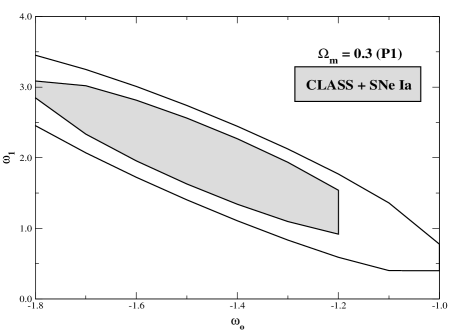
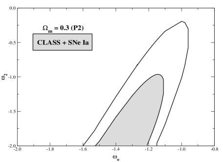
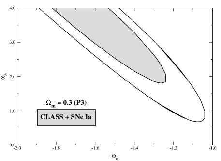
Figure 1: Current constraints on the plane $\omega-\omega_{j}$ from CLASS lensing statistics and SNe Ia data. Note that for the three different parametrizations considered in this paper the joint CLASS + SNe Ia analysis clearly prefers the regions where $\omega_{j}\neq 0$, i.e., a time-dependent EOS. a) Confidence regions (68.3% and 95.4%) in the plane $\omega-\omega_{1}$ for P1. b) The same as in Panel 1a for P2. c) The same as in Panel 1a for P3.

The two large-scale galaxy surveys, namely, the 2dFGRS and the SDSS have produced converging results on the total LF. The surveys determined the Schechter parameters for galaxies (all types) at $z\leq 0.2$. Chae chae1 has worked extensively on the information provided by these recent galaxy surveys to extract the local type-specific LFs. For our analysis here, we adopt the normalization corrected Schechter parameters of the 2dFGRS survey chae1 ; folkes : $\alpha=-0.74$, $\phi^{*}=0.82\times 10^{-2}h^{3}\mathrm{Mpc^{-3}}$, $v^{*}=185\,\mathrm{km/s}$ and $F^{*}=0.014$.

The normalized image angular separation distribution for a source at $z_{S}$ is obtained by integrating $\frac{d^{2}\tau}{dz_{L}\,d\phi}$ over $z_{L}$:

$${d{\mathcal{P}}\over d\phi}\,=\,{1\over\tau(z_{S})}\int_{0}^{z_{s}}\,{\frac{d^{2}\tau}{dz_{L}d\phi}}{dz_{L}}.$$ (12)

The corrected (for magnification and selection effects) image separation distribution function for a single source at redshift $z_{S}$ is given by CSK1

$$P^{\prime}(\Delta\theta)\, = \,\mathcal{B}\,{{{\gamma}}\over 2\,\Delta\theta}\int_{0}^{z_{S}}\left[{D_{OS}\over{D_{LS}}}\phi\right]^{{\frac{\gamma}{2}}(\alpha+1+{\frac{4}{\gamma}})}\,F^{*}\,{cdt\over dz_{L}}$$ (13)

$$\times\exp\left[-\,\left({D_{OS}\over{D_{LS}}}\phi\right)^{\frac{\gamma}{2}}\right]{(1+z_{L})^{3}\over\Gamma\left(\alpha+{4\over\gamma}+1\right)}$$

$$\times\left[\,\left({D_{OL}D_{LS}\over R_{0}D_{OS}}\right)^{2}\,{1\over R_{0}}\right]\,\,{dz_{L}}.$$

Similarly, the corrected lensing probability for a given source at redshift $z$ is given by

$$P^{\prime}=\tau(z_{S})\,\int{d{\mathcal{P}}\over d\phi}\mathcal{B}\;d\phi.$$ (14)

Here $\phi$ and $\Delta\theta$ are related to as $\phi={\frac{\Delta\theta}{8\pi(v^{*}/c)^{2}}}$ and $\mathcal{B}$ is the magnification bias. This is considered because, as is widely known, gravitational lensing causes a magnification of images and this transfers the lensed sources to higher flux density bins. In other words, the lensed sources are over-represented in a flux-limited sample. The magnification bias ${\mathcal{B}}(z_{S},S_{\nu})$ increases the lensing probability significantly in a bin of total flux density ($S_{\nu}$) by a factor

$$\mathcal{B}(z_{S},S_{\nu})\, = \,\left|\frac{dN_{z_{S}}(>S_{\nu})}{dS_{\nu}}\right|^{-1}$$

$$\times\int_{\mu_{min}}^{\mu_{max}}\left|\frac{dN_{z_{S}}(>S_{\nu}/\mu)}{dS_{\nu}}\,p(\mu)\right|{1\over\mu}\,d\mu.$$

In the above expression, $N_{z_{S}}(>S_{\nu})$ is the intrinsic flux density relation for the source population at redshift $z_{S}$. $N_{z_{S}}(>S_{\nu})$ gives the number of sources at redshift $z_{S}$ having flux greater than $S_{\nu}$. For the SIS model, the magnification probability distribution is $p(\mu)=8/{\mu}^{3}$. The minimum and maximum total magnifications $\mu_{min}$ and $\mu_{max}$ in equation (III.1) depend on the observational characteristics as well as on the lens model. For the SIS model, the minimum total magnification is $\mu_{min}\simeq 2$ and the maximum total magnification is $\mu_{max}=\infty$. The magnification bias $\mathcal{B}$ depends on the differential number-flux density relation $\left|dN_{z_{S}}(>S_{\nu})/dS_{\nu}\right|$. The differential number-flux relation needs to be known as a function of the source redshift. At present redshifts of only a few CLASS sources are known. We, therefore, ignore redshift dependence of the differential number-flux density relation. Following Chae chae1 , we further ignore the dependence of the differential number-flux density relation on the spectral index of the source.

Two important selection criteria for CLASS statistical sample are (i) that the ratio of the flux densities of the fainter to the brighter images ${\mathcal{R}}_{min}$ is $\geq 0.1$. Given such an observational limit, the minimum total magnification for double imaging the adopted model of the lens is $\mu_{min}=2(1+\mathcal{R}_{min}/1-\mathcal{R}_{min})$ chae1 ; (ii) that the image components in lens systems must have separations $\geq 0.3$ arcsec. We incorporate this selection criterion by setting the lower limit of $\Delta\theta$ in equation (14) as $0.3$ arcsec.

III.2 SNe Ia sample.

The SNe Ia sample of Riess et al. rnew consists of 186 events distributed over the redshift interval $0.01\lesssim z\lesssim 1.7$ and constitutes the compilation of the best observations made so far by the two supernova search teams plus 16 new events observed by HST. This total data-set was divided into “high-confidence” (gold) and “likely but not certain” (silver) subsets. Here, we will consider only the 157 events that constitute the so-called gold sample. The best fit to the set of parameters $\mathbf{s}$ is obtained by using a $\chi^{2}$ statistics, i.e.,

$$\chi^{2}_{SNe}=\sum_{i=1}^{157}{\frac{\left[\mu_{p}(z|\mathbf{s})-\mu_{o}^{i}(z|\mathbf{s})\right]^{2}}{\sigma_{i}^{2}}},$$ (16)

where $\mu_{p}(z|\mathbf{s})=m-M=5\mbox{log}d_{L}+25$ is the predicted distance modulus for a supernova at redshift $z$, $\mu_{o}^{i}(z|\mathbf{s})$ is the extinction corrected distance modulus for a given SNe Ia at $z_{i}$, and $\sigma_{i}$ is the uncertainty in the individual distance moduli, which includes uncertainties in galaxy redshift due to a peculiar velocity of 400 km/s. The Hubble parameter $H_{o}$ is considered a “nuisance” parameter so that we marginalize over it (For some recent SNe Ia studies, see sne ).

III.3 Results.

The main results of our joint analysis are displayed in Figure 1. Panels 1a-1c show the confidence regions ($68.3\%$ and $95.4\%$) in the $\omega_{o}-\omega_{j}$ plane for P1, P2 and P3, respectively. As stated earlier, the matter density parameter has been fixed in all analyses at $\Omega_{m}=0.3$, in agreement with some clustering estimates calb . The contours are defined by the conventional two-parameter $\chi^{2}$ levels (2.30 and 6.17), where $\chi^{2}_{total}=\chi^{2}_{SNe}-2{\rm{ln}}l$ and $l={\cal{L}}_{lens}/{\cal{L}}_{max}^{lens}$ is the normalized likelihood for lenses. From this combination of observational data we find that the best-fit parameters for P1 are $\omega_{o}=-1.5$ and $\omega_{1}=2.1$, which corresponds to an accelerating scenario with transition redshift (at which the Universe switches from acceleration to acceleration) $z_{t}\simeq 0.26$ and a total expanding age of $\simeq 7.0h^{-1}$ Gyr. For parametrizations 2 and 3 the best-fit scenarios occur at $\omega_{o}=-1.4$ and $\omega_{2}=-2$ and $\omega_{o}=-1.7$ and $\omega_{3}=4.1$, corresponding to a $10h^{-1}$-Gyr-old and $7.5h^{-1}$-Gyr-old universes with transition redshifts at $z_{t}\simeq 0.53$ and $z_{t}\simeq 0.31$, respectively. Note that the estimates of $z_{t}$ for P2 and P3 are inside the 1$\sigma$ interval inferred for the transition redshift from the current SNe Ia data rnew (see also daly ). The best-fit values for each parametrization also imply a beginning of a phantom behavior at $z_{ph}\simeq 0.23$ (P1), $z_{ph}\simeq 0.22$ (P2) and $z_{ph}\simeq 0.20$ (P3).

From the above figures, however, it is clear the most important conclusion one may reach resides on the fact that for the three parametrizations considered in this paper the joint CLASS + SNe Ia analysis clearly prefers the regions where $\omega_{j}\neq 0$, i.e., a time-dependent EOS. In particular, note that the point $\omega_{j}=0$, which means a time-independent EOS, is at least 2$\sigma$ off from the central values obtained for this parameter. Such a result seems to be more restrictive than that obtained in Ref. teg (see also padn ), in which a combination of the latest SNe Ia, cosmic microwave background and large-scale structure data showed no hint of departures from the model corresponding to Einstein’s cosmological constant ($\omega_{j}=0$ and $\omega_{o}=-1$). It is possible that this particular preference for a time-dependent EOS changes if the current cosmic microwave background (CMB) data were included in the analysis. As discussed in padn , an evolving dark energy EOS affects the features of temperature anisotropies in CMB in at least two ways, namely, the position of the acoustic peaks as well as the integrated Sachs-Wolf efect. However, if independent analyses involving a more significant number of different data sets confirm this preference of the observational data for values of $\omega_{j}\neq 0$, these results surely will bring to light a new consistency problem for our current standard cosmological model since for this case $\omega_{j}$ is necessarily null.

IV Conclusion

Very recently, the field of cosmology has entered a golden era. An era where new and revolutionary concepts were introduced with the support of a plethora of high-quality observational data. Surely, the most remarkable among these concepts is the idea of a dark energy-dominated universe, which is motivated from an impressive convergence of independent observational results. This idea in turn gave rise to the so-called dark energy problem since the nature of this dark component is completely unknown at present.

In this paper, although aware of the impossibility of determining the nature of the dark energy on the basis only of observational data, we have considered the possibility of discriminating two of our favorite candidates for this mysterious component, namely, the cosmological constant ($\Lambda$) and a dynamical scalar field ($\phi$) [33]. By considering three different parametrizations for the dark enegy EOS, we have placed limits on the time-dependent term of these parametrizations ($\omega_{j}$) from a joint analysis involving the most recent radio sources gravitational lensing sample and SNe Ia data. We have shown that this particular combination of observational data prefer values of $\omega_{j}\neq 0$, i.e., a time-dependent EOS. We believe that if such a result is confirmed by the upcoming observations, it may shed some light on our search for a better understanding of the nature of the so-called dark energy.

- (1) M. S. Turner and M. White, Phys. Rev. D56, R4439 (1997); R. R. Caldwell, Phys. Lett. B545, 23 (2002); M. C. Bento, O. Bertolami and A. A. Sen, Phys. Rev. D66, 043507 (2002); A. Dev, D. Jain and J. S. Alcaniz, Phys. Rev. D67, 023515 (2003). astro-ph/0209379; J. S. Alcaniz, D. Jain and A. Dev, Phys.Rev. D67, 043514 (2003). astro-ph/0210476; J. S. Alcaniz, Phys. Rev. D69, 083521 (2004). astro-ph/0312424. Z.-H. Zhu, M.-K. Fujimoto and X.-T. He, Astron. Astrophys. 417, 833 (2004); H. Stefancic, Phys. Rev. D71, 084024 (2005); O. Bertolami and P. T. Silva, astro-ph/0507192; Z-K Guo, Y-S Piao,X-M Zhang and Y-Z Zhang, Phys. Lett. B608, 177 (2005).
- (2) V. Sahni and Y. Shtanov, IJMP D11, 1515 (2002); JCAP 0311, 014 (2003); C. Deffayet, G. Dvali and G. Gabadadze, Phys. Rev. D65, 044023 (2002); J. S. Alcaniz, Phys. Rev. D 65, 123514 (2002). astro-ph/0202492; M. D. Maia et al., Class. Quant. Grav. 22, 1623 (2005). astro-ph/0403072.
- (3) J. A. S. Lima and J. S. Alcaniz, Phys. Lett. B600, 191 (2004). astro-ph/0402265 (2004); P. F. Gonzalez-Diaz and C. L. Siguenza, Nucl. Phys. B697, 363 (2004). astro-ph/0407421. I. Brevik, S. Nojiri, S. D. Odintsov and L. Vanzo, Phys. Rev. D70, 043520 (2004). hep-th/0401073
- (4) J. Kratochvil, A. Linde, E. V. Linder and M. Shmakova, JCAP 0407 001 (2004)
- (5) C. Deffayet et al., Phys. Rev. D66, 024019 (2002)
- (6) K. -H. Chae et al., Phys. Rev. Lett., 89, 151301 (2002)
- (7) A. G. Riess et al., Astrophys. J. 607, 665 (2004)
- (8) A. R. Cooray and D. Huterer, Astrophys. J. 513, L95 (1999)
- (9) I. Waga and A. P. M. R. Miceli, Phys. Rev D59, 103507 (1999); P. T. Silva and O. Bertolami, Astrophys. J. 599 829 (2003)
- (10) A. Dev, D. Jain and J. S. Alcaniz, Astron. Astrophys. 417, 847 (2004)
- (11) P. Astier, astro-ph/0008306; J. Weller and A. Albrecht, Phys. Rev D65, 103512 (2002); I. Maor et al., Phys. Rev D65, 123003 (2002)
- (12) M. Goliath et al., Astron. Astrophys. 380, 6 (2001)
- (13) A. C. S. Friaça, J. S. Alcaniz and J. A. S. Lima, Submitted to Mon. Not. Roy. Astron. Soc. (2004)
- (14) G. Efstathiou, Mon. Not. Roy. Astron. Soc., 310, 842 (1999)
- (15) M. Chevallier and D. Polarski, Int. J. Mod. Phys. D10, 213 (2001); gr-qc/0009008
- (16) E. V. Linder, Phys. Rev. Lett. 90, 091301 (2003)
- (17) T. Padmanabhan and T. Roy Choudhury, Mon. Not. Roy. Astron. Soc. 344, 823 (2003)
- (18) Y. Wang and P. M. Garnavich, Astrophys. J. 552 445 (2001); C. R. Watson and R. J. Scherrer, Phys. Rev. D68, 123524 (2003); P.S. Corasaniti et al., Phys. Rev. D70, 083006 (2004); V. B. Johri, astro-ph/0409161
- (19) Y. Wang and M. Tegmark, Phys. Rev. Lett. 92, 241302-1 (2004)
- (20) H. K. Jassal, J. S. Bagla, and T. Padmanabhan, Mon. Not. Roy. Astron. Soc. 356, L11 (2005). astro-ph/0404378.
- (21) R. G. Calberg et al., Astrophys. J. 462, 32 (1996)
- (22) K. -H. Chae 2002, (astro-ph/0211244)
- (23) A. Dev, D. Jain and S. Mahajan, Int. J. Mod. Phys. D13, 1005 (2004). astro-ph/0307441
- (24) I. W. A. Browne et al. 2002, Mon. Not. Roy. Astron. Soc. 341, 13 (2003)
- (25) E. L. Turner, J. P. Ostriker and J. R, Gott, Astrophys. J. , 284, 1 (1984)
- (26) P. L. Schechter, Astrophys. J. 203, 297 (1976)
- (27) M. Fukugita, T. Futamase and M. Kasai, MNRAS, 246, 24 (1990); E. L. Turner, Astrophys. J. , 365, L43 (1990); M. Fukugita, T. Futamase, M. Kasai and E. L. Turner, Astrophys. J. , 393, 3 (1992)
- (28) S. Folkes et al., Mon. Not. Roy. Astron. Soc., 308, 459 (1999)
- (29) S. M. Faber and R. E. Jackson, Astrophys. J. , 204, 668 (1976)
- (30) C. S. Kochanek, Astrophys. J. , 466, 638 (1996); M. Chiba and Y. Yoshii, Astrophys. J. 510, 42 (2001)
- (31) T. R. Choudhury and T. Padmanabhan, Astron. Astrophys. 429, 807 (2005). astro-ph/0311622; S. Nesseris and L. Perivolaropoulos, Phys. Rev D70, 043531 (2004). astro-ph/0401556; O. Bertolami, A. A. Sen, S. Sen and P. T. Silva, astro-ph/0402387; J. S. Alcaniz and N. Pires, Phys. Rev D70, 047303 (2004). astro-ph/0404146; Z.-H. Zhu and M.-K. Fujimoto, Astrophys. J. 585, 52 (2003); M. C. Bento, O. Bertolami, N. M. C. Santos and A. A. Sen, Phys. Rev. D71, 063501 (2005), astro-ph/0412638; J.S. Alcaniz and Z-H Zhu, Rev. D71, 083513 (2005). astro-ph/0411604.
- (32) R. A. Daly and S. G. Djorgovski, astro-ph/0403664 (2004); U. Alam, V. Sahni and A. A. Starobinsky, J. Cosm. Astrop. Phys. 0406, 008 (2004). astro-ph/0403687 (2004)