Can Virialization Shocks be Detected Around Galaxy Clusters
Through the Sunyaev-Zel’dovich Effect?

Abstract

In cosmological structure formation models, massive non–linear objects in the process of formation, such as galaxy clusters, are surrounded by large-scale shocks at or around the expected virial radius. Direct observational evidence for such virial shocks is currently lacking, but we show here that their presence can be inferred from future, high resolution, high–sensitivity observations of the Sunyaev-Zel’dovich (SZ) effect in galaxy clusters. We study the detectability of virial shocks in mock SZ maps, using simple models of cluster structure (gas density and temperature distributions) and noise (background and foreground galaxy clusters projected along the line of sight, as well as the cosmic microwave background anisotropies). We find that at an angular resolution of $2^{\prime\prime}$ and sensitivity of $10\mu\mathrm{K}$, expected to be reached at $\sim 100$ GHz frequencies in a $\sim 20$hr integration with the forthcoming ALMA instrument, virial shocks associated with massive ($M\sim 10^{15}~{}{\rm M_{\odot}}$) clusters will stand out from the noise, and can be detected at high significance. More generally, our results imply that the projected SZ surface brightness profile in future, high–resolution experiments will provide sensitive constraints on the density profile of cluster gas.

1. Introduction

In cosmological theories of structure formation, non–linear objects form when overdense dark matter perturbations turn around, collapse, and settle into virial equilibrium (e.g. Peebles 1993 and references therein). Gas initially collapses together with the dark matter, but eventually encounters nearly stationary material that had already collapsed. Since the gas is falling in at supersonic velocities, it is slowed down by hydrodynamical shocks, and these shocks are thought to heat the gas to the virial temperature of the dark matter halo.

In spherically symmetric models, and in the absence of dissipation, a single strong gaseous shock occurs at approximately half of the turn–around radius (Bertschinger, 1985), coinciding with the “virial radius” of the dark matter halo. More realistically, the behavior of the post–shock gas depends sensitively on its cooling time (Rees & Ostriker, 1977). On galactic scales ($M\sim 10^{12}~{}{\rm M_{\odot}}$) and below, and increasingly toward high redshifts ($z\mathrel{\hbox to0.0pt{\lower 4.0pt\hbox{\hskip 1.0pt$\sim$}\hss}\raise 1.0pt\hbox{$>$}}3$), the gas can cool rapidly and loose its pressure support, and hence continue its infall. On these scales, the existence of large–scale shocks have been recently called into question by models in which the bulk of the infalling gas remains cold, and reaches the central regions of the dark halo before encountering shocks (Birnboim & Dekel, 2003; Keres et al., 2004). On larger scales, however, where cooling times are long, such as for galaxy clusters, the existence of virial shocks remains an unambiguous prediction of cosmological structure formation theories. Detailed three–dimensional hydrodynamical simulations of cluster formation (e.g. Evrard 1990; Bryan & Norman 1998) have confirmed the existence of virial shocks, with strong discontinuities in gas density and temperature. These and subsequent simulations have also revealed that the infall is anisotropic, with gas falling in to the cluster potential along cosmic filaments. As a result, the radial location and strength of the shocks varies along different directions.

The virial shocks are a fundamental ingredient of cosmic structure formation, and may be responsible for diverse phenomenae, such as generating large–scale cosmic magnetic fields (Bagchi et al., 2002) and accelerating electrons to contribute to the diffuse cosmic gamma–ray background (Loeb & Waxman, 2000). The radial location of the shocks, in principle, also contains information on the cosmological parameters (Verde et al., 2002). Despite their importance, direct evidence for the existence of such shocks does not yet exist. The major difficulty in observing the virial shock is that it is expected to lie several Mpc (and several arcminutes) away from the cluster center, a location at which signals such as the X–ray surface brightness (Tozzi et al., 2000), or galaxy number density/peculiar velocities (which could reveal density caustics, Rines et al. 2003) diminish rapidly.

In this paper, we consider the detectability of virial shocks in future observations of galaxy clusters through the Sunyaev-Zel’dovich (SZ) effect. The thermal SZ effect is a secondary distortion of the cosmic microwave background (CMB) spectrum caused by the hot intra–cluster gas along the line of sight to the surface of last scattering (see Sunyaev & Zeldovich 1980 for a review). The cool CMB photons undergo inverse Compton scattering on the hot electrons, gaining on average a small amount of energy in the process, creating an intensity decrement at low frequencies ($\nu\lesssim 218\mathrm{GHz}$) and an increment at high frequencies. The SZ effect is the dominant source of CMB anisotropy at small angular scales.

The SZ effect has recently become a valuable observational tool (Birkinshaw, 1999). Several programs have begun to map out massive clusters of galaxies, study the intracluster medium (ICM), and constrain cosmological parameters. Current instruments are now detecting and imaging clusters at high signal-to-noise, and the next generation of instruments should be capable of mapping significant portions of the sky as a means of finding clusters of galaxies (see Carlstrom et al. 2002 for a review). Several studies have predicted the number of clusters that could be detected in future SZ surveys (Bartlett, 2001; Holder et al., 2000; Haiman et al., 2001; Barbosa et al., 1996; Kneissl et al., 2001). The survey yields are quite impressive. Next generation instruments, such as the Atacama Cosmology Telescope (ACT), South Pole Telescope (SPT), and the Planck satellite, are expected to detect several clusters per day; the large resulting samples can be used to select the most massive and most regular clusters that will be best suited for the studies proposed here.

The SZ effect is ideally suited to study the “outskirts” of clusters, because the SZ temperature decrement profile is relatively flat (e.g. $\Delta T\propto\rho$, whereas the X–ray emission is proportional to the square of the local density; Komatsu & Seljak (2001)). Although our main focus is to assess the significance at which the shocks can be detected, we also consider the more general problem of constraining the cluster gas distribution, as well as the structure of the dark matter halos themselves.

The detection of sharp features, such as the virial shocks, calls for high sensitivity, high–resolution maps of the SZ surface brightness profile of the most massive clusters. For this reason, we here focus on predictions appropriate for the Atacama Large Millimeter Array (ALMA), a telescope array expected to be operational in 2012 and deliver $\sim$arcsecond resolution, high–sensitivity imaging of clusters. Our results can be scaled to apply to other instruments with different parameters.

This paper is organized as follows. In § 2, we summarize the relevant characteristics of ALMA. In § 3, we describe our models for the structure of galaxy clusters. These models are based on standard descriptions of gas in hydrostatic equilibrium with a dark matter halo, except that we introduce additional free parameters that allow us to vary the location and sharpness of the ’virial shock. In § 4, we compute and contrast the SZ surface brightness profiles in models with different virial shocks. In § 5, we discuss the sources of noise in the SZ surface brightness maps. In § 6, we present simple estimates to argue that, in the face of noise, smooth cluster profiles can be distinguished at high significance from profiles that include a virial shock. In § 7, we go one step further, and compute the statistical accuracy at which the location and sharpness of the shock fronts, as well as other parameters describing the cluster profile, can be determined from future SZ maps. Finally, in § 8 we summarize our conclusions and discuss the implications of this work. Several technical points, related to our statistical analysis, are discussed in the Appendices.

Throughout this paper we assume a standard cold–dark matter cosmology ($\Lambda$CDM), with ($\Omega_{\Lambda}$, $\Omega_{M}$, $\Omega_{b}$, $H_{0}$) = (0.7, 0.3, 0.045, 70 km s^-1 Mpc^-1), consistent with the recent results from WMAP (Spergel et al., 2003).

2. ALMA

The three crucial characteristics of any instrument for the detection of the virial shocks are angular resolution (needed since the features caused by the shocks are sharp), angular coverage (needed since the features can extend coherently over arcminute scales), and sensitivity (the surface brightness change across the shock–front is as small as a few $\mu$K). ALMA has an ideal combination of these three qualities, and is well suited to studying the gas density cutoff. ALMA will be comprised of sixty four 12-meter sub-millimeter quality antennae, with baselines extending from 150 m up to 10 km. Its receivers will cover the range from $\nu=70$ to $900$ GHz. Anticipated SZ temperature sensitivity for a $\Delta t_{s}\approx 60s$ integration period is between $\sigma_{D}\approx 100\mu\mathrm{K}$ and $24$mK for the compact configuration depending on the frequency of the detection.

The expected aperture efficiency of an antenna has been taken from Butler et al. (1999). Generally, a baseline $B$ corresponds to a beam radius

$$\Delta\phi=\frac{c}{\nu B}=2"\times\left(\frac{\nu}{100\mathrm{GHz}}\right)^{-1}\left(\frac{B}{300\mathrm{m}}\right)^{-1}.$$ (1)

The resulting temperature sensitivities for the compact configuration ($B=150\mathrm{m}$) is given in Table 1. In our calculations below, we will assume a frequency of 100 GHz, but Table 1 shows the required integration time and baseline for several different frequencies. The second and third columns show the beam diameter and the sensitivity at a fixed integration time of 60s. In the fourth and fifth columns, we calculated the baseline needed to have $\Delta\phi\leq 2"$ and the corresponding sensitivity at the same fixed integration time of $60s$. In the last column we calculated the integration time $\Delta t_{\rm int}$ needed to reduce the r.m.s. noise variance to $10\mu\mathrm{K}$ (using the scaling $\sigma_{D}\propto\sqrt{B^{2}\Delta t_{\rm int}}$).

Table 1Temperature sensitivities and integration times

$\nu$	$\phi$	$(\sigma_{D})_{60s}$	$B$	$(\sigma_{D})_{60s}$	$(\Delta t_{\rm int})_{10\mu\mathrm{K}}$
[GHz]	[arcsec]	[mK]	[m]	[mK]	[hr]
35	11.79	0.1079	884	3.747	67
90	4.584	0.1871	344	0.983	31
140	2.947	0.2518	221	0.547	23
230	1.794	0.4317	150	0.432	31
345	1.196	1.007	150	1.007	169
409	1.009	1.799	150	1.799	539
650	0.6347	13.67	150	13.67	$3.11\times 10^{4}$
850	0.4853	24.46	150	24.46	$9.97\times 10^{4}$

For the present study we will assume that the sensitivity of the detector is $\sigma_{D}\lesssim 10\mu$K, and its angular resolution is $\Delta\phi\approx 2"$. As Table 1 shows, these assumptions are realistic for ALMA, requiring $23-170$ hr integration for all frequencies below $350\mathrm{GHz}$. For even longer observation times, the detector noise can be neglected compared to the statistical fluctuations of astrophysical origin (the latter, which has a magnitude of $\sim 10\mu$K, will be discussed in § 5 below).

3. Self-Similar Cluster Density and Temperature Profiles

In this section, we describe the models we adopt for the density and temperature profiles of gas in the cluster. These models assume that clusters are described by spherically symmetric dark matter halos. We first follow Komatsu & Seljak (2001) to obtain self–similar gas density and temperature profiles. These profiles are then truncated and normalized according to the assumed location and sharpness of a virial shock.

Many high-resolution N-body simulations suggest that the dark matter density profile $\rho_{\mathrm{dm}}(r)$ is well described by a self–similar form: $\rho_{\mathrm{dm}}(r)=\rho_{s}y_{\mathrm{dm}}(r/r_{s})$ where $\rho_{s}$ is the mass density normalization factor, $r_{s}$ is a length scale, and $y_{\mathrm{dm}}(x)$ is a non-dimensional function representing the profile. The density normalization, $\rho_{s}$, is determined to yield mass $M_{\mathrm{vir}}$ when $\rho_{\mathrm{dm}}(r)$ is integrated within the virial radius, $r_{\mathrm{vir}}$. The length scale $r_{s}$ is defined as $r_{s}=r_{\mathrm{vir}}/c$, where $c$ is the concentration parameter. We use a fitting formula from detailed gas dynamical simulations for the concentration parameter (see eq. 12 below), and calculate $r_{\mathrm{vir}}(M_{\mathrm{vir}},z)$ from the top–hat collapse model (see discussion below).

The dark-matter profile is approximated by the following analytic form

$$y_{\mathrm{dm}}(x)=\frac{1}{x^{\alpha}(1+x)^{3-\alpha}},$$ (2)

where the parameter $\alpha$ is assumed to be either $\alpha=1$ or $\alpha=3/2$ (see Navarro et al. 1997, Moore et al. 1999, and Jing & Suto 2000).

The gas density profile can be obtained using a polytropic model in hydrostatic equilibrium with the dark matter background. In this case, the gas density and temperature profiles assume a self–similar form,

$$\rho_{\mathrm{gas}}(r/r_{s}) =\rho_{\mathrm{gas}}(0)y_{\mathrm{gas}}(r/r_{s})$$ (3)

$$T_{\mathrm{gas}}(r/r_{s}) =T_{\mathrm{gas}}(0)y_{\mathrm{gas}}^{\gamma-1}(r/r_{s}),$$ (4)

where $P_{\mathrm{gas}}\propto\rho_{\mathrm{gas}}T_{\mathrm{gas}}\propto\rho^{\gamma}$ has been used. The hydrostatic equilibrium equation

$$\rho_{\mathrm{gas}}^{-1}\frac{\mathrm{d}P_{\mathrm{gas}}}{\mathrm{d}r}=-G\frac{M(\leq r)}{r^{2}}$$ (5)

can be solved (Suto et al., 1998) for $y_{\mathrm{gas}}(x)$ for a fixed dark matter mass distribution.

$$y_{\mathrm{gas}}^{\gamma-1}(x)=1-3\eta^{-1}\frac{\gamma-1}{\gamma}\frac{c}{m(c)}\int_{0}^{x}\mathrm{d}u\frac{m(u)}{u^{2}},$$ (6)

where $\eta$ is an integration constant, $x$ is defined as

$$x=\frac{r}{r_{s}},$$ (7)

and $m(u)$ is the dimensionless mass within a distance $u$ from the center

$$m(x)\approx m_{\mathrm{dm}}(x)=4\pi\int_{0}^{x}\mathrm{d}uu^{2}y_{\mathrm{dm}}(u).$$ (8)

These integrals can be evaluated analytically (Suto et al., 1998) for the particular cases $\alpha=1$ and $\alpha=3/2$.

The mass-temperature normalization is given by the virial theorem

$$\eta^{-1}=\frac{G\mu m_{\mathrm{p}}M_{\mathrm{vir}}}{3r_{\mathrm{vir}}k_{\mathrm{B}}T_{\mathrm{gas}}(0)}.$$ (9)

Both theoretical and numerical studies assert that the gas density profile traces the dark matter density profile in the outer regions of the halo. Therefore, the slopes of these two profiles are assumed to track each other closely for $c/2<x<2c$. This requirement fixes the polytropic index $\gamma$, and the normalization $\eta$ (see equations 22, 23, and 25 in Komatsu & Seljak 2001).

The concentration parameters, $c$ and $c_{NFW}$ can be written in terms of the virial mass and redshift for a given cosmological model. A fitting formula based on numerical simulations (Eke et al., 2001) is

$$c(M_{\mathrm{vir}},\alpha,z) =\left\{\begin{array}[]{c}c_{NFW}\text{~{}if~{}~{}}\alpha=1\\ c_{NFW}/1.7\text{~{}if~{}~{}}\alpha=1.5\\ \end{array}\right.$$ (12)

$$c_{NFW} =\frac{6}{1+z}\left(\frac{M_{\mathrm{vir}}}{10^{14}h^{-1}M_{\odot}}\right)^{-1/5}.$$ (13)

Equation (12) supplies a one–to–one correspondence between $c$ and $M_{\mathrm{vir}}$.

The self–similar model defined above does not assign a value for the gas density normalization $\rho_{\mathrm{gas}}(0)$. Its value can be calculated by requiring that the ratio of the total dark matter and gas mass within some radius $x_{\mathrm{max}}$ attain the universal average value of $\Omega_{\mathrm{dm}}/\Omega_{\mathrm{B}}$. Simulations without feedback from galaxy formation typically find values for the cluster gas mass fraction that are only slightly lower than the input global baryon fraction (Evrard, 1997). Using cosmological parameters cited above

$$\rho_{\mathrm{gas}}(0)=\rho_{s}\frac{m_{\mathrm{dm}}(x_{\mathrm{max}})}{m_{\mathrm{gas}}(x_{\mathrm{max}})}\frac{\Omega_{\mathrm{B}}}{\Omega_{\mathrm{dm}}},$$ (14)

where $m_{\mathrm{gas}}(x)$ is the accumulated dimensionless mass of the gas analogous to $m_{\mathrm{dm}}(x)$ defined in equation (8). The parameter $\rho_{\mathrm{gas}}(0)$ has only a mild $x_{\mathrm{max}}$ dependence for reasonably low $x_{\mathrm{max}}$ values. Using a fixed $x_{\mathrm{max}}=5c$ yields a maximum error of 10% for $x_{\mathrm{max}}\in[c,10c]$.

We calculate the virial radius, $r_{\mathrm{vir}}$, using the spherical top hat collapse model, i.e. we take it to be the radius of a spherical region with mean interior overdensity $\Delta_{c}$ relative the critical (obtained from the fitting formula in equation 6 of Bryan & Norman 1998) that encloses a total mass $M_{\rm vir}$. The corresponding angular radius of the cluster is

$$\Theta_{\mathrm{vir}}=\frac{r_{\mathrm{vir}}}{d_{A}(z)}=r_{\mathrm{vir}}\frac{(1+z)^{2}}{d_{L}(z)},$$ (15)

where we adopt a fitting formula (Pen, 1999) for $d_{L}(z)$. With this choice, the only free parameters needed to specify the full gas density profile, $\rho_{\mathrm{gas}}(r)$, are $M_{\mathrm{vir}}$, $\alpha$, and $z$.

Let us now introduce a truncation of the density (and temperature) profile (2) to account for the shock front near the virial radius of the cluster. As pointed out above (see eq. 14), such a truncation was already needed for calculating the normalization of the gas density. Let us assume that the density has a linear cutoff between radii $x_{\mathrm{max}}-D$ and $x_{\mathrm{max}}+D$. At $x_{\mathrm{max}}+D$ the density attains the background value. Since this value is small compared to $y_{\mathrm{dm}}(c)$ for realistic clusters, we set both the gas density and temperature at $x>x_{\mathrm{max}}+D$ to zero. Since the gas density profile traces the dark matter profile, the linear density cutoff can be imposed directly on the gas density. In what follows, we will refer to the original density profile (eq. 6) as ${y_{\mathrm{gas}}}_{0}(x)$. We will denote the density profile with a cutoff by $y_{\mathrm{gas}}(x)$, defined by

$$y_{\mathrm{gas}}(x)={y_{\mathrm{gas}}}_{0}(x)W(x),$$ (16)

where

$$W(x)=\left\{\begin{array}[]{lll}1&\text{if~{}~{}}x<x_{\mathrm{max}}-D\\ {[(x_{\mathrm{max}}+D)-x]}/{(2D)}&\text{if~{}~{}}x_{\mathrm{max}}+D<x<x_{\mathrm{max}}-D\\ 0&\text{if~{}~{}}x_{\mathrm{max}}+D<x\\ \end{array}\right.$$ (17)

For consistency, the $\rho_{\mathrm{gas}}(0)$ gas density normalization has to be recalculated from equation (14) using the mass $m(x)$ enclosed by the density profiles truncated with a given choice of $x_{\mathrm{max}}$ and $D$ (see eq. 8). In practice, $\rho_{\mathrm{gas}}(0)$ is sensitive to $x_{\mathrm{max}}$ only, with the $D$ dependence nearly negligible. Thus, for calculating the normalization $\rho_{\mathrm{gas}}(0)$, we always assume $D=0$ in equation (14).

4. SZ surface brightness profiles

The two–dimensional SZE intensity profile $I(x)$, as a function of projected radial distance $x$ away from the cluster center, is often expressed as a small temperature change of the CMB spectrum. The SZE corresponding temperature increment $\Delta T(x)$ (which can be negative) is defined by

$$I(x)=\frac{\partial I_{CMB}}{\partial T_{CMB}}\Delta T(x).$$ (18)

Solving for the SZE temperature yields (Carlstrom et al., 2002)

$$\Delta T(x)=f(\theta)y_{C}(x)T_{CMB},$$ (19)

where $\theta={h\nu}/{k_{\mathrm{B}}T_{\mathrm{CMB}}}$ is the dimensionless frequency, $y_{C}$ is the Compton parameter, and $f(\theta)$ is given by

$$f(\theta)=\left(\theta\frac{e^{\theta}+1}{e^{\theta}-1}-4\right)(1+\delta_{SZE}(\theta,T_{e})).$$ (20)

The $\delta_{SZE}(x,T_{e})$ term is the relativistic correction to the frequency dependence, which is negligible at 100 GHz, but becomes important at higher frequencies ($\mathrel{\hbox to0.0pt{\lower 4.0pt\hbox{\hskip 1.0pt$\sim$}\hss}\raise 1.0pt\hbox{$>$}}250$ GHz). The Compton $y_{C}$-parameter is defined as

$$y_{C}(x)=\frac{k_{B}\sigma_{T}}{m_{e}c^{2}}\int n_{e}T_{e}\mathrm{d}l$$ (21)

where $\sigma_{T}$ is the Thompson cross-section, $n_{e}$ is the electron number density, $T_{e}$ is the electron temperature, $k_{B}$ is the Boltzmann constant, $m_{e}c^{2}$ is the electron rest mass energy, and the integration is along the line of sight (i.e. along $r=\sqrt{x^{2}+l^{2}}$ for a given $x$). We calculate the electron temperature, $T_{e}$, with $T_{e}=T_{\mathrm{gas}}$ using equation (9), and the number density is given by

$$n_{e}(x)=\frac{\rho_{\mathrm{gas}}(0)y_{\mathrm{gas}}(x)}{\mu m_{\mathrm{p}}}$$ (22)

where $m_{\mathrm{p}}$ is the proton rest mass, and $\mu=0.59$ for an ionized H-He plasma with $25\%$ Helium abundance by mass.

Figure 1.— Predicted SZ surface brightness profiles for $M_{\mathrm{vir}}=10^{15}M_{\odot}$, $z=0.1$, $\alpha=1.5$, and $\nu=100\mathrm{Hz}$. The solid curve shows the profile without a cutoff (the calculation used $x_{\mathrm{max}}=200$ and $D=0$ in practice), and the dotted line corresponds to the SZ profile with $x_{\mathrm{max}}=c$ and $D=0$. Equation (23) was evaluated with $\Delta T(0)=0.7\mathrm{mK}$.

Substituting (4), (9), and (22) in (21) the SZ surface brightness profile (19) is separable into a dimensionless integral with spatial dependence and a constant coefficient

$$\Delta T(x)=\Delta T_{s}Y(x),$$ (23)

where

$$\Delta T_{s}=f(\theta)T_{CMB}\sigma_{T}\frac{1}{m_{e}c^{2}}\frac{GM_{\mathrm{vir}}}{3c}\rho_{\mathrm{gas}}(0)\eta$$ (24)

and

$$Y(x)=2\int^{\sqrt{(x_{\mathrm{max}}+D)^{2}-x^{2}}}_{0}\mathrm{d}l\,[y_{\mathrm{gas}}(\sqrt{x^{2}+l^{2}})]^{\gamma}.$$ (25)

Figure 2.— The difference between the normalized brightness profiles with and without a cutoff, for various $D$ values. The difference is taken between the $\Delta T(x)$ profiles with different $x_{\mathrm{max}}$ and $D$ parameters, but identical $(M_{\mathrm{vir}},\alpha,z)=(10^{15}M_{\odot},1.5,0.1)$, and $\Delta T_{s}$ values. The SZ profiles with $x_{\mathrm{max}}=2c$ and $D=0$, $0.2c$, and $0.4c$ were compared with the same profile without a cutoff, for which $x_{\mathrm{max}}=200$ and $D=0$ was used in practice. The fact that $\Delta T-\Delta T^{\rm fid}$ is nonzero at $x=0$ is a consequence of the $x_{\mathrm{max}}$ dependence of Y(x).

Figure 1 depicts the $\Delta T(x)$ profile for $\alpha=1.5$ with and without a cutoff. Without the cutoff, the $y_{\mathrm{gas}}(x)$ and $\Delta T(x)$ profile has a nonzero limit for large $x$. Various choices of $x_{\mathrm{max}}$ can be compared by analyzing the difference between the associated intensity profiles. Figure 2 shows the difference between pairs of profiles with $x_{\mathrm{max}}=2c$ and without a cutoff, using either $D=0$, $0.2c$, or $0.4c$ for the truncated profile. All other parameters, such as $M_{\mathrm{vir}}$, $\alpha$, $z$, and $\Delta T_{s}$ were taken to be equal. Note that the $\Delta T(x)$ profile is obtained from $Y(x)$ by multiplying by the $\Delta T_{s}$ coefficient. According to equation (14), various $x_{\mathrm{max}}$ choices generally lead to unequal $\Delta T_{s}$ values, implying a large nonzero difference between the $\Delta T(x)$ profiles at $x=0$. In principle, this difference is physical, reflecting the normalization criterion we chose (namely that the clusters contain the average baryon fraction within the virial shock – no mechanism is known to segregate baryons from dark matter on these large scales). Since the normalization is model–dependent, one might worry that it will effect our analysis below, where we study the detectability of the virial shocks. However, we find that the information from the normalization does not dominate our results (see discussion below).

Table 2 shows the central $\Delta T(0)$ values for several different cluster masses and density profile slopes, and for various frequencies. We find that the $\alpha=1.5$ dark matter profile yields $\propto 1.6\times$ larger $\Delta T(0)$ values than the $\alpha=1$ model. We can elucidate the source of this increment by tracking the differences between the two models in equations (23) and (24) while fixing the other parameters at $M_{\mathrm{vir}}=10^{15}M_{\odot}$, $z=0.3$, $x_{\mathrm{max}}=2c$, and $D=0.01$. The difference is caused by the change in the product $\rho_{\mathrm{gas}}(0)\eta Y(0)/c$. First, since the dark matter model with $\alpha=1.5$ is concentrated more in the central region, the gas density and the gas temperature is expected to be higher in the center for $\alpha=1.5$. Indeed, $\rho_{\mathrm{gas}}(0)=4.5\times 10^{4}\rho_{BG}$ for $\alpha=1.5$, while it is $1.0\times 10^{4}\rho_{BG}$ for $\alpha=1$. Second, the $\eta$ parameter is simply proportional to the central gas temperature $T_{\mathrm{gas}}(0)$ (9), which is somewhat higher (by 21%) for $\alpha=1.5$. Third, the $1/c$ factor further increases the difference by 70%. Finally, the increment caused by variables localized to the center is smeared by $Y$, which accounts for the fact that the observation measures the projection of the intensity along the line of sight. In particular, $Y(0)=0.13$ for $\alpha=1.5$ and $Y(0)=0.71$ for $\alpha=1$. Therefore, the resulting increase in the central SZE temperature is 60% for $\alpha=1.5$.

Table 2 Central SZE decrement temperatures

$M_{\mathrm{vir}}/M_{\odot}$	$\alpha$	$100\,\mathrm{GHz}$	$150\,\mathrm{GHz}$	$200\,\mathrm{GHz}$	$250\,\mathrm{GHz}$
$10^{13}$	1	-0.019	-0.012	-0.003	0.006
$10^{13}$	1.5	-0.029	-0.018	-0.005	0.010
$10^{14}$	1	-0.106	-0.067	-0.018	0.036
$10^{14}$	1.5	-0.173	-0.110	-0.030	0.059
$10^{15}$	1	-0.609	-0.385	-0.106	0.207
$10^{15}$	1.5	-1.017	-0.643	-0.178	0.345

Note. — The SZE decrement temperatures are given in mK. We assumed $x_{\mathrm{max}}=2c$, $D=0.01c$ and $z=0.3$. $\Delta T(0)$ varies by less than $20\%$ for the range $c<x_{\mathrm{max}}<10c$.

5. Noise Estimates for Future SZ Brightness Maps

We shall now summarize the primary observational difficulties for detecting virial shocks. The possible sources of contamination are detector noise, atmospheric fluctuations, and other uncertainties of astrophysical origin. Inevitable astrophysical contaminants include radio point sources, bright foreground (and background) clusters along the line of sight, and the primary and secondary CMB anisotropies.

As pointed out in § 2 above, the atmospheric and detector uncertainties will not be crucial at moderate frequencies, as the ALMA system can reduce its noise level below $10\mu\mathrm{K}$ for a $2"$ beam at $100\mathrm{GHz}$ in an integration time of $\sim 20\rm hr$.

Similarly, bright extragalactic foregrounds will not pose a great barrier against the observation of virial shocks. The radio point sources cover only a negligible portion of the set of relevant pixels, and their removal reduces the efficiency of a high resolution detection by a negligible amount. The flux of the brightest clusters identified in separate wide–field X-ray and SZ surveys can also be subtracted from the image. Moreover, uncertainties from the imprecision of this information can be minimized by choosing galaxy clusters with no obvious overlapping foreground clusters.

The magnitude of uncertainties from primary and secondary CMB anisotropies can be assessed by the analysis of the corresponding angular power spectra. The primary CMB anisotropy supplies the dominant power on large-scales, but is exponentially suppressed well below $10\mu\mathrm{K}$ for scales under $\sim 10^{\prime}$. The angular radius of the clusters decreases below this scale at $z>0.19$ for $M_{\mathrm{vir}}=10^{15}M_{\odot}$ and $z>0.08$ for $10^{14}M_{\odot}$ (eq. 15). We shall restrict our calculations to larger redshifts, where secondary CMB anisotropies will likely dominate. The two largest sources of the secondary CMB anisotropies are the fluctuations from unresolved background clusters (i.e. overlapping faint clusters of varying temperatures, sizes, and numbers along the line of sight) and the Ostriker-Vishniac (OV) effect. The OV contribution can be approximated by a flat band power contribution of $1\mu K$ (Hu & Dodelson, 2002). According to both theoretical and numerical studies (Holder & Carlstrom, 2001; Holder, 2004; Komatsu & Seljak, 2002; Springel et al., 2001), the rms power of the unresolved thermal SZE contamination is between $1$ and $6\mu K$ on arcminute scales. For low–mass clusters this noise background is strongly non-Gaussian, and there is a significant amount of uncertainty in the small-scale power spectrum, due to non-gravitational effects such as gas cooling and feedback from star formation. For a conservative estimate, we shall assume that the fluctuations around the SZ profile are given by white Gaussian noise with amplitude $\sigma_{N}=10\mu\mathrm{K}$.

6. Significance of Detecting Virial Shocks

In this section, we consider the detectability of virial shocks in galaxy clusters. The basic input to this analysis is a (mock) SZ surface brightness map of the cluster. We compute the SZ profile $\Delta T^{\rm fid}(x)$ according to equation (23) in a mock “fiducial” model, in which the cluster is assumed to be spherically symmetric with a well–defined edge, at the position of the virial shock. This fiducial model is uniquely described by five parameters, specifying the global properties of the cluster $(M_{\mathrm{vir}},z,\alpha)$ and the location and sharpness of the virial shock $(x_{\mathrm{max}}^{\rm fid},D)$. For concreteness, in the numerical calculations, we use a single, fixed measurement frequency of $100\,\mathrm{GHz}$. This value was chosen to minimize the integration time needed for ALMA, while keeping the total SZ decrement around its maximum in the nonrelativistic regime.

Our basic task is to evaluate the significance, given the $\sim 10\mu$K noise, at which $\Delta T^{\rm fid}(x)$ can be distinguished from a different model profile $\Delta T^{\rm test}(x)$, computed in a test model that does not include a shock. This task immediately raises the question: what should the no–edge benchmark model be for this comparison?

The simplest approach would be to choose the underlying density profile to be identical to that in the fiducial model within $x\mathrel{\hbox to0.0pt{\lower 4.0pt\hbox{\hskip 1.0pt$\sim$}\hss}\raise 1.0pt\hbox{$<$}}x_{\mathrm{max}}^{\rm fid}$. In the absence of a virial shock, however, the smooth density profile would extend to some large radius. This could be expressed by choosing the same parameters $(M_{\mathrm{vir}},z,\alpha,D)$ as in the fiducial model, but replacing the location of the virial shock by $x_{\mathrm{max}}^{\rm test}\rightarrow\infty$. However, a complication is that our procedure to self–consistently normalize the density profile (eq.14) would then fail, due to the divergence of the mass integral (eq. 8). To resolve this ambiguity, we shall adopt either of the following two approaches to define a smooth, no–edge “test” model (hereafter referred to as Model I and Model II, respectively):

1. The central gas density $\rho_{\rm gas}(0)$ is chosen to equal the central density in the fiducial model. Equivalently, the central decrements $\Delta T_{s}$ are assumed to be the same for the two hypotheses. The value of $x_{\mathrm{max}}^{\rm test}$ is then irrelevant, as long as it is chosen to be sufficiently large, $x_{\mathrm{max}}^{\rm test}\gg c$ (in practice, we find that $x_{\mathrm{max}}^{\rm test}>10c$ suffices).

2. The location of the virial shock $x_{\mathrm{max}}^{\rm test}$ is chosen to equal the radius at which the cluster gas density equals the background baryon density. This value is between $4.5\leq x_{\mathrm{max}}^{\rm test}/c\leq 6$ for typical clusters with virial mass $10^{13}M_{\odot}\leq M_{\mathrm{vir}}\leq 10^{15}M_{\odot}$, at any redshift and $\alpha$ (either 1 or 1.5). The gas density normalization is calculated self–consistently, using equation (14). The profile outside $x_{\mathrm{max}}^{\rm test}$ is truncated with $D=0$. Note that the temperature decrement scale $\Delta T_{s}$ and the central temperature decrement $\Delta T(0)$ of this model are both different from the fiducial model (by $\sim 10\%$ for $\Delta T(0)$ for $x_{\mathrm{max}}^{\rm fid}=c$).

Model II has the advantage of a closed and self–consistent theoretical description, where $\rho_{\mathrm{gas}}(0)$ and thus $\Delta T_{s}$ is derived directly from a set of underlying assumptions. However, we note that the SZ brightness profile in this model differs from the fiducial model because of the “renormalized” value of the temperature decrement $\Delta T_{s}$. Hence, the distinguishability of test model II from the fiducial model will have an additional indirect dependence on the presence of the virial shock, through the effect of the virial shock on the overall normalization of the density profile. This inference will then be model–dependent (i.e. on our particular assumption about the relationship between the location of the virial shock and the normalization of the gas density), and also subject to uncertainties due to physical effects (i.e. preheating; Holder & Carlstrom 2001) that can significantly modify the inner density profile. Nevertheless, we find in our calculations below that the change in the temperature due to its renormalization is relatively small, and changes in the SZ brightness profile are only significant in the inner regions. Overall, the temperature change adds nearly negligibly to the detectability of the virial shock. Hence, in practice, model II is a useful alternative to model I. The latter, by construction, isolates the effect on the surface brightness profile of a sharp discontinuity itself.

The expected SZ profile of a cluster with or without a cutoff can be calculated from equation (23) in the fiducial model, and compared to the profile in either test model. In the next two subsections, we quantify the significance for detecting the difference between these pairs of models.

In these estimates, we will assume that the interferometer has fully synthesized an aperture, yielding a narrow ($\sim 2^{\prime\prime}$) effective point response function (PRF). As discussed above, this assumption is realistic for $\sim 20$hr interferometric observations with ALMA. Thus, we will employ the simple, single–dish technique of estimating $S/N$, in which the image of the extended source can be thought of as being composed of $K$ independent pixels (where each pixel covers a solid angle of $\sim 12$ square arcseconds).

Finally, as stated above, in the simplest estimates, we fix the parameters $(M_{\mathrm{vir}},z,\alpha,\Delta T_{s})$ in Model I, and the parameters $(M_{\mathrm{vir}},z,\alpha)$ in Model II, to be the same as in the fiducial model. While $M_{\mathrm{vir}}$ and $z$ can be independently estimated from gravitational lensing, X–ray, and optical data, the decrement normalization $\Delta T_{s}$ of the fiducial model will not be known a–priori. Therefore, to obtain a more realistic estimate for the detectability of the virial shock, in section 6.2 below, we will relax these assumptions. More specifically, we will obtain fits to the mock SZ profile of the fiducial model, by allowing $\Delta T_{s}$ (as well as the concentration parameter $c$; see further discussion below) to be free parameters in test model I.

6.1. Significance of Shock Detection in Fixed Test Model

We shall first derive a simple estimate for the significance for choosing between profiles with and without a cutoff, using the comparison between test model I and the fiducial model. Since all of the parameters of the test model are fixed, this exercise will yield an estimate for the significance of the change in the SZ surface brightness maps caused by the presence of a shock front. The presence of the shock, in general, is more difficult to infer when the test model’s parameters are not assumed to be known a priori. This question will be taken up in § 6.2 below.

The cutoff radii in the fiducial and test models are taken here to be $x_{\mathrm{max}}^{\rm fid}=c$ and $x_{\mathrm{max}}^{\rm test}=10c$, respectively (although our results below do not depend on the latter choice). The effective “signal to noise ratio” is calculated by comparing the difference in the “signal” $\delta\Delta T(x)=\Delta T^{\rm test}(x)-\Delta T^{\rm fid}(x)$ to the noise power in the regular two-dimensional angular space.

The effective signal to noise ratio corresponding to a single pixel at the projected radius $x$ is

$$\left(\frac{S}{N}\right)^{2}_{K=1} =\frac{\max_{x}(\Delta T^{\rm test}(x)-T^{\rm fid}(x))^{2}}{\sigma_{N}^{2}}$$ (26)

$$=\left(\frac{\Delta T^{\rm fid}(0)}{\sigma_{N}}\right)^{2}\frac{\max_{x}(Y^{\rm test}(x)-Y^{\rm fid}(x))^{2}}{Y^{\rm fid}(0)^{2}}$$ (27)

$$=\left(\frac{\Delta T(0)}{\sigma_{N}}\right)^{2}\frac{(Y^{\rm test}(x_{\mathrm{max}}^{\rm fid})-Y^{\rm fid}(x_{\mathrm{max}}^{\rm fid}))^{2}}{Y(0)^{2}}.$$ (28)

In the last two lines, we have dropped the superscript from $\Delta T(0)$ and $Y(0)$ because these have the same values in the fiducial and test models (although $\Delta T(0)$ and $Y(0)$ do depend on $x_{\mathrm{max}}$, the difference between the fiducial and test models is negligibly small). We have also adopted $D^{\rm fid}=0$ for the fiducial model, in which case the maximum of $\delta\Delta T(x)$ occurs at $x_{\mathrm{max}}^{\rm fid}$ (see Fig. 2). For a massive cluster with $M_{\mathrm{vir}}=10^{15}M_{\odot}$, $\alpha=1.5$ and $z=0.3$, we find $\Delta T(0)=1.06\mathrm{mK}$, and

$$\frac{(Y^{\rm test}(x_{\mathrm{max}})-Y^{\rm fid}(x_{\mathrm{max}}))^{2}}{Y(0)^{2}} =6.0\times 10^{-4}$$ (29)

$$\Delta T(0)^{2}/\sigma_{N}^{2}=1.13\times 10^{4},$$ (30)

implying that $S/N\approx 2.6$ for the single best pixel on the cluster surface, i.e. at the pixel corresponding to the edge of the cluster at the virial shock. These values increase somewhat with increasing $z$.

At an effective angular resolution of $\Delta\phi$, the total number of resolved pixels covered by the cluster is given by the (solid angle extended by the circular disk within the shock radius) divided by the (solid angle extended by a single pixel):

$$K_{\rm tot}=\frac{x_{\mathrm{max}}^{2}}{c^{2}}\frac{\Theta_{\mathrm{vir}}^{2}}{\Delta\phi^{2}}.$$ (31)

Note that for this estimate, we consider the cluster to extend out to $x_{\mathrm{max}}^{\rm fid}$; this will result in an underestimate, since the difference between the fiducial and test SZ profiles extends out to larger radii (see Figure 2). Since $\Theta=8.1^{\prime}$ for $z=0.3$ for a massive cluster, we expect $K_{\rm tot}=5.9\times 10^{4}$ pixels for the angular resolution $\Delta\phi=2"$ of ALMA. Of these $K_{\rm tot}$ pixels, $K_{\rm edge}\sim(2x_{\mathrm{max}}\Theta_{\mathrm{vir}})/(c\Delta\phi)$ lie along the 1–pixel wide circular annulus along the virial shock. A quick estimate for the total S/N distinguishing the two models is given by adding the maximal single–pixel S/N in quadrature, i.e.

$$\frac{S}{N}\approx\sqrt{K_{\rm edge}}\left(\frac{S}{N}\right)_{K=1}.$$ (32)

For a massive cluster $M_{\mathrm{vir}}=10^{15}M_{\odot}$ at $z=0.3$, we find $K_{\rm edge}\approx 490$, and the detection of the virial shock at $x_{\mathrm{max}}=c$ with ALMA has a signal to noise ratio $S/N\approx 57$. Since this value is from a single pixel–wide ring around the virial shock, it is strictly only a lower limit. Figure 2 shows that there is an annulus of finite $\Delta x_{\rm edge}$ width around the virial shock with a significant $\delta\Delta T$. $\Delta x_{\rm edge}$ can be estimated with the radial distance where $\delta\Delta T$ drops to half of its maximum value. A simple formula found from approximating $\Delta T(x)$ to second order in $x$ is $\Delta x_{\rm edge}=x^{\rm fid}_{\mathrm{max}}/4$, leading to $K_{\rm edge}\sim({x^{\rm fid}_{\mathrm{max}}}\Theta_{\mathrm{vir}})^{2}/(2c^{2}\Delta\phi^{2})$. For a massive cluster, we obtain $K_{\rm edge}=3.0\times 10^{4}$ and $S/N=440$. We find little dependence of this estimate on $\alpha$ for choices of $\alpha=1$ vs. $\alpha=1.5$. On the other hand, we find a redshift dependence: larger $z$ decreases $\Theta_{\mathrm{vir}}$ but increases $\delta\Delta T(x_{\mathrm{max}}^{\rm fid})$. The combined result is a minimum in the total $S/N$ at $z=0.28$. Lower–mass clusters have a smaller angular size and a lower SZ decrement, so $S/N$ decreases with $M_{\mathrm{vir}}$. Overall, the virial shock is most visible for clusters that are either close–by ($z\sim 0$), or at high redshift ($z\gg 0.28$), and that have a large $M_{\mathrm{vir}}$ and $\alpha$.

To improve the simple estimates above, we can average the $S/N$ over the face of the cluster. This leads to the following approximation for the average single–pixel $S/N$:

$$\left(\frac{S}{N}\right)^{2}_{K=1}=\left(\frac{\Delta T(0)}{\sigma_{N}}\right)^{2}\frac{\int_{0}^{x}\mathrm{d}x^{\prime}\,2\pi x^{\prime}(Y^{\rm test}(x^{\prime})-Y^{\rm fid}(x^{\prime}))^{2}}{\pi x^{2}Y(0)^{2}}.$$ (33)

In Appendix A, we give a rigorous derivation of the $S/N$ for distinguishing between models in the presence of a Gaussian noise. We find that equation (33), with the average taken in the interval $0\leq x\leq x_{\mathrm{max}}^{\rm test}$, multiplied by the square–root of the number of pixels, $\sqrt{K_{\rm tot}}$ (eq. 31), indeed gives the formally correct answer. Accordingly, the significance of distinguishing test model I or model II from the fiducial model is given by

$$\frac{S}{N}=\frac{\sqrt{K}}{\sqrt{A}\,\sigma_{N}}\times\left\{\begin{array}[]{lll}\Delta T_{s}\sqrt{\int\mathrm{d}^{2}x\,[Y^{\rm test}(x)-Y^{\rm fid}(x)]^{2}}&\text{(I)}\\ \sqrt{\int\mathrm{d}^{2}x\,[\Delta T_{s}^{\rm test}Y^{\rm test}(x)-\Delta T_{s}^{\rm fid}Y^{\rm fid}(x)]^{2}}&\text{(II)}\\ \end{array}\right.$$ (34)

Here $K=(x^{\rm test}_{\mathrm{max}}\Theta_{\mathrm{vir}})^{2}/(c\Delta\phi)^{2}$ is the number of pixels, and $A=\pi{x^{\rm test}_{\mathrm{max}}}^{2}$ is the area covering the cluster’s surface. Note that the only difference between Models I and II is that in the latter case, the temperature scale $\Delta T_{s}^{\rm test}$ is recalculated using the cutoff location $x_{\mathrm{max}}^{\rm test}$. The right–hand–side of equation (34) can be compared with Figure 2, which plots the integrand for Model I.

We evaluated the significance given by equation (34) for various choices of fiducial models. Recall that the fiducial model is specified by five parameters $(M_{\mathrm{vir}},z,\alpha,x_{\mathrm{max}},D)$. The results are listed in Table 3 for three different masses ($M_{\rm vir}=10^{13},10^{14},10^{15}{\rm M_{\odot}}$) and two different inner slopes ($\alpha=1,1.5$). The other three parameters in this Table are fixed at the values of $(z,x_{\mathrm{max}},D)=(0.3,c,0.01c)$. Figure 3 shows how the $S/N$ varies with $z$ and $x_{\mathrm{max}}$ for these masses and slopes (we fixed $D=0.01c$ in this Figure).

In order to study the sensitivity of the S/N to the choice of the fiducial parameters of the virial shock itself, in Table 4 we repeat each calculation in Table 3, except we replace $(x_{\mathrm{max}}^{\rm fid},D^{\rm fid})=(c,0.01c)$ by $(x_{\mathrm{max}}^{\rm fid},D^{\rm fid})=(2c,0.5c)$. The latter choice should also be regarded as more realistic, given that the strong virial shocks are found in simulations to be located at $\sim$ twice the virial radius (e.g. Figure 16 in Bryan & Norman 1998), and may not be perfectly sharp. As Table 4 shows, the larger value of $x_{\mathrm{max}}^{\rm fid}$ decreases the S/N by about a factor of two (see Figure 3).

The main conclusion that can be drawn from Table 3 and Figure 3 is that the $S/N$ is a strong function of the size of the cluster: the virial shock of a massive cluster with $M_{\mathrm{vir}}\sim 10^{15}{\rm M_{\odot}}$ is detectable at high significance ($S/N~{}\sim 500$), but the detection becomes marginal for low–mass clusters or groups with $M_{\mathrm{vir}}\sim 10^{14}{\rm M_{\odot}}$, and clearly impossible for even smaller objects.

Table 3Typical $S/N$ ratios for detecting the virial shock

$M_{\mathrm{vir}}$	$\alpha$	$\Theta$	c	$|\Delta T_{s}^{\rm fid}|$	$|\Delta T_{s}^{\rm test}|$	$x^{\rm test}_{\mathrm{max}}$	$S/N$	$S/N$
$[M_{\odot}]$		$[^{\prime}]$		$[\mathrm{mK}]$	$[\mathrm{mK}]$	$[c]$	I	II
$10^{13}$	1	1.8	7.9	0.02	0.02	4.6	0.6	0.7
$10^{13}$	1.5	1.8	4.6	0.2	0.2	4.7	0.6	0.8
$10^{14}$	1	3.8	5	0.1	0.1	5.2	18	17
$10^{14}$	1.5	3.8	2.9	1.3	1.1	5.4	19	19
$10^{15}$	1	8.1	3.1	0.9	0.8	5.8	550	440
$10^{15}$	1.5	8.1	1.8	8.3	6.9	6	570	480

Note. — In all cases, we assume $z=0.3$, $x^{\rm fid}_{\mathrm{max}}=c$ and $D^{\rm fid}=0.01c$. The self–consistently derived $x^{\rm test}_{\mathrm{max}}$ value is used for Model II, whereas a fixed $x^{\rm test}_{\mathrm{max}}=10c$ was assumed for Model I.

Table 4Typical $S/N$ ratios for detecting the virial shock

$M_{\mathrm{vir}}$	$\alpha$	$\Theta$	c	$|\Delta T_{s}^{\rm fid}|$	$|\Delta T_{s}^{\rm test}|$	$x^{\rm test}_{\mathrm{max}}$	$S/N$	$S/N$
$[M_{\odot}]$		$[^{\prime}]$		$[\mathrm{mK}]$	$[\mathrm{mK}]$	$[c]$	I	II
$10^{13}$	1	1.8	7.9	0.02	0.02	4.5	0.3	0.4
$10^{13}$	1.5	1.8	4.6	0.2	0.2	4.6	0.3	0.4
$10^{14}$	1	3.8	5	0.1	0.1	5.1	8.9	10
$10^{14}$	1.5	3.8	2.9	1.2	1.1	5.3	9.6	12
$10^{15}$	1	8.1	3.1	0.9	0.8	5.7	280	240
$10^{15}$	1.5	8.1	1.8	7.9	7.0	5.9	300	280

Note. — Same as Table 3, except we assume $x^{\rm fid}_{\mathrm{max}}=2c$ and $D^{\rm fid}=0.5c$.

Figure 3.— The signal to noise ratio for various cluster masses as a function of $x_{\mathrm{max}}$ (upper panel) and $z$ (lower panel). Each curve has only one parameter changing, the other parameters are fixed at the values listed in Table 3.

We also find that the $S/N$ is nearly identical for different choices of $\alpha$ and $D$. However, Figure 3 shows that $S/N$ decreases with $x_{\mathrm{max}}$, and it is a non–monotonic function of redshift with a minimum at $z\sim 0.3$. Two of our findings are somewhat counterintuitive: cluster edges are equally visible for smeared edges, and are more visible for more distant clusters, even though these have a smaller angular size. The first of these results can be explained by recalling the definition of the cutoff. Increasing $D$ does not change the total cluster SZ intensity. If the cutoff shape is known exactly prior to the observation, as it is assumed in this section, increasing $D$ (while fixing $\Delta T_{s}$) does not come closer on average to a profile without a cutoff.

To explain the second peculiarity, the behavior of $S/N$ as a function of $z$, we considered the $z$–dependence of each individual factor that determines the $S/N$. The most puzzling feature, i.e. the increase of $S/N$ towards high redshifts at $z>0.3$, is attributable to an increase in the temperature scale and in the central temperature decrement $\Delta T(0)$ (shown in Figure 4). Although the angular radius $\Theta$ decreases somewhat towards high–$z$, the temperature increase dominates. As a result, more distant clusters at $z>0.3$ have a higher contrast, which makes the virial shock more visible even though the clusters have a smaller angular size. At low–redshift ($z\mathrel{\hbox to0.0pt{\lower 4.0pt\hbox{\hskip 1.0pt$\sim$}\hss}\raise 1.0pt\hbox{$<$}}0.3$), the situation is reversed, and the strong increase towards $z=0$ in the angular size is the dominant effect, making the virial shock of very nearby clusters more detectable.

Table 3 also compares the $S/N$ results for Model I and II. The two models lead to approximately equal $S/N$ detection ratios. This is somewhat surprising, since the renormalization in the temperature scale $\Delta T_{s}$ and the difference in the profile shape $Y(x)$ in Model II both introduce additional differences from the surface brightness $\Delta T(x)$ in the fiducial model. We find that these additional differences can be significant, as high as $2.5\sigma$ for each pixel near the central region $x\sim 0$. However, the difference is only at the level of $\sim 0.15\sigma$ per pixel at the radius $x\sim x_{\mathrm{max}}$ that dominates the cumulative $S/N$.

Figure 4.— The central SZ decrement $\Delta T(0)$ for various cluster masses ($M_{\rm vir}$) and power–law slopes ($\alpha$) of their inner density profiles, as a function of redshift. Each curve has only one parameter changing, the other fixed parameters correspond to those listed in Table 3.

In conclusion, the estimates in this section indicate that the temperature decrement difference across a virial shock front causes a difference of approximately $\Delta T\sim 10\mu$K in the SZ surface brightness maps. This is a small difference, approximately at the level of the expected noise. Hence, in single neighboring pixels, the shock fronts will not stand out to be detectable. However, shock fronts are coherent structures extending over many pixels; in the simple spherical models considered here, the cumulative $S/N$ ratio is sufficiently high to infer the presence of the shock front with a high–resolution instrument, such as ALMA. The presence of shocks in medium–sized to massive clusters should be clearly inferable, as long as the shocks are located near the virial radius. If the density cutoff is farther in the outer region, the virial shock will only be observed for relatively massive clusters, with $M>{\rm few}\times 10^{14}M_{\mathrm{vir}}$. The detection significance is nearly independent of $\alpha$ and $D$. The virial shocks of clusters at $z\sim 0.3$ are least detectable, with nearly an order of magnitude increase in the $S/N$ for $z\approx 0$ or $z\approx 3$ compared to the minimum value at $z=0.3$ Assuming that the noise is uncorrelated and Gaussian for different frequencies, measuring at many different frequencies the signal to noise ratio can be increased by the square–root of the number of available independent frequency channels.

6.2. Significance of Shock Detection in Variable Test Model

The main deficiency of the signal–to–noise ratio analysis in the previous subsection is that at least some of the parameters of the test model will not be known a priori. This, in general, will make the cluster’s virial shock more difficult to detect, since one may be able to adjust the variable parameters of the no–edge test model to better mimic the fiducial model that includes the shock. The mass $M_{\mathrm{vir}}$ and redshift $z$ of the cluster can be independently estimated (e.g. from gravitational lensing, X–ray, and optical data), and the inner density profile slope $\alpha$ has a relatively small impact on our conclusions. Hence, we still fix the values of these parameters in this section. Although the SZ temperature decrement scale $\Delta T^{\rm test}_{s}$ can, in principle, be derived in the fiducial model, it will not be known a–priori. We therefore allow it to be a free parameter. In addition, the concentration parameter of the cluster $c$, which, in principle, can be ultimately derived from simulations, is still somewhat uncertain. Therefore, we allow $c^{\rm test}$ to be the second of our two free parameters of the test model in this section. The maximum radius used for the comparison of the SZ profiles including and lacking a cutoff is $x^{\rm test}_{\mathrm{max}}$, the value used in Model II previously. Recall that this is the radius at which the baryon fraction equals the global value $\Omega_{\rm b}/\Omega_{\mathrm{dm}}$.

A different complication is that our analysis relies on mock data, rather than actual data. Therefore, in the presence of noise, our “data” should not be a fixed set of numbers (i.e. the profile $\Delta T(x)$ in the fiducial model). Rather, it must be a (set of) probabilistic variables that have a distribution and finite width.

A rigorous signal–to–noise analysis that incorporates these two complications is presented in Appendix B. In this case, the $S/N$ of distinguishing the test model from the fiducial model is itself a random variable (rather than a fixed number, as we have hitherto assumed). However, in Appendix B we show that the expectation value of $S/N$ obeys the following bounds:

$$\frac{4}{5}\frac{S_{0}^{2}}{\sigma_{N}^{2}}\leq\frac{S_{\rm exp}^{2}}{N^{2}}\leq\frac{4}{5}\frac{S_{0}^{2}}{\sigma_{N}^{2}}+4.8,$$ (35)

where $S_{0}^{2}$ is defined by

$$S_{0}^{2}=\frac{K}{A\,\sigma_{N}^{2}}\min_{p^{\rm test}}\int\mathrm{d}^{2}x\,[\Delta T^{\rm test}(x,p^{\rm test})-\Delta T^{\rm fid}(x,p^{\rm fid})]^{2}.$$ (36)

The term $p^{\rm test}$ refers to the two variable parameters of the test model (i.e. $\Delta T^{\rm test}_{s}$ and $c^{\rm test}$), and $p^{\rm fid}$ refers to the fiducial values $\Delta T^{\rm fid}_{s}$, $c^{\rm fid}$, $x^{\rm fid}_{\mathrm{max}}$, and $D^{\rm fid}$. This distinction is necessary since the corresponding parameters need not be equal. For a conservative estimate we shall use the lower bound in equation (35). The expected value of the signal to noise ratio is therefore estimated by

$$\frac{S_{\rm exp}}{N}=\frac{\sqrt{4K}}{\sqrt{5A}\,\sigma_{N}}\min_{p^{\rm test}}\sqrt{\int\mathrm{d}^{2}x\,[\Delta T^{\rm test}(x,p^{\rm test})-\Delta T^{\rm fid}(x,p^{\rm fid})]^{2}}.$$ (37)

This should be compared with equation (34) describing the signal to noise ratio for fixed parameter values. The differences are the overall $\sqrt{4/5}$ factor and taking the minimum over the $p^{\rm test}$ parameter space. We shall denote the best fitting test parameters, i.e. at which the integral is minimal, by $p^{\rm test}_{0}$.

Equation (37) measures the probability that the virial shock of the cluster is observable even in the face of two additionally variable parameters.

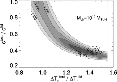
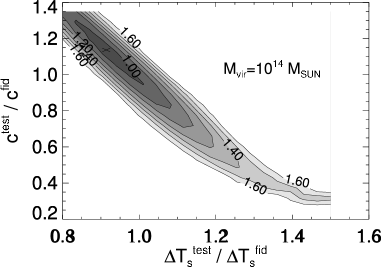
Figure 5.— The $p^{\rm test}=(\Delta T^{\rm test}_{s},c^{\rm test})$ parameter dependence of the $S/N$ ratio for detecting the virial shock of a fiducial cluster with parameters $p^{\rm fid}=(z,\alpha,x_{\mathrm{max}},D)=(0.3,1.5,2c,0.5c)$ and $M_{\mathrm{vir}}=10^{14}{\rm M_{\odot}}$ (lower panel) or $10^{15}{\rm M_{\odot}}$ (upper panel). The fractional change in the S/N is plotted relative to the original S/N in Model II. The contours increase linearly in steps of 0.1 for $\delta S/N>1$, and in steps of 0.05 for $\delta S/N<1$. The test model does not have a virial shock, and its best–fitting parameters are biased. The minima are marked with an X in the upper and lower panels. These values are 0.85 for $(\Delta T^{\rm test}_{0}/\Delta T^{\rm fid},c^{\rm test}_{0}/c^{\rm fid})=(1.38,0.38)$ and 0.94 for $(\Delta T^{\rm test}_{0}/\Delta T^{\rm fid},c^{\rm test}_{0}/c^{\rm fid})=(0.91,1.14)$, respectively. The relatively minor decrease in the S/N indicates that variations in $c$ and $\Delta T_{s}$ cannot mimic the presence of a virial shock, i.e. that the shock remains a distinctive feature.

The numerical results presented in the last section in Table 3 and Figure 3 considered $p^{\rm test}$ parameter values that were equal to the corresponding $p^{\rm fid}$ parameter values. Here we consider the fiducial model with $p^{\rm fid}=(z,\alpha,x_{\mathrm{max}},D)=(0.3,1.5,2c,0.5c)$ and $M_{\mathrm{vir}}=10^{14}{\rm M_{\odot}}$ or $10^{15}{\rm M_{\odot}}$. The fiducial values $(\Delta T^{\rm fid}_{s},c^{\rm fid})$ are calculated from equations (12) and (24) as before. The parameters $p^{\rm test}$ are assumed to be the same for $(M_{\mathrm{vir}},z,\alpha)$ as in the fiducial model, but, in contrast with the previous section, $(\Delta T^{\rm test}_{s},c^{\rm test})$ are allowed to vary relative to the fiducial values.

The fractional deviation of the signal to noise ratio as compared to the original value of test model I for various $p^{\rm test}$ parameters is plotted in Figure 5. The $\sqrt{4/5}$ factor decrease because of the increase in the average noise power is not included in the contour levels for clarity. Thus, the contours have the value of 1.0 at the fiducial parameters. The best fitting parameters $p^{\rm test}_{0}$ correspond to the values at the minimum of S/N.

The most important result from the analysis displayed in Figure 5 is that the signal to noise does not decrease significantly, even in the best–fitting model, relative to the values listed in the previous section (Table 3 and Figure 3). By obtaining the best fit for various $x_{\mathrm{max}}$ we find that the maximum decrease is a factor of $0.95\times\sqrt{4/5},0.9\times\sqrt{4/5}$, and $0.5\times\sqrt{4/5}$ for $M_{\mathrm{vir}}=10^{13}{\rm M_{\odot}},10^{14}{\rm M_{\odot}}$, and $10^{15}{\rm M_{\odot}}$ respectively. The virial shock detection probabilities therefore remain significant for $M_{\mathrm{vir}}=10^{15}{\rm M_{\odot}}$, but become marginal ($S/N\mathrel{\hbox to0.0pt{\lower 4.0pt\hbox{\hskip 1.0pt$\sim$}\hss}\raise 1.0pt\hbox{$<$}}10$) for low–mass clusters ($M_{\mathrm{vir}}\mathrel{\hbox to0.0pt{\lower 4.0pt\hbox{\hskip 1.0pt$\sim$}\hss}\raise 1.0pt\hbox{$<$}}10^{14}{\rm M_{\odot}}$).

Another interesting feature shown in Figure 5 is that the best fitting parameters can deviate significantly from the fiducial values. Changing $M_{\mathrm{vir}}$, $x_{\mathrm{max}}$ and $D$ shows that the $S/N$ of particular clusters can have saddle points and multiple local minima in terms of the $p^{\rm test}$ parameters. We find that this is the case, for example, for $M_{\mathrm{vir}}=10^{14}{\rm M_{\odot}}$ and $1<x_{\mathrm{max}}/c<1.5$, where the local minimum near the fiducial values is not global, and the global minimum $(\Delta T^{\rm test}_{s0},c^{\rm test}_{0})$ instead lies at a much larger SZ temperature and a much smaller concentration. This behavior follows from the fact that decreasing $c$, while fixing all other parameters, produces a steeper $\Delta T^{\rm test}(x)$ profile on log-log scale in the outer regions, a better approximation of the fiducial model with a virial shock. On the other hand, the decrease in $c$ also slightly decreases the SZ temperature in the inner regions, which can be compensated by increasing $\Delta T_{s}$. Overall, a test model profile with a smaller $T_{s}$ and larger $c$ comes closer to the fiducial model.

In Appendix C, we present a simple method to obtain analytical estimates for the best–fitting $p^{\rm test}_{0}$ parameters of a false test model. This approach is fully general, and gives a numerically efficient way to compare two arbitrary models with arbitrary numbers of parameters. Our method is somewhat analogous to a Fisher matrix approach. The standard Fisher matrix treatment serves to estimate the expected uncertainty of the parameters of a correct model. In contrast, the method presented in Appendix C gives an estimate of the best–fitting parameters in an incorrect model (and does not address the uncertainty of these best–fitting values).

7. Parameter estimation

In the previous section, we have examined the signal to noise ratio for distinguishing test models from the fiducial model. The primary aim was to make a distinction between the two basic possibilities, i.e. whether the cluster does or does not have an edge. A more ambitious problem is to examine the precision with which the location and sharpness of the edge can be measured, i.e. the precision of determining the parameters that yield the profile $\Delta T^{\rm fid}(x)$. We calculate the uncertainty of the parameter estimation using both a nonlinear likelihood function directly, and with an approximate Fisher matrix method.

We adopt the fiducial model of the previous section to predict the SZ temperature decrement profile. As before, the fiducial model includes an edge, and is specified by the five parameters $M_{\mathrm{vir}}$, $z$, $\alpha$, $x_{\mathrm{max}}$, and $D$ whose fiducial values will here be collectively denoted by $p^{\rm fid}$. We then compare the temperature decrement in the fiducial model, $\Delta T(x,p^{\rm fid})$, to two different sets of test models. The test models in this case are identical to the fiducial model (i.e., they include an edge), except we allow a subset of the parameters to have values $p^{\rm test}\neq p^{\rm fid}$. These two cases are analogous to the test models I and II in the previous sections. In the first case (Model I), we consider a set of four unknowns $\Delta T_{s}$, $c$, $x_{\mathrm{max}}$, and $D$. In the second case (Model II), we consider only two free variables $x_{\mathrm{max}}$ and $D$, and fix $\Delta T_{s}$ and $c$ at the values calculated in the fiducial model using equations (24) and (12). The other parameters describing the cluster, $M_{\mathrm{vir}}$, $z$, and $\alpha$, are held fixed in both cases.

Now let us suppose that a temperature decrement $\Delta T^{\rm obs}(x)$ is measured, and with no prior information, a parameter $p^{\rm test}$ is to be chosen that best describes the data. Due to random noise, the measurement yields a parameter estimator with some uncertainty. The parameter estimator and its uncertainty can be obtained with the maximum likelihood test, following Appendix A. The likelihood function is

$$L(\Delta T^{\rm obs},p) =P(\Delta T^{\rm obs}\,|\,\Delta T(p))=\frac{1}{(2\pi)^{K/2}(\sigma_{N})^{K}}\times$$ (38)

$$\exp\left(-\frac{K}{2A\,{\sigma_{N}}^{2}}\int\mathrm{d}^{2}x\;[\Delta T^{\rm obs}(x)-\Delta T(x,p)]^{2}\right).$$

The constant normalization pre-factor is irrelevant for the likelihood ratio test, which we hereafter omit from the likelihood function. The log likelihood is

$$\ln L(\Delta T^{\rm obs},p)=-\frac{K}{2A\,{\sigma_{N}}^{2}}\int\mathrm{d}^{2}x\;[\Delta T^{\rm obs}(x)-\Delta T(x,p)]^{2}.$$ (39)

where $K$ and $A$ are the total number of pixels and the surface area of the cluster. The parameters are then chosen to maximize $L(\Delta T^{\rm obs},p)$, or equivalently by applying a least squares fit to the data.

The signal to noise ratio is obtained by the analysis of the projection of the SZ observation profile on the subspace spanned by the fiducial model profiles with arbitrary parameters. The noise power for $N^{\rm fid}$ variable parameters is the variance on this subspace, $N^{2}=N^{\rm fid}\sigma_{N}^{2}$, and the signal to noise ratio is therefore

$$\frac{S^{2}}{N^{2}}=\frac{K}{A\,N^{\rm fid}{\sigma_{N}}^{2}}\int\mathrm{d}^{2}x\;[\Delta T^{\rm fid}(x,p^{\rm test})-\Delta T^{\rm fid}(x,p^{\rm fid})]^{2}$$ (40)

Equation (40) measures the extent that the parameter estimator is $p^{\rm test}$ instead of $p^{\rm fid}$, the true (and maximum likelihood) value. $S^{2}/\sigma_{N}^{2}$ follows $\chi^{2}$-statistics with $N^{\rm fid}$ degrees of freedom, leading to $S^{2}/N^{2}=1\pm\sqrt{2/N^{\rm fid}}$ for $1\sigma$ errors. Given a true parameter set $p^{\rm fid}$, the region within $2\sigma$ confidence (95%) for example is the set of $p^{\rm test}$ values for which $S^{2}/N^{2}<1+2\sqrt{2/N^{\rm fid}}$. The uncertainty of the parameter estimation can therefore be read off directly from equation (40).

Figure 6 shows contour diagrams at fixed values of this uncertainty in Model II, assuming the fiducial parameters $p^{\rm fid}=(z,\alpha,x_{\mathrm{max}},D)=(0.3,1.5,2c,0.5c)$ with $M=10^{14}{\rm M_{\odot}}$ (upper panel) or $M=10^{15}{\rm M_{\odot}}$ (lower panel). The contour plots allow $x_{\mathrm{max}}$ and $D$ to vary, while all other parameters are held fixed at the fiducial values.

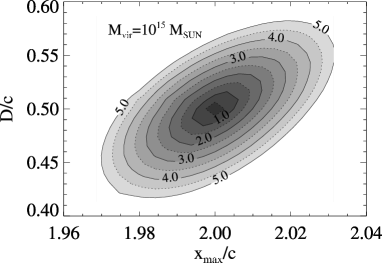
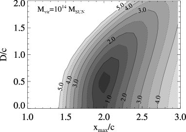
Figure 6.— The $(x^{\rm test}_{\mathrm{max}},D^{\rm test})$ parameter dependence $\chi^{2}$-contours for Model II with $(z,\alpha,x_{\mathrm{max}},D)=(0.3,1.5,2c,0.5c)$, using $M_{\mathrm{vir}}=10^{14}{\rm M_{\odot}}$ (lower panel) and $M_{\mathrm{vir}}=10^{15}{\rm M_{\odot}}$ (upper panel). The contours increase linearly in steps of $0.5\sigma_{N}$.

Figure 6 depicts the likelihood contours for Model II with the direct evaluation of the $S/\sigma_{N}$. An estimate for these contours is provided by the Fisher information matrix,

$$F_{i,j}(p) =-\left\langle\frac{\partial^{2}\ln L(\Delta T^{\rm obs},p)}{\partial p_{i}\partial p_{j}}\right\rangle_{\Delta T^{\rm obs}}$$ (41)

$$=\frac{K}{A\,\sigma_{N}^{2}}\int\mathrm{d}^{2}x\;\frac{\partial\Delta T(x,p^{\rm fid})}{\partial p_{i}}\frac{\partial\Delta T(x,p^{\rm fid})}{\partial p_{j}}.$$ (42)

Assuming that the likelihood distribution is Gaussian near the peak likelihood, we can use confidence limits for Gaussian statistics (i.e., $\chi^{2}$) to obtain $68\%$ and $95\%$ confidence regions. The Fisher matrix greatly speeds up the computations, and allows us to consider additional free parameters (Model I).

The minimum expected variance is related to the Fisher matrix by the Cramer-Rao bound (Tegmark et al., 1997)

$$(\Delta p_{j})^{2}\geq(F^{-1})_{jj}$$ (43)

where equality holds if the distribution is well approximated by a Gaussian distribution.

Tables 5 and 6 show the 68% and 95% significance uncertainties for Models I and II, as calculated from the Fisher matrix. Generally, increasing the number of free variables can increase the uncertainty of the original variables, since a model with additional free parameters can better mimic the fiducial model for a given mock observation. However, our calculations indicate that this is not the case in our case: the uncertainties on $x_{\mathrm{max}}$ and $D$ are nearly the same in Models I and II. This is perhaps unsurprising, since one would not expect that a change in $c$ or $\Delta T_{s}$ (the additional free parameters in Model I) can mimic changes in either $x_{\mathrm{max}}$ and $D$. Indeed, the Fisher matrix is decoupled in the corresponding subspaces, as the $(x_{\mathrm{max}},\Delta T_{s})$, $(x_{\mathrm{max}},c)$, $(D,\Delta T_{s})$, $(D,c)$ components are negligible compared to the diagonal elements. The uncertainties in the parameter estimators are $(\delta c/c,\delta\Delta T_{s}/\Delta T_{s},\delta x_{\mathrm{max}}/x_{\mathrm{max}},\delta D/x_{\mathrm{max}})=(4\%,6\%,9.5\%,25\%)$ for $(M_{\mathrm{vir}},z,\alpha,c,\Delta T_{s},x_{\mathrm{max}},D)=(10^{14}M_{\odot},0.3,1.5,2.9,1.2\mathrm{mK},2c,0.5c)$. Therefore $c$, $\Delta T_{s}$, and $x_{\mathrm{max}}$ will be precisely obtained with ALMA for the majority of the clusters, while similar precision for $D$ is possible for only massive clusters. We note that in principle, it is possible to deduce the value of $\alpha$ directly from the $c(\alpha)$ relation.

Figure 5 provides confidence in our conclusions from the Fisher matrix method: the $1\sigma$ contours in $(x_{\mathrm{max}},D)$ are well-approximated by ellipses, if the fiducial values obey $D-\Delta D>0$, e.g. $D>0.1$, $x_{\mathrm{max}}<1.7c$, and $M_{\mathrm{vir}}\geq 10^{14}{\rm M_{\odot}}$. Therefore, in these cases, the inequality (43) assumes equality for the parameter uncertainty. We find that the parameter distribution around $D\approx 0$ is distorted, and higher confidence level contours for arbitrary $D$ are banana shaped in the $x_{\mathrm{max}}-D$ plane.

Table 5 Parameter uncertainty ($z=0.3$, Model II)

$M_{\mathrm{vir}}$	$\alpha$	$\Theta$	c	$\Delta T_{s}$	$x_{\mathrm{max}}$	$D$	S
$[M_{\odot}]$		[arcmin]		[-muK]	$[c]$	$[c]$	%
$10^{13}$	1	1.8	7.9	23	2	0.5	-
-	-	-	-	-	6.5	17	68
-	-	-	-	-	13	34	95
$10^{13}$	1.5	1.7	4.6	170	2	0.5	-
-	-	-	-	-	6.1	16	68
-	-	-	-	-	12	32	95
$10^{14}$	1	3.8	5.0	140	2	0.5	-
-	-	-	-	-	0.20	0.55	68
-	-	-	-	-	0.41	1.1	95
$10^{14}$	1.5	3.8	2.9	1200	2	0.5	-
-	-	-	-	-	0.19	0.52	68
-	-	-	-	-	0.38	1.04	95
$10^{15}$	1	8.1	3.1	860	2	0.5	-
-	-	-	-	-	0.006	0.018	68
-	-	-	-	-	0.013	0.036	95
$10^{15}$	1.5	8.1	1.8	7900	2	0.5	-
-	-	-	-	-	0.006	0.017	68
-	-	-	-	-	0.012	0.035	95

Table 6 Parameter uncertainty ($z=0.3$, Model I)

$M_{\mathrm{vir}}$	$\alpha$	$\Theta$	c	$\Delta T_{s}$	$x_{\mathrm{max}}$	$D$	S
$[M_{\odot}]$		[arcmin]		[-muK]	$[c]$	$[c]$	%
$10^{13}$	1	1.8	7.9	23	2	0.5	-
-	-	-	1.0	15	6.5	17	68
-	-	-	2.1	29	13	34	95
$10^{13}$	1.5	1.7	4.6	170	2	0.5	-
-	-	-	0.83	132	6.1	16	68
-	-	-	1.7	263	12	32	95
$10^{14}$	1	3.8	5.0	140	2	0.5	-
-	-	-	0.15	6.4	0.21	0.55	68
-	-	-	0.30	13	0.41	1.09	95
$10^{14}$	1.5	3.8	2.9	1200	2	0.5	-
-	-	-	0.11	67	0.19	0.52	68
-	-	-	0.22	135	0.39	1.05	95
$10^{15}$	1	8.1	3.1	860	2	0.5	-
-	-	-	0.013	2.2	0.007	0.018	68
-	-	-	0.026	4.4	0.013	0.036	95
$10^{15}$	1.5	8.1	1.8	7900	2	0.5	-
-	-	-	0.011	27	0.006	0.017	68
-	-	-	0.023	55	0.013	0.035	95

Our calculations show that increasing $x_{\mathrm{max}}$ increases the uncertainties $\Delta x_{\mathrm{max}}$ and $\Delta D$, while increasing $D$ only slightly increases $\Delta x_{\mathrm{max}}$ and leaves $\Delta D$ unchanged. It is clear that the choice of $\alpha$ does not alter the $\Delta x_{\mathrm{max}}$ and $\Delta D$ uncertainties. Changing $z$ yields a maximum in $\Delta x_{\mathrm{max}}$ and $\Delta D$ around $z=0.4$. We find that the parameter uncertainties decrease by a factor of $\sim 10$ at $z\approx 0$ or $z\approx 3$, compared to the $z=0.4$ value.

8. Conclusions

We have shown that the forthcoming Atacama Large Millimeter Array (ALMA) is well–suited for studies of the intra–cluster medium density distribution using the Sunyaev-Zel’dovich (SZ) effect. The angular beam diameter and sensitivities are predicted to reach $2"$ and $10\mu\mathrm{K}$ for this system, which exceed present detector resolutions by more than two orders of magnitude. The SZ decrement profile of a rich galaxy cluster, observed at 100 GHz for $\sim$30 hours, will have a sufficiently high signal-to-noise ratio to make inferences about the gas distributions (and, by inference, about the dark matter distributions).

We solved the equations of hydrostatic equilibrium for the self–similar gas density in the dark matter background. The dark matter profile was parameterized by its inner slope $\alpha$, and every calculation was evaluated for the two values common in the literature, i.e. $\alpha=1$ and 1.5. Within this framework, the density as a function of radial distance is small but nonzero, even in the outer regions. As a modification, we introduced a linear cutoff in the density profile, where the density falls to zero within a finite radial distance. This assumption mimics the presence of strong virial shocks, predicted in cosmological structure formation theories (see Bertschinger 1985 and Bagchi et al. 2002).

We have calculated the SZ decrement profiles of clusters with and without the presence of a sharp density cutoff near the virial radius. We assumed $10\mu\mathrm{K}$ flat-power Gaussian noise. We set up the likelihood function and defined the decision rule to see whether our fiducial model with a virial shock can be distinguished from a test model without a virial shock. It is important to emphasize that this test is practically model–independent: it is only weakly sensitive to the central regions, where cluster models tend to differ, with most of the sensitivity arising from the outer regions, where the various cluster models in the literature are very similar. We calculated the signal to noise ratio in two ways, with either four (Model I) or two (Model II) free parameters. These parameters are the radial distance to the virial shock, $x_{\mathrm{max}}$, the radial thickness of the cutoff, $D$, the concentration parameter, $c$, and the temperature decrement scale, $\Delta T_{s}$, for Model I. For Model II, $c$ and $\Delta T_{s}$ were calculated from theory assuming no scatter around the correct values. Other parameters, such as the virial mass, $M_{\mathrm{vir}}$, the redshift, $z$, and the logarithmic slope of the inner dark matter profile, $\alpha$, can, in principle, be obtained from independent measurements, and were not varied. The signal to noise ratios agree to within 20% in Model I and Model II. The overall value is S/N=470 for a rich cluster of virial mass $10^{15}M_{\odot}$ and we find S/N=16 for a lower–mass cluster with $10^{14}M_{\odot}$.

We also considered a more realistic case, in which the parameters of the cluster with and without a virial shock were fitted independently for a given measurement. We find a large systematic bias in the parameters $c$ and $\Delta T_{s}$ for the model without a virial shock, provided that the cluster does have a virial shock within approximately two virial radius. Nevertheless, the signal to noise ratio decreases only by $50\%$ at most for detecting the virial shock. Therefore, the virial shocks remain detectable for $M\mathrel{\hbox to0.0pt{\lower 4.0pt\hbox{\hskip 1.0pt$\sim$}\hss}\raise 1.0pt\hbox{$>$}}10^{14}{\rm M_{\odot}}$ clusters.

Finally, we examined the precision to which the parameters of the virial shock could be obtained. We find the typical values for the precisions for low–mass ($10^{14}~{}{\rm M_{\odot}}$) and rich ($10^{15}~{}{\rm M_{\odot}}$) clusters to be $(\delta c/c,\delta\Delta T(0)/\Delta T(0),\delta x_{\mathrm{max}}/c,\delta D/x_{\mathrm{max}})=(4\%,6\%,9.5\%,25\%)$ and $(0.6\%,0.3\%,0.3\%,0.9\%)$, respectively. These results assume the cluster is at $z=0.3$, and it is surrounded by a virial shock at twice the virial radius ($x_{\mathrm{max}}=2c$) that has a finite width $D=0.5c$. If the shock was located closer in ($x_{\mathrm{max}}=c$) and was sharper ($D=0.01c$), these uncertainties would improve to $(3.7\%,6.1\%,2.8\%,12\%)$ and $(0.6\%,0.4\%,0.1\%,0.4\%)$, respectively. Since there is a one–to–one theoretical correspondence between $c$ and $\alpha$, with $c(\alpha=1)/c(\alpha=1.5)=1.7$, SZ measurements should help in determining the value of $\alpha$. This should serve as a valuable diagnostic of the inner gas profile; in particular, of the presence of any excess (non–gravitational) entropy that could strongly modify the inner profile.

Our analysis is based on a simplified, spherically symmetric model for the cluster. In these models, the virial shock appears in the SZ surface brightness maps as a full (2$\pi$ azimuthal angle) ring–like feature. In reality, the gas–infall into the cluster potential should be inhomogeneous and anisotropic. As a result, the radial location and the strength of the virial shock will vary in different directions away from the cluster’s center (Evrard, 1990; Bryan & Norman, 1998). We partially accounted for this effect by allowing the virial shock to have a finite width ($D$), which “smears out” the ring–like feature – mimicking the effect of projecting shocks of varying radial locations and strengths. Simulations also show that gas is falling into the cluster potential along overdense filaments, and that the strongest shocks occur along these filaments. If the projected ring–like feature extended over only a fraction $f$ of the full $2\pi$ azimuthal angle (corresponding to the projected areas of the filaments), then our predicted $S/N$ for detecting the virial shock would be further reduced by a factor $1/\sqrt{f}$. The virial shock will nevertheless remain detectable for a $M\sim 10^{15}{\rm M_{\odot}}$ cluster at a significance of $S/N\mathrel{\hbox to0.0pt{\lower 4.0pt\hbox{\hskip 1.0pt$\sim$}\hss}\raise 1.0pt\hbox{$>$}}10$, unless $f\mathrel{\hbox to0.0pt{\lower 4.0pt\hbox{\hskip 1.0pt$\sim$}\hss}\raise 1.0pt\hbox{$<$}}10^{-3}$.

Our results suggest that SZ decrement measurements with ALMA can reveal virial shocks around galaxy clusters, and can determine the location and size of these shocks with high precision. This will provide a unique constraint on theories of large–scale structure formation.

APPENDIX A: DISTINGUISHING MODELS WITH THE OPTIMAL FILTER

In this appendix, we give a formal summary of the treatment of the following general problem. Consider a system that obeys laws that predict a set of observables ${\bf h}^{\rm fid}$. What is the significance at which a false hypothesis, predicting a different set of observables, ${\bf h}^{\rm test}$, can be rejected, given the presence of Gaussian random noise?

A measurement of the observable in $x_{K}$ distinct directions yields a discrete sample $y_{k}$ where $k\in[1,K]$. The set $\{y_{k}\}$ is an element of a $K$-dimensional vector space and will be denoted by ${\bf y}$. Similarly, let ${\bf h}^{\rm fid}$ and ${\bf h}^{\rm test}$ denote the discrete sample of the hypotheses functions $h^{\rm fid}(x)$ and $h^{\rm test}(x)$. In our example, ${\bf y}$ denotes a measured SZE temperature profile, whereas ${\bf h}^{\rm fid}$ and ${\bf h}^{\rm test}$ denote the discrete temperature profiles predicted in models with and without a cutoff. The vectors ${\bf h}^{\rm fid}$ and ${\bf h}^{\rm test}$ depend on the parameters describing the cluster and the cutoff. We now derive the signficance (or “signal to noise ratio”) of distinguishing between two models.

If the real signal arriving to the detector was $s(x)$, then the detector measures the data

$${\bf y}={\bf s}+{\bf n}$$ (44)

where ${\bf n}$ is a random variable, corresponding to the noise. Let us assume white Gaussian noise of variance $\sigma_{N}^{2}$. In this case, the probability of detecting ${\bf y}$, given that the incoming signal is ${\bf s}$, is

$$P({\bf y}\,|\,{\bf s})=\frac{1}{(2\pi)^{K/2}(\sigma_{N})^{K}}\exp\left[-\frac{({\bf y}-{\bf s})^{2}}{2\sigma_{N}^{2}}\right],$$ (45)

where the arithmetic (difference and scalar product) of the K-dimensional vectors was used, i.e.

$$({\bf y}-{\bf s})^{2}=\sum_{k=1}^{K}(y_{k}-s_{k})^{2}.$$ (46)

Two hypotheses can be distinguished using $P({\bf s}\,|\,{\bf y})$, which can be obtained from $P({\bf y}\,|\,{\bf s})$ and the a–priori probabilities $P({\bf s})$ by applying the Bayes theorem for conditional probabilities. Most common decision rules, such as the maximum posteriori, the Neyman-Pearson, or the minimax decisions (e.g. Whalen 1971) involve constraints on the likelihood ratio,

$$L({\bf y})=\frac{P({\bf y}\,|\,{\bf h}^{\rm test})}{P({\bf y}\,|\,{\bf h}^{\rm fid})}.$$ (47)

Substituting (45) in (47) the log–likelihood becomes

$$\ln L({\bf y})=\frac{1}{\sigma_{N}^{2}}({\bf h}^{\rm test}-{\bf h}^{\rm fid})\cdot({\bf y}-{\bf h}^{\rm fid})-\frac{1}{2\sigma_{N}^{2}}({\bf h}^{\rm test}-{\bf h}^{\rm fid})^{2}$$ (48)

The decision is made in favor of the test hypothesis if the likelihood ratio exceeds a given threshold. The likelihood depends on the ${\bf y}-{\bf h}^{\rm fid}$ component along ${\bf h}^{\rm test}-{\bf h}^{\rm fid}$. The term ${\bf h}^{\rm test}-{\bf h}^{\rm fid}$ is referred to as the matched filter, which is the optimal filter for the distinction of the two hypotheses in white Gaussian noise.

Since the noise distribution $P({\bf n})$ is spherically symmetric in the K-dimensional vector space, it has the same power $\sigma_{N}^{2}$ along any basis. This implies that the noise power for the likelihood detection rule is the noise power for a single bin, i.e. $N^{2}=\sigma_{N}^{2}$. Thus increasing the sample size increases the signal power, but leaves the relevant noise contribution the same.

The signal power is

$$S^{2}=({\bf h}^{\rm test}-{\bf h}^{\rm fid})^{2}=\sum_{k}(h^{\rm test}_{k}-h^{\rm fid}_{k})^{2}=\frac{1}{\Delta x^{2}}\int\mathrm{d}^{2}x\;\Delta h(x)^{2},$$ (49)

where $\Delta h(x)=h^{\rm test}(x)-h^{\rm fid}(x)$ and $\Delta x^{2}$ denotes the area enclosed by the neighboring $x_{k}$ points. We have assumed that the resolution of the measurement is fine enough to approximate the sum with the integral. Therefore, the signal to noise ratio is

$$\frac{S^{2}}{N^{2}}=\frac{({\bf h}^{\rm test}-{\bf h}^{\rm fid})^{2}}{\sigma_{N}^{2}}.$$ (50)

The signal to noise ratio is an important measure of the significance of the test. Let us define $\rho$ as a one-dimensional random variable by

$$\rho(\bf y)=\frac{({\bf h}^{\rm test}-{\bf h}^{\rm fid})\cdot({\bf y}-{\bf h}^{\rm fid})}{||{\bf h}^{\rm test}-{\bf h}^{\rm fid}||\,\sigma_{N}}$$ (51)

for which $P(\rho\,|\,{\bf s}={\bf h}^{\rm fid})$ is a standard normal distribution, whereas $P(\rho\,|\,{\bf s}={\bf h}^{\rm test})$ is a normal distribution with mean $S/N$ and unit variance. Thus, if the fiducial model is true, $\rho^{2}$ follows $\chi^{2}$ statistics, and the significance of the test can be obtained by comparing $S^{2}/N^{2}$ with the $\chi^{2}$ confidence levels.

In our case, for a detector with angular resolution $\Delta\phi$ and a cluster of apparent angular virial radius $\Theta$ the surface element is $\Delta x^{2}=A/K$, where $K=(x^{\rm test}_{\mathrm{max}}\Theta)^{2}/(c\Delta\phi)^{2}$ is the total number of pixels and $A=\pi{x^{\rm test}_{\mathrm{max}}}^{2}$ is the surface area of the cluster. Therefore,

$$\frac{S}{N}=\frac{\Theta}{\sqrt{\pi}\,c\,\Delta\phi\,\sigma_{N}}\sqrt{\int\mathrm{d}^{2}x\,[h^{\rm test}(x)-h^{\rm fid}(x)]^{2}}.$$ (52)

is the signal to noise ratio for the decision between the two hypotheses.

APPENDIX B: DISTINGUISHING MODELS WITH FREE PARAMETERS

Here we address the following problem, which is a generalized version of the problem posed in Appendix A above. Consider again a system that obeys laws that predict a set of observables ${\bf h}^{\rm fid}$. What is the significance at which a false hypothesis, predicting a different set of observables, ${\bf h}^{\rm test}$, can be rejected, given the presence of a Gaussian random noise, if the parameters of the false test model are not known a priori and can be freely adjusted?

Assume that the original signal (i.e. without noise) is ${\bf h}^{\rm fid}$ with a set of $N^{\rm fid}$ parameters, $p^{\rm fid}_{0}$, and the false hypotheses is described by $N^{\rm test}$ parameters, $p^{\rm test}$. The measurement

$${\bf y}={\bf h}^{\rm fid}(p^{\rm fid}_{0})+{\bf n}$$ (53)

can be used to give an estimate of $p^{\rm fid}_{0}$. As in Appendix A, ${\bf y}$ is the collection of $K$ observables (e.g. the SZ brightness of the $K$ pixels), and ${\bf n}$ is a $K$-dimensional Gaussian random variable. Denote the estimated parameter of ${\bf h}^{\rm fid}$ by $p^{\rm fid}$ and the estimated parameter of ${\bf h}^{\rm test}$ by $p^{\rm test}$. Once the parameters have been obtained, ${\bf h}^{\rm fid}(p^{\rm fid})$ and ${\bf h}^{\rm test}(p^{\rm test})$ can be fixed at the corresponding values. Then the likelihood ratio for fixed parameters can be used, according to equation (48), and the decision is made in favor of the test model rather than the fiducial model exactly if the likelihood is above a given threshold.

Since $p^{\rm fid}$ is obtained by minimizing $({\bf y}-{\bf h}^{\rm fid}(p^{\rm fid}))^{2}$, the distribution of ${\bf h}^{\rm fid}(p^{\rm fid})$ from (53) is

$${\bf h}^{\rm fid}(p^{\rm fid})={\bf h}^{\rm fid}(p^{\rm fid}_{0})+\bm{\Delta}_{1},$$ (54)

where $p^{\rm fid}_{0}$ is the real parameter of the signal without the noise and $\bm{\Delta}_{1}$ is an $N^{\rm fid}$ dimensional Gaussian random variable. $\bm{\Delta}_{1}$ has zero mean and variance $N^{\rm fid}\sigma_{N}^{2}$. Similarly, $p^{\rm test}$ is obtained by minimizing $({\bf y}-{\bf h}^{\rm test}(p^{\rm test}))^{2}$. The distribution of ${\bf h}^{\rm test}(p^{\rm test})$ is

$${\bf h}^{\rm test}(p^{\rm test})={\bf h}^{\rm test}(p^{\rm test}_{0})+\bm{\Delta}_{2}$$ (55)

where $p^{\rm test}_{0}$ is the $p^{\rm test}$ parameter value at which $({\bf h}^{\rm fid}(p^{\rm fid}_{0})-{\bf h}^{\rm test}(p^{\rm test}))^{2}$ is minimal. $\bm{\Delta}_{2}$ is defined by equation (55), which is an $N^{\rm test}$-dimensional Gaussian random variable, with zero mean and variance $N^{\rm test}\sigma_{N}^{2}$. Note that $\bm{\Delta}_{1}$ and $\bm{\Delta}_{2}$ are strongly correlated since both values are derived from the same measurement ${\bf y}$.

The signal power

$$S^{2}=({\bf h}^{\rm test}-{\bf h}^{\rm fid})^{2}$$ (56)

is therefore a random variable. Let us define the empirical, most probable and expected signal powers by

$$S_{\rm emp}^{2} =({\bf h}^{\rm test}(p^{\rm test})-{\bf h}^{\rm fid}(p^{\rm fid}))^{2}$$ (57)

$$S_{0}^{2} =({\bf h}^{\rm test}(p^{\rm test}_{0})-{\bf h}^{\rm fid}(p^{\rm fid}_{0}))^{2}=\min_{p^{\rm test}}({\bf h}^{\rm test}(p^{\rm test})-{\bf h}^{\rm fid}(p^{\rm fid}_{0}))^{2}$$ (58)

$$S_{\rm exp}^{2} =\langle S_{\rm emp}^{2}\rangle_{p^{\rm test},p^{\rm fid}}.$$ (59)

The expected signal power can be written in terms of $S_{0}$ using eqs. (54) and (55)

$$S_{\rm exp}^{2} =\langle[{\bf h}^{\rm test}(p^{\rm test}_{0})-{\bf h}^{\rm fid}(p^{\rm fid}_{0})+\bm{\Delta}_{2}-\bm{\Delta}_{1}]^{2}\rangle$$ (60)

$$=S_{0}^{2}+\langle(\bm{\Delta}_{2}-\bm{\Delta}_{1})^{2}\rangle$$ (61)

$$=S_{0}^{2}+\langle\bm{\Delta}_{2}^{2}\rangle+\langle\bm{\Delta}_{1}^{2}\rangle-2\langle\bm{\Delta}_{1}\bm{\Delta}_{2}\rangle$$ (62)

$$=S_{0}^{2}+(N^{\rm fid}+N^{\rm test})\sigma_{N}^{2}-2\langle\bm{\Delta}_{1}\bm{\Delta}_{2}\rangle.$$ (63)

In particular if $N^{\rm fid}=N^{\rm test}=1$, then $\langle\bm{\Delta}_{1}\bm{\Delta}_{2}\rangle=\cos(\phi)\sigma_{N}^{2}/2$. This term can be obtained, for given ${\bf h}^{\rm fid}$ and ${\bf h}^{\rm test}$ hypothesis functions by

$$\cos(\phi)=\frac{\left|\frac{\mathrm{d}{\bf h}^{\rm fid}(p^{\rm fid}_{0})}{\mathrm{d}p^{\rm fid}_{0}}\cdot\frac{\mathrm{d}{\bf h}^{\rm test}(p^{\rm test}_{0})}{\mathrm{d}p^{\rm test}_{0}}\right|}{\left|\frac{\mathrm{d}{\bf h}^{\rm fid}(p^{\rm fid}_{0})}{\mathrm{d}p^{\rm fid}_{0}}\right|\left|\frac{\mathrm{d}{\bf h}^{\rm test}(p^{\rm test}_{0})}{\mathrm{d}p^{\rm test}_{0}}\right|}.$$ (64)

For arbitrary numbers of parameters, the expected value of $\langle\bm{\Delta}_{1}\bm{\Delta}_{2}\rangle$ has a more complicated algebraic form, but can always be obtained for a specific choice of ${\bf h}^{\rm fid}$ and ${\bf h}^{\rm test}$ functions. For simplicity we shall restrict only to the inequality

$$\langle\bm{\Delta}_{1}\bm{\Delta}_{2}\rangle\geq 0,$$ (65)

leading to

$$S_{0}^{2}\leq S_{\rm exp}^{2}\leq S_{0}^{2}+(N^{\rm fid}+N^{\rm test})\sigma_{N}^{2}.$$ (66)

The noise power for choosing between ${\bf h}^{\rm fid}$ and ${\bf h}^{\rm test}$ (with an arbitrary $p^{\rm fid}$ or $p^{\rm test}$) is the variance of the measurement along ${\bf h}^{\rm test}(p^{\rm test})-{\bf h}^{\rm fid}(p^{\rm fid})$, since the likelihood ratio (48) depends on only this component. Therefore

$$N_{\rm exp}^{2} =\left<\left[\frac{{\mathbf{h}}^{\rm test}(p^{\rm test})-{\bf h}^{\rm fid}(p^{\rm fid})}{||{\bf h}^{\rm test}(p^{\rm test})-{\bf h}^{\rm fid}(p^{\rm fid})||}\cdot({\bf y}-{\bf h}^{\rm fid}(p^{\rm fid}))\right]^{2}\right>$$ (67)

$$=\sigma_{N}^{2}+\left<\left[\frac{{\bf h}^{\rm test}(p^{\rm test})-{\bf h}^{\rm fid}(p^{\rm fid})}{||{\bf h}^{\rm test}(p^{\rm test})-{\bf h}^{\rm fid}(p^{\rm fid})||}\cdot\bm{\Delta}_{1}\right]^{2}\right>.$$ (68)

For large signal to noise ratios this can be approximated to lowest order in $\bm{\Delta}_{1}$.

$$N_{\rm exp}^{2} =\sigma_{N}^{2}+\left<\left[\frac{{\bf h}^{\rm test}(p^{\rm test}_{0})-{\bf h}^{\rm fid}(p^{\rm fid}_{0})}{||{\bf h}^{\rm test}(p^{\rm test}_{0})-{\bf h}^{\rm fid}(p^{\rm fid}_{0})||}\cdot\bm{\Delta}_{1}\right]^{2}\right>$$ (69)

$$=\sigma_{N}^{2}+\langle(\cos\theta)^{2}\rangle\sigma_{N}^{2},$$ (70)

where $\theta$ is the angle between the vector ${\bf h}^{\rm test}(p^{\rm test}_{0})-{\bf h}^{\rm fid}(p^{\rm fid}_{0})$ and ${\bf h}^{\rm fid}(p^{\rm fid})-{\bf h}^{\rm fid}(p^{\rm fid}_{0})$. In general for any $({\bf h}^{\rm fid},{\bf h}^{\rm test})$

$$\sigma_{N}^{2}\leq N_{\rm exp}^{2}\leq 2\sigma_{N}^{2}.$$ (71)

Equation (71) is a natural consequence of the fact that there are two sources of uncertainties for the hypothesis test, corresponding to the uncertain estimates of the parameters of the fiducial and test models. In principle, these uncertainties can add up constructively to create a $2\sigma_{N}^{2}$ variance in the likelihood ratio, but the noise power is at least the noise of the fixed models of Appendix A, $1\sigma_{N}^{2}$.

In particular, for the SZE brightness hypotheses, the test model is a special case of the fiducial model, with the fiducial model having two additional parameters describing the cutoff at the virial shock. In this case for $N^{\rm fid}=4$ and $N^{\rm test}=2$, it can be shown that $\langle(\cos\theta)^{2}\rangle\approx 1/4$ independent of $p^{\rm fid}_{0}$. Therefore

$$N_{\rm exp}^{2}=\frac{5}{4}\sigma_{N}^{2}.$$ (72)

Although the expected signal to noise ratio can be calculated explicitly for a given parameter choice using equation (63) and (72), it is useful to define its the theoretical bounds independent of the given form of the hypotheses. Comparing equations (66) and (71), we obtain

$$\frac{S_{0}^{2}}{2\sigma_{N}^{2}}\leq\frac{S_{\rm exp}^{2}}{N_{\rm exp}^{2}}\leq\frac{S_{0}^{2}}{\sigma_{N}^{2}}+N^{\rm fid}+N^{\rm test},$$ (73)

where $S_{0}$ is given by equation (58). The high bound is approached when $H^{\rm test}$ tends to be parallel to $H^{\rm fid}$, the low bound is approached when $H^{\rm test}$ is orthogonal to $H^{\rm fid}$ near $H^{\rm fid}(p^{\rm fid}_{0})$ and $H^{\rm test}(p^{\rm test}_{0})$. Here $H$ denotes the sub–space of the K–dimensional vector space that is spanned by the variable parameters.

APPENDIX C: PARAMETER BIAS FOR A FALSE HYPOTHESIS

Here we present an estimate for the values of the best–fitting parameters of a false hypothesis. This problem can be contrasted with the application of the Fisher matrix. While the latter is a method to obtain the variance on the parameters of the true model, here we seek an approximation of the expectation values for the best-fitting parameters of a false test model (regardless of the uncertainties around this best fit, and whether the best is an acceptable fit).

Finding $p^{\rm test}_{0}$, the minimum value in the $p^{\rm test}$ parameter space in general can be computationally tedious. Our treatment is general as long as the fiducial hypotheses has all of the parameters of the test hypotheses plus some additional parameters and if the two hypotheses deviate by only a reasonably small amount. In particular, as displayed in the panels of Figure 5, the numerical value obtained naively by

$${p^{\rm test}_{0}}^{(0)}=(\Delta T^{\rm test}_{s},c^{\rm test})=(\Delta T^{\rm fid}_{s},c^{\rm fid})$$ (74)

is a fair zeroth approximation for the two cluster models in most cases. A better approximation can be obtained by expanding $[{\bf h}^{\rm test}(p^{\rm test})-{\bf h}^{\rm fid}(p^{\rm fid})]^{2}$ to second order around ${p^{\rm test}_{0}}^{(0)}$ and finding its minimum in terms of $p^{\rm test}$.

$$({\bf h}^{\rm test}(p^{\rm test}_{0}) -{\bf h}^{\rm fid}(p^{\rm fid}))^{2}\approx$$

$$({\bf h}^{\rm test}-{\bf h}^{\rm fid})^{2}+2(\partial_{k}{\bf h}^{\rm test})\cdot({\bf h}^{\rm test}-{\bf h}^{\rm fid})x_{k}$$ (75)

$$+[(\partial_{j}{\bf h}^{\rm test})\cdot(\partial_{k}{\bf h}^{\rm test})+\partial_{j}\partial_{k}{\bf h}^{\rm test}\cdot({\bf h}^{\rm test}-{\bf h}^{\rm fid})]x_{j}x_{k}$$

where it is assumed that ${\bf h}^{\rm test}$ and ${\bf h}^{\rm fid}$ are evaluated at ${p^{\rm test}_{0}}^{(0)}$ and $p^{\rm fid}$, respectively. The indices $j$ and $k$ run across the test model parameters, and $x_{k}={p^{\rm test}_{0}}^{(1)}_{k}-{p^{\rm test}_{0}}^{(0)}_{k}$, furthermore

$$\partial_{k}=\frac{\partial}{\partial{p^{\rm test}}_{k}}.$$ (76)

Let us denote the quadratic coefficient by

$$M_{kj}=(\partial_{k}{\bf h}^{\rm test})\cdot(\partial_{j}{\bf h}^{\rm test})+({\bf h}^{\rm test}-{\bf h}^{\rm fid})\cdot\partial_{k}\partial_{j}{\bf h}^{\rm test}.$$ (77)

Equation (75) gives the deviation of the signal to noise ratio if the test model parameters are modified from the fiducial values. The expected signal to noise corresponds to the minimum value in terms of $x_{k}$, at which the $x_{k}$ derivative must vanish

$$\frac{\partial}{\partial x_{k}}[h^{\rm test}(p^{\rm test}_{0}) -{\bf h}^{\rm fid}(p^{\rm fid})]^{2}\approx$$ (78)

$$2(\partial_{k}{\bf h}^{\rm test})\cdot({\bf h}^{\rm test}-{\bf h}^{\rm fid})+2M_{kj}x_{j}=0.$$

Since $x_{k}={p^{\rm test}_{0}}^{(1)}_{k}-{p^{\rm test}_{0}}^{(0)}_{k}$, the solution of this equation gives the next approximation of $p^{\rm test}_{0}$. Equation (78) is solved by inverting the coefficient matrix. Thus

$${p^{\rm test}_{0}}^{(1)}_{k}={p^{\rm test}_{0}}^{(0)}_{k}-M_{kj}^{-1}(\partial_{j}{\bf h}^{\rm test})\cdot({\bf h}^{\rm test}-{\bf h}^{\rm fid}),$$ (79)

${p^{\rm test}_{0}}^{(1)}_{k}$ is the improved approximation of the $k^{\mathrm{th}}$ parameter of ${p^{\rm test}_{0}}$. Note that the $\Delta T_{s}$-dependence of the hypotheses is linear, implying $\partial_{\Delta T_{s}}{\bf h}^{\rm test}(p^{\rm test})={\bf h}^{\rm test}(c^{\rm test},\Delta T^{\rm test}_{s}=1)$ and $\partial^{2}_{\Delta T_{s}}{\bf h}^{\rm test}(p^{\rm test})=0$ for all $p^{\rm test}$. The $c^{\rm test}$ parameter derivatives are to be calculated numerically using equation (23). In conclusion, finding the minimum in equation (37) is simplified to evaluating parameter derivatives of the ${\bf h}^{\rm test}$ function at only ${p^{\rm test}_{0}}^{(0)}$.

Figure 5 shows how the best fitting ${p^{\rm test}_{0}}$ parameters are related to the naive choice $p^{\rm fid}$ when detecting virialization shocks with the SZ effect. The $S/N$ function has a minimum at ${p^{\rm test}_{0}}$. Finding the critical point with equation (79) yields the correct global minimum for $(M_{\mathrm{vir}},z,\alpha)=(10^{13}M_{\odot},0.3,1.5)$ for any $(x_{\mathrm{max}},D)$ and $(10^{14}M_{\odot},0.3,1.5)$ for any $(x_{\mathrm{max}},D)$ unless $x_{\mathrm{max}}\approx c$. However, for $(M_{\mathrm{vir}},z,\alpha,x_{\mathrm{max}})\approx(10^{14}M_{\odot},0.3,1.5,c)$ there are multiple local minima and saddle points. The ${p^{\rm test}_{0}}={p^{\rm test}_{0}}^{(1)}$ approximation of equation (79) yields the local minima in the vicinity, which is not the global minimum. For $(M_{\mathrm{vir}},z,\alpha)\approx(10^{15}M_{\odot},0.3,1.5)$ and arbitrary $(x_{\mathrm{max}},D)$, the ${p^{\rm test}_{0}}^{(1)}$ value corresponds to the saddle point. Again, the ${p^{\rm test}_{0}}={p^{\rm test}_{0}}^{(1)}$ approximation of equation (79) breaks down.

The saddle points can be identified by calculating $\det M_{i,j}$

$$\det M_{kj}(p^{test})\begin{array}[]{ll}>0&\text{iff $p^{test}$ is at a local minimum or maximum}\\ <0&\text{iff $p^{test}$ is at a saddle point}\\ \end{array}$$ (80)

The saddle point can be eluded if $\det M_{kj}$ is calculated and a step is made towards ${p^{\rm test}_{0}}^{(1)}$ only if $\det M_{kj}>0$. If it is negative, then a step is made ”downhill” along the negative gradient $-2(\partial_{k}{\bf h}^{\rm test})\cdot({\bf h}^{\rm test}-{\bf h}^{\rm fid})$.

Repeating equation (79) or the downhill steps gives a numerical efficient way of obtaining better and better approximations of the best fit test parameter values near the corresponding fiducial parameters. Further study shows that this algorithm leads to the correct ${p^{\rm test}_{0}}$ value in most cases. Only the fiducial parameters around $p=(M_{\mathrm{vir}},z,\alpha)\approx(10^{14}M_{\odot},0.3,1.5)$, with $(x_{\mathrm{max}},D)=(c,0.01c)$ or $(c,0.5c)$ have non-global minimum in the close neighborhood of $p^{\rm fid}_{0}$. In this case the best fitting test model parameters have to be obtained by evaluating equation (58) at multiple parameter values, scanning the parameter space.

References

- Bagchi et al. (2002) Bagchi, J. 2002, NewA, 7, 249B
- Barbosa et al. (1996) Barbosa, D., Bartlett, J., Blanchard, A., & Oukbir, J. 1996, A&A, 314, 13
- Bartlett (2001) Bartlett, J.G. 2001, A&A, preprint astro-ph/0001267
- Bertschinger (1985) Bertschinger E. 1985, ApJS, 58, 39
- Birnboim & Dekel (2003) Birnboim, Y., & Dekel, A. 2003, MNRAS, 345, 349
- Birkinshaw (1999) Birkinshaw, M. 1999, Physics Reports, 310, 97
- Bryan & Norman (1998) Bryan, G. L. & Norman, M. L. 1998, ApJ, 495, 80
- Butler et al. (1999) Butler, B. et al. 1999, MMA Memo. No. 243
- Carlstrom et al. (2002) Carlstrom, J., Holder, G., & Reese, E. D. 2002, ARA&A, 40, 643
- Eke et al. (2001) Eke V. R., Navarro J. F., & Steinmetz M., 2001, ApJ, 469, 494
- Evrard (1997) Evrard, A. E. 1997, MNRAS, 292, 289
- Evrard (1990) Evrard, A. E. 1990, ApJ, 363, 349
- Haiman et al. (2001) Haiman, Z., Mohr, J. J., & Holder, G. P. 2001, ApJ, 553, 545
- Holdaway & Juan (1999) Holdaway, M. A., & Juan, R. P. 1999, MMA Memo. No. 187
- Holder et al. (2000) Holder, G., Mohr, J., Carlstrom, J., Evrard, A., & Leitch, E. M. 2000, ApJ, 544, 629
- Holder & Carlstrom (2001) Holder, G., & Carlstrom, J. E. 2001, ApJ, 558, 515
- Holder (2004) Holder, G., 2004, ApJ, 602, 18
- Hu & Dodelson (2002) Hu, W., & Dodelson, S. 2002, ARA&A, 40, 171
- Jing & Suto (2000) Jing Y. P., & Suto Y. 2000, ApJ, 529, L69
- Keres et al. (2004) Keres, D., Katz, N., Weinberg, D. H., & Davé, R. 2004, MNRAS, submitted, astro-ph/0407095
- Kneissl et al. (2001) Kneissl, R., Jones, M. E., Saunders, R., Eke, V. R., Lasenby, A. N., Grainge, K., & Cotter, G. 2001, MNRAS, 328, 783
- Komatsu & Seljak (2001) Komatsu, E., & Seljak, U. 2001, MNRAS, 327, 1353
- Komatsu & Seljak (2002) Komatsu, E., & Seljak, U. 2002, MNRAS, 336, 1256
- Loeb & Waxman (2000) Loeb, A., & Waxman, E. 2000, Nature, 405, 156
- Moore et al. (1999) Moore, B. et al. 1999, MNRAS, 310, 1147
- Navarro et al. (1997) Navarro J. F., Frenk C. S., & White S. D. M. 1997, ApJ, 490, 493
- Peebles (1993) Peebles, P. J. E. 1993, Principles of Physical Cosmology, Princeton University Press, Princeton
- Pen (1999) Pen, U. 1999, preprint astro-ph/9904172
- Rees & Ostriker (1977) Rees, M. J., & Ostriker, J. P. 1977, ApJ, 179, 541
- Rines et al. (2003) Rines, K., Geller, M. J., Kurtz, M. J., Diaferio, AJ, 126, 2152
- Spergel et al. (2003) Spergel, D. N. et al. 2003, AJS, 148, 175
- Springel et al. (2001) Springel, V., White, M., & Hernquist, L. 2001, ApJ, 549, 681
- Sunyaev & Zeldovich (1980) Sunyaev, R. A., & Zel’dovich, Ya. B. 1980, ARA&A, 18, 537
- Suto et al. (1998) Suto Y., Sasaki S., & Makino N. 1998, ApJ, 509, 544
- Tegmark et al. (1997) Tegmark, M., Taylor, A. N., & Heavens, A. F. 1997, ApJ, 480, 22
- Tozzi et al. (2000) Tozzi, P., Scharf, C., & Norman, C. 2000, ApJ, 542, 106
- Verde et al. (2002) Verde, L., Haiman, Z., & Spergel, D. N. 2002, ApJ, 581, 5
- Whalen (1971) A. D. Whalen, Detection of Signals in Noise, Academic Press, New York, 1971