Investigations of Lepton and Baryon Acceleration in Relativistic Astrophysical Shocks

Abstract

Double, Glen Paul. Investigations of Lepton and Baryon Acceleration in Relativistic Astrophysical Shocks. (Under the direction of Donald C. Ellison.)

Gamma-ray bursts, occurring randomly each day anywhere in the universe, may be the brightest objects in the sky during their short life. Particle acceleration in mildly relativistic shocks, internal to the main blastwave, may explain the early intensity peaks in gamma-ray bursts and the afterglow may be explained by energetic particles accelerated by the main ultrarelativistic blastwave shock as it slows to the mildly relativistic range. To help explain the phenomena, a nonlinear relativistic Monte Carlo model was developed and used to study lepton and baryon acceleration by mildly relativistic modified shocks with the magnetic field parallel to the shock normal. The study showed that for equal densities of leptons and baryons, lepton acceleration is highly sensitive to the shock velocity profile. With the shock fully modified by energetic baryons, the injection efficiency of leptons, relative to baryons, increases with Lorentz factor, and injection efficiency will reach a maximum well below that of baryons at the same momentum. Given the assumptions in this model, if the particles are energized by shock acceleration, leptons will always carry far less energy than baryons when the lepton and baryon densities are of the same order. It was determined that the lepton to baryon number density ratio must be approximately $3\times 10^{5}$ for both species to equally share the kinetic energy of the shock. This energy equipartition density ratio is independent of shock speed over the range of mildly relativistic Lorentz factors used in the study, but the result may extend to ultrarelativistic speeds. The study was a special case of a larger effort that will include relativistic oblique modified shocks and computer generated gamma-ray spectra when the model is completed. New magnetohydrodynamic conservation laws and relativistic jump conditions were developed for the model, along with a new equation of state and a new method for estimating the adiabatic index in the mildly relativistic range. The present state of the model shows smooth transitions of shock parameters from nonrelativistic to highly relativistic unmodified shocks while allowing oblique magnetic fields and a pressure tensor.

INVESTIGATIONS OF LEPTON AND BARYON ACCELERATION IN RELATIVISTIC ASTROPHYSICAL SHOCKS

by
Glen Paul Double

a dissertation submitted to the graduate faculty of
north carolina state university
in partial fulfillment of the
requirements for the degree of
doctor of philosphy
 
department of physics

raleigh
March 2024

approved by:
 
 
Dr. Mohamed A. Bourham Dr. Dean J. Lee Minor Representative Member of Advisory Committee Dr. John M. Blondin Dr. Donald C. Ellison Member of Advisory Committee Chairman of Advisory Committee

Table of Contents

toc

List of Figures

lof

List of Symbols

SYMBOL		DEFINITION
$\alpha$	-	anisotropy parameter for tensor pressure
$\beta$	-	dimensionless speed, normalized by c
$c$	-	speed of light (299792458 meters/second)
$\gamma$	-	Lorentz factor $(1-\beta^{2})^{-\frac{1}{2}}$
$\gamma_{0}$	-	Lorentz factor of shock speed or far upstream flow speed; also called $\gamma_{\mathrm{sk}}$
$\Gamma$	-	adiabatic index
GRB	-	Gamma-ray burst
$\epsilon_{0}$	-	permittivity of free space
$\epsilon_{\mathrm{inj}}$	-	injection efficiency
$\eta$	-	gyrofactor that scales the gyroradius $r_{g}$
$e$	-	total energy density
$eV$	-	electron volt
$f_{s}$	-	normalized subshock size
ISM	-	Interstellar medium; the space between the stars
$k$	-	Boltmann’s constant
$\kappa$	-	Diffusion coefficient
$\lambda$	-	Mean free path
$\lambda_{D}$	-	Debye length
$L$	-	Diffusion Length
$\mu_{0}$	-	permeability of free space
$n$	-	particle number density
$p$	-	particle momentum
$P_{\parallel}$	-	fluid pressure along the magnetic field vector
$P_{\perp}$	-	fluid pressure perpendicular to the magnetic field vector
$P_{R}$	-	Probability of return function
$q$	-	unit electric charge
$\rho_{q}$	-	electric charge density
$\rho$	-	rest mass density
$r$	-	shock compression ratio ($u_{0}/u_{2}$)
$r_{g}$	-	gyroradius for a charged particle orbiting in a magnetic field
$r_{s}$	-	subshock compression ratio ($u_{1}/u_{2}$)
$\sigma$	-	spectral index; the magnitude of a power law slope
$\Theta_{Bn}$	-	angle between the magnetic field and the shock normal
$\mathcal{T}$	-	temperature associated with kinetic energy of the particle ensemble
$u_{0}$	-	shock speed or far upstream flow speed seen from the shock frame
$u_{1}$	-	flow speed at the shock (subshock), as measured in the shock frame
$u_{2}$	-	flow speed far downstream seen in the shock frame
$v$	-	particle speed
$w$	-	enthalpy ($e+P$) density or specific enthalpy
$Z$	-	total electric charge number of an ion

Chapter 1 Introduction

Shock waves occur in fluids whenever a disturbance propagates faster than the characteristic speed of sound in the fluid. The same phenomena occur in space where the fluid is a plasma consisting of positively and negatively charged particles permeated by magnetic fields and negligible electric fields.

In space where the particle density is low, typically a few particles per cubic centimeter, shock waves are collisionless rather than acoustic-ion shocks because the effective diffusion length due to charged particles interacting with the magnetic field is generally much shorter than the mean free path between particles. An acoustic-ion shock wave propagates by Coulomb forces, for example shock waves in the Earth’s atmosphere, but collisionless shocks propagate through disturbances in the magnetic field of the space plasma.

Shock waves are found throughout the universe. Examples of nonrelativistic shocks range from transient disturbances on the surface of the sun (Hollweg, 1982), a standing bowshock from the solar wind blowing across the Earth’s magnetic field (Ellison, 1985), to energetic shocks associated with supernova explosions (Dwarkadas & Chevalier, 1998) and other extreme types of exploding objects.

Relativistic shocks originate from much more energetic events, including the most powerful supernova explosions (hypernovae; Rees, 2000), jets in extragalactic radio sources, and the mysterious objects that produce gamma-ray bursts. The study of astrophysical shock waves is important because the shock waves can accelerate charged particles, by first-order Fermi acceleration, to very high energies and possibly explain the existence of the highest energy cosmic rays. The study of relativistic shocks may bring some understanding to the spectra seen in gamma-ray bursts.

As an introduction, an overview will be presented of gamma-ray bursts, diffusive shock acceleration and the mathematical and computational tools that were developed by this author and others to study particle acceleration by relativistic shocks. The introduction is concluded with the objectives and the overall organization of this dissertation.

1.1 Gamma-ray Bursts

Gamma-ray bursts were discovered accidentally in the 1960’s by satellites intended for monitoring nuclear testing. Since then there has been an abundance of research, both observational and theoretical, in an attempt to better understand the nature and origin of the bursts. Much has been published and an excellent review, among a number of others, was published by Rees (2000).

Gamma-ray bursts are extremely energetic blasts ($\sim 10^{53}$ ergs if the blast is isotropic; $\sim 10^{51}$ ergs if beamed) of primarily gamma and X-ray radiation that are often the brightest objects in the sky. They occur daily and seem to come from every direction, from our galaxy to near the edge of the observable universe. Gamma-ray bursts remain a great mystery, and only recently were optical counterparts to the gamma-ray bursts observed. Virtually nothing is known about the engine that drives the burst. An understanding of gamma-ray bursts will lead to a better understanding of the form and evolution of the universe as a whole.

1.1.1 Observational Overview

Gamma-ray bursts typically have a duration of seconds to minutes, as shown in Figure 1.1, but some have afterglows lasting weeks or months. The bursts are isotropic on the sky and, for those which have been associated with host galaxies, show large red shifts which imply cosmological distances, and therefore extremely large energy output to produce the brightness we see.

Figure 1.1: Typical time plot of a gamma ray burst. Longer bursts tend to have a more complex structure.

Most of the power of the burst is non-thermal radiation emitted in the 100 - 1000 keV range, usually with a number of short duration intensity spikes which imply a compact size with a radius not more than a few thousand kilometers. A“typical” energy spectrum is shown in Figure 1.2, i.e., typical in the sense that The burst normally has a brief period of intense multiple energy peaks, but every one is different and it makes it difficult to summarize their basic features. The radiation energy is usually above 50 keV, sometimes in the MeV range, but many gamma-ray bursts have also exhibited an optical afterglow that follows the initial burst, some with energies dipping into the infrared and microwave regions. The expansion rates of gamma-ray bursts are explained by ultrarelativistic flows with Lorentz factors greater than 100, possibly up to 1000 or more.

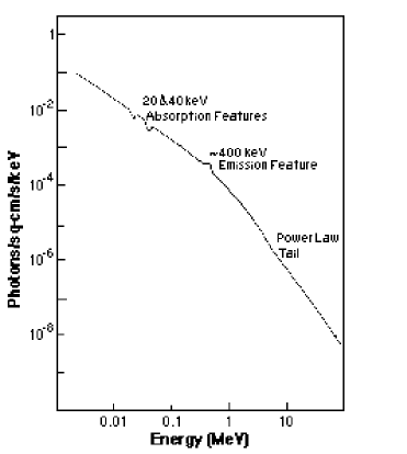
Figure 1.2: Typical energy spectral plot of a gamma-ray burst.

1.1.2 Proposed Models

The actual inner engine that produces the gamma-ray burst is unknown. Researchers speculate that compact objects (black holes, neutron stars, etc.) somehow merge and produce the energy to power a gamma-ray burst. The most widely accepted model appears to be the Fireball model (Piran, 1999) shown in Figure 1.3.

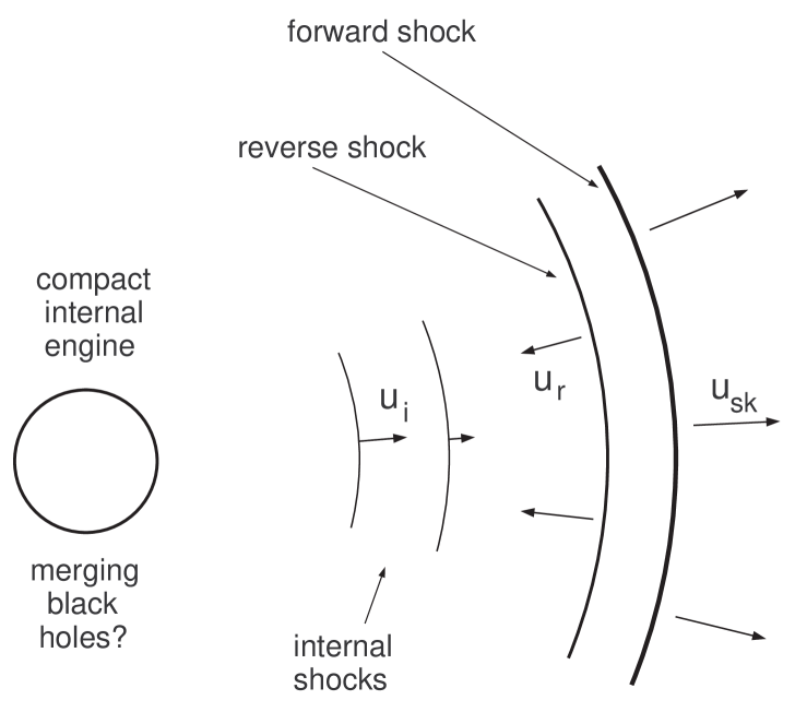
Figure 1.3: The Fireball Model. A highly relativistic (quite likely beamed) forward shock moves outward into the ISM and a reverse shock moves back into the outward moving lepton wind. Various relativistic internal shocks may interact with each other or with the reverse shock to produce intense radiation spikes that make up the initial gamma-ray burst.

By some unknown means, a gamma-ray and/or neutrino radiation-dominated highly relativistic blastwave gives rise to an external shock and an electron-positron pair-dominated ultrarelativistic wind in a region of low baryon density. A reverse shock, traveling backward into the lepton wind, and possibly internal shocks interacting with each other or the reverse shock at slower but still relativistic speeds, may be responsible for the series of intensity peaks seen in the initial gamma-ray burst. The forward shock slows quickly (on the order of minutes) to mildly relativistic speeds as it picks up ambient mass in the interstellar medium. Kinetic energy in the outflow is randomized by magnetic fields, probably collisionless shocks, and is converted back into radiation seen as the afterglow. The computational methods used here allow the study of lepton and baryon dynamics (i.e., Fermi acceleration and the ensuing nonthermal distributions of energetic particles) in the internal shock regions and the external afterglow regions where the shocks speeds have Lorentz factors of 20 or less.

1.2 First order Fermi acceleration

Acceleration of a charged particle as a result of diffusive scattering in converging flows was first suggested by Fermi (1949). There were a number of important papers that developed the concept of diffusive acceleration, or the steady diffusive acceleration of test particles as they cross the shock boundary numerous times and scatter through stochastic processes. Due to the random nature of the scattering process, information is destroyed (i.e., entropy is increased) and the resulting energetic particle distribution is relatively independent of the details of the particle energy distribution prior to acceleration (Drury, 1983). Krymsky (1977), Axford, Leer, & Skadron (1977), and Blandford & Ostriker (1978) used a macroscopic approach to develop an analytical theory of particle acceleration, assuming isotropy in the particle momentum distribution in the fluid frame (because the particle velocity is assumed to be much higher than the fluid velocity), and assuming collisionless, elastic scattering, and assuming the scattering centers are frozen into the background plasma. An accelerated particle momentum spectrum can be generated by using the transport equation in the local fluid frame, and matching boundary conditions for the steady-state solution on each side of the infinite plane shock. This approach is straightforward, but it does not provide an understanding of the physical processes that are responsible for the particle acceleration. A microscopic derivation of diffusive particle acceleration was presented by Bell (1978a), Peacock (1981), and also Michel (1981) which provides much more insight into the physics of the particle acceleration process. A number of papers, Drury (1983), Blandford & Eichler (1987), and Jones & Ellison (1991) among others, review both approaches in detail, covering the effects of oblique magnetic fields, modification of the the shock velocity profile by the backpressure of accelerated particles, and the connection to cosmic rays. The papers cited above deal with nonrelativistic shocks, but they provide a good introduction to shock acceleration of particles.

The most basic concept of nonrelativistic first order Fermi acceleration is shown below. A strong shock wave provides the mechanism by which particles are scattered in pitch angle by magnetic wave turbulence on each side of the shock, as shown in Figure 1.4.

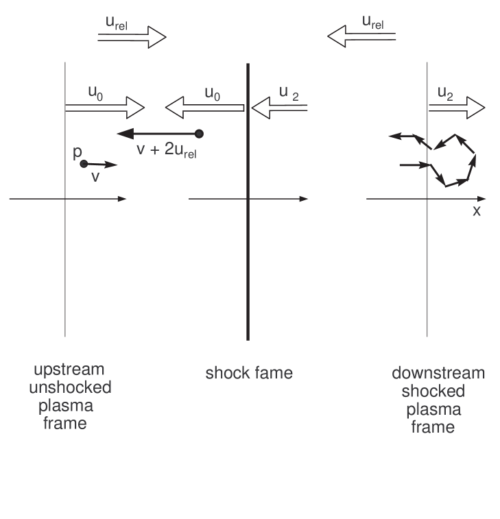
Figure 1.4: Basic conceptional diagram of a plane shock moving through space with a particle scattering elastically in the downstream frame and gaining energy. For nonrelativistic shocks, the upstream and downstream frames converge with relative velocity $u_{\mathrm{rel}}=u_{0}-u_{2}$.

Three frames of reference are shown. The upstream plasma frame sees the shock frame moving toward it with velocity $-u_{0}$ and the downstream frame moving toward it with relative velocity $u_{\mathrm{rel}}=u_{2}-u_{0}$. The shock frame sees the upstream frame as a flow moving toward it with a velocity $+u_{0}$ and the downstream moving away with a velocity $+u_{2}$ The downstream frame sees the upstream frame moving toward it with relative velocity $u_{\mathrm{rel}}=u_{0}-u_{2}$ (i.e., the upstream and downstream frames are converging at a speed $u_{\mathrm{rel}}$) and the downstream frame sees the shock moving away and to the left with a velocity $-u_{2}$. A charged particle, for example a proton, initially at rest in the upstream frame crosses the shock from upstream to downstream because the shock is moving toward it. In the downstream frame, the particle has velocity $+u_{\mathrm{rel}}$. Suppose the particle elastically scatters off of magnetic turbulence in the downstream frame as shown in Figure 1.4 and ends up moving to the left with velocity $-u_{\mathrm{rel}}$. As the particle moves back across the shock, the upstream frame sees the particle, which was originally at rest, now with a velocity of $-2u_{\mathrm{rel}}$ (because the particle had a final velocity of $-u_{\mathrm{rel}}$ in the downstream frame and the downstream frame is moving toward the upstream frame with a velocity of $-u_{\mathrm{rel}}$. Hence, the particle gained in kinetic energy by making a complete passage across the shock and back into the upstream frame. The same argument applies to a particle originally downstream; the particle will also gain the same amount of kinetic energy. By making numerous passages back and forth across the shock, a particle can gain a large amount of kinetic energy, easily becoming relativistic. Obviously, most particles are at some angle with respect to the shock normal, therefore only the $x$ component of the particle’s velocity contributes to the particle’s gain in energy. Since the process is completely random, a distribution of particle energies will result that is independent of the original state of the upstream conditions ((Drury, 1983). In fact, the distribution will result in a power law whose slope depends only on the compression ratio, $r=u_{0}/u_{2}$, between the unshocked, upstream plasma and the shocked downstream plasma, the details of which are discussed at length in the papers cited above.

The main points of the derivation of the power law for accelerated particles are described in a review by Drury (1983). Suppose a particle has momentum $\vec{p}$, velocity $\vec{v}$ and pitch $\mu=\cos(\phi)$ between the momentum vector and the $x$ axis; then the average flux weighted change in a particle’s momentum with respect to the local plasma frame when it crosses the shock is

$$\langle\triangle p\rangle=p\int\limits_{0}^{1}[\mu(u_{0}-u_{2})/v]2\mu d\mu=\frac{2}{3}p(u_{0}-u_{2})/v$$ (1.1)

Therefore, $p_{1}\approx p_{0}[1+\langle\triangle p\rangle]$, and after $N$ shock crossings (or $N/2$ returns from downstream), the average momentum will be

$$\langle p_{N}\rangle=\prod^{N}_{i=1}[1+\frac{2}{3}(u_{0}-u_{2})/v_{i}]p_{0}\approx\prod^{N/2}_{i=1}[1+\frac{4}{3}(u_{0}-u_{2})/v_{i}]p_{0}$$ (1.2)

Then

$$\ln\left[\frac{p_{N}}{p_{0}}\right]=\frac{4}{3}(u_{0}-u_{2})\sum^{N/2}_{i=1}\frac{1}{v_{i}}$$ (1.3)

From the downstream frame, the flux of particles passing through the shock from downstream to upstream is

$$\left|n\int\limits_{-v}^{-u_{2}}(u_{2}+v_{x})dv_{x}\right|=\frac{n}{2}(u_{2}-v)^{2}$$ (1.4)

and the flux of particles passing through the shock from upstream to downstream is

$$n\int\limits_{-u_{2}}^{v}(u_{2}+v_{x})dv_{x}=\frac{n}{2}(u_{2}+v)^{2}$$ (1.5)

The probability of return from downstream to upstream is the ratio of the two fluxes, or

$$P_{R}=\left(\frac{u_{2}-v}{u_{2}+v}\right)^{2}$$ (1.6)

The probability that a particle has returned to the shock at least $N/2$ times is

$$P_{R}(N)=\left[\prod^{N/2}_{i=1}\left(\frac{u_{2}-v_{i}}{u_{2}+v_{i}}\right)\right]^{2}$$ (1.7)

Next, equate summations from the probability equation above and the previous momentum equation:

$$\ln\left[P_{R}(N)\right]=-\frac{3u_{2}}{u_{0}-u_{2}}\ln\left(\frac{p}{p_{0}}\right)$$ (1.8)

This gives the probability that a particle will reach at least momentum $p$:

$$P_{R}(p)=\left(\frac{p}{p_{0}}\right)^{-3u2/(u_{0}-u_{2})}$$ (1.9)

The number density of particles accelerated to momentum p is the product of the initial number density and the probability function:

$$n(p)=P_{R}(N)n(p_{0})=n_{0}\frac{u_{0}}{u_{2}}\left(\frac{p}{p_{0}}\right)^{-3u_{2}/(u_{0}-u_{2})}$$ (1.10)

Finally, the distribution function is

$$f(p)=\frac{1}{4\pi p^{2}}\frac{\partial n}{\partial p}=\frac{n_{o}}{4\pi}\left(\frac{3r}{r-1}\right)\left(\frac{p}{p_{0}}\right)^{-3r/(r-1)}$$ (1.11)

Therefore, with the assumptions of test particles (which leave the plane shock structure unmodified), particle velocities far greater than the nonrelativistic shock velocity and an isotropic distribution of particle momenta, the resulting momentum distribution spectrum depends only on the compression ratio $r$, i.e.,

$$f(p)\propto p^{-\sigma}\qquad\mathrm{where}\qquad\sigma=\hbox{${{\displaystyle 3r\vphantom{(}}\over{\displaystyle r-1\vphantom{(}}}$}$$ (1.12)

Although the derivation of the functional relationship for the momentum distribution with its accompanying assumptions were focused on nonrelativistic shocks, the same concepts of particle acceleration can be applied to relativistic shocks, provided that the new properties which apply to relativistic shocks are taken into account. For example, particle velocities are close to those of the shock velocity (i.e., the speed of light), and this leads to different characteristics and criteria for the particles interacting with the shock. The probability of return equation (1.6) is true in general, even at relativistic speeds, provided the downstream momentum distribution is isotropic, and it should always be found to be isotropic at least one or two mean free paths downstream from the shock. However, the momentum distribution at the shock is highly anisotropic. Particle acceleration by relativistic shocks will be addressed in a later chapter.

1.3 Conservation laws and jump conditions

Particles must obey conservation of momentum, energy and particle continuity across the shock, as well as obey Maxwell’s equations and the thermodynamic equation of state. The nonrelativistic jump conditions are well known; for example, in Ellison, Baring, & Jones (1996), the jump conditions for nonrelativistic shocks with magnetic fields at oblique angles are given in full, and implicitly incorporate the adiabatic equation of state. The jump conditions relate the upstream unshocked plasma to the downstream shocked plasma. Hence, for particles scattering back and forth across the shock, the jump conditions must be satisfied at each crossing and provide a self-consistent solution. This topic will be generalized for relativistic shocks and will be thoroughly discussed in the next two chapters.

1.4 The Monte Carlo approach

Particle acceleration by shocks is inherently complicated and leads to nonlinear differential equations. For example, the compression ratio depends on the adiabatic index, which is affected by the same shock speed that determines the compression ratio (Ellison & Reynolds, 1991). Except for special cases, the macroscopic equations that describe the momentum distributions and jump conditions cannot be solved analytically.

Suppose particle acceleration is viewed microscopically and the individual particles are allowed to scatter kinematically where momentum and energy can be specifically tracked as the particle interacts with the shock environment. This process lends itself nicely to computer techniques, specifically to a Monte Carlo technique developed by Ellison (1981) over the last twenty years and is now a sophisticated tool for analyzing both nonrelativistic and relativistic shocks.

The technique is briefly described here and will be discussed in more detail in a later chapter. The shock region is divided into a number of grid zones, many more than the few shown in Figure 1.5. The model allows a number of particles to be injected into the shock environment far upstream, which simulates unshocked particles in the interstellar medium being subjected to a shock front. As the particles pass through the grid zones, the momentum and energy of the particles are tabulated as corresponding “fluxes”.

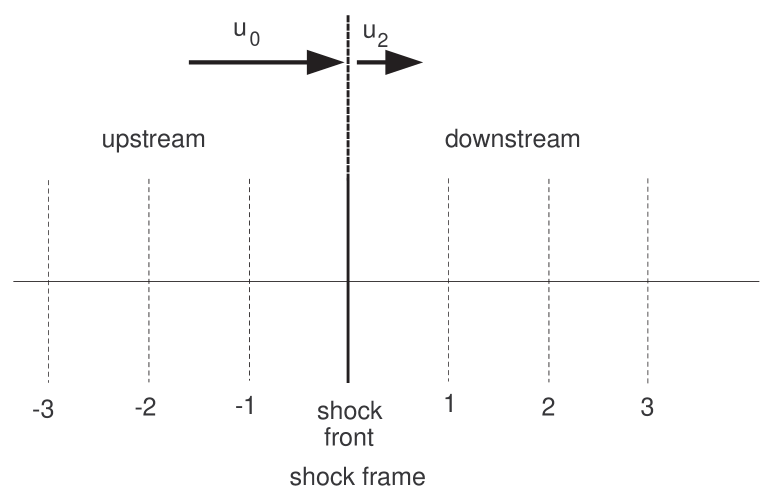
Figure 1.5: The shock environment showing the plasma regions divided up into grid zones for flux calculations by the Monte Carlo model.

In the case of so-called test particles, which do not modify the shock velocity profile, acceleration is turned off in the model, a compression ratio $r=u_{0}/u_{2}$ is chosen and the fluxes are tabulated at all the grid zones, both upstream and downstream. After the particles have completely passed through the shock and if the momentum and energy fluxes vary (i.e., are not conserved) across the shock, then the process is repeated with a different compression ratio until the fluxes appear to show continuity and remain at the same value upstream to downstream.

The Monte Carlo model can also modify the shock velocity profile by allowing the backpressure of accelerated particles to affect the shock in a self-consistent manner. Again, after particles are injected, the Monte Carlo model measures the momentum and energy flux at each grid zone, compares the fluxes to those far upstream and estimates a new shock velocity at each grid zone that may better conserve momentum and energy flux. After a series of iterations, a final shock velocity profile will result that self-consistently conserves momentum and energy flux in the presence of accelerated particles, provided the correct compression ratio was chosen. If the fluxes do not balance across the shock, a new compression ratio is chosen and the process is repeated. Another feature of the model allows the possibility of accelerated particles to escape from the shock, carrying away momentum and energy flux, as discussed in Berezhko & Ellison (1999). These ideas will be discussed more fully in later chapters.

1.5 Overview and Objectives

There are two separate areas of research activity for this dissertation, and they are related in their common objective to understand and explain the observed radiation in gamma-ray bursts.

The first research activity involves the ongoing development of a relativistic nonlinear Monte Carlo model, based on an earlier nonrelativistic version (Ellison, Baring, & Jones, 1996), that will simulate the acceleration of charged particles by relativistic modified shocks with oblique magnetic fields when it is completed. It will be shown that in its current state of development, the model very satisfactorily simulates the collisionless scattering and acceleration of charged particles in relativistic modified shocks with the magnetic field parallel to the normal of the plane of the shock. The development of the model, its operation, and the parameter characteristics for unmodified shocks when shock speed, magnetic field angle and pressure anisotropy are varied, are discussed in Chapters $2$ through $5$. Chapter $2$ explains how and why the stress-energy tensor is used to handle momentum and energy fluxes. The fluid and electromagnetic stress-energy tensors are defined and a new equation of state is developed. The new relativistic magnetohydrodynamic flux relations for momentum and energy are derived in Chapter $3$, along with the new jump conditions across the shock and a new method of estimating the adiabatic index at all shock speeds. Also included in Chapter $3$ is a discussion of some of the compression ratio and magnetic field characteristics for unmodified shocks when the shock speed, magnetic field angle and pressure anisotropy are varied. Chapter $4$ explains the new relativistic momentum transformations between reference frames and how modification of the shock velocity profile by energetic particles occurs. Chapter $5$ describes the Monte Carlo technique for simulating the kinematic scattering and acceleration of particles across a shock front moving at relativistic speeds. An application to parallel, modified shocks is described and the resulting characteristics of the particle distributions, from nonrelativistic to highly relativistic speeds, are discussed.

The second area of research activity utilizes the relativistic shock model to study lepton and baryon acceleration by relativistic modified shocks with the magnetic field parallel to the shock normal. Chapter $6$ provides details of this study where the sensitivity of lepton injection and acceleration to subshock size and shock speed is explored to find the maximum possible energy efficiency of leptons. New results are presented, given the assumptions in this model and if particles are accelerated by diffusive shock acceleration, that suggest leptons can never carry enough energy to explain the observed gamma-ray burst spectra when the lepton to baryon number density is of the same order. Also, the lepton to baryon particle number density ratio is investigated to find the conditions under which leptons can carry the energy needed to produce the radiation observed in gamma-ray bursts. A new result is shown where the equipartition of energy between leptons and baryons is achieved in a relativistic shock when the lepton to baryon number density ratio is approximately $3\times 10^{5}$, independent of shock speed, at least in the range of shock Lorentz factors of $2$ to $12$ used in this study. The results are discussed in the Conclusions in Chapter $7$, along with a summary of all the accomplishments in the two research areas that include the development of the relativistic Monte Carlo model and the lepton-baryon acceleration study.

Chapter 2 The Stress-energy Tensor

The stress-energy tensor describes the condition of a medium at any point in spacetime. One advantage to using a tensor formulation is that it is a very condensed and convenient way to express physical laws. A second advantage, quoting Tolman (1934), “..the expression of a physical law by a tensor equation has exactly the same form in all coordinate systems..”, due to the general transformation rules for tensors; i.e.,

$$T^{\mu\nu...}_{\rho\sigma...}=0$$ (2.1)

will be transformed into an equation of the same form

$$T^{{}^{\prime}\mu\nu...}_{\rho\sigma...}=0$$ (2.2)

when the spacetime coordinates are transformed from $\{x^{1},x^{2},x^{3},x^{4}\}$ to $\{x^{{}^{\prime}1},x^{{}^{\prime}2},x^{{}^{\prime}3},x^{{}^{\prime}4}\}$.

The stress-energy tensor is composed of two primary parts; the fluid tensor and the electromagnetic tensor. Each tensor will be discussed in the sections below. Before discussing these tensors and the corresponding equation of state, some of their components require elaboration.

2.1 The fluid tensor and the equation of state

Aside from the first ($T^{00}$) component of the fluid tensor which is the total energy density in the proper frame, the other stress components of the fluid tensor consist of momenta divided by a unit area. If the normal of the unit area is in the direction of the momenta, the resulting component is called pressure. If the normal of the unit area is perpendicular to the momenta, the resulting component is a shear stress.

Pressure is a macroscopic description of the particle momentum in a given region of space. If the pressure is a scalar quantity, it describes the average momentum or kinetic energy of an ideal fluid in the absence of electromagnetic fields. If the fluid is an ensemble of charged point particles (i.e., a plasma) in the presence of magnetic fields, the pressure may have different values in different directions. In this case, pressure is described by a tensor. In either case, an adiabatic compression or expansion of the region affects the pressure through an adiabatic index. A plasma is dominated by magnetic field effects because the particles move in such a way as to make electric fields negligible. Since a particle’s energy does not ordinarily change by magnetic field deflections (assuming no radiation here), the adiabatic approximation is, in general, a good assumption.

2.1.1 The pressure tensor

Consider a plasma with a magnetic field at some angle $\Theta_{B}$ with respect to the $x$ axis in the $xz$ plane. The pressure tensor will be constrained to the gyrotropic case; i.e., the stress can have one value parallel to the magnetic field vector , but can have a different value perpendicular to the magnetic field vector (with rotational symmetry about the magnetic field vector) as mentioned in equations (B.7) and (B.8). Thus, we have the space tensor

$$\left\{\mathcal{P}^{ij}\right\}_{m}=\left(\begin{array}[]{ccc}P_{\|}&0&0\\ 0&P_{\perp}&0\\ 0&0&P_{\perp}\end{array}\right)$$ (2.3)

where subscript $m$ refers to the magnetic axis coordinate system. Therefore, the pressure-stress tensor is diagonal using the magnetic axis, but rotation from the magnetic field coordinates to the xyz coordinates about the $y$ axis will produce a non-diagonal pressure-stress tensor as described by Ellison, Baring, & Jones (1996). Their 3-dimensional pressure-stress tensor in the xyz plasma frame has components

$$\left\{\mathcal{P}^{ij}\right\}_{p}=\left(\begin{array}[]{ccc}P_{\|}\cos^{2}{\Theta_{B}}+P_{\perp}\sin^{2}{\Theta_{B}}&0&(P_{\perp}-P_{\|})\sin{\Theta_{B}}\cos{\Theta_{B}}\\ 0&P_{\perp}&0\\ (P_{\perp}-P_{\|})\sin{\Theta_{B}}\cos{\Theta_{B}}&0&P_{\perp}\cos^{2}{\Theta_{B}}+P_{\|}\sin^{2}{\Theta_{B}}\end{array}\right)$$ (2.4)

corresponding to

$$\left\{\mathcal{P}^{ij}\right\}_{p}=\left(\begin{array}[]{ccc}P_{xx}&0&P_{xz}\\ 0&P_{yy}&0\\ P_{zx}&0&P_{zz}\end{array}\right)$$ (2.5)

where

$$P_{\parallel}=P_{xx}-P_{xz}\hbox{${{\displaystyle\sin{\Theta_{B}}\vphantom{(}}\over{\displaystyle\cos{\Theta_{B}}\vphantom{(}}}$}$$ (2.6)

and

$$P_{\perp}=P_{xx}+P_{xz}\hbox{${{\displaystyle\cos{\Theta_{B}}\vphantom{(}}\over{\displaystyle\sin{\Theta_{B}}\vphantom{(}}}$}$$ (2.7)

The third equation completes the set:

$$P_{zz}=P_{xx}+P_{xz}\left(\hbox{${{\displaystyle\cos^{2}{\Theta_{B}}-\sin^{2}{\Theta_{B}}\vphantom{(}}\over{\displaystyle\sin{\Theta_{B}}\cos{\Theta_{B}}\vphantom{(}}}$}\right)=P_{xx}+2P_{xz}\cot{(2\Theta_{B})}$$ (2.8)

2.1.2 The fluid stress-energy tensor

The fluid stress-energy tensor in the proper frame is defined with the following corresponding components:

$$T^{\mu\nu}_{fluid}=\left(\begin{array}[]{cccc}e&0&0&0\\[2.84544pt] 0&P_{xx}&0&P_{xz}\\[5.69046pt] 0&0&P_{yy}&0\\[5.69046pt] 0&P_{zx}&0&P_{zz}\end{array}\right)$$ (2.9)

using $P_{xx}$, $P_{zz}$ and $P_{xz}=P_{zx}$ from the previous section.

The $T^{00}$ component, $e$, is the total energy density in the proper frame or plasma frame. The other components $P_{ij}$ are defined by Tolman (1934) as the “absolute stress” components in the proper frame. $P_{ij}$ is the force parallel to the $i$-axis exerted on a unit area normal to the $j$-axis. Hence, the diagonal components can be considered a pressure, but the off-axis components are shear stresses. The absolute stress components represent a different physical concept than the thermodynamic scalar pressure $P$. Scalar pressure $P$ assumes a Maxwell-Boltzmann distribution and is Lorentz invariant. The non-thermal components of the pressure-stress tensor $\mathcal{P}^{ij}$ embodied in the fluid tensor above, in general, transform significantly and pick up momentum flux components in reference frames moving with respect to the proper frame. It may be noted that at nonrelativistic speeds, the pressure-stress tensor is invariant under Galilean transformations because force and area are invariant.

A general adiabatic equation of state can be created from the conservation of energy density when oblique magnetic fields are present:

$$e=\hbox{${{\displaystyle Tr\{P_{ij}\}\vphantom{(}}\over{\displaystyle 3(\Gamma-1)\vphantom{(}}}$}+\rho c^{2}$$ (2.10)

where the trace of the pressure-stress tensor is $Tr\{\mathcal{P}^{ij}\}=P_{\|}+2P_{\perp}$, $\Gamma$ is the adiabatic index, and $\rho$ is the rest mass density. Using equations (2.6) and (2.7) one can write

$$\hbox{${{\displaystyle Tr\{\mathcal{P}^{ij}\}\vphantom{(}}\over{\displaystyle 3(\Gamma-1)\vphantom{(}}}$}=\hbox{${{\displaystyle 1\vphantom{(}}\over{\displaystyle 3(\Gamma-1)\vphantom{(}}}$}(P_{\parallel}+2P_{\perp})=\hbox{${{\displaystyle 1\vphantom{(}}\over{\displaystyle\Gamma-1\vphantom{(}}}$}\left[P_{xx}+\hbox{${{\displaystyle P_{xz}\vphantom{(}}\over{\displaystyle 3\vphantom{(}}}$}\left(2\cot{\Theta}-\tan{\Theta}\right)\right]\ .$$ (2.11)

In terms of magnetic field, where $\cot\Theta_{B}=\hbox{${{\displaystyle B_{x}\vphantom{(}}\over{\displaystyle B_{z}\vphantom{(}}}$}$ and $\tan\Theta_{B}=\hbox{${{\displaystyle B_{z}\vphantom{(}}\over{\displaystyle B_{x}\vphantom{(}}}$}$, this becomes

$$\hbox{${{\displaystyle 1\vphantom{(}}\over{\displaystyle 3(\Gamma-1)\vphantom{(}}}$}(P_{\parallel}+2P_{\perp})=\hbox{${{\displaystyle 1\vphantom{(}}\over{\displaystyle\Gamma-1\vphantom{(}}}$}\left[P_{xx}+\hbox{${{\displaystyle P_{xz}\vphantom{(}}\over{\displaystyle 3\vphantom{(}}}$}\left(2\hbox{${{\displaystyle B_{x}\vphantom{(}}\over{\displaystyle B_{z}\vphantom{(}}}$}-\hbox{${{\displaystyle B_{z}\vphantom{(}}\over{\displaystyle B_{x}\vphantom{(}}}$}\right)\right]\ .$$ (2.12)

Hence, the adiabatic equation of state, valid for both relativistic and nonrelativistic shocks, is

$$e=\hbox{${{\displaystyle 1\vphantom{(}}\over{\displaystyle\Gamma-1\vphantom{(}}}$}\left[P_{xx}+\hbox{${{\displaystyle P_{xz}\vphantom{(}}\over{\displaystyle 3\vphantom{(}}}$}\left(2\hbox{${{\displaystyle B_{x}\vphantom{(}}\over{\displaystyle B_{z}\vphantom{(}}}$}-\hbox{${{\displaystyle B_{z}\vphantom{(}}\over{\displaystyle B_{x}\vphantom{(}}}$}\right)\right]+\rho c^{2}\ .$$ (2.13)

2.1.3 Scalar pressure

Scalar pressure is isotropic and Lorentz invariant. It is based on either the ideal gas law $P=nkT$ where $k$ is Boltzmann’s constant, or it is calculated by averaging the squares of the individual particle momenta. When scalar pressure is presented as a three dimensional tensor, it is diagonal with equal components in all reference frames. The simplified equation of state, discussed in Appendix B, is stated again here:

$$e=\hbox{${{\displaystyle P\vphantom{(}}\over{\displaystyle\Gamma-1\vphantom{(}}}$}+\rho c^{2}\ .$$ (2.14)

The fluid tensor in the plasma frame becomes

$$T^{\mu\nu}_{fluid}=\left(\begin{array}[]{cccc}e&0&0&0\\ 0&P&0&0\\ 0&0&P&0\\ 0&0&0&P\end{array}\right).$$ (2.15)

2.2 The Electromagnetic Stress-energy Tensor

The electromagnetic field tensor composed by Landau & Lifshitz (1962) or the equivalent field-strength tensor of Jackson (1975), each effectively using the Lorentz gauge, can be stated as

$$F^{\mu\nu}=\left(\begin{array}[]{cccc}0&-E_{x}&-E_{y}&-E_{z}\\ E_{x}&0&-B_{z}&B_{y}\\ E_{y}&B_{z}&0&-B_{x}\\ E_{z}&-B_{y}&B_{x}&0\end{array}\right)$$ (2.16)

and it’s dual,

$$\mathcal{F}^{\mu\nu}=\left(\begin{array}[]{cccc}0&-B_{x}&-B_{y}&-B_{z}\\ B_{x}&0&E_{z}&-E_{y}\\ B_{y}&-E_{z}&0&E_{x}\\ B_{z}&E_{y}&-E_{x}&0\end{array}\right)$$ (2.17)

and from these field-strength tensors, the covariant form of the inhomogeneous Maxwell equations may be written as

$$F_{,\mu}^{\mu\nu}=\hbox{${{\displaystyle 4\pi\vphantom{(}}\over{\displaystyle c\vphantom{(}}}$}J^{\nu}$$ (2.18)

and the homogeneous equations may be written as

$$\mathcal{F}_{,\mu}^{\mu\nu}=0$$ (2.19)

accompanied by the continuity equation

$$J_{,\mu}^{\nu}=0$$ (2.20)

where $J^{\nu}=(c\rho_{q},\vec{J})$ is the current four-vector, $\vec{J}$ is the current density three-space vector, and $\rho_{q}$ is the electric charge density.

However, what is actually required is the electromagnetic energy momentum tensor or electromagnetic stress-energy tensor. This tensor can be constructed from the field tensors above as, for example, Appl & Camenzind (1988) did, but referring to Tolman (1934), the electromagnetic stress-energy tensor may be written directly as

$$T^{\mu\nu}_{\mathrm{EM}}=\hbox{${{\displaystyle 1\vphantom{(}}\over{\displaystyle 4\pi\vphantom{(}}}$}\left(\begin{array}[]{cccc}\hbox{${{\displaystyle E^{2}+B^{2}\vphantom{(}}\over{\displaystyle 2\vphantom{(}}}$}&\left[\vec{E}\times\vec{B}\right]_{x}&\left[\vec{E}\times\vec{B}\right]_{y}&\left[\vec{E}\times\vec{B}\right]_{z}\\[5.69046pt] \left[\vec{E}\times\vec{B}\right]_{x}&Q_{xx}&Q_{xy}&Q_{xz}\\[8.5359pt] \left[\vec{E}\times\vec{B}\right]_{y}&Q_{yx}&Q_{yy}&Q_{yz}\\[8.5359pt] \left[\vec{E}\times\vec{B}\right]_{z}&Q_{zx}&Q_{zy}&Q_{zz}\end{array}\right)$$ (2.21)

where the Q’s are the Maxwell stresses defined as:

$$Q_{ii}=\hbox{${{\displaystyle E^{2}+B^{2}\vphantom{(}}\over{\displaystyle 2\vphantom{(}}}$}-E^{2}_{i}-B^{2}_{i}\quad\mathrm{and}\quad Q_{ij}=-(E_{i}E_{j}+B_{i}B_{j})$$ (2.22)

The overall electric field in a plasma is negligible and the plasma is dominated by magnetic fields. In addition, the $xyz$ coordinate system is oriented such that the magnetic field lies in the $xz$ plane; hence, the electromagnetic stress-energy tensor can be simplified to

$$T^{\mu\nu}_{\mathrm{EM}}=\hbox{${{\displaystyle 1\vphantom{(}}\over{\displaystyle 4\pi\vphantom{(}}}$}\left(\begin{array}[]{cccc}\hbox{${{\displaystyle B^{2}\vphantom{(}}\over{\displaystyle 2\vphantom{(}}}$}&0&0&0\\ 0&\hbox{${{\displaystyle B^{2}_{z}-B^{2}_{x}\vphantom{(}}\over{\displaystyle 2\vphantom{(}}}$}&0&-B_{x}B_{z}\\ 0&0&\hbox{${{\displaystyle B^{2}\vphantom{(}}\over{\displaystyle 2\vphantom{(}}}$}&0\\ 0&-B_{z}B_{x}&0&\hbox{${{\displaystyle B^{2}_{x}-B^{2}_{z}\vphantom{(}}\over{\displaystyle 2\vphantom{(}}}$}\end{array}\right)\ .$$ (2.23)

2.3 Summary

The concept of the stress-energy tensor was presented, and why and how it is used to handle momentum and energy fluxes, both fluid and electromagnetic, in the Monte Carlo relativistic shock model. The stress-energy tensor was shown to consist of two parts. The first part contains total fluid energy and a gyrotropic pressure tensor. The second part contains magnetic fields, with the assumption that electric fields, over the large scale, are negligible in the space plasma. From these tensors a new equation of state was established that is valid for both nonrelativistic and relativistic shocks. The equation of state includes a gyrotropic pressure tensor and oblique magnetic fields.

Chapter 3 Relativistic Magnetohydrodynamic Jump Conditions

Relativistic shock jump conditions have been presented in a variety of ways over the years. The standard technique for deriving the equations is to set the divergence of the stress-energy tensor equal to zero on a thin volume enclosing the shock plane and use Gauss’s theorem to generate the jump conditions across the shock. For example, Taub (1948) developed the relativistic form of the Rankine-Hugoniot relations, using the stress-energy tensor with velocity expressed in terms of the Maxwell-Boltzmann distribution function for a simple gas. de Hoffmann & Teller (1950) presented a relativistic MHD treatment of shocks in various orientations and a treatment of oblique shocks for the nonrelativistic case, eliminating the electric field by transforming to a frame where the flow velocity is parallel to the magnetic field vector (now called the de Hoffmann-Teller frame). Peacock (1981), following Landau & Lifshitz (1959), presented jump conditions without electromagnetic fields, and Blandford & McKee (1976), also using the approach of Landau & Lifshitz (1959) and Taub (1948), developed a concise set of jump conditions for a simple gas using scalar pressure. Webb, Zank & McKenzie (1987) provided a review of relativistic MHD shocks in ideal, perfectly conducting plasmas, and in particular the treatment by Lichnerowicz (1967, 1970), which used this approach to develop the relativistic analog of Cabannes’ shock polar (Cabannes, 1970) whose origins also lie in Landau & Lifshitz (1959). Kirk & Webb (1988) developed hydrodynamic equations using a pressure tensor, and Appl & Camenzind (1988) developed relativistic shock equations for MHD jets using scalar pressure and magnetic fields with components $B_{z}$ and $B_{\phi}$ (a parallel field with a twist). Ballard & Heavens (1991) derived MHD jump conditions using the stress-energy tensor with isotropic pressure and the Maxwell field tensor. By using a Lorentz transformation to the de Hoffman-Teller frame, they restricted shock speeds, $u_{0}$, to $u_{0}/c<\cos{\Theta_{\mathrm{Bn}}}$, where $\Theta_{\mathrm{Bn}}$ is the angle between the shock normal and the upstream magnetic field; hence, this approach may only be used for mildly relativistic applications. All of these approaches assumed that particles encountered by the shock did not affect the shock velocity profile, i.e., shocked particles were treated as test particles.

Here, previous work is extended by deriving a set of fully relativistic MHD jump conditions with gyrotropic pressure and oblique magnetic fields. The results are not restricted to the de Hoffmann-Teller frame and apply for arbitrary shock speeds and arbitrary shock obliquities. Solutions to the equations determine the downstream state of the gas in terms of the upstream state for the special case of isotropic pressure and, by parameterizing the pressure parallel and perpendicular to the magnetic field, for gyrotropic pressure. In this chapter analytic methods are used for determining the fluid and electromagnetic characteristics of the shock and do not include particle acceleration. Later work will combine these results with Monte Carlo techniques (e.g., Ellison, Baring, & Jones, 1996; Ellison & Double, 2002) that will allow the modeling of diffusive particle acceleration, including the modification of the shock structure resulting from the back-reaction of energetic particles on the upstream flow.

3.1 Derivation of MHD jump conditions

3.1.1 Steady-state, plane shock

Utilizing a Cartesian coordinate system with the $+x$-axis pointing to the right, an infinite, steady-state, plane shock is shown in Figure 3.1 traveling to the left at a speed $u_{0}$ with it’s velocity vector parallel to the normal of the plane of the shock. In the rest frame of the shock, the upstream fluid appears to be flowing to the right with a speed of $u_{0}$.

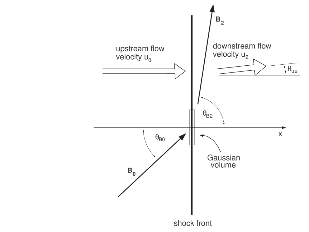
Figure 3.1: Schematic diagram of a plane shock, in the rest frame of the shock, showing oblique magnetic fields and a Gaussian volume over which the divergence of the stress-energy tensor is integrated. In all of the examples the upstream flow is parallel to the shock normal.

The upstream unshocked fluid consists of a tenuous, plasma of baryons and leptons in thermal equilibrium with $\mathcal{T}_{p0}=\mathcal{T}_{e0}$, where $\mathcal{T}_{p0}$ ($\mathcal{T}_{e0}$) is the baryon (lepton) temperature. A uniform magnetic field, $B$, makes an angle $\Theta_{\mathrm{B0}}$ with respect to the $x$-axis as seen from the upstream plasma frame. The field is kept weak enough to insure high Alfvén Mach numbers and thus to insure that the magnetic turbulence responsible for scattering the particles is frozen into the plasma. The $xyz$ coordinate system is oriented such that there are only two components of magnetic field, $B_{x0}$ and $B_{z0}$, in the upstream frame. The field will remain co-planar in the downstream frame and the downstream flow speed will be confined to the $x$-$z$ plane as well (e.g., Jones & Ellison, 1987).

In the shock frame, the upstream flow is in the $+x$-direction and is described by the normalized velocity four-vector $\beta^{\nu}_{0}=\gamma_{0}(1,\beta_{0}^{x},0,0)$. The downstream (i.e., shocked) flow velocity four-vector is $\beta^{\nu}_{2}=\gamma_{2}(1,\beta_{2}^{x},0,\beta_{2}^{z})$, where the subscript 0 (2) refers, here and elsewhere, to upstream (downstream) quantities, $\beta=u/c$, and $\gamma=(1-\beta^{2})^{-1/2}$ is the corresponding Lorentz factor associated with the magnitude of the flow velocity, $u$.

The set of equations connecting the upstream and downstream regions of a shock consist of the continuity of particle number flux (for conserved particles), momentum and energy flux conservation, plus electromagnetic boundary conditions at the shock interface, and the equation of state. The various parameters that define the state of the plasma, such as pressure and magnetic field, are determined in the plasma frame and must be Lorentz transformed to the shock frame where the jump conditions apply. In general, the six jump conditions plus the equation of state cannot be solved analytically because the adiabatic index (i.e., the ratio of specific heats in the nonrelativistic and ultrarelativistic limits) is a function of the downstream plasma parameters, creating an inherently nonlinear problem (e.g., Ellison & Reynolds, 1991). Even with the assumption of gyrotropic pressure, there are more unknowns than there are equations; however, with additional assumptions, approximate analytic solutions may be obtained.

3.1.2 Transformation Properties of the Stress-Energy Tensor

Following Tolman (1934), equations (2.9) and (2.23) are combined to create the total stress-energy tensor, $T^{\mu\nu}_{\mathrm{total}}$, as the sum of fluid and electromagnetic parts, i.e.,

$$T^{\mu\nu}_{\mathrm{total}}=T^{\mu\nu}_{\mathrm{fluid}}+T^{\mu\nu}_{\mathrm{EM}}\ .$$ (3.1)

Then, by integrating over a thin volume containing the shock plane as shown in Figure 3.1 and, with Gauss’ theorem, obtain the energy and momentum flux conditions across the plane of the shock by using $T^{\mu\nu}n_{\nu}=0$. Thus, it can be seen that $T^{0\nu}n_{\nu}$ yields the conservation of energy flux, $T^{1\nu}n_{\nu}$ yields the $x$-contribution to momentum flux conservation in the $x$-direction, $T^{3\nu}n_{\nu}$ yields the $z$-contribution to momentum flux conservation in the $x$-direction, and $n_{\nu}=(0,1,0,0)$ is the unit four-vector along the $x$-axis in the reference frame of the shock. The Einstein summation convention is used here and throughout this thesis; Repeated Greek indices are summed over four-space(time) and repeated English indices are summed over three-space.

The components of the fluid and electromagnetic tensors are defined in the local plasma frame and are Lorentz transformed to the shock frame where the flux conservation conditions apply, i.e.,

$$\left\{T^{\mu\nu}_{\mathrm{total}}\right\}_{s}=\Lambda^{\mu}_{\alpha}\left[\left\{T_{\mathrm{fluid}}^{\alpha\beta}\right\}_{p}+\left\{T^{\alpha\beta}_{\mathrm{EM}}\right\}_{p}\right]\Lambda^{\nu}_{\beta}\ ,$$ (3.2)

where the subscript $p$ ($s$) refers to the plasma (shock) frame. Since the flow speeds in the model may have two space components, in the $x$ and $z$-directions, the Lorentz transformation is

$$\Lambda^{\mu}_{\alpha}=\left(\begin{array}[]{cccc}\gamma&\gamma\beta_{x}&0&\gamma\beta_{z}\\[8.5359pt] \gamma\beta_{x}&1+\hbox{${{\displaystyle\gamma-1\vphantom{(}}\over{\displaystyle\beta^{2}\vphantom{(}}}$}\beta_{x}^{2}&0&\hbox{${{\displaystyle\gamma-1\vphantom{(}}\over{\displaystyle\beta^{2}\vphantom{(}}}$}\beta_{x}\beta_{z}\\[11.38092pt] 0&0&1&0\\[11.38092pt] \gamma\beta_{z}&\hbox{${{\displaystyle\gamma-1\vphantom{(}}\over{\displaystyle\beta^{2}\vphantom{(}}}$}\beta_{z}\beta_{x}&0&1+\hbox{${{\displaystyle\gamma-1\vphantom{(}}\over{\displaystyle\beta^{2}\vphantom{(}}}$}\beta_{z}^{2}\end{array}\right)$$ (3.3)

where $\gamma=(1-\beta^{2})^{-\frac{1}{2}}$, $\beta^{2}=\beta^{i}\beta_{i}$ is the square of the normalized flow speed as seen from the shock frame, and $i$ is summed over the space components.

3.1.3 Flux Conservation Relations

As discussed above, the energy and momentum conservation relations in the shock frame can be derived by applying $T^{\mu\nu}n_{\nu}=0$ to equation (3.2), individually on the Lorentz transformed fluid and electromagnetic tensors.

The conservation of energy flux derives from

$$\left\{T^{0\nu}_{\mathrm{total}}\right\}_{s}n_{\nu}=\left\{T^{0\nu}_{\mathrm{fluid}}\right\}_{s}n_{\nu}+\left\{T^{0\nu}_{\mathrm{EM}}\right\}_{s}n_{\nu}=0\ .$$ (3.4)

The fluid contribution to energy (scalar) flux conservation is

$$F^{\mathrm{fluid}}_{en}=\left\{T^{0\nu}_{\mathrm{fluid}}\right\}_{s}n_{\nu}=\gamma^{2}\beta_{x}(e+P_{xx})-\gamma(\gamma-1)\hbox{${{\displaystyle\beta_{x}\beta_{z}^{2}\vphantom{(}}\over{\displaystyle\beta^{2}\vphantom{(}}}$}(P_{xx}-P_{zz})+\hskip 71.13188pt$$

$$\gamma\left[(2\gamma-1)\beta_{x}^{2}+\beta_{z}^{2}\right]\hbox{${{\displaystyle\beta_{z}\vphantom{(}}\over{\displaystyle\beta^{2}\vphantom{(}}}$}P_{xz}\ ,\hskip 28.45274pt$$ (3.5)

while the electromagnetic contribution is

$$F^{\mathrm{EM}}_{en}=\left\{T^{0\nu}_{\mathrm{EM}}\right\}_{s}n_{\nu}=\hbox{${{\displaystyle\gamma\vphantom{(}}\over{\displaystyle 4\pi\beta^{2}\vphantom{(}}}$}\left[(\gamma-1)\beta_{x}\beta_{z}^{2}B_{x}^{2}+(\gamma\beta_{x}^{2}+\beta_{z}^{2})\beta_{x}B_{z}^{2}-\hskip 79.6678pt\right.$$

$$\left.\{(2\gamma-1)\beta_{x}^{2}+\beta_{z}^{2}\}\beta_{z}B_{x}B_{z}\right]\ .\hskip 14.22636pt$$ (3.6)

The conservation of momentum flux derives from

$$\left\{T^{i\nu}_{\mathrm{total}}\right\}_{s}n_{\nu}=\left\{T^{i\nu}_{\mathrm{fluid}}\right\}_{s}n_{\nu}+\left\{T^{i\nu}_{\mathrm{EM}}\right\}_{s}n_{\nu}=0\ .$$ (3.7)

The $x$-component of the fluid tensor contributing to momentum flux is

$$F^{\mathrm{fluid}}_{px}=\left\{T^{1\nu}_{\mathrm{fluid}}\right\}_{s}n_{\nu}=\gamma^{2}\beta_{x}^{2}(e+P_{xx})+P_{xx}-(\gamma-1)^{2}\hbox{${{\displaystyle\beta_{x}^{2}\beta_{z}^{2}\vphantom{(}}\over{\displaystyle\beta^{4}\vphantom{(}}}$}(P_{xx}-P_{zz})+\hskip 28.45274pt$$

$$2(\gamma-1)(\gamma\beta_{x}^{2}+\beta_{z}^{2})\hbox{${{\displaystyle\beta_{x}\beta_{z}\vphantom{(}}\over{\displaystyle\beta^{4}\vphantom{(}}}$}P_{xz}\ ,\hskip 28.45274pt$$ (3.8)

and the $z$-component is

$$F^{\mathrm{fluid}}_{pz}=\left\{T^{3\nu}_{\mathrm{fluid}}\right\}_{s}n_{\nu}=\gamma^{2}\beta_{x}\beta_{z}(e+P_{xx})-(\gamma-1)(\beta_{x}^{2}+\gamma\beta_{z}^{2})\hbox{${{\displaystyle\beta_{x}\beta_{z}\vphantom{(}}\over{\displaystyle\beta^{4}\vphantom{(}}}$}(P_{xx}-P_{zz})+\qquad\qquad$$

$$\left[\gamma+2(\gamma-1)^{2}\hbox{${{\displaystyle\beta_{x}^{2}\beta_{z}^{2}\vphantom{(}}\over{\displaystyle\beta^{4}\vphantom{(}}}$}\right]P_{xz}\ .\hskip 28.45274pt$$ (3.9)

The $x$-component of the electromagnetic tensor contributing to momentum flux is

$$F^{\mathrm{EM}}_{px}=\left\{T^{1\nu}_{\mathrm{EM}}\right\}_{s}n_{\nu}=\hbox{${{\displaystyle\gamma^{2}\vphantom{(}}\over{\displaystyle 8\pi\vphantom{(}}}$}\beta_{x}^{2}B^{2}+\hbox{${{\displaystyle 1\vphantom{(}}\over{\displaystyle 8\pi\beta^{4}\vphantom{(}}}$}\left[(\gamma\beta_{x}^{2}+\beta_{z}^{2})^{2}-(\gamma-1)^{2}\beta_{x}^{2}\beta_{z}^{2}\right](B_{z}^{2}-B_{x}^{2})-\hskip 28.45274pt$$

$$\hbox{${{\displaystyle 1\vphantom{(}}\over{\displaystyle 2\pi\vphantom{(}}}$}(\gamma-1)(\gamma\beta_{x}^{2}+\beta_{z}^{2})\hbox{${{\displaystyle\beta_{x}\beta_{z}\vphantom{(}}\over{\displaystyle\beta^{4}\vphantom{(}}}$}B_{x}B_{z}\ ,\hskip 22.76228pt$$ (3.10)

and the $z$-component is

$$F^{\mathrm{EM}}_{pz}=\left\{T^{3\nu}_{\mathrm{EM}}\right\}_{s}n_{\nu}=\hbox{${{\displaystyle\gamma^{2}\vphantom{(}}\over{\displaystyle 8\pi\vphantom{(}}}$}\beta_{x}\beta_{z}B^{2}+\hbox{${{\displaystyle 1\vphantom{(}}\over{\displaystyle 8\pi\vphantom{(}}}$}(\gamma-1)^{2}(\beta_{x}^{2}-\beta_{z}^{2})\hbox{${{\displaystyle\beta_{x}\beta_{z}\vphantom{(}}\over{\displaystyle\beta^{4}\vphantom{(}}}$}(B_{z}^{2}-B_{x}^{2})-\hskip 56.9055pt$$

$$\hbox{${{\displaystyle 1\vphantom{(}}\over{\displaystyle 2\pi\vphantom{(}}}$}(\gamma-1)^{2}\hbox{${{\displaystyle\beta_{x}^{2}\beta_{z}^{2}\vphantom{(}}\over{\displaystyle\beta^{4}\vphantom{(}}}$}B_{x}B_{z}-\hbox{${{\displaystyle\gamma\vphantom{(}}\over{\displaystyle 4\pi\vphantom{(}}}$}B_{x}B_{z}\ .\hskip 28.45274pt$$ (3.11)

In all cases where the Alfvén Mach number is large, the downstream flow velocity deviates only slightly from the shock normal direction so $\beta_{z}\ll\beta_{x}$ as shown in the bottom frame of Figure 3.2. This allows a first-order approximation in $\beta_{z}$ and the above equations become:

$$F^{\mathrm{fluid}}_{en}\approx\gamma^{2}\beta_{x}(e+P_{xx})+\gamma(2\gamma-1)\beta_{z}P_{xz}\ ,$$ (3.12)

$$F^{\mathrm{EM}}_{en}\approx\hbox{${{\displaystyle\gamma^{2}\vphantom{(}}\over{\displaystyle 4\pi\vphantom{(}}}$}\beta_{x}B_{z}^{2}-\hbox{${{\displaystyle\gamma\vphantom{(}}\over{\displaystyle 4\pi\vphantom{(}}}$}(2\gamma-1)\beta_{z}B_{x}B_{z}\ ,$$ (3.13)

$$F^{\mathrm{fluid}}_{px}\approx\gamma^{2}\beta_{x}^{2}(e+P_{xx})+P_{xx}+2\gamma(\gamma-1)\hbox{${{\displaystyle\beta_{z}\vphantom{(}}\over{\displaystyle\beta_{x}\vphantom{(}}}$}P_{xz}\ ,$$ (3.14)

$$F^{\mathrm{EM}}_{px}\approx\hbox{${{\displaystyle\gamma^{2}\vphantom{(}}\over{\displaystyle 8\pi\vphantom{(}}}$}\beta_{x}^{2}B^{2}+\hbox{${{\displaystyle\gamma^{2}\vphantom{(}}\over{\displaystyle 8\pi\vphantom{(}}}$}(B_{z}^{2}-B_{x}^{2})-\hbox{${{\displaystyle\gamma(\gamma-1)\vphantom{(}}\over{\displaystyle 2\pi\vphantom{(}}}$}\hbox{${{\displaystyle\beta_{z}\vphantom{(}}\over{\displaystyle\beta_{x}\vphantom{(}}}$}B_{x}B_{z}\ ,$$ (3.15)

$$F^{\mathrm{fluid}}_{pz}\approx\gamma^{2}\beta_{x}\beta_{z}(e+P_{xx})+\gamma P_{xz}-(\gamma-1)\hbox{${{\displaystyle\beta_{z}\vphantom{(}}\over{\displaystyle\beta_{x}\vphantom{(}}}$}(P_{xx}-P_{zz})\ ,$$ (3.16)

and

$$F^{\mathrm{EM}}_{pz}\approx\hbox{${{\displaystyle\gamma^{2}\vphantom{(}}\over{\displaystyle 8\pi\vphantom{(}}}$}\beta_{x}\beta_{z}B^{2}+\hbox{${{\displaystyle 1\vphantom{(}}\over{\displaystyle 8\pi\vphantom{(}}}$}(\gamma-1)^{2}\hbox{${{\displaystyle\beta_{z}\vphantom{(}}\over{\displaystyle\beta_{x}\vphantom{(}}}$}(B_{z}^{2}-B_{x}^{2})-\hbox{${{\displaystyle\gamma\vphantom{(}}\over{\displaystyle 4\pi\vphantom{(}}}$}B_{x}B_{z}\ .$$ (3.17)

As shown in the bottom frame of Figure 3.3, the approximation $\beta_{z}\ll\beta_{x}$ becomes progressively better as the shock Lorentz factor increases.

When the shock speed is ultrarelativistic, or when the magnetic field is parallel to the shock normal, $\beta_{z}=0$ and the above equations can be simplified further.

For the ultrarelativistic case:

$$F^{\mathrm{fluid}}_{en}=\gamma^{2}\beta_{x}(e+P_{xx})\ ,$$ (3.18)

$$F^{\mathrm{EM}}_{en}=\hbox{${{\displaystyle\gamma^{2}\vphantom{(}}\over{\displaystyle 4\pi\vphantom{(}}}$}\beta_{x}B_{z}^{2}\ ,$$ (3.19)

$$F^{\mathrm{fluid}}_{px}=\gamma^{2}\beta_{x}^{2}(e+P_{xx})\ ,$$ (3.20)

$$F^{\mathrm{EM}}_{px}=\hbox{${{\displaystyle\gamma^{2}\vphantom{(}}\over{\displaystyle 4\pi\vphantom{(}}}$}B_{z}^{2}$$ (3.21)

$$F^{\mathrm{fluid}}_{pz}=\gamma P_{xz}\ ,$$ (3.22)

and

$$F^{\mathrm{EM}}_{pz}=-\hbox{${{\displaystyle\gamma\vphantom{(}}\over{\displaystyle 4\pi\vphantom{(}}}$}B_{x}B_{z}\ .$$ (3.23)

For parallel fields:

$$F^{\mathrm{fluid}}_{en}=\gamma^{2}\beta_{x}(e+P_{xx})\ ,$$ (3.24)

$$F^{\mathrm{EM}}_{en}=0\ ,$$ (3.25)

$$F^{\mathrm{fluid}}_{px}=\gamma^{2}\beta_{x}^{2}(e+P_{xx})+P_{xx}\ ,$$ (3.26)

$$F^{\mathrm{EM}}_{px}=0\ ,$$ (3.27)

$$F^{\mathrm{fluid}}_{pz}=0\ ,$$ (3.28)

and

$$F^{\mathrm{EM}}_{pz}=0$$ (3.29)

.

3.1.4 Jump conditions

The jump conditions consist of the energy and momentum flux conservation relations, the particle flux continuity, and the boundary conditions on the magnetic field. The conservation of particle number flux is

$$\bigg{[}\gamma n\beta_{x}\bigg{]}^{2}_{0}=0\ ,$$ (3.30)

where the brackets are used as an abbreviation for

$$\gamma_{2}n_{2}\beta_{x2}-\gamma_{0}n_{0}\beta_{x0}=0\ .$$ (3.31)

This jump condition, as well as the ones that follow, are written in the shock frame and, as always, the subscript 0 (2) refers to upstream (downstream) quantities. The remaining jump conditions are:

$$\bigg{[}F^{\mathrm{fluid}}_{en}+F^{\mathrm{EM}}_{en}\bigg{]}^{2}_{0}=0\ ,$$ (3.32)

$$\bigg{[}F^{\mathrm{fluid}}_{px}+F^{\mathrm{EM}}_{px}\bigg{]}^{2}_{0}=0\ ,$$ (3.33)

and

$$\bigg{[}F^{\mathrm{fluid}}_{pz}+F^{\mathrm{EM}}_{pz}\bigg{]}^{2}_{0}=0\ .$$ (3.34)

Adding the boundary conditions on the magnetic field,

$$\bigg{[}B_{x}\bigg{]}^{2}_{0}=0$$ (3.35)

and

$$\bigg{[}\gamma(\beta_{z}B_{x}-\beta_{x}B_{z})\bigg{]}^{2}_{0}=0\ ,$$ (3.36)

completes the set of six jump conditions.

3.2 Solving the jump condition equations

At this point there are eight unknown downstream quantities ($\beta_{x2}$, $\beta_{z2}$, $B_{x2}$, $B_{z2}$, $P_{xx2}$, $P_{xz2}$, $e_{2}$, and $n_{2}$) and only six equations. Assuming isotropic pressure replaces $P_{xx}$ and $P_{zz}$ with $P$, sets $P_{xz}=0$, and yields

$$T^{\mu\nu}_{\mathrm{total}}=(e+P)u^{\mu}u^{\nu}+Pg^{\mu\nu}+T^{\mu\nu}_{\mathrm{EM}}\ ,$$ (3.37)

where $g^{\mu\nu}$ is the Minkowski metric (e.g., Rybicki & Lightman, 1979)

$$g^{\mu\nu}=\left(\begin{array}[]{cccc}-1&0&0&0\\ 0&1&0&0\\ 0&0&1&0\\ 0&0&0&1\end{array}\right)\ .$$ (3.38)

Unfortunately, this only removes one unknown and the equations are still under constrained. To proceed further, the equation of state is utilized to find an approximate expression for $\Gamma$.

Oblique shock jump conditions cannot, in general, be solved analytically even for isotropic pressure because the downstream adiabatic index, $\Gamma_{2}$, depends on the total downstream energy density and the components of the pressure tensor (or scalar pressure), which are not known before the solution is obtained. The problem is inherently nonlinear except in the nonrelativistic and ultrarelativistic limits where $\Gamma_{2}=5/3$ and $4/3$, respectively. Furthermore, the gyrotropic pressure components are determined by the physics of the model and do not easily lend themselves to analytic interpretation, although Kirk & Webb (1988) provided equations based on a power law distribution in momentum for the pressure tensor components in the special case of a parallel relativistic shock with test particle diffusive shock acceleration.

An excellent approximation can be obtained if $v_{th}\ll u_{0}$, where $v_{th}$ is the average thermal speed of the unshocked plasma. In this case, after scattering in the downstream frame, all particles have

$$\gamma_{\mathrm{rel}}=(1-\beta_{\mathrm{rel}}^{2})^{-1/2}\ ,$$ (3.39)

where

$$\beta_{\mathrm{rel}}=\frac{v_{\mathrm{rel}}}{c}=\frac{\beta_{0}-\beta_{2}}{1-\beta_{0}\beta_{2}}$$ (3.40)

is the relative $\beta$ between the converging plasma frames. Using simple kinetic theory, it can be shown (see Appendix B) that the pressure

$$P=\frac{n}{3}<\vec{p}\cdot\vec{v}>$$ (3.41)

where $n$ is the particle number density, and $\vec{p}$ and $\vec{v}$ are the particle momentum and velocity, respectively. Then, with the approximation for particle velocity and the isotropic pressure version of the equation of state (equation 2.14),

$$\Gamma_{2}=\frac{P}{e-\rho c^{2}}+1=\frac{(1/3)p_{\mathrm{rel}}v_{\mathrm{rel}}}{(\gamma_{\mathrm{rel}}-1)mc^{2}}+1=\frac{\gamma_{\mathrm{rel}}\beta_{\mathrm{rel}}^{2}}{3(\gamma_{\mathrm{rel}}-1)}+1\ ,$$ (3.42)

or,

$$\Gamma_{2}=\frac{4\gamma_{\mathrm{rel}}+1}{3\gamma_{\mathrm{rel}}}\ .$$ (3.43)

This approximation allows a direct numerical solution for isotropic pressure, arbitrary obliquity, and arbitrary flow speed. It might be noted that equation (3.43) provides an upper limit to the adiabatic index because any particles accelerated by the shock would tend to raise the average Lorentz factor of the particles and cause the adiabatic index to decrease slightly.

Figure 3.2: Compression ratio, $r$, $\Theta_{\mathrm{B2}}$, $\Theta_{\mathrm{u2}}$, and $\Gamma_{2}$ versus $\beta_{0}\gamma_{0}$. All examples have $n_{0}=0.1$ cm^-3, $\mathcal{T}_{0}=10^{6}$ K (with equal electron and proton temperatures), and $B_{0}=10$ $\mu$G. The solid curves have $\Theta_{\mathrm{B0}}=0.1^{\circ}$, the dashed curves have $\Theta_{\mathrm{B0}}=10^{\circ}$, and the dotted curves have $\Theta_{\mathrm{B0}}=60^{\circ}$. In the bottom panel, the three cases are virtually identical as they are in the top panel for $\beta_{0}\gamma_{0}\mathrel{\hbox{\hbox to0.0pt{\hbox{\lower 4.0pt\hbox{$\sim$}}\hss}\hbox{$>$}}}0.02$. The solid dots in the bottom panel are values calculated using the Monte Carlo simulation described in Ellison & Double (2002).

In Figure 3.2, the results are shown as a function of $\beta_{0}\gamma_{0}$ for a particular set of ambient parameters as listed in the figure caption. The approximate equations (3.12)-(3.17) have been used, although the exact equations can be solved if necessary.

There are a number of important characteristics of the solution. First, the solution goes smoothly from fully nonrelativistic to ultrarelativistic shock speeds and obtains the canonical values for the compression ratio $r\equiv\beta_{x0}/\beta_{x2}=4$ for high Mach number, nonrelativistic shocks, and $r=3$ for ultrarelativistic flows. Three cases were shown with different upstream magnetic field obliquities: $\Theta_{\mathrm{B0}}=0.1^{\circ}$ (solid curves), $\Theta_{\mathrm{B0}}=10^{\circ}$ (dashed curves), and $\Theta_{\mathrm{B0}}=60^{\circ}$ (dotted curves). In all cases, the downstream magnetic field angle shifts toward $\Theta_{\mathrm{B2}}=90^{\circ}$ as the shock Lorentz factor increases, indicating the importance of treating oblique fields in highly relativistic shock acceleration. The value of $r$ is weakly dependent on $\Theta_{\mathrm{B0}}$ at nonrelativistic speeds, and essentially independent of $\Theta_{\mathrm{B0}}$ (or other ambient parameters) at relativistic speeds. The compression ratio is within 10% of 3 for $\gamma_{0}\mathrel{\hbox{\hbox to0.0pt{\hbox{\lower 4.0pt\hbox{$\sim$}}\hss}\hbox{$>$}}}2.1$ and within 1% of 3 for $\gamma_{0}\mathrel{\hbox{\hbox to0.0pt{\hbox{\lower 4.0pt\hbox{$\sim$}}\hss}\hbox{$>$}}}7$. For the ambient conditions used in this example, the angle the downstream flow makes with the shock normal, $\Theta_{\mathrm{u2}}$, is small at all $\beta_{0}\gamma_{0}$ (note the logarithmic scale for $\Theta_{\mathrm{u2}}$), consistent with the assumption that $\beta_{z}\ll\beta_{x}$.

Figure 3.3: The top three panels show the compression ratio, $r$, versus $\beta_{0}\gamma_{0}$ for shocks with varying anisotropy, $\alpha$, and obliquity, $\Theta_{\mathrm{B0}}$. The bottom panel shows the angle the downstream flow makes with the shock normal, $\Theta_{\mathrm{u2}}$, versus $\beta_{0}\gamma_{0}$. As in Figure 3.2, $n_{0}=0.1$ cm^-3, $\mathcal{T}_{0}=10^{6}$ K (with equal electron and proton temperatures), and $B_{0}=10$ $\mu$G. The solid curves have $\alpha=1$, the dashed curves have $\alpha=0.7$, and the dotted curves have $\alpha=1.3$.

In the bottom panel of Figure 3.2 $\Gamma_{2}$ determined from equation (3.43) is compared with a calculation using the Monte Carlo simulation described in detail in Ellison & Double (2002) (solid points). The Monte Carlo value for $\Gamma_{2}$ is determined, without Fermi acceleration, directly from the shocked particle distribution using the $r$ shown in the top panel. It is essentially identical to that given by equation (3.43) at all Lorentz factors confirming the utility of this approximation. As noted above, if Fermi acceleration does occur, $\Gamma_{2}$ will approach $4/3$ at lower $\beta_{0}\gamma_{0}$ due to the contribution of energetic particles.

For gyrotropic pressure, an additional assumption is needed to obtain an analytical solution and this assumption is taken to be

$$P_{\perp}=\alpha P_{\|}\ ,$$ (3.44)

where $\alpha$ is an arbitrary parameter and $\alpha=1$ gives isotropic pressure. Equation (3.44) allows the illustration of the effects of anisotropic pressure but is not suggested as a meaningful physical model.

Using equations (2.6), (2.7 and (3.44) yields

$$P_{xx}=P_{\|}(\cos^{2}{\Theta_{\mathrm{Bn}}}+\alpha\sin^{2}{\Theta_{\mathrm{Bn}}})\ ,$$ (3.45)

$$P_{xz}=P_{\|}(\alpha-1)\sin{\Theta_{\mathrm{Bn}}}\cos{\Theta_{\mathrm{Bn}}}\ ,$$ (3.46)

and the result is a closed set of equations for the jump conditions for shocks with gyrotropic pressure, arbitrary obliquity, and arbitrary flow speed. Results for various $\Theta_{\mathrm{B0}}$’s and $\alpha$’s are shown in Figure 3.3 (the other ambient parameters are the same as used for Figure 3.2). The solid curves (which are identical to the curves in the top panel of Figure 3.2) have $\alpha=1$, the dashed curves have $\alpha=0.7$, and the dotted curves have $\alpha=1.3$. In all cases, the pressure in the unshocked, upstream plasma is taken to be isotropic and $\alpha\neq 1$ is only applied downstream.

The effects of anisotropic pressure on the compression ratio come about mainly through changes to $P_{xx}$ and this depends strongly on the downstream obliquity, $\Theta_{\mathrm{B2}}$. In the top panel of Figure 3.3, $\Theta_{\mathrm{B0}}=0.1^{\circ}$ and $\Theta_{\mathrm{B2}}\sim 0.1^{\circ}$ for nonrelativistic and mildly relativistic shock speeds. Therefore, at these speeds $P_{xx}\sim P_{\|}$ and since $P_{\|}=P_{\perp}/\alpha$, the fraction of downstream pressure in $P_{xx}$ is inversely proportional to $\alpha$. As shown in the Figure, $r$ is less than the isotropic value, $r_{\mathrm{iso}}$, for $\alpha=0.7$ and greater than $r_{\mathrm{iso}}$ for $\alpha=1.3$. As the shock becomes fully relativistic, however, $\Theta_{\mathrm{B2}}$ approaches $90^{\circ}$ for any $\Theta_{\mathrm{B0}}>0$ (see the middle panel of Figure 3.2) and $P_{xx}\sim P_{\perp}$. When this is the case, the fraction of pressure in $P_{xx}$ will be proportional to $\alpha$ and $r<r_{\mathrm{iso}}$ for $\alpha>1$ and $r>r_{\mathrm{iso}}$ for $\alpha<1$.

The transition where $r$ crosses $r_{\mathrm{iso}}$ occurs at slower shock speeds as $\Theta_{\mathrm{B0}}$ increases (middle panel of Figure 3.3) until $\Theta_{\mathrm{B0}}$ is large enough (bottom panel of Figure 3.3) so no transition occurs. The change in $\Theta_{\mathrm{B2}}$ is relatively small for the examples shown in Figure 3.3 but $\Theta_{\mathrm{u2}}$ changes significantly, as shown in the bottom panel for $\Theta_{\mathrm{B2}}=10^{\circ}$. Despite the larger $\Theta_{\mathrm{u2}}$ for $\alpha=0.7$, the approximation $\beta_{z}\ll\beta_{x}$ should still be valid.

3.3 Correspondence with Nonrelativistic Jump Conditions

The relativistic jump conditions [i.e., equations (3.30) - (3.36)] must correspond to the nonrelativistic jump conditions when the shock speed drops into the nonrelativistic range. Here, the pertinent relativistic equations are (3.1.3) - (3.1.3) and not their approximations because at nonrelativistic shock speeds, the $z$ component of the downstream flow is, in general, not negligible. Therefore, to reduce the relativistic jump conditions to their nonrelativistic counterparts, start by rewriting equations (3.1.3) - (3.1.3) to second order in $\beta$; i.e., $\gamma\approx 1+\hbox{${{\displaystyle\beta^{2}\vphantom{(}}\over{\displaystyle 2\vphantom{(}}}$}$. Next, combine the resulting equations with the equation of state (2.13) and eliminate the energy density $e$, then carefully watch the terms as $\beta$ is reduced with proper algebra to the nonrelativistic range. The resulting equations will match those published in Ellison, Baring, & Jones (1996), i.e.

$$\left[\rho u_{x}^{2}+P_{xx}+\hbox{${{\displaystyle B_{z}^{2}\vphantom{(}}\over{\displaystyle 8\pi\vphantom{(}}}$}\right]^{2}_{0}=0$$ (3.47)

$$\left[\rho u_{x}u_{z}+P_{xz}-\hbox{${{\displaystyle B_{x}B_{z}\vphantom{(}}\over{\displaystyle 4\pi\vphantom{(}}}$}\right]^{2}_{0}=0$$ (3.48)

and

$$\left[\hbox{${{\displaystyle\Gamma\vphantom{(}}\over{\displaystyle\Gamma-1\vphantom{(}}}$}P_{xx}u_{x}+P_{xz}\left\{u_{z}+\hbox{${{\displaystyle u_{x}\vphantom{(}}\over{\displaystyle 3(\Gamma-1)\vphantom{(}}}$}\left(\hbox{${{\displaystyle 2B_{x}\vphantom{(}}\over{\displaystyle B_{z}\vphantom{(}}}$}-\hbox{${{\displaystyle B_{z}\vphantom{(}}\over{\displaystyle B_{x}\vphantom{(}}}$}\right)\right\}+\hskip 85.35826pt\right.$$

$$\left.\hbox{${{\displaystyle 1\vphantom{(}}\over{\displaystyle 2\vphantom{(}}}$}\rho u_{x}^{3}+\hbox{${{\displaystyle 1\vphantom{(}}\over{\displaystyle 2\vphantom{(}}}$}\rho u_{x}u_{z}^{2}+\hbox{${{\displaystyle u_{x}B_{z}^{2}\vphantom{(}}\over{\displaystyle 4\pi\vphantom{(}}}$}-\hbox{${{\displaystyle u_{z}B_{x}B_{z}\vphantom{(}}\over{\displaystyle 4\pi\vphantom{(}}}$}+Q_{esc}\right]^{2}_{0}=0$$ (3.49)

where $Q_{esc}$ is inserted to account for any energy flux lost due to escaping particles at a free escape boundary (FEB). The remaining jump conditions are straightforward.

3.4 Summary

The new relativistic magnetohydrodynamic flux relations for momentum and energy were derived, along with the new shock jump conditions. Setting the divergence of the stress-energy tensor equal to zero leads to the momentum and energy conservation laws across the shock. The equations were written in full and also to first order in small $\beta_{z}$ and $\beta_{z}=0$ because $\beta_{z}$ is usually small for relativistic shocks and $\beta_{z}=0$ for all parallel shocks.

The continuity equation and electromagnetic boundary conditions, the new equation of state derived in the previous chapter, and a newly dervied approximation for the adiabatic index over the trans-relativistic range were combined with the conservation laws across the shock to create a set of general relativistic jump conditions relating the upstream and downstream regions across the plane of the shock. The equations were solved analytically for the case of isotropic pressure. For the case of gyrotropic pressure, an additional anisotropy parameter $\alpha$ was introduced to allow a solution.

Some initial results were shown for unmodified shocks to demonstrate how the compression ratio, adiabatic index, downstream magnetic field angle and flow angle vary with shock speed and upstream magnetic field. Also, the gyrotropic pressure tensor anisotropy was varied to show the effects on the compression ratio and field obliquity.

Finally, a correspondence was established between the relativistic and nonrelativistic jump conditions. It was shown that all of the shock parameters in the relativistic shock model vary smoothly over the entire range of shock speeds from nonrelativistic to highly relativistic. This is a new feature, especially for modified shocks.

Chapter 4 Particle Acceleration at Relativistic Shocks

4.1 Comparisons between relativistic and nonrelativistic shocks

Relativistic shocks, where the flow speed Lorentz factor $\gamma_{0}=[1-(u_{0}/c)^{2}]^{-1/2}$ is significantly greater than 1, are likely to be much less common than nonrelativistic shocks, but may occur in extreme objects such as pulsar winds, hot spots in radio galaxies, and gamma-ray bursts (GRBs). Largely motivated by the application to GRBs, relativistic shocks have received much attention by a number of researchers (e.g., Bednarz & Ostrowski, 1996; Kirk et al., 2000; Schlickeiser & Dermer, 2000; Achterberg et al., 2001; Tan, Matzner & McKee, 2001). However, except for some preliminary work done over a decade ago (Schneider & Kirk, 1987; Ellison, 1991a, b) and, aside from Ellison & Double (2002), current descriptions of relativistic shocks undergoing first-order Fermi acceleration are test particle analytical approximations that do not include the back-reaction of the accelerated particles on the shock structure (e.g., Peacock, 1981; Heavens & Drury, 1985; Kirk & Webb, 1988); however, Kirk & Schneider (1987b) and Ballard & Heavens (1991) used Monte Carlo techniques to calculate their test particle results. This may be a serious limitation of relativistic shock theory in applications, such as GRBs, where high particle acceleration efficiencies are often assumed and test particles are, by their very definition, negligible.

In collisionless shocks, charged particles gain energy by scattering back and forth between the converging upstream and downstream plasmas. This basic physical process of diffusive or first-order Fermi shock acceleration, is the same in relativistic and nonrelativistic shocks. Differences in the mathematical description and outcome of the process occur, however, because energetic particle distributions are nearly isotropic in the shock reference frame in nonrelativistic shocks (where $v\gg u_{0}$; $v$ is the individual particle speed), but are highly anisotropic in relativistic shocks (since $v\sim u_{0}\sim c$) (e.g., Peacock, 1981; Kirk & Schneider, 1987b).

The most important results from the theory of test-particle acceleration in ultrarelativistic shocks are: (i) regardless of the state of the unshocked plasma, particles can pick up large amounts of energy $\Delta E\sim\gamma_{0}^{2}$ in their first shock crossing cycle (Vietri, 1995), but will receive much smaller energy boosts ($<\!\!{E_{f}/E_{i}}\!\!>\sim 2$) for subsequent crossing cycles (e.g., Gallant & Achterberg, 1999; Achterberg et al., 2001); (ii) the shock compression ratio, defined as $r\equiv u_{0}/u_{2}$, tends to $3$ as $u_{0}\rightarrow c$ (e.g., Peacock, 1981; Kirk, 1988), where $u_{2}$ is the flow speed of the shocked plasma measured in the shock frame; and (iii) a so-called ‘universal’ spectral index, $\sigma\sim 4.2-4.3$ (in equation 5.1) exists in the limits of $\gamma_{0}\gg 1$ and $\delta\theta\ll 1$, where $\delta\theta$ is the change in direction a particle’s momentum vector makes at each pitch angle scattering (e.g., Bednarz & Ostrowski, 1998; Achterberg et al., 2001).

Ellison & Double (2002) found that these results are modified in mildly relativistic shocks, even in the test-particle approximation, and in fully relativistic shocks (at least for $\gamma_{0}\mathrel{\hbox{\hbox to0.0pt{\hbox{\lower 4.0pt\hbox{$\sim$}}\hss}\hbox{$<$}}}10$) when the back-reaction of the accelerated particles is treated self-consistently, which causes the shock to smooth and the compression ratio to change from test-particle values. In mildly relativistic shocks, $f(p)$ remains a power law in the test-particle approximation but both $r$ and $\sigma$ depend on the shock Lorentz factor, $\gamma_{0}$. When efficient particle acceleration occurs in mildly relativistic shocks (i.e., $\gamma_{0}\mathrel{\hbox{\hbox to0.0pt{\hbox{\lower 4.0pt\hbox{$\sim$}}\hss}\hbox{$<$}}}3$), large increases in $r$ can result and a power law is no longer a good approximation to the spectral shape. In these cases, the compression ratio is determined by balancing the momentum and energy fluxes across the shock with the Monte Carlo simulation. For larger Lorentz factors, accelerated particles smooth the shock structure just as they do in slower shocks, but $r$ approaches 3 as $\gamma_{0}$ increases. In general, efficient particle acceleration results in spectra very different from the so-called ‘universal’ power law found in the test-particle approximation unless $\gamma_{0}\mathrel{\hbox{\hbox to0.0pt{\hbox{\lower 4.0pt\hbox{$\sim$}}\hss}\hbox{$>$}}}10$.

4.2 Relativistic momentum transformations

Elastic scattering and the subsequent changes in the direction of a particle’s momentum takes place in the plasma frame, but all particle positions and momenta, and the corresponding jump conditions are handled in the shock frame; hence, relativistic frame transformations must be made from the shock frame to the plasma frame and from the plasma frame to the shock frame.

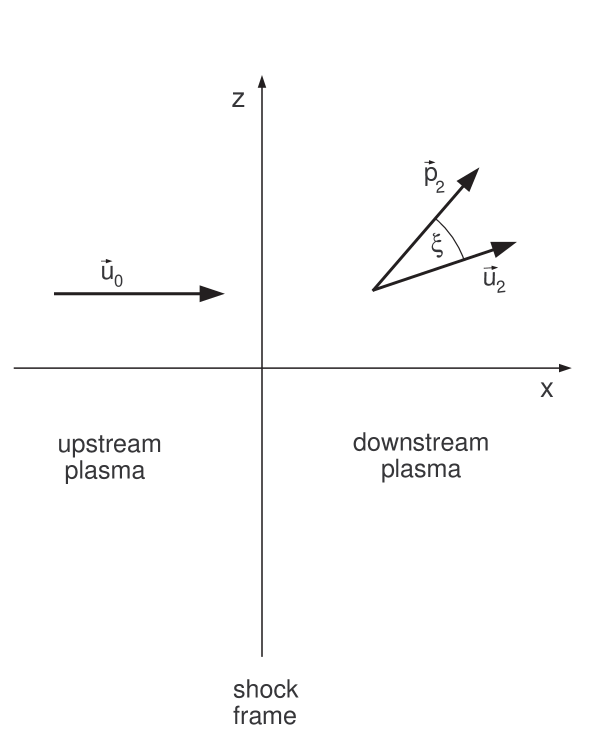
Figure 4.1: Schematic diagram showing the shock frame and a downstream particle with momentum $\vec{p_{2}}$ in the downstream frame. The downstream frame is moving with velocity $\vec{u_{2}}$ with respect to the shock frame.

Referring to Figure 4.1, the downstream plasma frame is moving with velocity $\vec{u}_{2}=\hat{x}u_{x2}+\hat{z}u_{z2}$ with respect to the shock frame, and a downstream particle has momentum $\vec{p}_{2}=\hat{x}p_{x2}+\hat{y}p_{y2}+\hat{z}p_{z2}$ in the downstream plasma frame, with the angle $\xi$ between these two vectors, where $\hat{x}$, $\hat{y}$ and $\hat{z}$ are unit vectors in the $x$, $y$ and $z$ directions. The particle momentum is defined as $\vec{p}=\gamma_{v}m\vec{v}$ where $v$ is the particle velocity, $\gamma_{v}=\left[\left(\hbox{${{\displaystyle p\vphantom{(}}\over{\displaystyle mc\vphantom{(}}}$}\right)^{2}+1\right]^{\frac{1}{2}}$ is the corresponding Lorentz factor, $p^{2}=p_{x}^{2}+p_{y}^{2}+p_{z}^{2}$, $m$ is the particle’s rest mass, and the Lorentz factor of the relative frame velocity, $\gamma_{u2}=\left(1-\hbox{${{\displaystyle u_{2}^{2}\vphantom{(}}\over{\displaystyle c^{2}\vphantom{(}}}$}\right)^{-\frac{1}{2}}$.

Before the relativistic transformations can be performed, the momentum components of the particle parallel and perpendicular to the frame velocity vector $\vec{u}_{2}$ are required. The parallel momentum component is simply the scalar product $\hat{u}\cdot\vec{p}$ where the frame velocity unit vector is $\hat{u}=\hat{x}\hbox{${{\displaystyle u_{x}\vphantom{(}}\over{\displaystyle u\vphantom{(}}}$}+\hat{z}\hbox{${{\displaystyle u_{z}\vphantom{(}}\over{\displaystyle u\vphantom{(}}}$}$, and it is understood that in these equations and the ones below where no number subscripts are used, all quantities are downstream plasma frame quantities. The momentum vector parallel to $\vec{u}$ is $\vec{p}_{\parallel}=\hat{u}(\hat{u}\cdot\vec{p})$ or

$$\vec{p}_{\parallel}=\hat{x}\left[\left(\hbox{${{\displaystyle u_{x}\vphantom{(}}\over{\displaystyle u\vphantom{(}}}$}\right)^{2}p_{x}+\left(\hbox{${{\displaystyle u_{x}u_{z}\vphantom{(}}\over{\displaystyle u^{2}\vphantom{(}}}$}\right)p_{z}\right]+\hat{z}\left[\left(\hbox{${{\displaystyle u_{x}u_{z}\vphantom{(}}\over{\displaystyle u^{2}\vphantom{(}}}$}\right)p_{x}+\left(\hbox{${{\displaystyle u_{z}\vphantom{(}}\over{\displaystyle u\vphantom{(}}}$}\right)^{2}p_{z}\right]\ .$$ (4.1)

The component of particle momentum perpendicular to the frame velocty vector is $\vec{p}_{\perp}=\vec{p}-\vec{p}_{\parallel}$ or

$$\vec{p}_{\perp}=\hat{x}\left[\left\{1-\left(\hbox{${{\displaystyle u_{x}\vphantom{(}}\over{\displaystyle u\vphantom{(}}}$}\right)^{2}\right\}p_{x}-\left(\hbox{${{\displaystyle u_{x}u_{z}\vphantom{(}}\over{\displaystyle u^{2}\vphantom{(}}}$}\right)p_{z}\right]+\hat{y}p_{y}+\hskip 71.13188pt$$

$$\hat{z}\left[\left\{1-\left(\hbox{${{\displaystyle u_{z}\vphantom{(}}\over{\displaystyle u\vphantom{(}}}$}\right)^{2}\right\}p_{z}-\left(\hbox{${{\displaystyle u_{x}u_{z}\vphantom{(}}\over{\displaystyle u^{2}\vphantom{(}}}$}\right)p_{x}\right]\ .$$ (4.2)

The relativistic momentum frame transformations from the downstream frame to the shock frame are:

$$\vec{p}_{\parallel,{sk}}=\gamma_{u}\left[\vec{p}_{\parallel}+\hbox{${{\displaystyle E\vec{u}\vphantom{(}}\over{\displaystyle c^{2}\vphantom{(}}}$}\right]=\gamma_{u}\left[\vec{p}_{\parallel}+\gamma_{v}m\vec{u}\right]$$ (4.3)

and the invariant perpendicular component of momentum

$$\vec{p}_{\perp,{sk}}=\vec{p}_{\perp}\ .$$ (4.4)

This leads to

$$\vec{p}_{sk}=\vec{p}_{\parallel,{sk}}+\vec{p}_{\perp,sk}$$ (4.5)

where

$$\vec{p}_{\parallel,{sk}}=\gamma_{u}\hat{x}\left[\left(\hbox{${{\displaystyle u_{x}\vphantom{(}}\over{\displaystyle u\vphantom{(}}}$}\right)^{2}p_{x}+\left(\hbox{${{\displaystyle u_{x}u_{z}\vphantom{(}}\over{\displaystyle u^{2}\vphantom{(}}}$}\right)p_{z}+\gamma_{v}mu_{x}\right]+\hskip 142.26378pt$$

$$\gamma_{u}\hat{z}\left[\left(\hbox{${{\displaystyle u_{x}u_{z}\vphantom{(}}\over{\displaystyle u^{2}\vphantom{(}}}$}\right)p_{x}+\left(\hbox{${{\displaystyle u_{z}\vphantom{(}}\over{\displaystyle u\vphantom{(}}}$}\right)^{2}p_{z}+\gamma_{v}mu_{z}\right]\ .$$ (4.6)

The particle momentum, now seen from the shock frame, requires the corresponding $x$, $y$ and $z$ components, where $p_{x,sk}=\hat{x}\cdot\vec{p}_{sk}$, $p_{y,sk}=\hat{y}\cdot\vec{p}_{sk}$, and $p_{z,sk}=\hat{z}\cdot\vec{p}_{sk}$. The resulting components are:

$$p_{x,{sk}}=\left[\left(\gamma_{u}-1\right)\left(\hbox{${{\displaystyle u_{x}\vphantom{(}}\over{\displaystyle u\vphantom{(}}}$}\right)^{2}+1\right]p_{x}+\gamma_{u}\gamma_{v}mu_{x}+\left(\gamma_{u}-1\right)\left(\hbox{${{\displaystyle u_{x}u_{z}\vphantom{(}}\over{\displaystyle u^{2}\vphantom{(}}}$}\right)p_{z}$$ (4.7)

and

$$p_{z,{sk}}=\left[\left(\gamma_{u}-1\right)\left(\hbox{${{\displaystyle u_{z}\vphantom{(}}\over{\displaystyle u\vphantom{(}}}$}\right)^{2}+1\right]p_{z}+\gamma_{u}\gamma_{v}mu_{z}+\left(\gamma_{u}-1\right)\left(\hbox{${{\displaystyle u_{x}u_{z}\vphantom{(}}\over{\displaystyle u^{2}\vphantom{(}}}$}\right)p_{x}\ .$$ (4.8)

The $y$ component of momentum will remain invariant under the Lorentz transformations.

Finally, the momentum components are made dimensionless by dividing through by $m_{p}u_{0}$, where $m_{p}$ is the proton rest mass and $u_{0}$ is the shock flow speed:

$$p^{\prime}_{x,sk}=\left[\left(\gamma_{u}-1\right)\left(\hbox{${{\displaystyle u_{x}\vphantom{(}}\over{\displaystyle u\vphantom{(}}}$}\right)^{2}+1\right]\left[\hbox{${{\displaystyle p_{x}\vphantom{(}}\over{\displaystyle m_{p}u_{0}\vphantom{(}}}$}\right]+\hbox{${{\displaystyle\gamma_{u}\gamma_{v}mu_{x}\vphantom{(}}\over{\displaystyle m_{p}u_{0}\vphantom{(}}}$}+\left(\gamma_{u}-1\right)\left(\hbox{${{\displaystyle u_{x}u_{z}\vphantom{(}}\over{\displaystyle u^{2}\vphantom{(}}}$}\right)\left[\hbox{${{\displaystyle p_{z}\vphantom{(}}\over{\displaystyle m_{p}u_{0}\vphantom{(}}}$}\right]$$ (4.9)

$$p^{\prime}_{y,sk}=\hbox{${{\displaystyle p_{y}\vphantom{(}}\over{\displaystyle m_{p}u_{0}\vphantom{(}}}$}$$ (4.10)

$$p^{\prime}_{z,sk}=\left[\left(\gamma_{u}-1\right)\left(\hbox{${{\displaystyle u_{z}\vphantom{(}}\over{\displaystyle u\vphantom{(}}}$}\right)^{2}+1\right]\left[\hbox{${{\displaystyle p_{z}\vphantom{(}}\over{\displaystyle m_{p}u_{0}\vphantom{(}}}$}\right]+\hbox{${{\displaystyle\gamma_{u}\gamma_{v}mu_{z}\vphantom{(}}\over{\displaystyle m_{p}u_{0}\vphantom{(}}}$}+\left(\gamma_{u}-1\right)\left(\hbox{${{\displaystyle u_{x}u_{z}\vphantom{(}}\over{\displaystyle u^{2}\vphantom{(}}}$}\right)\left[\hbox{${{\displaystyle p_{x}\vphantom{(}}\over{\displaystyle m_{p}u_{0}\vphantom{(}}}$}\right]$$ (4.11)

The relativistic transformations from the shock frame to the downstream plasma frame are generated in the same way, using the transformation

$$\vec{p}_{\parallel}=\gamma_{u}\left[\vec{p}_{\parallel_{sk}}-\gamma_{v,sk}m\vec{u}_{sk}\right]$$ (4.12)

with the final normalized equations:

$$p^{\prime}_{x,pf}=\left[\left(\gamma_{u}-1\right)\left(\hbox{${{\displaystyle u_{x}\vphantom{(}}\over{\displaystyle u\vphantom{(}}}$}\right)^{2}+1\right]p_{x,sk}-\hbox{${{\displaystyle\gamma_{u}\gamma_{v,sk}\vphantom{(}}\over{\displaystyle m\vphantom{(}}}$}u_{x}{m_{p}u_{0}}+\left(\gamma_{u}-1\right)\left(\hbox{${{\displaystyle u_{x}u_{z}\vphantom{(}}\over{\displaystyle u^{2}\vphantom{(}}}$}\right)p_{z,sk}$$ (4.13)

$$p^{\prime}_{y,pf}=\hbox{${{\displaystyle p_{y}\vphantom{(}}\over{\displaystyle m_{p}u_{0}\vphantom{(}}}$}$$ (4.14)

$$p^{\prime}_{z,pf}=\left[\left(\gamma_{u}-1\right)\left(\hbox{${{\displaystyle u_{z}\vphantom{(}}\over{\displaystyle u\vphantom{(}}}$}\right)^{2}+1\right]p_{z,sk}-\hbox{${{\displaystyle\gamma_{u}\gamma_{v,sk}mu_{z}\vphantom{(}}\over{\displaystyle m_{p}u_{0}\vphantom{(}}}$}+\left(\gamma_{u}-1\right)\left(\hbox{${{\displaystyle u_{x}u_{z}\vphantom{(}}\over{\displaystyle u^{2}\vphantom{(}}}$}\right)p_{x,sk}$$ (4.15)

where it is understood that $p^{\prime}_{x,sk}$, $p^{\prime}_{y,sk}$ and $p^{\prime}_{z,sk}$ ($p^{\prime}_{x,pf}$, $p^{\prime}_{y,pf}$ and $p^{\prime}_{z,pf}$) are momentum components in the shock frame (plasma frame) normalized by $m_{p}u_{0}$, $m$ is the mass of the particle under consideration, and $\gamma_{v,sk}$ is the Lorentz factor associated with the particle velocity as seen in the shock frame. Equations for frame transformations between the upstream plasma frame and the shock frame are generated in the same manner.

4.3 Method of calculating momentum and energy flux for parallel relativistic shocks

Ellison & Reynolds (1991) describe the Monte Carlo procedure for numerically calculating the various fluxes in the shock frame, showing the flux sums $A(x,r)$ corresponding to the number flux, $B(x,r)$ corresponding to the momentum flux, and $C(x,r)$ corresponding to the energy flux, where x refers to the x component of momentum measured in the shock frame, and $r$ is the compression ratio $u_{0}/u_{2}$.

Ellison & Reynolds (1991) also describe the general process for flux conservation across the shock, assuming no explicit particle escape. A compression ratio $r$ is chosen, the fluxes A,B, and C are calculated first for an unmodified shock, then the backpressure is used to modify the shock velocity profile through several iterations until the flux profiles converge to a stable solution. If the calculated fluxes are not constant across the shock, $r$ is varied and the process is repeated until equations (4.16, 4.17, and 4.18) are satisfied.

Recalling the flux conservation relations for parallel shocks in Chapter 3, specifically, equations (3.24) - (3.29), where $P_{xx}$ is now called $P$ and $w=e+P$, jump conditions are created across the shock. The possibility of escaping particles which carry away particle, momentum, and energy fluxes as discussed in Berezhko & Ellison (1999), is now included, to give the following equations:

$$\gamma_{0}^{2}w_{0}\frac{u_{0}^{2}}{c^{2}}+P_{0}=\gamma_{x}^{2}w_{x}\frac{u_{x}^{2}}{c^{2}}+P_{x}+F_{p}$$ (4.16)

$$\gamma_{0}^{2}w_{0}u_{0}=\gamma_{x}^{2}w_{x}u_{x}+F_{e}$$ (4.17)

The third equation results from the requirement that the number of particles is conserved across the shock [Landau & Lifshitz (1959)]:

$$\gamma_{0}n_{0}u_{0}=\gamma_{x}n_{x}u_{x}+F_{n}.$$ (4.18)

The three equations above represent the momentum density flux, the energy density flux, and the particle number density flux respectively, as viewed from the shock frame, while the number density $n$ and the enthalpy $w=e+P$ are both measured in their respective local plasma frames (Ellison & Reynolds, 1991). The terms $F_{p}$, $F_{e}$ and $F_{n}$ represent escaping momentum, energy and particle fluxes, respectively, all referenced to the shock frame. Note that the Lorentz factors are referenced to the flow velocity (as a result of the three space components of velocity). The subscript 0 refers to the far upstream frame and the subscript x refers to any frame to the right of a grid plane, as shown in Figure 1.5. Recall that the grid zones come from the original shock frame divisions along the $x$ axis within which the flow velocity is constant. Also, if both sides of equation (4.18) are multiplied by the particle rest mass , the third equation could be written as $\gamma_{0}\rho_{0}u_{0}=\gamma_{x}\rho_{x}u_{x}$.

In addition to the conservation relations, there is a relation that combines the adiabatic equation of state and the conservation of total energy, i.e. a parameterization of the ratio of specific heats appropriate to the region of interest,

$$\Gamma=1+P/(e+\rho c^{2}),$$ (4.19)

where $P$ is the kinetic pressure, $e$ is the total internal energy density including the rest mass energy, $\rho c^{2}$ is the rest mass energy density, and $\Gamma$ is the true ratio of specific heats under special conditions (Blandford & McKee, 1976). These ideas are discussed in more detail in Appendix B. Note that the compression ratio $r=u_{0}/u_{2}$ depends on $\Gamma$, making the solution to these equations nonlinear (Ellison & Reynolds, 1991).

4.4 Method for modifying the relativistic shock velocity profile

This section describes a method for modifying the shock velocity profile using the relativistic flux conservation relations, including the fluxes from escaping particles.

From equations (4.16 and 4.17), one can write

$$\gamma_{x}^{2}w_{x}\frac{u_{x}^{2}}{c^{2}}+P_{x}=B(x,r),$$ (4.20)

and

$$\gamma_{x}^{2}w_{x}u_{x}=C(x,r)$$ (4.21)

where $B(x,r)$ and $C(x,r)$ are calculated as described by Ellison & Reynolds (1991). Enthalpy $w$ can be eliminated by writing the last equation as

$$w_{x}=\frac{C(x,r)}{\gamma_{x}^{2}u_{x}}$$ (4.22)

and substituting this relation into equation (4.20). Solving for pressure $P$ we have

$$P_{x}=B(x,r)-\gamma_{x}^{2}\frac{u_{x}^{2}}{c^{2}}\frac{C(x,r)}{\gamma_{x}^{2}u_{x}}=B(x,r)-C(x,r)\frac{u_{x}(old)}{c^{2}}$$ (4.23)

where $u_{x}(old)$ is the existing velocity at grid zone position $x$.

So far, using $u_{x}(old)$, we have an estimate of the pressure. Going back to equation (4.16), it can be noted that the left hand side of this equation (far upstream from the shock) is a constant momentum flux because there are no escaping particles, so $K_{p}$ is calculated:

$$\gamma_{0}^{2}w_{0}\frac{u_{0}^{2}}{c^{2}}+P_{0}=K_{p}.$$ (4.24)

Then one can rewrite equation (4.16) as

$$K_{p}=\gamma_{x}^{2}w_{x}\frac{u_{x}^{2}}{c^{2}}+P_{x}+F_{p}$$ (4.25)

The left hand side of equation (4.17), far upstream where there are no escaping particles, yields a constant energy flux, so $K_{e}$ is calculated:

$$\gamma_{0}^{2}w_{0}u_{0}=K_{e}.$$ (4.26)

Then one can rewrite equation (4.17) as

$$K_{e}=\gamma_{x}^{2}w_{x}u_{x}+F_{e}$$ (4.27)

with

$$w_{x}=\frac{K_{e}-F_{e}}{\gamma_{x}^{2}u_{x}}.$$ (4.28)

$K_{p}$ and $K_{e}$ are numerically calculated in the same way as are $B(x,r)$ and $C(x,r)$, but far upstream and far from all velocity variations where there are no escaping particles. $F_{p}$ and $F_{e}$, the momentum and energy fluxes of escaping particles, are numerically calculated separately from $B(x,r)$ and $C(x,r)$, but in the same way as the other values.

Substituting (4.28) into (4.25), we have

$$K_{p}=(K_{e}-F_{e})\frac{u_{x}}{c^{2}}+P_{x}+F_{p}\quad,$$ (4.29)

but $u_{x}$ is an estimate of the new flow velocity:

$$u_{x}=c^{2}\frac{(K_{p}-F_{p}-P_{x})}{K_{e}-F_{e}}=u_{x}(new)\quad.$$ (4.30)

This equation can now be combined with equation (4.23) to give the new flow velocity estimate in terms of the calculated flux values:

$$u_{x}(new)=\frac{c^{2}}{(K_{e}-F_{e})}\left[K_{p}-F_{p}-B(x,r)+C(x,r)\frac{u_{x}(old)}{c^{2}}\right].$$ (4.31)

This last equation estimates the new velocity profile for the next iteration for a given compression ratio. After a number of iterations, the velocity and flux profiles should stop varying, i.e., $u_{x}(new)$ should become closer and closer to the previously calculated $u_{x}$. If, after the series of iterations, the flux profiles are constant across the shock (i.e., from upstream to downstream), then the correct compression ratio was used. If the flux profiles are not constant, the compression ratio must be varied up or down. In general, if the downstream side shows a jump upwards in momentum flux after the iterations, it means the compression ratio was too high and needs to be lowered.

4.5 Calculating $\Gamma$

After the iterations are completed and, assuming conservation of the particle, momentum and energy fluxes has been achieved, the parameter $\Gamma$ can be calculated. If the pressure and energy density are known, equation (4.19) can be used to calculate $\Gamma$ as shown in section 2.3 of Ellison & Reynolds (1991). For Lorentz factors of 10 or greater, the $\Gamma$ derived in this manner should agree very closely with the $\Gamma$ calculated from equation (3.43):

$$\Gamma=1+\beta_{2}=1+\frac{1}{r}$$ (4.32)

4.6 Summary

Relativistic momentum transformation equations were developed that relate the upstream and downstream plasma reference frames to the frame at rest with the shock. The equations allow oblique flows and arbitrary particle momentum directions.

A method was developed for modifying the relativistic shock velocity profile by using the relativistic flux conservation relations, with arbitrary magnetic field angle, to treat the momentum and energy flux at every grid zone, plus the fluxes from escaping energetic particles.

Chapter 5 The Monte Carlo Technique and Computer Simulations

The description of particle diffusion and energy gain is far more difficult when $\gamma_{0}\gg 1$ because the diffusion approximation, which requires nearly isotropic distribution functions, cannot be made. Because of this, Monte Carlo simulations, where particle scattering and transport are treated explicitly, and which, in effect, solve the Boltzmann equation with collective scattering (e.g., Ellison & Eichler, 1984; Kirk & Schneider, 1987b; Ellison, Jones, & Reynolds, 1990; Ellison & Reynolds, 1991; Ostrowski, 1991; Bednarz & Ostrowski, 1996), offer advantages over analytic methods. This is true in the test-particle approximation, where analytic results exist, but is even more important for nonlinear relativistic shocks.

In nonrelativistic shocks, for $v\gg u_{0}$, a diffusion-convection equation can be solved directly for infinite, plane shocks (e.g., Axford, Leer, & Skadron, 1977; Blandford & Ostriker, 1978), yielding the well-known result

$$f(p)\,d^{3}p\propto p^{-\sigma}\,d^{3}p\quad\hbox{with}\quad\sigma=3r/(r-1)\ ,$$ (5.1)

where $r$ is the shock compression ratio, $p$ is the momentum, and $f(p)\,d^{3}p$ is the number density of particles in $d^{3}p$. Equation (5.1) is a steady-state, test-particle result with an undetermined normalization, but the spectral index, $\sigma$, in this limit is independent of the shock speed, $u_{0}$, or any details of the scattering process as long as there is enough scattering to maintain isotropy in the local frame. To obtain an absolute injection efficiency, or to self-consistently describe the nonlinear back-reaction of accelerated particles on the shock structure (at least when the seed particles for acceleration are not fully relativistic to begin with), techniques which do not require $v\gg u_{0}$ must be used. Furthermore, for particles that do not obey $v\gg u_{0}$ additional assumptions must be made for how these particles interact with the background magnetic waves and/or turbulence, i.e., the so-called “injection problem” must be considered (see, for example, Jones & Ellison, 1991; Malkov, 1998). The Monte Carlo techniques described here make the simple assumption that all particles, regardless of energy, interact in the same way, i.e., all particles scatter elastically and isotropically in the local plasma frame with a mean free path proportional to their gyroradius. These techniques and assumptions have been used to calculate nonlinear effects in nonrelativistic collisionless shocks for a number of years with good success comparing model results to spacecraft observations (e.g., Ellison & Eichler, 1984; Ellison, Möbius, & Paschmann, 1990; Ellison, Jones, & Baring, 1999).

Early work on relativistic shocks was mostly analytical in the test particle approximation (e.g., Blandford & McKee, 1976; Peacock, 1981; Kirk & Schneider, 1987a; Heavens & Drury, 1985), although the analytical work of Schneider & Kirk (1987) explored modified shocks. Test-particle Monte Carlo techniques for relativistic shocks were developed by Kirk & Schneider (1987b) and Ellison, Jones, & Reynolds (1990) for parallel, steady-state shocks, i.e., those where the shock normal is parallel to the upstream magnetic field, and extended to include oblique magnetic fields by Ostrowski (1991). Some preliminary work on modified relativistic shocks using Monte Carlo techniques was done by Ellison (1991a, b).

Monte Carlo techniques are used to model nonlinear particle acceleration in parallel collisionless shocks of various speeds, including mildly relativistic ones. When the acceleration is efficient, the back-reaction of accelerated particles modifies the shock structure and causes the compression ratio, $r$, to increase above test-particle values. Modified shocks with small Lorentz factors can have compression ratios considerably greater than $3$ and the momentum distribution of energetic particles no longer follows a power law relation. These results may be important for the interpretation of gamma-ray bursts if mildly relativistic internal and/or afterglow shocks play an important role accelerating particles that produce the observed radiation. For $\gamma_{0}\mathrel{\hbox{\hbox to0.0pt{\hbox{\lower 4.0pt\hbox{$\sim$}}\hss}\hbox{$>$}}}10$, $r$ approaches $3$ and the so-called ‘universal’ test-particle result of $N(E)\propto E^{-2.3}$ is obtained for sufficiently energetic particles. In all cases, the absolute normalization of the particle distribution follows directly from the model assumptions and is explicitly determined.

5.1 Monte Carlo Model

The techniques used here are essentially identical to those described in Ellison, Baring, & Jones (1996) and Ellison, Jones, & Baring (1999). The differences are that the code has been made fully relativistic and only results for parallel shocks with pitch-angle diffusion are presented in this chapter. The code is steady-state, includes a uniform magnetic field, and moves particles in helical orbits, as shown in Figure 5.1. The Alfvén Mach number is assumed to be large, i.e., any effects from Alfvén wave heating in the upstream precursor are neglected. This also means the second-order acceleration of particles scattering between oppositely propagating Alfvén waves is neglected. Such an effect in relativistic plasmas with strong magnetic fields is proposed for nonlinear particle acceleration in GRBs by Pelletier (1999) (see also Pelletier & Marcowith, 1998).

The pitch angle diffusion is performed as described in (Ellison, Jones, & Reynolds, 1990) and is shown in Figure 5.1. That is, after a small increment of time, $\delta t$, a particles’ momentum vector,

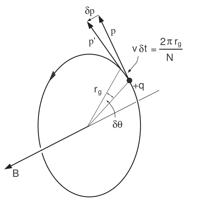
Figure 5.1: A charged particle in a helical orbit around a magnetic field vector $\vec{\mathrm{B}}$. The particle moves through an angle $\delta\theta$ in time $\delta t$. N is an input parameter chosen to contol the pitch angle granularity.

$\mathbf{p}$, undergoes a small change in direction, $\delta\theta$. If the particle originally had a pitch angle, $\theta$ (measured relative to the shock normal direction), it will have a new pitch angle $\theta^{\prime}$ such that

$$\cos{\theta^{\prime}}=\cos{\theta}\,\cos{\delta\theta}+\sqrt{1-\cos^{2}{\theta}}\sin{\delta\theta}\cos{\phi}\ ,$$ (5.2)

where $\phi$ is the azimuth angle measured with respect to the original momentum direction. All angles are measured in the local plasma frame.

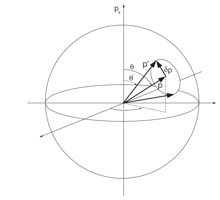
Figure 5.2: Conceptual diagram showing a particle with momentum $\vec{p}$ elastically scattering on magnetic turbulence through an angle $\delta\theta$.

If $\delta\theta$ is chosen randomly from a uniform distribution between 0 and $\delta\theta_{\mathrm{max}}$ and $\phi$ is chosen from a uniform distribution between 0 and $2\pi$, the tip of the momentum vector, referring to Figure 5.2, will perform a random walk on a sphere of radius $p$. As shown by Ellison, Jones, & Reynolds (1990), the angle $\delta\theta_{\mathrm{max}}$ is determined by

$$\delta\theta_{\mathrm{max}}=\left(6\,\delta t/t_{c}\right)^{1/2}=\left(12\pi/N\right)^{1/2}\ ,$$ (5.3)

where $N=\tau_{g}/\delta t\gg 1$ is the number of gyro-segments, $\delta t$, dividing a gyro-period $\tau_{g}=2\pi r_{g}/v$. The time $t_{c}$ is a “turn around” time defined as $t_{c}=\lambda/v$, where $\lambda$ is the particle mean free path. The mean free path is taken to be proportional to the gyroradius $r_{g}=pc/(QeB)$ ($e$ is the electronic charge, $Q$ is the ionic charge number, and $B$ is the local uniform magnetic field), i.e., $\lambda=\eta\,r_{g}$, where $\eta$ determines the strength of scattering. In all of the examples given here $\eta=1$ is set, or, in other words, the strong scattering Bohm limit is assumed.

For a downstream particle to return upstream, it’s velocity vector must be directed within a cone with opening angle $\theta_{2}$ such that $|v_{2}\cos{\theta_{2}}|>u_{2}$, where $v_{2}$ and $\theta_{2}$ are measured in the downstream frame and $\theta_{2}=0^{\circ}$ is in the $-x$-direction, i.e., along the shock normal direction. For fully relativistic shocks with $v_{2}\simeq c$ and $u_{2}\simeq c/3$, $\cos{\theta_{2}}\mathrel{\hbox{\hbox to0.0pt{\hbox{\lower 4.0pt\hbox{$\sim$}}\hss}\hbox{$>$}}}1/3$ for a downstream particle to cross the shock into the upstream region. When the particle enters the upstream region it must satisfy essentially the same constraint, i.e., $|v_{0}\cos{\theta_{0}}|>u_{0}$, where now $v_{0}$ and $\theta_{0}$ are measured in the upstream frame. Since both the particle and shock have high Lorentz factors, one can write

$$\cos{\theta_{0}}=u_{0}/v_{0}=\frac{\left(1-1/\gamma^{2}_{0}\right)^{1/2}}{\left(1-1/\gamma^{2}_{v}\right)^{1/2}}\simeq\frac{1-1/(2\gamma^{2}_{0})}{1-1/(2\gamma^{2}_{v})}\ ,$$ (5.4)

where $\gamma_{v}\equiv[1-(v_{0}/c)^{2}]^{-1/2}$ is the particle Lorentz factor. Since $\cos{\theta_{0}}\simeq 1-\theta_{0}^{2}/2$ for small $\theta_{0}$, we have

$$\theta_{0}^{2}\simeq\frac{1}{\gamma^{2}_{0}}-\frac{1}{\gamma^{2}_{v}}\ .$$ (5.5)

For ultrarelativistic particles with $\gamma_{v}\gg\gamma_{0}$, $\theta_{0}\simeq 1/\gamma_{0}$ (e.g., Gallant & Achterberg, 1999), but $\theta_{0}$ can be much smaller for mildly relativistic particles.

In order to re-cross into the downstream region, particles must scatter out of the upstream cone defined by $\theta_{0}$ and Achterberg et al. (2001) show that most particles are only able to change the angle they make with the upstream directed shock normal by $|\delta\theta|\sim\theta_{0}$ before being sweep back downstream, making the distribution of shock crossing particles highly anisotropic. Therefore, if the shock Lorentz factor $\gamma_{0}\gg 1$, a larger fraction of particles re-cross the shock into the downstream region with highly oblique angles (as measured in the shock frame) compared to lower speed shocks (see Figure 5.4 discussed below). Particles crossing at such oblique angles receive smaller energy gains than would be the case for an isotropic pitch angle distribution and Achterberg et al. (2001) go on to show that $<\!\!{E_{f}/E_{i}}\!\!>\sim 2$ for a shock crossing cycle (after the first one).

Figure 5.3: Power law spectral index, $\sigma$, versus number of gyro-segments, $N$, for various test-particle shocks as labeled. In all cases, as $N$ is increased the spectral index converges asymptotically and obtain the known results of $\sigma\simeq 4$ for nonrelativistic shocks with $r=4$, and $\sigma\simeq 4.23$ for fully relativistic shocks with $r=3$. The parameter $N_{\mathrm{min}}$ is defined in equation (5.6).

With these concepts in mind, the requirement must be $\delta\theta_{\mathrm{max}}<\theta_{0}$, or

$$N>N_{\mathrm{min}}=12\pi\gamma_{0}^{2}\ .$$ (5.6)

The result (as shown in Figure 5.3) is that the power law spectral index, $\sigma$, asymptotically approaches a maximum value as $N$ is increased. If $N$ is less than the value required for convergence to the asympotic value (and the gyro-segments are too large), the distribution will be flatter than produced with the convergent value of $N$ because more particles are able to cross from upstream to downstream with $\theta_{\mathrm{sk}}\ll 90^{\circ}$ and receive unrealistically large energy boosts. This effect has long been known from the comparison of pitch-angle diffusion to large-angle scattering in relativistic shocks (e.g., Kirk & Schneider, 1987b; Ellison, Jones, & Reynolds, 1990). For all of the examples reported on here, $N$ is chosen large enough so it makes no difference if $\delta\theta$ is chosen uniformly between $0^{\circ}$ and $\delta\theta_{\mathrm{max}}$ or if $\cos{\delta\theta}$ is chosen uniformly between $\cos{\delta\theta_{\mathrm{max}}}$ and 1. Figure 5.3 shows how the results depend on $N$ for shock speeds ranging from fully nonrelativistic to fully relativistic. In all cases, as $N$ is increased the spectral index approaches a maximum and for $\gamma_{0}\mathrel{\hbox{\hbox to0.0pt{\hbox{\lower 4.0pt\hbox{$\sim$}}\hss}\hbox{$>$}}}7$ the well known result $\sigma=4.2$–$4.3$ is obtained. The fact that the computation time for the Monte Carlo simulation scales as $N$ and $N\propto\gamma_{0}^{2}$ places limits on modeling ultrarelativistic shocks with this technique.

Figure 5.4: Distribution of the cosine of the pitch angle, i.e., $p_{x}/p_{t}$, for particles crossing $x=0$. The solid and dashed curves in the top panel are for a shock with Lorentz factor $\gamma_{0}=2$. The dotted curve in the top panel is for a nonrelativistic shock with speed $u_{0}=5000$ km s^-1. The bottom panel shows curves for a fully relativistic shock with $\gamma_{0}=10$. In all cases, the curves are normalized so that the areas under them is 1 and the $x$-component of momentum, $p_{x}$, is positive when directed downstream. The nonlinear (NL) and unmodified (UM) shock results are labeled.

In Figure 5.4 pitch-angle distributions (measured in the shock reference frame) of particles crossing the shock are compared. The curves are normalized such that the area under each curve equals one and the $x$-component of particle momentum in the shock frame, $p_{x}$, is positive when directed downstream to the right (see Figure 5.10 for the shock geometry). Here, $p_{t}$ is the magnitude of the total particle momentum also measured in the shock frame. In the top panel, unmodified (UM) test particle and nonlinear (NL) mildly relativistic shock ($\gamma_{0}=2$) with a nonrelativistic one ($u_{0}=5000$ km s^-1) are compared. Particles crossing the $\gamma_{0}=2$ shock are highly anisotropic with $p_{x}/p_{t}$ strongly peaked near $\sim 0.35$. In the nonrelativistic shock, the particles are nearly isotropic except for a slight flux-weighting effect. There is little difference in the distributions between the UM and NL shocks. In the bottom panel, the pitch-angle distributions for UM and NL shocks with $\gamma_{0}=10$ are shown. While the distributions are somewhat more sharply peaked, they are quite similar to those for $\gamma_{0}=2$ and show relatively small variations between the UM and NL shocks.

The main difference between the present code and an earlier code used by Ellison, Jones, & Reynolds (1990) to model test-particle relativistic shocks is that the previous code used a guiding center approximation with an emphasis on large-angle scattering rather than the more explicit orbit calculation of pitch-angle diffusion used here. Other than the far greater range in $\gamma_{0}$ and the nonlinear results presented here, the work of Ellison, Jones, & Reynolds (1990) is consistent with this work.

The particle transport is performed as follows. Particles of some momentum, $p_{\mathrm{pf}}$, (measured in the local plasma frame) are injected far upstream from the shock and pitch-angle diffuse and convect until they cross a grid zone boundary, i.e., a plane with its normal parallel to the upstream flow speed (see Ellison, Baring, & Jones, 1996, for a full discussion). For unmodified shocks, the flow speed changes from the upstream to downstream value in a discontinuous step at the shock boundary, but for nonlinear shocks the bulk flow speed changes in small steps, each separated by a grid zone boundary, from $u_{0}$ far upstream to $u_{2}$ downstream. In the unmodified case, the shock thickness is essentially zero (i.e., shorter than the distance a particle diffuses in $\delta t$) but in the nonlinear, modified case, the shock precursor extends over the entire region of varying bulk flow speeds and a small scale “subshock” (at position $x=0$ in this simulation) exists where most of the entropy production occurs. When a particle crosses a grid zone boundary, $p_{\mathrm{pf}}$ is transformed to the new local frame moving with a new speed relative to the subshock and the particle continues to scatter and convect. Each particle is followed until it leaves the system in one of three ways. It can convect far downstream and not return to the subshock, it can obtain a momentum greater than some $p_{\mathrm{max}}$ and be removed, or it can diffuse far enough upstream to cross an upstream free escape boundary (FEB) and be removed. Both $p_{\mathrm{max}}$ and the position of the FEB are free parameters in this model (see Berezhko & Völk, 1997, for a discussion of the self-consistent determination of the maximum particle energy in nonrelativistic supernova remnant shocks). For the nonlinear calculations, the shock structure and compression ratio are iterated until the number, momentum, and energy fluxes are conserved across the shock. This procedure has been detailed many times for nonrelativistic shocks (see Ellison, Baring, & Jones, 1996, and references therein) and the modifications required for relativistic shocks were given in Ellison & Reynolds (1991).

To avoid excessive computation, a probability of return calculation as described in detail in Ellison, Jones, & Reynolds (1990) is used. That is, the standard expression obtained by Peacock (1981) is used,

$$P_{R}=\left(\frac{v-u_{2}}{v+u_{2}}\right)^{2}\ ,$$ (5.7)

to determine the probability, $P_{R}$, that a particle, having crossed a particular point in the uniform downstream flow, will return back across that point. Equation (5.7) is fully relativistic and independent of the diffusive properties of the particles as long as they are isotropic in the $u_{2}$ frame. This isotropy is ensured by only applying equation (5.7) once a particle has diffused several mean free paths downstream from the shock. For ultrarelativistic shocks with $v\simeq u_{0}\simeq c$ and $r\simeq 3$, equation (5.7) gives $P_{R}\simeq 0.25$.

For clarity, it is noted that this is not the same probability, ${\cal P_{\mathrm{ret}}}$, used by Achterberg et al. (2001) to determine the test-particle power law index, i.e.,

$$s=1+\frac{\ln(1/{\cal P_{\mathrm{ret}}})}{\ln<\!\!{E_{f}/E_{i}}\!\!>}\ ,$$ (5.8)

where $N(E)\propto E^{-s}$ and, for fully relativistic particles, $s=\sigma-2$. The quantity $<\!\!{E_{f}/E_{i}}\!\!>$ is the average energy ratio for a particle undergoing a shock crossing cycle. Although not explicitly stated in Achterberg et al. (2001), it is clear from the context that ${\cal P_{\mathrm{ret}}}$ is calculated just behind the shock where the particle distribution is highly anisotropic. In this case, particles that have just crossed from upstream to downstream will be more likely to recross back into the upstream region than indicated by equation (5.7) because their pitch angles are more likely to be highly oblique relative to the shock normal than in the isotropic distributions further downstream (compare the solid or dashed curves to the dotted curve in the top panel of Figure 5.4 discussed below). For $\gamma_{0}=10$, Achterberg et al. (2001) find ${\cal P_{\mathrm{ret}}}=0.435\pm 0.005$ and $<\!\!{E_{f}/E_{i}}\!\!>=1.97\pm 0.01$ giving the standard result $s=2.230\pm 0.012$. As shown in Figure 5.3, the unmodified results are consistent with this spectral index for $\gamma_{0}\mathrel{\hbox{\hbox to0.0pt{\hbox{\lower 4.0pt\hbox{$\sim$}}\hss}\hbox{$>$}}}7$.

Figure 5.5: Particle spectra, $p^{4}f(p)$, versus momentum for various unmodified shocks with speeds as indicated. The test-particle compression ratios, $r$, and spectral indices, $\sigma$, are noted. The far upstream plasmas in the 5000 km s^-1, and $\beta_{0}=0.5$ shocks are thermal at $10^{6}$ K. The $\gamma_{0}=10$ shock has a far upstream plasma which is a $\delta$-function at 1 MeV. All spectra are calculated at the shock, in the shock frame, and the relative normalization is arbitrary.

5.2 Test-Particle Results

In Figure 5.5 particle distributions for unmodified shocks are shown with speeds ranging from fully nonrelativistic ($u_{0}=5000$ km s^-1) to mildly relativistic ($\beta_{0}=u_{0}/c=0.5$) to fully relativistic ($\gamma_{0}=10$). The nonrelativistic distribution matches the standard test-particle Fermi result of $\sigma=4$ for $r=4$ and the fully relativistic result is consistent with the well-known limit of $\sigma\,\rightarrow\,4.2-4.3$ as $\gamma_{0}\,\rightarrow\,\infty$ for $r=3$. In the trans-relativistic regime, both the compression ratio and the spectral index vary with $u_{0}$. For the $u_{0}=0.5c$ distribution shown in Figure 5.5, the compression ratio was determined by balancing the mass, momentum, and energy fluxes across the shock in the test-particle limit, i.e., by ignoring any effects from the accelerated particles. This technique is described in detail in Ellison & Reynolds (1991). It was found that $r=3.8\pm 0.1$ and the spectral index is $\sigma\simeq 4.01$, slightly flatter than $3\,r/(r-1)\simeq 4.07$, the nonrelativistic result.

Figure 5.6: The solid line is the compression ratio, $r$, and the dashed line is the spectral index, $\sigma$, for unmodified (i.e., test-particle) shocks. The solid dots show $r$ for shocks undergoing efficient particle acceleration. In all cases, $r$ is determined for each $\beta_{0}\gamma_{0}$ by balancing the momentum and energy fluxes across the shock. The maximum cutoff momentum, $p_{\mathrm{max}}$, is unimportant for the test-particle shocks, but is set to $10^{4}\,\beta_{0}\gamma_{0}\,m_{p}c$ for the nonlinear shocks.

Figure 5.6 shows the compression ratio as a function of $\beta_{0}\gamma_{0}$ (solid curve), still ignoring the effects of accelerated particles. The compression ratio is determined self-consistently by balancing the momentum and energy fluxes across the shock with no restriction on the shocked or unshocked adiabatic index. As expected, $r$ decreases smoothly from $4$ for fully nonrelativistic shocks to $\sim 3$ for fully relativistic shocks. The power law index, $\sigma$, is also shown (dashed curve) and this varies slowly from $\sigma=4$ to $\sigma\simeq 4.23$ between the two extremes. For comparison, $r$ (solid dots) is shown for shocks undergoing efficient particle acceleration. For these points, all shock parameters except $\beta_{0}\gamma_{0}$ and $p_{\mathrm{max}}$ are kept constant. For the nonlinear shocks, the maximum cutoff momentum is set to $p_{\mathrm{max}}=10^{4}\,\beta_{0}\gamma_{0}\,m_{p}c$ in all cases. The nonlinear results are discussed in detail below, but here only emphasize that $r$ in nonlinear shocks will be larger than the test-particle value for $\gamma_{0}\mathrel{\hbox{\hbox to0.0pt{\hbox{\lower 4.0pt\hbox{$\sim$}}\hss}\hbox{$<$}}}10$. The test-particle results shown in Figure 5.6 are in close agreement with recent analytic results of Kirk et al. (2000) and Gallant (2002). It seems that no analytic results exist for nonlinear, relativistic shocks.

Figure 5.7: Average ratios of final (f) to initial (i) momentum for downstream to upstream to downstream and upstream to downstream to upstream shock crossing cycles. The histograms are for a test-particle shock with $\gamma_{0}=10$ and $r=3$. Note the large momentum gain ($<\!\!{p_{f}/p_{i}}\!\!>_{\mathrm{u-d-u}}=115$) in the first shock crossing cycle. Note also that this particular value depends on the choice of the injection momentum.

In Figure 5.7 the average ratios of momenta are shown (measured in the local plasma frame) for particles executing upstream to downstream to upstream cycles across the shock, $<\!\!{p_{f}/p_{i}}\!\!>_{\mathrm{u-d-u}}$, and downstream to upstream to downstream cycles, $<\!\!{p_{f}/p_{i}}\!\!>_{\mathrm{d-u-d}}$. These results are for $\gamma_{0}=10$ ($r=3$) and show a slight momentum dependence at low momenta but converge to $<\!\!{p_{f}/p_{i}}\!\!>=2.2\pm 0.1$ at high momenta. This value is close to $<\!\!{E_{f}/E_{i}}\!\!>=1.97\pm 0.01$ reported by Achterberg et al. (2001) for $\gamma_{0}=10$. As mentioned above, in the first upstream to downstream to upstream cycle, particles achieve a large boost in momentum as indicated in the figure.

The difference between this value of $<\!\!{p_{f}/p_{i}}\!\!>$ at large $p_{i}$ and that of Achterberg et al. (2001) is greater than the uncertainties and probably stems from the different assumptions made in the simulations. As discussed above, $<\!\!{p_{f}/p_{i}}\!\!>$ depends critically on the average angle a particle makes when crossing the shock. While the large majority of particles in these simulations gain energy by crossing from downstream to upstream and then immediately (within a few $\delta t$’s) re-crossing back into the downstream region at oblique angles, a few manage to diffuse farther upstream (see Figure 5.9 below). When these particles re-cross the shock into the downstream region, they can do so at flatter angles and receive larger energy gains. One might speculate that differences in how these few particles are treated in the simulations might produce the differences in $<\!\!{p_{f}/p_{i}}\!\!>$.

As an illustration of how particles interact with nonrelativistic and relativistic unmodified shocks, trajectories for two individual particles are shown in Figures 5.8 and 5.9. The lower panel in each figure shows a trace of the particle trajectory and the upper panels show the particle momentum, always measured in the local plasma frame. For the nonrelativistic shock (Figure 5.8), the speed of the particle is far greater than the shock speed and it diffuses easily on both sides of the shock. When it crosses $x=0$, it does so nearly isotropically (except flux weighting makes crossings with flat trajectories slightly more likely) and essentially always gains momentum. The momentum gain in a single shock crossing is small, but a particle can stay in the system for many crossings.

When the shock speed, $u_{0}$, is close to $c$, the particle will be convected downstream much more rapidly than in nonrelativistic shocks and few particles will be able to cross the shock many times. However, downstream particles that do manage to cross the shock into the upstream region do so with much flatter trajectories, as discussed above, and can receive large momentum boosts in a single shock crossing due to the shock’s Lorentz factor (note the logarithmic scale in the top panel of Figure 5.9). In a typical shock crossing cycle, downstream particles gain momentum when they cross into the upstream region (see positions labeled $a$ and $b$ in Figure 5.9), lose momentum when they cross back downstream because they cross with oblique pitch angles, but end up with a net momentum boost. However, as shown by the position labeled $c$, it is possible for a particle to diffuse farther upstream before being convected back to the shock. In this case, it can cross the shock with a flat trajectory and gain momentum upon entering the downstream region. If the acceleration is efficient, the few particles that diffuse far upstream carry enough pressure to produce the shock smoothing discussed next.

Figure 5.8: Particle trajectory (lower panel) and momentum (upper panel) in an unmodified shock of speed $u_{0}=5000$ km s^-1. The momentum is calculated in the local plasma frame, either upstream or downstream from the shock.

Figure 5.9: Trajectory and momentum for a particle in an unmodified shock with speed $u_{0}=0.9c$. Note that the horizontal axis is split at 1200 scatterings. Note also that the momentum scale is logarithmic because the momentum excursions are very large.

5.3 Non-Linear Results

As noted by Achterberg et al. (2001), the large energy boost particles receive in their initial crossing of the shock provides a natural injection process for further acceleration and suggests that relativistic shocks may be efficient accelerators. However, just as with nonrelativistic shocks, efficient acceleration limits the use of test-particle approximations and requires that the nonlinear back-reaction of the accelerated particles be treated self-consistently (e.g., Jones & Ellison, 1991). These nonlinear effects will result in a smoothing of the shock and a change in the overall shock compression ratio, just as they do in nonrelativistic shocks. The differences between test-particle and nonlinear results, for the parameter ranges investigated here, are large enough to produce spectra noticeably different from the often quoted $N(E)\propto E^{-2.3}$ and to influence applications to GRB models where high shock efficiencies are assumed. This is illustrated with two examples, one mildly relativistic ($\gamma_{0}=1.4$) and one more fully relativistic ($\gamma_{0}=10$). The far upstream conditions have relatively little influence on the results as long as $\gamma_{p}\ll\gamma_{0}$, where $\gamma_{p}$ is the plasma frame Lorentz factor of the far upstream, injected particles. For concreteness, in both examples the far upstream plasma is taken to be a thermal distribution of leptons and baryons at a temperature of $10^{6}$ K, but only baryon acceleration is considered; the electrons only being included for charge neutrality.

5.3.1 Mildly relativistic shock: $\gamma_{0}=1.4$

Figure 5.10: Unmodified (UM) and nonlinear (NL) shock profiles, i.e., $\gamma_{u}(x)u(x)$, and momentum and energy fluxes versus position, $x$. All quantities are scaled to far upstream values and in all panels the solid curves are results from unmodified shocks and the dashed curves are nonlinear results. The NL momentum and energy fluxes are 3 to 4% below the far upstream values because particles escape at a maximum momentum, $p_{\mathrm{max}}=10^{4}\beta_{0}\gamma_{0}m_{p}c\simeq 10^{13}$ eV/c. $N/N_{\mathrm{min}}\sim 10$ have been used in both cases.

Figure 5.10 shows unmodified and nonlinear shock structures for $\gamma_{0}=1.4$. The top panel shows $\gamma_{u}(x)\,u(x)$, where $\gamma_{u}(x)=\{1-[u(x)/c]^{2}\}^{-1/2}$, the middle panel is momentum flux, and the bottom panel is the energy flux, all scaled to far upstream values. All curves are plotted versus $x$, where $x=0$ is the position of the sharp subshock. A logarithmic scale is used for $x<-10\,r_{g,0}$ and a linear scale is used for $x>-10\,r_{g,0}$, where $r_{g,0}\equiv m_{p}u_{0}/(eB)$. In each panel, the solid curve is from an unmodified shock with $r\simeq 3.6$ (see Figure 5.6), while the dashed curve is the momentum and energy flux conserving result.

For the pitch angle diffusion model, where particles interact elastically and isotropically in the local frame according to equation (5.2) and the discussion following it, particles are accelerated efficiently enough at the unmodified shock that the momentum and energy fluxes are not conserved and rise well above the allowed far upstream values. In order to conserve these fluxes, the shock structure must be smoothed and the overall compression ratio increased above the test-particle value. The computational scheme calculates this compression ratio and flux conserving profile and the result is the dashed curve in the top panel with the corresponding momentum and energy fluxes in the middle and bottom panels.

The source of the non-conservation of momentum and energy is the efficient acceleration of particles by the sharp flow speed discontinuity. While the actual injection and acceleration efficiency depends on the particular pitch angle diffusion model, once the scattering assumptions are made, the kinematics determine the injection and acceleration of the particles without additional parameters. Of course it would have been possible to make assumptions which resulted in an acceleration efficiency low enough that momentum and energy are approximately conserved without significantly smoothing the shock structure or changing the compression ratio from the test-particle value. For example, one could have only allowed shocked particles above some Lorentz factor $\gamma_{\mathrm{inj}}$ to recross into the upstream region or arbitrarily restricted the number of particles that recrossed into the upstream to a small fraction, $f_{\mathrm{inj}}$, of all downstream particles. By making $f_{\mathrm{inj}}$ low enough or $\gamma_{\mathrm{inj}}$ high enough one could make the efficiency as low as desired. However, there are at least three reasons for not making such an assumption. The first is that restricting the acceleration efficiency requires additional parameters (i.e., $\gamma_{\mathrm{inj}}$ and/or $f_{\mathrm{inj}}$) to those needed to describe pitch angle diffusion. The second is that models with inefficient acceleration will not help explain GRBs (or other objects) that require high efficiencies. If relativistic shocks are inefficient accelerators they are not very interesting. If they are efficient, they will have a qualitative resemblance to the results shown here even if, as is likely, the actual plasma processes are far more complex than the simple model we use. A third, perhaps less compelling, reason is that identical scattering assumptions as used here have been used for some time in nonrelativistic shocks and shown to match both spacecraft observations (e.g., Ellison, Möbius, & Paschmann, 1990) and hybrid plasma simulations (e.g., Ellison et al., 1993) of collisionless shocks.

The increase in compression ratio from $r\simeq 3.6$ to $\simeq 4.5$ shown in Figure 5.10 comes about, in part, because the particles escaping at $p_{\mathrm{max}}$ carry away momentum and energy fluxes which make the shocked plasma more compressible. This effect is countered to some degree by the fact that the self-consistent shock produces a downstream distribution with a smaller fraction of relativistic particles than the test-particle shock so that the downstream ratio of specific heats $\Gamma>4/3$. This tends to produce a smaller compression ratio. The escaping fluxes show up as a lowering of the dashed curves below the far upstream values, as shown in the bottom two panels of Figure 5.10, and amount to about 3% of the far upstream values for both momentum and energy. Including the escaping fluxes, the momentum and energy fluxes are conserved to within a few percent of the far upstream values. While the changes seen here are similar to those seen and discussed for many years in efficient, nonrelativistic shock acceleration (see Berezhko & Ellison, 1999, and references therein), it must be noted that there are no known analytic expressions relating escaping fluxes and $\Gamma$ to $r$ in this trans-relativistic regime. One obvious difference is that for nonrelativistic shocks, the escaping momentum flux is generally much less than the escaping energy flux (when both are measured as fractions of incoming flux) since $\rho_{e}v_{e}^{3}/(\rho_{0}u_{0}^{3})\gg\rho_{e}v_{e}^{2}/(\rho_{0}u_{0}^{2})$ when $v_{e}\gg u_{0}$ (see Ellison, 1985). Here, $v_{e}$ is the velocity of the escaping particle. In relativistic shocks, $v_{e}\sim u_{0}\sim c$ so the escaping fluxes are about equal as shown in Figure 5.10.

Figure 5.11: Particle distributions, $p^{4}f(p)$, for the shocks shown in Figure 5.10. The nonlinear spectrum (dashed curve) shows the distinctive concave shape seen in efficient nonrelativistic shock acceleration, and has a greater fraction of low momentum particles than the spectrum from the unmodified shock. As in Figure 5.5, the spectra are calculated at the shock in the shock frame and truncated with a $p_{\mathrm{max}}$. Unlike Figure 5.5, the normalization here shows the actual acceleration efficiency.

In Figure 5.11 $p^{4}f(p)$ is plotted for the $\gamma_{0}=1.4$ shock. The solid curve is from an unmodified (UM) shock and the dashed curve is the nonlinear (NL) result. The shock smoothing and increase in $r$ produce substantial differences in the spectra even though both shocks have exactly the same input conditions. (i) The overall normalization of the NL spectrum is less, reflecting the conservation of energy flux. (ii) The NL result has the distinctive concave curvature seen in nonrelativistic shocks stemming from the fact that higher momentum particles have a longer upstream diffusion length and get accelerated more efficiently than lower momentum particles in the smooth shock. (iii) The slope at the highest momentum in the NL spectrum reflects the overall compression ratio and is flatter than the TP spectrum because $r$ is greater. (iv) The “thermal” peak is shifted to lower momentum in the NL result and contains a larger fraction of mildly relativistic particles than in the UM result, i.e., $\Gamma\simeq 1.41$ for the NL shock compared to $\Gamma\simeq 1.36$ for the UM shock.

5.3.2 Fully relativistic, nonlinear shock: $\gamma_{0}=10$

Figure 5.12: Unmodified (UM: solid curves) and nonlinear (NL: dashed curves) shock profiles as in Figure 5.10 for $\gamma_{0}=10$. The acceleration is truncated by $p_{\mathrm{max}}=10^{4}\beta_{0}\gamma_{0}m_{p}c$ and $N/N_{\mathrm{min}}\sim 10$ in both cases.

Figure 5.12 shows results for $\gamma_{0}=10$. In all panels, the solid curves are for the unmodified shock, while the dashed curves are for the flux conserving smoothed shock, both with identical input parameters. As before, the acceleration is truncated with a $p_{\mathrm{max}}=10^{4}\beta_{0}\gamma_{0}m_{p}c\simeq 9.3\!\times\!10^{13}$ eV/c. In Figure 5.13, $u(x)$ and $\gamma_{u}(x)$ are plotted separately. Even though the length-scale of the shock smoothing is only a few $r_{g,0}$ and the change in $r=3.03\pm 0.01$ is small, they bring the momentum and energy fluxes into balance from values a factor of five too large in the unmodified shock. The less than 1% difference between $r=3.03\pm 0.01$ and the canonical value of 3 is significant; a self-consistent solution does not exist outside of this range.

Figure 5.13: The top panel is the flow speed at $x$ normalized to the far upstream shock speed, $u_{0}$ versus $x$, for the $\gamma_{0}=10$ shocks shown in Figure 5.12. The bottom panel is the flow Lorentz factor, $\gamma_{u}(x)$, versus $x$. In both panels, the solid curves are the unmodified shock results with $r=3$ and the dashed curves are the nonlinear results with $r\simeq 3.03\pm 0.01$.

As discussed above, both the shock structure and the overall compression ratio may be modified when particle acceleration is efficient. For mildly relativistic shocks, such as the $\gamma_{0}=1.4$ example, a unique solution can be determined directly from the conserved momentum and energy fluxes. For larger $\gamma_{0}$’s however, the fluxes are less sensitive to changes in the structure and compression ratio and an additional constraint is needed to obtain a unique solution. This constraint is provided by the relativistic jump conditions for momentum and energy, i.e.,

$$\gamma_{u0}^{2}w_{0}\frac{u_{0}^{2}}{c^{2}}+P_{0}=\gamma_{u2}^{2}w_{2}\frac{u_{2}^{2}}{c^{2}}+P_{2}\ ;$$ (5.9)

$$\gamma_{u0}^{2}w_{0}u_{0}=\gamma_{u2}^{2}w_{2}u_{2}\ ,$$ (5.10)

where $w=e+P$ is the enthalpy density, $e$ is the total energy density, $P$ is the pressure, and it is assumed that escaping fluxes are negligible. The energy density and pressure are related through a combination of the adiabatic equation of state and the conservation of energy, i.e.,

$$P=(\Gamma-1)(e-\rho c^{2})\ ,$$ (5.11)

where $\rho c^{2}$ is the rest mass energy density and $\Gamma$ is, in special cases, the ratio of specific heats (e.g., Ellison & Reynolds, 1991). Dividing equation (5.9) by equation (5.10) yields

$$\frac{u_{0}}{c^{2}}+\frac{P_{0}}{\gamma_{u0}^{2}(e_{0}+P_{0})u_{0}}=\frac{u_{2}}{c^{2}}+\frac{P_{2}}{\gamma_{u2}^{2}(e_{2}+P_{2})u_{2}}\ ,$$ (5.12)

or, in terms of beta’s,

$$\beta_{0}+\left(\frac{P_{0}}{e_{0}+P_{0}}\right)\frac{1-\beta_{0}^{2}}{\beta_{0}}=\beta_{2}+\left(\frac{P_{2}}{e_{2}+P_{2}}\right)\frac{1-\beta_{2}^{2}}{\beta_{2}}\ .$$ (5.13)

The second term on the left hand side is small compared to $\beta_{0}$ for unshocked upstream particle temperatures less than $10^{9}$K and upstream particle densities less than $100$ cm^-3. Neglecting this term, equation (5.13) becomes

$$\beta_{0}=\beta_{2}+\left(\frac{P_{2}}{e_{2}+P_{2}}\right)\frac{1-\beta_{2}^{2}}{\beta_{2}}\ ,$$ (5.14)

or,

$$e_{2}\beta_{2}^{2}-\beta_{0}(e_{2}+P_{2})\beta_{2}+P_{2}=0\ ,$$ (5.15)

which has the shock solution

$$\beta_{2}=\beta_{0}/r=\frac{1}{2e_{2}}\left[\beta_{0}(e_{2}+P_{2})-\sqrt{\beta_{0}^{2}(e_{2}+P_{2})-4e_{2}P_{2}}\right]\ .$$ (5.16)

For $\gamma_{0}\mathrel{\hbox{\hbox to0.0pt{\hbox{\lower 4.0pt\hbox{$\sim$}}\hss}\hbox{$>$}}}10$, $\beta_{0}\simeq 1$ and $r\simeq e_{2}/P_{2}$. Furthermore, if ultrarelativistic downstream particle speeds can be assumed so that $e_{2}\gg\rho_{2}c^{2}$, equation (5.16) reduces to,

$$r\simeq\frac{1}{\Gamma_{2}-1}\ .$$ (5.17)

For $\Gamma_{2}=4/3$, $r\simeq 3$, the standard ultrarelativistic result.

Figure 5.14: Particle distributions, $p^{4}f(p)$, for the shocks shown in Figures 5.12 and 5.13 with $\gamma_{0}=10$. The spectra for the nonlinear (NL) and unmodified (UM) shocks are labeled and both are calculated at $x=0$ in the shock frame. The light-weight solid lines show spectral indexes, $\sigma=4.23$.

To obtain a unique shock solution for $\gamma_{0}\mathrel{\hbox{\hbox to0.0pt{\hbox{\lower 4.0pt\hbox{$\sim$}}\hss}\hbox{$>$}}}3$, both the shock structure and the compression ratio, $r_{\mathrm{MC}}$, are modified for the Monte Carlo simulation, $P_{2}$ and $e_{2}$ are calculated from the resultant downstream particle distributions, and $r_{\mathrm{MC}}\simeq r$ as determined from equation (5.16) are checked. If $r_{\mathrm{MC}}\neq r$, the shock structure and $r_{\mathrm{MC}}$ are varied until a consistent solution is found. For smaller $\gamma_{0}$’s, equation (5.16) doesn’t apply because escaping fluxes become significant. In this case, however, the changes in the momentum and energy fluxes from changes in the shock structure and $r_{\mathrm{MC}}$ are large enough that a unique solution can be found easily, as in the $\gamma_{0}=1.4$ example.

Despite the fact that $u(x)$ is modified on a fairly small length scale, the resultant particle distribution function is changed substantially, as indicated in Figure 5.14. In this figure, the solid curve is from the unmodified shock and the dashed curve is from the nonlinear shock, both having exactly the same input conditions. The unmodified spectrum in Figure 5.14 is similar to that shown with a dashed curve in Figure 5.5 only now the far upstream plasma is taken to be a thermal gas at a temperature of $10^{6}$ K rather than a delta function distribution of particles with speeds, $v_{\mathrm{inj}}=(2E_{\mathrm{inj}}/m_{p})^{1/2}$, with $E_{\mathrm{inj}}=1$ MeV, as was assumed for the example in Figure 5.5.

The shock smoothing has caused the low energy portion of the distribution to steepen and the overall intensity to decrease, reflecting the fact that the NL spectrum conserves momentum and energy while the UM one doesn’t. The peaks in the two distributions at low momenta are also very different, with the NL spectrum having a larger fraction of slower particles than the UM one. These peaks result from the first shock crossing where all particles receive a large energy gain. In the UM case, a far greater fraction of the accelerated downstream particles are able to receive further energization by recrossing back into the upstream region than in the NL shock. The different speed distributions result in different $\Gamma$’s and it was found, by directly calculating $\Gamma$ from the distributions, that $\Gamma_{\mathrm{UM}}\simeq 1.34$ while $\Gamma_{\mathrm{NL}}\simeq 1.36$.

5.3.3 Acceleration efficiency

Figure 5.15: Acceleration efficiency, $\epsilon(>p)$, defined as the fraction of total kinetic energy density above $p$ versus $p$, is shown for two nonlinear cases. The sharp dropoff at low momenta indicates the extent of the ‘thermal’ peak.

The absolute acceleration efficiency can be determined in the self-consistent, nonlinear examples directly from the particle distributions. In Figure 5.15, $\epsilon(>p)$ is plotted, i.e., the fraction of kinetic energy density above a momentum $p$ versus $p$ for the $\gamma_{0}=1.4$ and $\gamma_{0}=10$ examples. The fraction of kinetic energy in the quasi-thermal part of the distribution can be determined from the relatively sharp fall off of the distributions at low momenta. This occurs near $m_{p}c$ for $\gamma_{0}=1.4$ and near $10\,m_{p}c$ for $\gamma_{0}=10$. If the acceleration efficiency is somewhat arbitrarily defined for these two examples to be $\epsilon_{1.4}(>m_{p}c)$ and $\epsilon_{10}(>10m_{p}c)$, respectively, the result is $\epsilon_{1.4}(>m_{p}c)\simeq 0.7$ and $\epsilon_{10}(>10m_{p}c)\simeq 0.6$. Of course, the behavior of $\epsilon(>p)$ depends on the particle spectrum from which it is derived and thus $\epsilon(>p)$ is flatter for the $\gamma_{0}=1.4$ shock, with $r\simeq 4.5$, than for the $\gamma_{0}=10$ shock, where $r\simeq 3.03\pm 0.01$. Furthermore, $\epsilon(>p)$ depends strongly on $p_{\mathrm{max}}$ in the $\gamma_{0}=1.4$ shock where particle escape plays an important role in determining $r$. The maximum momentum has little influence for $\gamma=10$ because of the steep spectrum. The fraction of kinetic energy density above $10^{3}m_{p}c$ is about 0.3 for $\gamma_{0}=1.4$ and about 0.1 for $\gamma_{0}=10$.

5.4 Summary

Particles gain energy in collisionless shocks by scattering nearly elastically off magnetic turbulence, back and forth between the converging plasmas upstream and downstream from the shock. While this basic shock acceleration physics is independent of the speed of the shock, the mathematical modeling of the process depends critically on whether or not the acceleration is efficient and whether or not particle speeds, $v$, are large compared to the shock speed, $u_{0}$. The Monte Carlo techniques discussed here, which do not require $v\gg u_{0}$, are well suited for the study of relativistic shocks, and for any shock where nonlinear effects are important and the energetic particles originate as thermal particles in the unshocked plasma. Except for computational limits, these techniques allow calculations of efficient particle acceleration in shocks of any Lorentz factor.

As a check of the Monte Carlo code, it was demonstrated that the well known test-particle power laws can be obtained in fully nonrelativistic and ultrarelativistic shocks (Figures 5.3 and 5.5). In trans-relativistic shocks, however, no such canonical results exist because the shock compression ratio, $r$, depends on the upstream conditions in a nonlinear fashion, even for test-particle shocks where all effects of accelerated particles are ignored (e.g., Ellison & Reynolds, 1991). it was shown how $r$, and the resulting power law spectral index, $\sigma$, vary through the trans-relativistic regime in Figure 5.6, where $r$ has been determined by balancing the momentum and energy fluxes across the shock in an iterative process. These test-particle results with self-consistently determined compression ratios are in close agreement with the recent analytic results of Kirk et al. (2000) and Gallant (2002).

Despite the fact that relativistic shock theory has concentrated almost exclusively on test-particle acceleration, it is likely that relativistic shocks are not test-particle but inject and accelerate particles efficiently. The reason is that regardless of the ambient far upstream conditions, particles that are overtaken by an ultrarelativistic shock will receive a large boost in energy $\sim\gamma_{\mathrm{rel}}$ in their first shock crossing. Thus, virtually all of the particles in the downstream region of an unmodified shock are strongly relativistic with $v\sim c$ as seen in the downstream frame. The ability to overtake the shock from downstream and be further accelerated depends only on the particle speed (equation 5.7) and the presence of magnetic waves or turbulence with sufficient power in wavelengths on the order of the particle gyroradii to isotropize the downstream distributions. It is generally assumed that the necessary magnetic turbulence is self-generated and if enough turbulence is generated to scatter high momentum particles (with very low densities) that constitute a test-particle power law, there should be enough generated to isotropize lower momentum particles (which carry the bulk of the density). If acceleration can occur at all, it is believed that it is likely to occur efficiently making it necessary to calculate the shock structure and particle acceleration self-consistently. Furthermore, if relativistic shock theory is to be applied to gamma-ray bursts, where high conversion efficiencies are generally assumed, nonlinear effects must be calculated.

When energetic particles are generated in sufficient numbers, the conservation of momentum and energy requires that their backpressure modify the shock structure. Two basic effects occur: a precursor is formed when the upstream plasma is slowed by the backpressure of the accelerated particles and the overall compression ratio changes from the test-particle value as a result of high energy particles escaping and/or a change in the shocked plasma’s ratio of specific heats, $\Gamma$. As indicated by the $\gamma_{0}=1.4$ example (Section 5.3.1), mildly relativistic shocks act as nonrelativistic shocks, showing a dramatic weakening of the subshock combined with a large increase in $r$ (Figure 5.10). These changes result in a particle distribution which is both steeper than the test-particle power law at low momenta and flatter at high momenta (Figure 5.11).

In faster shocks (i.e., $\gamma_{0}\mathrel{\hbox{\hbox to0.0pt{\hbox{\lower 4.0pt\hbox{$\sim$}}\hss}\hbox{$>$}}}3$), the initial test-particle spectrum is steep enough that particle escape is unimportant so only changes in $\Gamma$ determine $r$ (equation 5.16). In contrast to nonrelativistic shocks where the production of relativistic particles causes the compression ratio to increase, it is shown that $r$ decreases smoothly to $3$ as $\gamma_{0}$ increases and the fraction of fully relativistic shocked particles approaches one (Figure 5.6).

The most important result is that efficient, mildly relativistic shocks do not produce particle spectra close to the so-called ‘universal’ power law having $\sigma\sim 4.3$. This may be important for the interpretation of gamma-ray bursts since the internal shocks assumed responsible for converting the bulk kinetic energy of the fireball into internal particle energy may be mildly relativistic and the external shocks, believed responsible for producing gamma-ray burst afterglows, will always go through a mildly relativistic phase (see Piran, 1999, for a comprehensive review of gamma-ray bursts).

Chapter 6 Characteristics of lepton acceleration in relativistic parallel shocks

The study of lepton (primarily electron and positron) acceleration in the vicinity of relativistic parallel shocks is part of a larger effort to investigate particle acceleration by relativistic oblique shocks using the equations and techniques discussed in earlier chapters. Here, the magnetic field is constrained to lie along the shock normal (a parallel shock), but shock modification and smoothing of the shock velocity profile by the backpressure of energetic particles is allowed.

As mentioned in Chapter 1, it is believed that gamma-ray bursts are dominated by leptons through pair production in the early stages of the burst, with some unknown mix of baryons which is likely to be at a comparatively low density internal to the forward shock, but possibly at a higher density external to the shock. The gamma-ray burst spectra observed by earth satellites are generally believed to be created by leptons accelerated to high energies by the internal shocks for the initial intensity variations, and by the forward shock to create the afterglow.

Numerous papers (e.g., Bell, 1978b; Blandford & Eichler, 1987; Levinson, 1996; Schmitz & Chapman, 2002) have discussed the electron “injection problem” in which there may be problems in accelerating thermal electrons (pre-acceleration) to an energy where they can be further accelerated by the main shock. Electrons and baryons, assuming equal temperatures, have much different gyroradii resulting from the large mass difference between the two particles. The result is that baryons can be effectively scattered by the turbulence generated by the shock and self-generated Alfvén waves because the wavelengths are of the same order as the baryon gyroradii. It is not clear how electrons interact with the shock, but one assumption that might be made is that electrons, with their much smaller gyroradii, undergo little scattering until they somehow increase their momentum enough to have gyroradii on the same order as the Alfvén waves created by baryons (Levinson, 1992). Recall, from section 1.2 and also Chapter 4, that elastic scattering is essential to first order Fermi acceleration.

Ellison & Reynolds (1991) assume that Alfvén waves with sufficiently short wavelengths exist and explore electron acceleration with various injection energies, but a number of authors (e.g., Gleeve, 1984; McClements, et.al, 1997; Schlickeiser & Dermer, 2000; Schmitz & Chapman, 2002) have suggested other energy boosting mechanisms as a means of pre-accelerating electrons. For example, they have suggested various types of resonances with the magnetic field that would increase the kinetic energy of the thermal electrons to the point where they can continue to accelerate by the first order Fermi or diffusive process. Dieckmann, et.al. (2000) and Schmitz & Chapman (2002) suggest the Buneman instability as an energy transfer mechanism.

Ellison (1981) and others have proposed that a discontinuous collisionless unmodified subshock exists along with the larger smoothed shock, and the subshock continuously accelerates the lower momentum electrons to a point where they can interact more effectively with the smoothed shock. For relativistic shocks, all particles will have roughly an average Lorentz factor of $\gamma_{\mathrm{rel}}$ and a momentum $p=\gamma_{\mathrm{rel}}mv_{\mathrm{rel}}$ after the first shock crossing, as discussed in section 3.2. Hence, downstream electrons, after the first crossing, are more likely to have sufficiently long diffusion lengths and may then begin to participate more effectively in the Fermi acceleration process, in particular, the subshock.

The diffusion length can be explained in the following way. Consider first a mean free path, $\lambda=\eta r_{g}$, for collisionless shocks, defining $\lambda$ as the average distance required to deflect a charged particle through $90$ degrees by a magnetic field. Bohm diffusion (for the highest magnetic turbulence and the strongest scattering) is assumed when $\eta=1$. $r_{g}=pc/(qB)$ is the gyroradius, where $p$ is the momentum of the particle, $q$ is the unit electric charge, and $B$ is the magnetic field strength. The diffusion coefficient, $\kappa=\lambda v/3$ (a choice; for example, see Jones & Ellison, 1991), is analogous to the standard diffusion coefficient used in collisional plasmas. Given these parameters, the diffusion length, $L=\kappa/u_{0}\propto pv$, provides the overall length scale and it is roughly proportional to particle energy.

It should be emphasized that the actual plasma processes in the vicinity of the shock are unknown and the resulting particle spectrum is dependent on the Monte Carlo model of the shock. A current limitation to the Monte Carlo shock model and the results on lepton characteristics presented here, is the absence of a cross-shock potential in combination with a transverse magnetic field (Zel’dovich & Raizer, 1967; Jones & Ellison, 1987) caused by the different mobilities of electrons and baryons as the particles cross the shock. In the absence of external electric fields, the potential difference across the shock is determined by the kinetic energy of the electrons, therefore the extent of the departure from electrical neutrality is on the order of a Debye length. The cross-shock potential might have some influence on the dynamics of low-energy particles and the distribution of energy between leptons and baryons. Despite this, the Monte Carlo model, which explicitly simulates the particle kinematics, has been very successful over the past two decades in explaining observed spectra in nonrelativistic shocks. The more general relativistic version of this model, discussed in detail in Chapter 5, is in agreement with analytic results (Ellison & Double, 2002) and should, at least, provide useful information on the broad features of lepton spectral characteristics.

Electron kinematics in collisionless shocks are still poorly understood, and the purpose here is not to address details of the electron kinematics directly, but to understand the general characteristics of electron spectra, given shock speeds, subshock sizes and lepton densities as input parameters in the Monte Carlo program that models the particle dynamics. Although the results presented here are a small part of the larger study, it is hoped that they will contribute toward the ultimate goal of creating computer generated gamma-ray spectra that can be compared to actual observations. In this way, bounds may be placed on the gamma-ray burst model and increase our understanding of the physics of gamma-ray bursts.

Jones & Ellison (1991) note that there is considerable evidence that shocks can directly accelerate ambient thermal particles and, for this reason, the assumptions made here are the same as those made by Ellison (1981). It is assumed that in all shock fronts, some discontinuous subshock can exist which has a small enough width to allow thermal electrons to accelerate by the first-order Fermi process. Tidman & Krall (1971) propose that very fast shocks have a very narrow width, smaller than the diffusion length of thermal electrons, which suggests that, even after the shock is modified and smoothed by the backpressure of accelerated particles, thermal electrons see at least some small subshock embedded in the main shock (shown in Figure 6.1), and that some non-negligible fraction of electrons should be capable of scattering downstream and return to the (sub)shock for additional acceleration boosts until electrons have a large enough diffusion length to interact with the entire smoothed shock.

In this chapter, lepton and baryon momentum flux distributions will be compared as a function of the subshock fraction and as a function of shock speed. It will be shown how sensitive the lepton momentum distribution is to subshock size and to shock speeds over a range of mildly relativistic shocks. Furthermore, leptons and baryons will be compared as a function of lepton to baryon particle number density in terms of injection efficiency and energy efficiency. The equipartition density levels, where baryons and leptons share energy equally, will be determined for leptons of various masses, and it will be shown how a comparatively large particle density of leptons affect shock modification, as opposed to shock modification by baryons.

6.1 Shock smoothing and the subshock

Nonlinear interaction of accelerated energetic particles on the shock velocity profile is well known (e.g., Bell, 1987; Drury, 1983; Jones & Ellison, 1991; Berezhko & Ellison, 1999). In Figure 6.1, an idealized modified collisionless shock is shown in the shock reference frame. Far upstream, the flow velocity is the original shock velocity, $u_{0}$. Energetic particles have diffusion lengths proportional to their momentum so the few most energetic particles, carrying significant momentum, create a backpressure that modifies the shock on a larger scale. The less energetic particles are more numerous and modify the shock on a smaller scale. In this way the precursor is formed as shown, down to $u_{1}$. Below $u_{1}$, unaccelerated (thermal) particles have much smaller energies and they interact with the shock on a much smaller scale. The portion of the shock front between $u_{1}$ and $u_{2}$ is called the subshock; i.e., that portion of the shock that has maintained approximately its original narrow width.

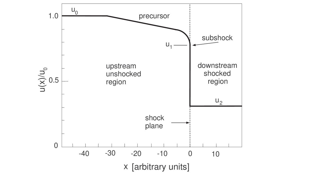
Figure 6.1: Idealized modified shock velocity profile with the main shock having compression ratio $r=u_{0}/u_{2}$, showing the precursor formed from the backreaction of accelerated particles, and the unmodified subshock with compression ratio $r_{s}=u_{1}/u_{2}$. The velocities $u_{0}$, $u_{1}$, and $u_{2}$ are all normalized to $u_{0}$, and flow from left to right in the diagram.

Slower shocks are modified on a larger scale, as shown in Figure 6.2, because the energetic, highly relativistic particles have speeds much greater than the shock speed and many particles penetrate far into the upstream region, causing significant backpressure there. As the shock speed becomes more and more relativistic, downstream energetic particles scattering back towards the upstream are unlikely to cross the shock into the upstream region unless they lie within a critical angle $\theta_{0}\sim 1/\gamma_{0}$, as discussed in detail in section 5.1. Particles with trajectories at larger angles are scattered back downstream without crossing the shock (Refer to Figures 5.8 and 5.9). Hence, fewer energetic particles cross the shock from downstream to upstream, the backpressure from energetic particles is lower and the highly relativistic shocks are modified on a smaller scale, as shown in Figure 6.2 as the dotted line.

Figure 6.2: Two modified shock velocity profiles with Lorentz factors of 1.25 and 8.0 as seen from the shock frame. The profile sharpens as the shock becomes more relativistic. The subshock is at $u_{1}$. The downstream flow velocity, $u_{2}$, is determined by the compression ratio which varies, depending on the speed of the shock. The shock is always modified in such a way as to conserve momentum and energy flux across the shock.

As a result, the modified velocity profiles of highly relativistic shocks appear to be much sharper than the velocity profiles of mildly relativistic shocks when viewed with the same distance scale.

The smoothing of the shock in the precursor region is such that the momentum and energy flux are conserved across the shock as shown in Figure 6.3. This plot was created by allowing a large number of particles to run through the Monte Carlo model with a shock speed Lorentz factor of 5 and compression ratio of 3.1. The model ran through a number of iterations, and after each iteration the model compared the flux on both sides of the shock (actually on both sides of every grid zone, both upstream and downstream) where the flux differences were noted and used to slightly adjust the shock velocity profile. If the correct compression ratio is used, the momentum and energy flux differences will be negligible after the last iteration and the fluxes will appear flat over the entire range of $x$ values, shown as the solid lines in the second and third frames of Figure 6.3. The dashed lines, representing the first iteration and the unmodified shock, show how bad the mismatch is in momentum and energy flux across the shock. Momentum and energy are not conserved in an unmodified shock when real particles are accelerated. Details of the shock modification method can be found in section 4.3.

Figure 6.3: The shock velocity profile for a modified shock (solid lines) with no subshock, and Lorentz factor $\gamma_{0}=5$, plus the corresponding momentum and energy flux profiles displayed on logarithmic scales. These may be compared with momentum and energy flux profiles for the unmodified shock (dashed) where the fluxes are not conserved across the shock.

6.2 Sensitivity of lepton momentum flux distributions to subshock size

To determine the sensitivity of lepton injection and acceleration characteristics to the size of the subshock in the shock velocity profile for mildly relativistic shocks, subshocks of various sizes were explicitly constructed with an input parameter as fractions of the difference between the $u_{0}$ and $u_{2}$ flow speeds. After the subshock sizes were chosen, the shocks were smoothed, either manually or with a combination of iterative smoothing, to insure that momentum and energy fluxes were conserved, as shown in Figure 6.3.

Manual smoothing means that a smoothing value was set as an input parameter. An algorithm in the Monte Carlo model uses this parameter to create exponential smoothing of the shock velocity profile into the upstream region. The model generates momentum and energy flux values at every grid zone based on the amount of smoothing introduced. After observing the resulting flux profiles and their deviation from a straight line across the shock (which means a deviation from the conservation of momentum and energy), the input smoothing value is adjusted and the model is rerun, one iteration at a time, until an acceptable flatness of the momentum and energy flux profiles is achieved, similar to the solid line in Figure 6.3. The manual method is less efficient and sometimes not as accurate as the automatic iterative method that the Monte Carlo model uses to adjust the velocity profile at every grid zone. However, manual smoothing is necessary at high Lorentz factors because the flux differences between grid zones become too small and the automatic smoothing becomes less accurate.

“Leptons” (i.e., particles chosen to have mass $m_{e}/m_{p}=0.1$, $0.01$ and $0.001$) were used for this study. Electrons with their actual mass were not used due to computer run time limitations. Referring to Figure 5.1 and the related text, the Monte Carlo model simulates pitch angle scattering by altering the momentum direction of a particle through a small random angle $\delta\theta$ (which depends on the particle’s gyroradius) in a small increment of time, $\delta t$. The result is that lighter particles with smaller momenta and smaller gyroradii require many more time steps to accomplish the same amount of scattering as heavier particles, roughly as the inverse ratio of the masses. Hence, computer runs using very small mass particles become excessively long, given the present CPU speeds that are available. Therefore, the strategy was to use three larger lepton masses to expeditiously generate data, and then extrapolate the results down to those for the mass of the electron. The results are straightforward and shown in Figure 6.7.

6.2.1 Lepton flux distributions

Momentum or energy flux distributions provide insight into how the particles are interacting with the shock and undergoing Fermi acceleration. The momentum flux distribution is measured by keeping track of the particles that cross a chosen boundary with the momentum associated with each particle, similar to the flux measurement at every grid zone as described in (Ellison & Reynolds, 1991). But, rather than simply summing the total flux in the $x$ direction, the momentum for the flux distribution is made to be omnidirectional with a cosine function and is sorted into bins depending on the magnitude of the momentum. The result is a plot of the momentum flux distribution, $f(p)$, as a function of momentum, $p$. Figure 6.4 shows a momentum flux distribution of particles with three different masses accelerated by an unmodified shock. An unmodified shock implies that the subshock size is the same size as the main shock, and implies that the entire shock width is much smaller than the diffusion length of all particles in the system, therefore particles of all energies (determined by the input parameters) can be accelerated by the shock. Also, because all particles see the same entire shock width, the momentum fluxes all have the same slope.

In the top frame of Figure 6.4, the momentum flux distributions $f(p)\propto p^{-\sigma}$, i.e., equation (1.12), of accelerated baryons and leptons are shown simply as the logarithms of $f(p)$ vs $p$. Their slope is called the spectral index, $\sigma$. In the bottom frame, the distributions are flattened by multiplying them by $p^{\sigma}$, which allows more direct comparisons of subtle variations in the momentum distributions. The point here is to show the concept for unmodified shocks, and the flattening will become more useful for modified nonlinear shocks to be discussed later.

As the particles scatter back and forth across the shock, they pick up increments of momentum, depending on their pitch angle at the time of crossing. Recalling the discussion at the beginning of this chapter, all particles pick up average energy of $\gamma_{\mathrm{rel}}mc^{2}$ and average momentum of $\gamma_{\mathrm{rel}}mv_{\mathrm{rel}}$ at the first shock crossing, hence the more massive particles initially have, on the average, more momentum than less massive particles in the ratio of their masses. For any given particle speed, the probability of return of the particle from downstream depends almost entirely on the compression ratio across the shock. Since all particles have the same probability of return for a given particle speed, the momentum distributions as a function of momentum will all have the same slope, as described in section 1.2. However, the distribution flux levels for the species were set at the earliest stages of acceleration, referring to equation (1.11), and they follow their corresponding flux levels for all higher momenta. For example, in the top frame of Figure 6.4, the less massive leptons (i.e., $m_{e}=0.1$ and $0.01$) scatter and accelerate at lower momenta with initially large momentum flux [again, equation (1.11)], but due to the constant spectral index, there are significantly fewer leptons and correspondingly lower lepton momentum flux at the initial momentum of accelerated baryons.

Figure 6.4: Spectra for an unmodified relativistic ($\gamma_{0}=2$) shock. The baryon and lepton spectra have the same slope, indicating that all particles have a sufficient diffusion length to interact with the shock. The bottom frame shows the same spectra, but flattened by multiplying the distribution function by normalized momentum raised to the power of $\sigma$.

Referring to Figure 6.2, shocks modified by the backpressure of energetic baryons are smoothed and the size of the subshock is correspondingly reduced to $u_{1}$. As a consequence, the less massive leptons, with initially less momentum and shorter diffusion lengths than baryons, cannot interact effectively with the entire shock because the shock is smoothed on the longer scale of the baryons. As a consequence, far fewer leptons reach energies where their diffusion lengths are comparable to those of baryons and the overall lepton flux is much lower. This effect can be observed in Figure 6.5. The leptons with mass $m_{e}=0.01$ are affected much more drastically than the leptons with mass $m_{e}=0.1$ by the smoothed shock.

Figure 6.5: Spectra for the modified relativistic ($\gamma_{0}=5$) shock shown in Figure 6.3. The baryon and lepton spectra develop the same slope, indicating that the leptons have achieved a long enough diffusion length to interact with the entire modified shock, but at greatly reduced numbers compared to baryons. The bottom frame shows the same spectra, but flattened by multiplying the distribution function by normalized momentum raised to the power of $\sigma$.

To determine the sensitivity of the lepton momentum flux to the size of the subshock, subshocks of various sizes were explicitly constructed with an input parameter, as described above, in smoothed shocks with various Lorentz factors. The subshock size is defined in the following way. Referring to Figure 6.1 again, the subshock fraction of the main shock is $f_{s}=(u_{1}-u_{2})/(u_{0}-u_{2})$. The compression ratio of the subshock is $r_{s}=u_{1}/u_{2}$ and the compression ratio of the main shock is $r=u_{0}/u_{2}$; hence, $f_{s}=(r_{s}-1)/(r-1)$, and $f_{s}$ is the normalized or relative subshock size. Subshock size can also be stated simply by just comparing compression ratios, $r_{s}/r$; however, this method gives a value of $1$ when the subshock disappears at $u_{1}=u_{2}$ and does not show the fraction of the main shock ascribed to the subshock.

The velocity profiles containing constructed subshocks were adjusted to conserve momentum and energy fluxes, using baryons only. The resulting velocity profiles were then used as a template to run the model with pairs of particle species, the first being baryons with mass equal to $1.0$ and the second being lighter particles with mass of either $0.1$, $0.01$, or $0.001$, each with its own number density of 1 particle per cubic centimeter. Little error was introduced by this method because the baryons are primarily responsible for the shock smoothing, and the smaller mass leptons were shown to have only a minor effect on the overall shock velocity profile smoothing and the related momentum and energy flux conservation profiles when the densities of baryons and leptons are approximately equal.

After each run was completed, the flux spectra was generated and measured from plots similar to the one shown in the bottom frame of Figure 6.5. The vertical axes of the plots show the logarithms of the fluxes, therefore the differences of the measured values between baryons and the lighter leptons directly give the logarithm of the ratio of their flux distributions, $log_{10}[f(e)/f(p)]$. A number of subshock sizes were explored, from $f_{s}=0$ to $f_{s}=0.8$, for several shock speeds with Lorentz factors ranging from $\gamma_{0}=2$ to $\gamma_{0}=12$. The results, shown in Figure 6.6, indicate a great increase in sensitivity to subshock size as the particles become less massive, but show little sensitivity to shock speed for the larger subshock sizes over the range studied here. For large subshock size, the flux values approach those of an unmodified shock, such as those shown in Figure 6.4. For small subshock size, lepton flux is extremely small and, as shown in Figure 6.7, with projections to the electron rest mass, $m_{e}/m_{p}=1836$, electrons would require a significant subshock size, or would need to be initially pre-energized by some other means, in order to enter into the first-order Fermi shock acceleration process. However, highly relativistic shocks tend to become very sharp on the scale of baryon diffusion lengths, as shown in Figure 6.2, and, for ultrarelativistic shocks, may be sharp on the scale of electron diffusion lengths and thereby have a large effective subshock capable of accelerating electrons. This may be the reason that there appears to be little dependence on shock speed when the constructed subshock is made large.

Figure 6.6: The ratio of lepton to baryon momentum flux as a function of subshock size is shown for particles with masses of $0.1$, $0.01$, and $0.001$. The lighter leptons are far more sensitive to subshock size than the heavier lepton, spanning fifteen orders of magnitude for small subshocks. Sensitivity to shock speed is low except for very small subshocks where the flux is seen to increase with higher Lorentz factors.

Figure 6.7: Projections of lepton flux from larger lepton masses down to the mass of the electron show what flux to expect for real electrons. Note that the subshock sizes are in terms of the compression ratios, $r_{s}/r$.

6.2.2 Lepton injection efficiency

The lepton momentum flux is directly related to the injection efficiency of leptons taking part in the first-order Fermi acceleration process. Based on the concept expressed by Ellison, Baring, & Jones (1995), the relative injection efficiency, $\epsilon_{\mathrm{inj}}(p>p_{0})$, can be defined as the number density of particles accelerated above a critical momentum, $p_{0}$, compared to the number density of particles $n_{0}$ flowing toward the shock, or

$$\epsilon_{inj}(>p_{0})\equiv\hbox{${{\displaystyle n_{\mathrm{inj}}(p>p_{o})\vphantom{(}}\over{\displaystyle n_{0}\vphantom{(}}}$}\ .$$ (6.1)

The critical momentum, shown as the dotted line in Figure 6.8, is approximately at $p/m_{p}c=5$ (i.e., $\mathrm{log}_{10}[p/m_{p}c]\approx 0.7$). This is the momentum where the thermal distribution of baryons ends and the power law distribution begins. The same momentum can be found in the lower frame of Figure 6.5 at the beginning of the flat portion of the baryon flux distribution and where all three momentum flux distributions flatten to the same power law for this particular case of a modified relativistic shock with Lorentz factor of $\gamma_{0}=5$. The efficiencies of each type of particle was normalized to 1.0 to allow the injection efficiency of each type to be measured against its own initial particle density. This also allows direct comparisons between injection efficiencies of the various particle types.

The injection efficiencies for leptons and baryons may be determined as follows. By using the critical momentum, $p_{0}$, as the defining point for baryons, the absolute injection efficiency for baryons is read off the plot shown in Figure 6.8. Then, using the same momentum, for leptons, the relative injection efficiencies for leptons are the differences (in logarithms) between the lepton efficiencies and the absolute baryon efficiency at $p_{0}$.

The critical momentum was found for each subshock size and for each Lorentz factor to provide the absolute injection efficiencies for baryons. Then, all of the relative injection efficiencies were found for leptons with masses of $0.1$, $0.01$, and $0.001$ to create the injection efficiencies shown as a function of fractional subshock size, $f_{s}$, in Figure 6.9. The lepton efficiencies are normalized to the baryon injection efficiency, and the baryon efficiency is shown as the absolute efficiency on the same graph. The normalization factor is the ratio of the baryon to lepton densities, taken in pairs. The injection efficiencies tend to follow the same pattern as did the fluxes. This is expected because the fluxes above the critical momentum generally follow the same power law for all particles. It may be noted in Figure 6.9 that the lepton injection efficiencies tend toward those of test particles in unmodified shocks (i.e., where $f_{s}=1$) at the highest subshock sizes at all shock speeds used in this study.

Figure 6.8: Injection efficiency $\epsilon_{inj}(>p)$, i.e., the fractional number density of particles above a given momentum, is plotted against normalized momentum. The critical momentum, $p_{0}$, is chosen at the point where baryons clearly obtain a power law dependence. Lepton power law dependence is also established around $p_{0}$.

Figure 6.9: The top curve shows the absolute injection efficiency of baryons in modified shocks as a function of subshock size. The curves for $m_{e}=0.1$, $0.01$, and $0.001$ are the relative injection efficiencies normalized to the baryon injection efficiency. The injection efficiencies tend to be higher for higher $\gamma_{0}$ shocks when the subshock is small.

Also note, at the smallest subshock sizes, there is a greater dependency on shock speed. This characteristic is shown more clearly in Figure 6.10. This figure shows the relative injection efficiency for leptons with masses $0.1$ and $0.01$ as a function of shock speed in shocks where there was no explicit subshock established. For the shock speeds with Lorentz factors of $2$ - $20$, there is a dramatic improvement in lepton injection efficiency through eight orders of magnitude in the $m_{e}/m_{p}=0.01$ mass. Shock speed dependence occurs because, as the speed increases, the shock front becomes sharper on the length scale of the lepton and more of the lower energy leptons can enter into the acceleration process. Once a particle reaches a momentum where its diffusion length is large enough to interact with the entire smoothed shock width (i.e., through the entire precursor region in Figure 6.1), the power law portion of the flux distribution curve begins and the injection efficiency is established.

Figure 6.10: Relative injection efficiency, normalized to baryon injection efficiency, increases with shock speed if there is no subshock. Leptons with mass $m_{e}/m_{p}=0.01$ may reach their maximum injection efficiency above a Lorentz factor of $\sim 100$.

Baryons reach this “critical momentum” point easily, compared to leptons. Lepton momentum is lower than baryon momentum at the same speeds due to their smaller masses. At shocks with low Lorentz factors, the diffusion lengths of all leptons increase substantially after the first crossing, but not enough to interact with the entire smoothed shock width. Leptons require additional shock crossings to reach the required energies to interact with the entire shock width and far fewer leptons can accomplish this, therefore the lepton injection efficiency is lower. The theoretical maximum relative injection efficiency would occur when the shock front is so narrow that the diffusion lengths of all particles, leptons included, is greater than the shock width after the first crossing. By the same argument presented earlier, the ratio of lepton to baryon momenta is lower by the ratio of their masses after the first crossing. Then, given equal number densities of leptons and baryons, the maximum relative injection efficiency of leptons depends only on the injection efficiency power law through the relation

$$\mathrm{log}_{10}[\epsilon_{\mathrm{inj}}(\mathrm{max})]=\sigma_{\mathrm{inj}}\mathrm{log}_{10}\hbox{${{\displaystyle m_{e}\vphantom{(}}\over{\displaystyle m_{p}\vphantom{(}}}$}\ .$$ (6.2)

The average measured $\sigma_{\mathrm{inj}}\sim 1.3\pm 0.1$. Computer results for leptons with mass $m_{e}/m_{p}=0.01$ extend only to a Lorentz factor of $20$, therefore it is not clear how their injection efficiency behaves at higher shock speeds, but based on the relationship above, the maximum relative injection efficiency for these particles may be approximately $10^{-2.6}$ at some Lorentz factor above $100$ in Figure 6.10. It appears that the maximum relative injection efficiency (i.e., at the same momentum) of leptons will always be far below that of baryons when their number densities are equal.

6.3 Characteristics of increased lepton densities

Injection efficiencies, as defined in the previous section show the fraction of particles that are incorporated into the Fermi acceleration process, but a more important question is how much energy is carried by the particles. Present gamma-ray burst models require leptons to carry a significant fraction of the total energy density of the burst, and there are a number of ways this cound occur. One possibility is through rapid energy transfer from baryons to leptons by some unknown means. Another possibility is through a mechanism other than shocks to directly energize leptons; for example, magnetic reconnection. The possibility that seems most likely, and the one that will be investigated here, is that there are more leptons than baryons, and they are energized by diffusive shock acceleration. One of the requirements in the Fireball model of a gamma-ray burst is that the baryon mass fraction must be low to allow the fireball to expand relativistically (e.g., Mészáros & Rees, 1997). In addition, in the Fireball model large numbers of electron-positron pairs are produced. This suggests that the energy is carried predominately by the leptons due to their large particle number density. In this section, the characteristics of energy distributions are explored for various lepton to baryon particle number density ratios.

Clearly, the energy carried by particles is in the ratio of their masses for particles with the same velocity. It was shown that when the leptons and baryons have equal particle densities, the baryons, and in particular the highly accelerated ones, carried significant energy and exerted the predominant backpressure on the shock to modify its velocity profile. As the lepton to baryon density ratio increases, the situation changes. Large numbers of leptons, compared to baryons, begin to exert their own backpressure on the shock velocity profile. Referring to Figure 6.11, for a lepton density a little higher than the baryon density, say for a case where $n_{e}/n_{p}\sim 10$, the shock velocity profile is still dominated by baryon momentum and the smoothing takes place on the scale of the baryon’s gyroradius. However, when leptons dominate, as is the case of a lepton to baryon density ratio of $10^{4}$ and a lepton mass of $0.01m_{p}$, the smoothing results more from the backpressure of the energetic leptons and on the scale of the lepton gyroradius, recalling that smoothing always occurs in such a way as to conserve momentum and energy flux across the shock. The resulting smoothed shock has a shock width very small on the scale of the baryon diffusion length, and is on the order of the lepton diffusion length. Leptons now interact with the shock as baryons did when baryon momentum was dominant. Clearly, all baryons returning from downstream see the entire shock width.

Figure 6.11: Velocity profiles steepen with increased lepton/baryon particle density ratios. The profile for a lepton density of $10^{4}\ \mathrm{cm}^{-3}$ with a lepton mass of $0.01m_{p}$ is also smoothed, but on the scale of the lepton gyroradius and therefore it appears very sharp to baryons, whose gyroradius is used here for units on the horizontal axis.

In Figure 6.8, the relative injection efficiency was defined at the onset of the power law for baryons, and a critical momentum $p_{0}$ was used to define the lepton injection efficiency because the lepton power law started at approximately that point. In other words, few leptons received enough initial momentum after the first crossing to return for additional acceleration and develop the power law. The leptons that remained had to undergo repeated accelerations to develop enough momentum with their related diffusion length to see the entire shock, hence the momentum flux of leptons in the power law region was very low, due to both their small mass and relatively few particles remaining, compared to baryons. This definition of (relative) injection efficiency is somewhat misleading when the shock front becomes narrow on the scale length of most particles, and this situation occurs when the lepton to baryon number density ratio increases beyond $10^{3}$. As leptons begin to have more influence over the shock modification and carry more total energy, and as the shock sharpens as shown in Figure 6.11, far more leptons can enter into the shock acceleration process after the first shock crossing. In other words, after the first shock crossing, the diffusion length of a much larger population of leptons extends over the entire lepton-modified shock width and the leptons start their power law, as shown in Figure 6.12 at point $a$. Point $a$ is determined by the ratio of the masses because after the first crossing, as discussed earlier, the average speed for all particles is $v_{\mathrm{rel}}$ and the momentum of a particle is $\gamma_{\mathrm{rel}}mv_{\mathrm{rel}}$.

Figure 6.12: Initial injection efficiencies are shown at $a$ for leptons and at $b$ for baryons after the first shock crossing of each species in a scenario where leptons dominate baryons by $10^{4}$. Due to the narrow or sharp shock, modified primarily by leptons, the injection efficiencies of all particles is relatively high and leptons achieve a power law after the first crossing, similar to baryons. Note that the baryon data were normalized by multiplying by the $n_{e}/n_{p}$ ratio.

All baryons have a sufficient diffusion length to see the entire shock and a large population of leptons can now see the entire shock. Therefore, both baryons and leptons have the same power law dependence after the first crossing and the relation, $p_{a}/p_{b}=m_{e}/m_{p}$ results, as shown at the top of Figure 6.12. This point becomes well defined and takes the shape of the baryon injection efficiency plot as the lepton to baryon density ratio continues to increase. The initial particle injection efficiency (i.e., in those cases where the power law begins after the first shock crossing) is defined as points $a$ and $b$. Defining the initial injection efficiency in this way indicates that the lepton and baryon particle injection efficiencies are nearly equal in Figure 6.12, but they occur at different momenta as mentioned above. In the previous section the mass difference was tied to the maximum relative injection efficiency through equation (6.2). Now the initial injection efficiency is connected to the maximum relative injection efficiency through this equation.

In order to make comparisons between lepton and baryon flux characteristics, they need to be measured at the same momentum, therefore the relative injection efficiency will be used as before, by taking the differences in logarithms between the lepton and baryon curves along the critical momentum line at $p_{0}$ (i.e., the momentum at point $b$ in Figure 6.12). This was done for a range of lepton to baryon particle number densities and for a range of shock speeds, using a lepton to baryon mass ratio of $0.01$. The results are expressed in Figure 6.13 as the ratio of lepton to baryon energy flux as a function of lepton to baryon particle number density. When the particle number density is low, flux characteristics are dominated by baryons and the baryon-smoothed shock. As the leptons become more important and the shock smoothing begins to be influenced by leptons as well as baryons, leptons begin to share more of the energy density, and eventually there will be a point where the leptons and baryons share energy equally. This point, on the equipartition line in Figure 6.13, appears to be at approximately $n_{e}/n_{p}\sim 1600$ for a lepton mass of $0.01m_{p}$. In other words, as the lepton to baryon particle number density increases from $\sim 10^{3}$ to $\sim 10^{4}$, the spectral characteristics of shock accelerated baryons and leptons with mass $m_{e}=0.01m_{p}$, and the shock profile itself, makes a transition from those dominated by baryons to those dominated by leptons. At higher number density ratios, both leptons and baryons behave the same. Leptons dominate completely above a number density ratio of about $10^{4}$ and, from that point on, the energy flux is simply proportional to the number density, hence the straight line (with a slope of 1).

Figure 6.13: Partitioning of energy among leptons and baryons as a function of the relative number density of leptons. The energy density is split equally between leptons of mass $0.01m_{p}$ and baryons when lepton density exceeds baryon density by approximately 1600. Leptons with the rest mass of the electron reach equipartition at a density ratio of $3.2\times 10^{5}$.

Additional energy fluxes were found at a number density ratio of $10^{6}$ for lepton masses of $0.1m_{p}$ and $0.001m_{p}$, and from these a projection was possible down to the electron mass of $(1/1836)m_{p}$. Straight lines, each with a slope of 1, can be projected back to the equipartition line and, if this is done for the electron mass (designated as the solid star in Figure 6.13, it can be estimated that the equipartition point for particles having the rest mass of an electron is at a lepton to baryon particle number density ratio of $3.2\times 10^{5}$. The measurements were collected from shocks with Lorentz factors of $2$ and $12$, the range of shock speeds in this study, and the results appear to be independent of these shock speeds above the equipartition line.

These concepts are expressed in a different way in Figure 6.14. Here, fractional total energy above momentum $p$ is shown for leptons and baryons for the case of relatively small lepton to baryon density in the top frame, and for a large lepton to baryon density in the lower frame. In the top frame, baryons carry the bulk of the total energy, even though lower in particle number because they entered into the acceleration process early and have a much higher density of accelerated particles as a result of baryons still dominating the shock smoothing. In the lower frame, leptons dominate the shock smoothing, also enter the acceleration process early, have a much higher density of accelerated particles (compared to leptons in the top frame) and, by their sheer numbers, now carry the bulk of the energy. In Figure 6.14, the curves are not normalized because the point here is to emphasized the actual fraction of total energy that is associated with each particle type.

Figure 6.14: Fraction of total kinetic energy carried by baryons and leptons is shown for two lepton to baryon density ratios. In the top frame where the lepton density is 100, the kinetic energy carried by leptons is up to four orders of magnitude below the faction carried by baryons. When the lepton density increase to $10^{6}$, as shown in the lower frame, the fraction of energy carried by leptons dominates.

Noting the vertical dotted line in Figure 6.14, another parameter can be defined as energy efficiency (sometimes called acceleration efficiency as it was defined in section 5.3.3), similar to what was done in Figure 6.10. Energy efficiency is the fraction of total energy remaining above momentum p. Since the dotted line in Figure 6.14 is chosen, as before, at the onset of the power law portion of the baryon curve, this momentum is also the critical momentum, $p_{0}$. Hence, energy efficiency (or acceleration efficiency) is

$$\epsilon_{\mathrm{acc}}(p>p_{0})\equiv\hbox{${{\displaystyle\mathrm{fraction\ of\ total\ kinetic\ energy\ density\ above}\ p_{0}\vphantom{(}}\over{\displaystyle\mathrm{total\ kinetic\ energy\ density}\vphantom{(}}}$}$$ (6.3)

Using this definition, ratios of the energy efficiencies can be measured for various lepton baryon density ratios and for various shock speeds, similar to what was done for injection efficiencies. These results were compiled for a lepton mass of $0.01$. When they are plotted on the same graph in Figure 6.13, they overlay the $m_{e}=0.01$ curve exactly, and this is not surprising. Injection efficiency and energy efficiency are closely related because injection efficiency is concerned with the fraction of particles that get injected into the acceleration process and energy efficiency is concerned with the fraction of kinetic energy carried by these same particles. Since they were defined at the point where each curve entered the (constant) power law dependence, the most they could vary is by a constant. The constant is $1$.

6.4 Summary

Leptons with various masses and baryons were subjected to a range of plane parallel modified shocks having Lorentz factors from $2$ up to $20$. The energy and momentum fluxes of these particles were studied as a function of unmodified subshock size and particle number density to try to better understand the parameters required for leptons to carry a significant portion of the energy in a gamma-ray burst.

Assuming equal numbers of leptons and baryons, baryons dominate the shock smoothing process and lepton injection efficiencies are very sensitive to the size of any embedded subshock, the sensitivity increasing with decreasing lepton mass.

For subshock fractional sizes, $f_{s}$, above $0.4$, the injection efficiencies of leptons appear to be insensitive to shock speeds over the range used in this study. In the case of negligible subshock, the injection efficiencies of leptons are sensitive to the shock speed, and projections suggest that for shock Lorentz factors on the order of $100$, the shock front may be sufficiently narrow to increase the relative injection efficiency of leptons with mass $0.01m_{p}$ to a maximum of $10^{-2.6}$ of the baryon injection efficiency. A lepton mass of $m_{e}\sim(1/1836)m_{p}$ may require a shock Lorentz factor greater than $1000$ to reach a maximum relative injection efficiency of about $10^{-4.2}$ that of baryons. The overall conclusion is that, given the assumptions in the Monte Carlo model, leptons can never carry enough energy to explain the spectra observed in gamma-ray bursts if the lepton to baryon particle densities are of the same order, even for ultrarelativistic shock speeds.

The injection efficiencies of leptons and baryons were studied in the case where the lepton to baryon number density ratios were varied and a lepton to baryon mass ratio of $0.01$ was used. It was found that, as expected, for low number density ratios, baryons dominate the shock smoothing and the lepton injection efficiencies and energy efficiencies remained low. As the number density ratio increased to the $10^{3}$ range, leptons began to have a strong influence on the modification of the shock velocity profile, the shock became much sharper, and a much larger population of leptons were injected into the shock process. The energy equipartition point of leptons with mass of $0.01m_{p}$ was at the particle number density ratio of $1600$. Above a number density ratio of $10^{4}$, leptons were found to dominate the shock smoothing process and the energy flux was directly proportional to number density ratio. Using this method, an extrapolation was made down to the mass of the electron, and it was determined that the energy equipartition point for electrons (and positrons) in plane parallel shocks is at a lepton to baryon number density ratio of $3.2\times 10^{5}$. This result was independent of shock speeds with Lorentz factors of $2$ to $12$ used in this study. However, the energy equipartition point may be independent of shocks with any higher Lorentz factor for the following reason. When the lepton to baryon particle densities are of the same order, the maximum lepton relative injection efficiency occurs at ultrarelativistic shock speeds and it is far below baryon injection efficiency (at the same momentum). Hence, the only way the lepton efficiency can dominate, under the same acceleration assumptions, is by increasing the lepton to baryon number density ratio. When the lepton density ratio is high enough that leptons dominate the shock modification process, shock speed no longer plays a roll in increasing injection efficiency. The high number density ratio of leptons to baryons is required for two reasons. The low mass of the leptons means that each lepton carries far less energy than baryons, in proportion to their masses at the same speeds, therefore large numbers of leptons are necessary to carry an equal portion of the total energy. More importantly, there must be a sufficient lepton density to dominate the shock smoothing so that larger numbers of leptons can be injected into the shock acceleration process.

The primary finding in this study was that for plane modified shocks with the magnetic field parallel to the shock normal, and with shock Lorentz factors in the $2$ to $12$ range, the particle number density ratio between leptons and baryons must be above $3.2\times 10^{5}$ for leptons with the rest mass of the electron to carry sufficient kinetic energy in gamma-ray bursts and account for the observed GRB spectra. The energy equipartition point appears to be independent of shock speed.

Chapter 7 Conclusions

Chapter summaries can be found at the end of each chapter, but the accomplishments and main conclusions of the entire dissertation are summarized here. Despite the fact that relativistic shock theory has concentrated almost exclusively on test-particle acceleration, it is likely that relativistic shocks are not test-particle but inject and accelerate particles efficiently. The reason is that regardless of the ambient far upstream conditions, all particles that are overtaken by a relativistic shock will receive a large boost in energy $\Delta E\sim\gamma_{\mathrm{rel}}mc^{2}$ in their first shock crossing. Thus, virtually all of the particles in the downstream region of an unmodified shock are strongly relativistic with $v\sim c$. The ability to overtake the shock from downstream and be further accelerated depends only on the particle speed (Eq. 5.7), the presence of magnetic waves or turbulence with sufficient power in wavelengths on the order of the particle gyroradii to isotropize the downstream distributions, and the pitch angle of the returning particle (Eq. 5.4). It is generally assumed that the necessary magnetic turbulence is self-generated and if enough turbulence is generated to scatter high momentum particles (with very low densities) that constitute a test-particle power law, there should be enough generated to isotropize lower momentum particles (which carry the bulk of the density). If acceleration can occur at all, it is likely to occur efficiently making it necessary to calculate the shock structure and particle acceleration self-consistently. Furthermore, if relativistic shock theory is to be applied to gamma-ray bursts, where high conversion efficiencies are generally assumed, nonlinear effects must be calculated.

When energetic particles are generated in sufficient numbers, the conservation of momentum and energy requires that their backpressure modify the shock structure. Two basic effects occur: a precursor is formed when the upstream plasma is slowed by the backpressure of the accelerated particles and the overall compression ratio changes from the test-particle value as a result of high energy particles escaping and/or a change in the shocked plasma’s adiabatic index $\Gamma$. As indicated by the $\gamma_{0}=1.4$ example (Section 5.3.1), mildly relativistic shocks act as nonrelativistic ones showing a dramatic weakening of the subshock combined with a large increase in $r$ (Fig. 5.10). These changes result in a particle distribution which is both steeper than the test-particle power law at low momenta and flatter at high momenta (Fig. 5.11).

In faster shocks (i.e., $\gamma_{0}\mathrel{\hbox{\hbox to0.0pt{\hbox{\lower 4.0pt\hbox{$\sim$}}\hss}\hbox{$>$}}}3$), the initial test-particle spectrum is steep enough that particle escape is unimportant so only changes in $\Gamma$ determine $r$ (Eq. 5.16). In contrast to nonrelativistic shocks where the production of relativistic particles causes the compression ratio to increase, it is shown that $r$ decreases smoothly to $3$ as $\gamma_{0}$ increases and the fraction of fully relativistic shocked particles approaches one (Fig. 5.6).

An important result is that efficient, mildly relativistic shocks do not produce particle spectra close to the so-called ‘universal’ power law having $\sigma\sim 4.23$. This may be important for the interpretation of gamma-ray bursts since the internal shocks assumed responsible for converting the bulk kinetic energy of the fireball into internal particle energy may be mildly relativistic and the external shocks, believed responsible for producing gamma-ray burst afterglows, will always go through a mildly relativistic phase (see Piran, 1999, for a comprehensive review of gamma-ray bursts).

7.1 Relativistic magnetohydrodynamic Monte Carlo model

The basic shock acceleration physics is independent of the speed of the shock, but the mathematical modeling of the shock process depends on whether or not particle speeds are large compared to the shock speed. The relativistic Monte Carlo model used for this study, allows particle speeds to be comparable to shock speeds and, aside from computational limits, the model allows shocks to have arbitrary Lorentz factors.

The fully relativistic nonlinear Monte Carlo model, under development from a nonrelativistic model, will simulate kinematic particle acceleration in steady-state modified shocks with a gyrotropic pressure tensor and magnetic fields at oblique angles when it is completed. In its present state, operating with the magnetic field parallel to the shock normal, the shocks can be self-consistently modified while conserving particles, momentum, and energy across the shock, and while allowing charged particles to gain energy by first-order Fermi acceleration, and escape when they reach a high enough energy. The model can also be used with oblique angles and anisotropic pressure for unmodified test particle shocks.

New flux conservation laws of energy and momentum were developed by setting the divergence of the stress-energy tensor equal to zero and applying the 4-dimensional version of Gauss’ theorem. Combining these equations with Maxwell equations yields a completely general set of relativistic magnetohydrodynamic jump conditions across the shock. A new equation of state was developed from the conservation of total energy that incorporates oblique magnetic fields and gyrotropic pressure. A new equation was developed from kinetic theory that gives an excellent approximation to the adiabatic index at intermediate shock speeds. The adiabatic index becomes the normal ratio of specific heats at the nonrelativistic limit ($5/3$) and at the ultrarelativistic limit ($4/3$). An anisotropy parameter was introduced for the gyrotropic pressure tensor to allow an analytic solution to the equations. The Monte Carlo code was further developed with new relativistic momentum transformation equations and a method of handling fluxes at grid zones for relativistic shock modification.

The Monte Carlo model was used first to duplicate well known test particle power law results in fully nonrelativistic and ultrarelativistic parallel shocks and was shown to move all parameters smoothly between these two shock speed regimes. The model was used in the trans-relativistic regime and can self-consistently determine compression ratios and adiabatic indices in close agreement with recent analytic results of Kirk et al. (2000). A number of solutions were presented where the downstream pressure is anisotropic. This is believed to be the first presentation of oblique shock solutions which apply smoothly for nonrelativistic, trans-relativistic, and ultrarelativistic shocks.

The results presented in Chapter 5 assumed that no first-order Fermi acceleration occurs, but they apply directly to test-particle acceleration where the energy density in accelerated particles is small. In that case, the differences in the compression ratio, $r$, produced by large magnetic fields and/or anisotropic pressures, even at ultrarelativistic speeds, become important since changes in $r$ map directly to changes in the power law index of the accelerated spectrum. This power law is the most important characteristic of test-particle Fermi acceleration and is often associated with ultrarelativistic internal shocks in gamma-ray burst (GRB) models. In standard GRB models, the rapidly expanding fireball cools, converting the internal energy of the hot plasma into kinetic energy of the relativistically moving ejecta and electron-positron pairs. At the point where the fireball becomes optically thin and the GRB we see is emitted, the matter is too cool to emit gamma-rays unless some mechanism can efficiently re-convert the kinetic energy back into random internal energy, i.e., unless some particle acceleration process takes place. Fermi shock acceleration is widely believed to be this mechanism (e.g., Rees & Mészáros, 1992; Piran, 1999).

Internal flows in GRBs may be ultrarelativistic, but when a fast flow overtakes a slower flow, the resulting shocks may be in the trans-relativistic range and may be responsible for the early transient gamma-ray intensity peaks. The outer blast wave shock slows as it sweeps up and accelerates interstellar material. This shock, believed to produce long-lasting afterglows, will eventually always go through a trans-relativistic phase, and the results apply to particle acceleration here as well.

7.2 Application to lepton and baryon acceleration

The Monte Carlo model was applied to lepton and baryon particle acceleration for the case of moderately relativistic, smoothed shocks with the shock normal parallel to the magnetic field. Using leptons of various light masses, and equal particle densities, it was found that unmodified subshocks of various fractional sizes within the main modified shock produced a large change in the lepton flux. The sensitivity to the larger fractional sizes of the subshock was little affected by the speed of the shock in the range of Lorentz factors between 2 and 12. However, in the case of no subshock, or small subshock, it was found that the lepton to baryon relative injection efficiency ratio, based on the critical momentum, $p_{0}$, where baryons start the power law distribution, increased substantially as the shock speed increased. For leptons with mass of $0.01m_{p}$ that of the baryon, leptons reach their maximum relative injection efficiency of approximately $10^{-2.6}$ that of baryons around a shock Lorentz factor of $100$. For a lepton mass of $m_{e}\sim(1/1836)m_{p}$, the shock Lorentz factor may need to be greater than $1000$ to reach a maximum relative injection efficiency of about $10^{-4.2}$ that of baryons. Such speeds may briefly occur in the initial outflow of a GRB, but it would require the entrained total baryonic mass to be very small (i.e., less than $10^{-4}M_{\odot}$; Rees, 2000). The conclusion here is that, given the assumptions of this model with particles energized by diffusive shock acceleration, leptons cannot carry sufficient energy to explain the observed spectra if the lepton and baryon densities are of the same order.

Present gamma-ray burst models require leptons to carry a significant fraction of the total energy density of the burst. The most likely possibility is that there are far more leptons than baryons. Arguments connected with opacity and variability timescales, etc (e.g., Piran, 1999) require highly relativistic outflow in GRBs and this is only possible if the total baryonic mass is low. If the total baryonic mass is low and if electron-positron pairs are created in large numbers by the initial gamma-ray photon burst while the burst is still opaque (Ramirez-Ruiz, MacFadyen, & Lazzati, 2002) and by neutrinos if the baryonic density is low (Rees, 2000), then lepton to baryon particle density ratio should be high. If it is high enough, then leptons can carry the bulk of the available burst energy.

The question then is what ratio of leptons to baryons would be required for equal sharing of the energy between the two species. The characteristics of leptons and baryons with various particle number densities were studied for plane parallel, relativistic, modified shocks in the same speed range. Initial energy and momentum of the particles, after the first shock crossing, was found to be in the ratio of their masses as expected. For moderately high lepton to baryon number density ratios (e.g., $10$ - $100$), the smoothed shock velocity profile modification was completely dominated by baryons. Using a lepton mass of $0.01m_{p}$, it was found that the shock and spectral characteristics make a transition from baryon dominated to lepton dominated in the lepton to baryon number density ratio range of $10^{3}$ to $10^{4}$. Leptons with mass $0.01m_{p}$ shared energy density equally with baryons when the particle number density ratio was approximately 1600. Above this point, leptons begin to completely dominate the energy and energy flux, and was found to be directly proportional to number density ratio.

By using leptons of various masses, a projection was possible down to the mass of the electron ($m_{e}/m_{p}\sim 1/1836$). An important and new result was that the energy density equipartition point between electron-positron pairs and baryons was at a lepton to baryon particle number density ratio of $3.2\times 10^{5}$, and it appears to be independent of the shock Lorentz factor. This suggests the possibility that, over a wide range of shock conditions, the number density ratio of leptons to baryons required for equipartition of kinetic energy in a GRB may stay roughly constant, similar to the constant value found above for parallel shocks.

After the Monte Carlo model is completed, the model will be used to further investigate lepton and baryon acceleration using oblique nonlinear shocks. This may better establish the lepton to baryon number density ratio required for equipartition.

Appendix A Definitions and Fundamental Relationships

Alfvén velocity

$v_{A}\propto\hbox{${{\displaystyle B\vphantom{(}}\over{\displaystyle\sqrt{\gamma\rho}\vphantom{(}}}$}$ where $B$ is the magnetic field strength, $\gamma$ is the pertinent Lorentz factor and $\rho$ is the rest mass density. The Alfvén velocity refers to the speed of propagation of a transverse magnetic disturbance along the direction of the magnetic field.

Gyroradius

$r_{g}=\hbox{${{\displaystyle p\vphantom{(}}\over{\displaystyle ZqB\vphantom{(}}}$}$ for charged particles in the presence of a magnetic field, where $p$ is the particle’s momentum, $q$ is the unit electric charge, $Zq$ is the particle’s total charge ($Z$ is the total charge number), and $B$ is the magnetic field strength.

Mean free path

$\lambda=\eta r_{g}$, is the average distance between collisions, if the particles undergo collisions. For collisionless interactions (e.g., through magnetic field tubulence), a similar concept can be defined as the average distance required for the particle to change direction by $90$ degrees. Bohm diffusion is assumed when the gyrofactor $\eta=1$. Higher values of $\eta$ imply smoother magnetic fields, less scattering, and longer mean free paths.

Diffusion coefficient

$\kappa=\hbox{${{\displaystyle 1\vphantom{(}}\over{\displaystyle 3\vphantom{(}}}$}\lambda v=\hbox{${{\displaystyle 1\vphantom{(}}\over{\displaystyle 3\vphantom{(}}}$}\eta r_{g}v=\hbox{${{\displaystyle 1\vphantom{(}}\over{\displaystyle 3\vphantom{(}}}$}\hbox{${{\displaystyle\eta pv\vphantom{(}}\over{\displaystyle ZqB\vphantom{(}}}$}=\hbox{${{\displaystyle 1\vphantom{(}}\over{\displaystyle 3\vphantom{(}}}$}\hbox{${{\displaystyle\eta\gamma\beta^{2}mc^{2}\vphantom{(}}\over{\displaystyle ZqB\vphantom{(}}}$}$, where $\beta$ is the speed of the particle.

Diffusion length

$L=\hbox{${{\displaystyle\kappa\vphantom{(}}\over{\displaystyle u_{0}\vphantom{(}}}$}=\hbox{${{\displaystyle 1\vphantom{(}}\over{\displaystyle 3\vphantom{(}}}$}\hbox{${{\displaystyle\lambda v\vphantom{(}}\over{\displaystyle u_{0}\vphantom{(}}}$}=\hbox{${{\displaystyle 1\vphantom{(}}\over{\displaystyle 3\vphantom{(}}}$}\hbox{${{\displaystyle\eta r_{g}v\vphantom{(}}\over{\displaystyle u_{0}\vphantom{(}}}$}\propto pv$, where $u_{0}$ is the shock speed.

Collision time

$t_{c}=\hbox{${{\displaystyle\lambda\vphantom{(}}\over{\displaystyle v\vphantom{(}}}$}=\hbox{${{\displaystyle\eta r_{g}\vphantom{(}}\over{\displaystyle v\vphantom{(}}}$}$ is a means of estimating the time for a particle to scatter through an angle of $90$ degrees.

Debye length

$\lambda_{D}\propto\sqrt{\hbox{${{\displaystyle E\vphantom{(}}\over{\displaystyle nq^{2}\vphantom{(}}}$}}$ is a measure of the electrostatic shielding distance around a charged particle in a plasma (Shu, 1992). $E$ refers to the kinetic energy of electrons, $n$ is the total particle number density, and $q$ is the unit electric charge.

Rigidity

$R=\hbox{${{\displaystyle pc\vphantom{(}}\over{\displaystyle Zq\vphantom{(}}}$}$ provides a measure of the sensitivity of the momentum of a particle to a magnetic field. The higher the rigidity, the less influence a magnetic field has on the path of the particle.

Energy and momentum flux distributions

distributions $f(p)$ or $g(E)$ are defined here as the total number of passages of particles through a grid plane from any direction.

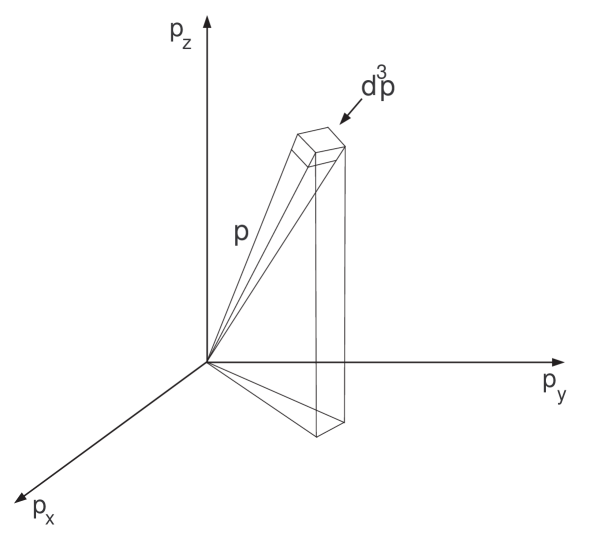
Figure A.1: Momentum space diagram showing an element of momentum space $d^{3}p$

Referring to Figure A.1, the total number of particles in momentum space is

$$\int_{-\infty}^{\infty}f(\vec{p})d^{3}p=4\pi\int_{0}^{\infty}p^{2}f(p)dp$$ (A.1)

provided the integration takes place where the distribution is isotropic; then

$$4\pi p^{2}f(p)dp\ \mathrm{gives\ the}\ \left[\hbox{${{\displaystyle\mathrm{\#\ \ of\ \ particles}\vphantom{(}}\over{\displaystyle\mathrm{cm^{3}}\vphantom{(}}}$}\right]\ \mathrm{in\ \ dp}$$ (A.2)

In the same way, if

$$\int_{0}^{\infty}g(E)dE=\hbox{${{\displaystyle 4\pi\vphantom{(}}\over{\displaystyle v\vphantom{(}}}$}\int_{0}^{\infty}\hbox{${{\displaystyle dJ\vphantom{(}}\over{\displaystyle dE\vphantom{(}}}$}dE$$ (A.3)

represents the total number of particles in energy space, where ${{\displaystyle dJ\vphantom{(}}\over{\displaystyle dE\vphantom{(}}}$ represents the differential flux in particles/($\mathrm{cm}^{2}\cdot\mathrm{second}\cdot\mathrm{ster}\cdot\mathrm{E}$), then

$$\hbox{${{\displaystyle 4\pi\vphantom{(}}\over{\displaystyle v\vphantom{(}}}$}\hbox{${{\displaystyle dJ\vphantom{(}}\over{\displaystyle dE\vphantom{(}}}$}dE\ \mathrm{gives\ the}\ \left[\hbox{${{\displaystyle\mathrm{\#\ \ of\ \ particles}\vphantom{(}}\over{\displaystyle\mathrm{cm^{3}}\vphantom{(}}}$}\right]\ \mathrm{in\ \ dE}$$ (A.4)

and the densities can be equated, yielding:

$$\hbox{${{\displaystyle dJ\vphantom{(}}\over{\displaystyle dE\vphantom{(}}}$}=vp^{2}f(p)\hbox{${{\displaystyle dp\vphantom{(}}\over{\displaystyle dE\vphantom{(}}}$}$$ (A.5)

Finally, using the relation $E^{2}=p^{2}c^{2}+(mc^{2})^{2}$, equation (A.5) simplifies to

$$\hbox{${{\displaystyle dJ\vphantom{(}}\over{\displaystyle dE\vphantom{(}}}$}=p^{2}f(p)$$ (A.6)

Appendix B Determining the ratio of specific heats

B.1 Kinetic pressure and the equation of state

The total distribution of particle momenta in a plasma gives the plasma a certain internal energy which has associated with it an adiabatic exponent or index. The discussion that follows develops a relationship between this adiabatic index and the calculated average momentum, or kinetic energy of the particles, based on simple statistical physics. The relationship can be used to estimate the adiabatic index in the downstream plasma frame of a relativistic shock. The concepts are well known and versions of the derivation below are found in most basic texts that discuss kinetic theory (e.g., Feynman, Leighton & Sands, 1963). This overview is for the convenience of the reader.

The adiabatic equation of state for an ideal gas of point particles, relating the pressure and volume of a closed system, may be written as

$$PV^{\Gamma}=C$$ (B.1)

where $P$ is the kinetic pressure, $V$is the volume under consideration, $\Gamma$ is the adiabatic index, and $C$ is a proportionality constant. The significance of point particles is that the particles have no rotational or vibrational contributions and all of the kinetic energy of the particles is due to translation.

Taking logarithms and then the derivatives in the equation above, one has

$$\frac{dP}{P}+\Gamma\frac{dV}{V}=0\qquad{\mathrm{o}r}\qquad VdP+\Gamma PdV=0$$ (B.2)

Adding $PdV$ to both sides and rearranging,

$$\frac{PdV+VdP}{\Gamma-1}=-PdV=dU.$$ (B.3)

Since $-PdV$ represents an adiabatic incremental compression of a volume at constant pressure and $dU$ is the corresponding increase in total internal energy, and since the left hand side has the total derivative of $PV$, one can integrate, with the appropriate limits, and write:

$$\frac{PV}{\Gamma-1}=U\qquad\mathrm{or}\qquad\frac{U}{V}=u=\frac{P}{\Gamma-1}.$$ (B.4)

where $u$ is the total internal energy density of the particle ensemble.

The exponent, $\Gamma$, is sometimes called the ratio of specific heats, but this is only accurate in the nonrelativistic ($\Gamma=5/3$) and ultrarelativistic ($\Gamma=4/3$) limits. Between these two limits, $\Gamma$ is simply the exponent for the adiabatic relation or the adiabatic index.

The total energy density $e$ and isotropic pressure $P$ are related through a combination of the adiabatic equation of state (i.e., equation (B.4) and the conservation of energy, which forms another equation of state:

$$e=\hbox{${{\displaystyle P\vphantom{(}}\over{\displaystyle\Gamma-1\vphantom{(}}}$}+\rho c^{2}$$ (B.5)

B.2 Nonrelativistic case

Consider a rigid rectangular chamber with a movable wall on the right end as shown in Figure B.1. The chamber contains ideal point particles of particle density $n$. The volume of the chamber has dimensions $x,y,z$ and the movable wall with area $A=yz$ on the right end is pushed into the volume a distance $-dx$ by a normal force $F$. Then the reversible work done on the volume is $dW=F(-dx)=PA(-dx)=-PdV$, where $-dV$ is the corresponding decrease in volume and P is the pressure inside the box.

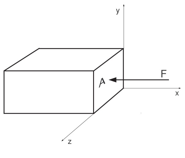
Figure B.1: A rectangular volume containing ideal particles under adiabatic compression from a force $F$.

The total momentum change by a particle moving in the $x$ direction inside the volume and elastically colliding with the movable wall is $\delta p=2p_{x}$. The total number of particles that collide with the movable wall in time $\delta t$ is $nv_{x}\delta tA$. Hence, the force on the movable wall inside the volume is $F=\hbox{${{\displaystyle\delta p_{tot}\vphantom{(}}\over{\displaystyle\delta t\vphantom{(}}}$}=(nv_{x}A)(2p_{x})$ and the pressure is $P=2np_{x}v_{x}$. The particle velocities have a wide range of speeds and directions and, in particular, only half the particles in the $x$ direction move toward the movable wall. Taking these considerations into account while averaging over the velocities, the pressure becomes $P=n<p_{x}v_{x}>$. If there are no magnetic fields and the $x,y\mathrm{\ and\ }z$ velocity distributions are equivalent, then $<p_{x}v_{x}>=\hbox{${{\displaystyle 1\vphantom{(}}\over{\displaystyle 3\vphantom{(}}}$}<\vec{p}\cdot\vec{v}>$, and the isotropic pressure can be written as

$$P=\hbox{${{\displaystyle 1\vphantom{(}}\over{\displaystyle 3\vphantom{(}}}$}n<\vec{p}\cdot\vec{v}>$$ (B.6)

It might be noted here, that if magnetic fields were present, one might take averages of the momenta parallel and perpendicular to the magnetic field, assuming rotational symmetry about the field vector. In that case one could have a gyrotropic pressure (tensor) with the following space components along the diagonal:

$$P_{\parallel}=n<\vec{p}\cdot\vec{v}>_{\parallel}$$ (B.7)

and

$$P_{\perp}=\hbox{${{\displaystyle n\vphantom{(}}\over{\displaystyle 2\vphantom{(}}}$}<\vec{p}\cdot\vec{v}>_{\perp}$$ (B.8)

In general, the momentum for a particle with mass $m$ and speed $v$ is

$$p=\hbox{${{\displaystyle\sqrt{E_{tot}^{2}-(mc^{2}})^{2}\vphantom{(}}\over{\displaystyle c\vphantom{(}}}$}=mc\sqrt{\gamma^{2}-1}=mc\sqrt{\gamma^{2}\beta^{2}}=\gamma mv$$ (B.9)

where the Lorentz factor $\gamma=(1-\hbox{${{\displaystyle v^{2}\vphantom{(}}\over{\displaystyle c^{2}\vphantom{(}}}$})^{-\frac{1}{2}}$.

Using this relationship for momentum one can write, for isotropic pressure,

$$P=\hbox{${{\displaystyle 1\vphantom{(}}\over{\displaystyle 3\vphantom{(}}}$}n\left<\gamma mv^{2}\right>\ .$$ (B.10)

For speeds where $\gamma\sim 1$, equation (2.6) can be approximated to first order as

$$P=\hbox{${{\displaystyle 2\vphantom{(}}\over{\displaystyle 3\vphantom{(}}}$}n\left<\hbox{${{\displaystyle mv^{2}\vphantom{(}}\over{\displaystyle 2\vphantom{(}}}$}\right>=\hbox{${{\displaystyle 2\vphantom{(}}\over{\displaystyle 3\vphantom{(}}}$}\hbox{${{\displaystyle U\vphantom{(}}\over{\displaystyle V\vphantom{(}}}$}\ ,$$ (B.11)

where $U$ is the total internal energy and is the total kinetic energy of ideal point particles in the volume under consideration.

Comparing equation (B.11) to equation (B.4) above, it can be seen that $\Gamma-1$ corresponds to ${{\displaystyle 2\vphantom{(}}\over{\displaystyle 3\vphantom{(}}}$, which yields $\Gamma=\hbox{${{\displaystyle 5\vphantom{(}}\over{\displaystyle 3\vphantom{(}}}$}$. This is the value for the adiabatic ratio of specific heats for ideal point particles having nonrelativistic speeds where $\gamma\sim 1$.

An error is introduced if the expression $\gamma mv^{2}/2$ is interpreted to be kinetic energy at mildly relativistic speeds where the appropriate expression for kinetic energy should be $mc^{2}(\gamma-1)$. For example, a 0.1 per cent error occurs, and will continue to increase for $v\mathrel{\hbox{\hbox to0.0pt{\hbox{\lower 4.0pt\hbox{$\sim$}}\hss}\hbox{$>$}}}0.1c$. At $v\sim 0.6c$, the error increases to about five per cent.

B.3 Ultrarelativistic case

The same ideas can be used to derive an expression for isotropic pressure for ultrarelativistic particles in the volume described above, and the resulting relationship will be the same as in equation (B.6), i.e. $P=\hbox{${{\displaystyle 1\vphantom{(}}\over{\displaystyle 3\vphantom{(}}}$}n<\vec{p}\cdot\vec{v}>$. However, for true ultrarelativistic particles, the momentum of the particles is $p=\hbox{${{\displaystyle E_{tot}\vphantom{(}}\over{\displaystyle c\vphantom{(}}}$}$, kinetic energy $E_{k}=E_{tot}=\gamma mc^{2}$ and $v\sim c$. The equation for isotropic pressure becomes:

$$P=\hbox{${{\displaystyle 1\vphantom{(}}\over{\displaystyle 3\vphantom{(}}}$}n\left<\gamma mc^{2}\right>=\hbox{${{\displaystyle 1\vphantom{(}}\over{\displaystyle 3\vphantom{(}}}$}\hbox{${{\displaystyle U\vphantom{(}}\over{\displaystyle V\vphantom{(}}}$}$$ (B.12)

and by the same comparison, this time equation (B.12) to equation (B.4), $\Gamma-1=\hbox{${{\displaystyle 1\vphantom{(}}\over{\displaystyle 3\vphantom{(}}}$}$ and $\Gamma=\hbox{${{\displaystyle 4\vphantom{(}}\over{\displaystyle 3\vphantom{(}}}$}$.

An error is introduced if the ultrarelativistic case is assumed at less relativistic speeds where the rest mass cannot quite be neglected. For example, a 0.1 per cent error occurs, and will continue to slowly increase for Lorentz factors $\gamma\mathrel{\hbox{\hbox to0.0pt{\hbox{\lower 4.0pt\hbox{$\sim$}}\hss}\hbox{$<$}}}500$, but at $\gamma\sim 10$, the error has only increased to approximately five per cent.

References

- Achterberg et al. (2001) Achterberg, A., Gallant, Y. A., Kirk, J. G., & Guthmann, A. W., Particle acceleration by ultra-relativistic shocks: theory and simulations, 2001, M.N.R.A.S., 328, 393
- Appl & Camenzind (1988) Appl, S. & Camenzind, M., Shock conditions for relativistic MHD jets, 1988, A&A, 206, 258
- Axford, Leer, & Skadron (1977) Axford, W. I., Leer, E., & Skadron, G., The Acceleration of Cosmic Rays by Shock Waves, 1977, in Proc. 15th ICRC(Plovdiv), 11, 132
- Ballard & Heavens (1991) Ballard, K.R. & Heavens, A.F., First-order Fermi Acceleration at Oblique Relativistic Magnetohydromagnetic Shocks, 1991, M.N.R.A.S., 251, 438
- Bednarz & Ostrowski (1996) Bednarz, J., & Ostrowski, M., The acceleration time-scale for first-order Fermi acceleration in relativistic shock waves, 1996, M.N.R.A.S., 283, 447
- Bednarz & Ostrowski (1998) Bednarz, J. & Ostrowski, M., Energy Spectra of Cosmic Rays Accelerated at Ultrarelativistic Shock Waves, 1998, Phys. Rev. Letts, 80, 3911
- Bell (1978a) Bell, A. R., The Acceleration of Cosmic Rays in Shock Fronts - I, 1978a, M.N.R.A.S., 182, 147-156
- Bell (1978b) Bell, A. R., The Acceleration of Cosmic Rays in Shock Fronts - II, 1978b, M.N.R.A.S., 182, 443-445
- Bell (1987) Bell, A.R., The non-linear self-regulation of cosmic ray acceleration at shocks, 1987, M.N.R.A.S., 225, 615-626
- Berezhko & Ellison (1999) Berezhko, E. G., & Ellison, D. C., A Simple Model of Nonlinear Diffusive Shock Acceleration, 1999, ApJ, 526, 385
- Berezhko & Völk (1997) Berezhko, E. G., & Völk, H. J., Kinetic Theory of Cosmic Rays and Gamma Rays in Supernova Remnants. I. Uniform Interstellar Medium, 1997, Astroparticle Phys., 7, 183
- Blandford & Eichler (1987) Blandford, R. D., & Eichler, D, Cosmic Ray Acceleration in Astrophysics, 1987, Phys. Repts., 154, 1-75
- Blandford & McKee (1976) Blandford, R. D. & McKee, C. F., Fluid Dynamics of Relativistic Blast Waves, 1976, Phys. Fluids, 19, No.8, 1130
- Blandford & Ostriker (1978) Blandford, R.D., & Ostriker, J.P., Particle Acceleration by Astrophysical Shocks, 1978, ApJ, 221, L29
- Cabannes (1970) Cabannes, H., Theoretical Magnetofluid Dynamics Academic Press (1970)
- Cheng & Lu (2001) Cheng, K.S. & Lu, T., Gamma-Ray Bursts: Afterglows and Central Engines, 2001, Chin. J. Astron. Astrophys., 1, No. 1, 1-20
- de Hoffmann & Teller (1950) de Hoffman, F. & Teller, E., Magneto-Hydrodynamic Shocks, 1950, Phys. Rev., 80, 692
- Dieckmann, et.al. (2000) Dieckmann, M.E., et.al., Electron Acceleration due to High Frequency Instabilities at Subpernova Remnant Shocks, 2000, A&A, 356, 377-388
- Drury (1983) Drury, L. O’C., An Introduction to the Theory of Diffusive Shock Acceleration of Energetic Particles in Tenuous Plasmas, 1983, Rep. Prog. Phys., 46, 973-1027
- Dwarkadas & Chevalier (1998) Dwarkadas, V.V. & Chevalier, R.A., Interaction of Type Ia Supernovae with their Surroundings, 1998, ApJ, 497, 807-823
- Ellison (1981) Ellison, D.C., Monte Carlo Simulation of Collisionless Shock Acceleration, PhD. Thesis, 1981, Catholic University
- Ellison (1985) Ellison, D.C., Shock Acceleration of Diffuse Ions at the Earth’s Bow Shock: Acceleration Efficiency andA/Z Enhancement, 1985, J.G.R., 90-A1, 29-38
- Ellison (1991a) Ellison, D. C. 1991a, Fermi Particle Acceleration in Relativistic Shocks: Spectra and Efficiencies from Modified Shocks, Proc. ICRR International Symposium on “Astrophysical Aspects of the Most Energetic Cosmic Rays,” p. 281, Eds., M. Nagano and F. Takahara, Wold Scientific, Bangalore.
- Ellison (1991b) Ellison, D. C. 1991b, Fermi Particle acceleration in relativistic shocks: Preliminary nonlinear results, in “Relativistic Hadrons in Cosmic Compact Objects,” p. 101, Eds., A. A. Zdziarski and M. Sikora, Springer-Verlag, Berlin.
- Ellison, Baring, & Jones (1995) Ellison, D. C., Baring, M. G., & Jones, F. C., Acceleration Rates and Injection Efficiencies in Oblique Shocks, 1995, ApJ, 453, 873-882
- Ellison, Baring, & Jones (1996) Ellison, D. C., Baring, M. G., & Jones, F. C., Nonlinear Particle Acceleration in Oblique Shocks, 1996, ApJ, 473, 1029
- Ellison & Double (2002) Ellison, D.D. & Double, G.P., Nonlinear Particle Acceleration in Relativistic Shocks, 2002, Astroparticle Phys., 18-3, 213-228
- Ellison & Eichler (1984) Ellison, D. C., & Eichler, D. Monte Carlo Shock-Like Solutions to the Boltzmann Equation With Collective Scattering, 1984, ApJ, 286, 691
- Ellison et al. (1993) Ellison, D. C., Giacalone, J., Burgess, D., and Schwartz, S. J., Simulations of Particle Acceleration in Parallel Shocks: Direct Comparison Between Monte Carlo and One-Dimensional Hybrid Codes, 1993, J.G.R., 98, 21,085
- Ellison, Jones, & Baring (1999) Ellison, D. C., Jones, F. C., & Baring, M. G., Direct Acceleration of Pickup Ions at the Solar Wind Termination Shock: The Production of Anomalous Cosmic Rays, 1999, ApJ, 512, 403
- Ellison, Jones, & Reynolds (1990) Ellison, D.C., Jones, F.C., and Reynolds, S.P., First-Order Fermi Particle Acceleration at Relativistic Shocks, 1990, ApJ, 360, 702
- Ellison, Möbius, & Paschmann (1990) Ellison, D.C., Möbius, E., & Paschmann, G., Particle Injection and Acceleration at the Earth’s Bow Shock: Comparison of Upstream and Downstream Events, 1990, ApJ, 352, 376
- Ellison & Reynolds (1991) Ellison, D. C., & Reynolds, S. P., A determination of relativistic shock jump conditions using Monte Carlo techniques, 1991, ApJ, 378, 214
- Fermi (1949) Fermi, E., 1949, Phys. Rev., 75, 1169-74 (Collected Papers, vol II, pp.655-55)
- Feynman, Leighton & Sands (1963) Feynman, R.P., Leighton, R.B. & Sands, M., Feynman Lectures on Physics, 1963, Addison-Wesley
- Gallant (2002) Gallant, Y. A., Particle Acceleration at Relativistic Shocks, preprint, 2002, astro-ph/0201243
- Gallant & Achterberg (1999) Gallant, Y. A. & Achterberg, A., Ultra-high-energy cosmic ray acceleration by relativistic blast waves, 1999, M.N.R.A.S., 305, L6
- Gleeve (1984) Gleeve, A.A., The Heating and Acceleration of Electrons by Shocks, 1984, Adv. Space Res., 4, No.2-3, 255-263
- Heavens & Drury (1985) Heavens, A. F. & Drury, L. O’C., Relativistic shocks and particle acceleration, 1988, M.N.R.A.S., 235, 997
- Hollweg (1982) Hollweg, J., On the Origin of Solar Spicules, 1982, ApJ, 257, 345-353
- Jackson (1975) Jackson, J.D., Classical Electrodynamics, 2nd ed., 1975, John Wiley & Sons, NY
- Jones & Ellison (1987) Jones,F.C. & Ellison, D.C., Noncoplanar Magnetic Fields, Shock Potentials, and Ion Deflection, 1987, J.G.R., 92 No. A10, 11205
- Jones & Ellison (1991) Jones, F.C., & Ellison, D.C., The Plasma Physics of Shock Acceleration, 1991, Space Sci. Rev., 58, 259
- Kirk (1988) Kirk, J. G., 1988, Particle Acceleration at Relativistic Shock Fronts, Thesis, Dr. rer. nat. habil., Ludwig-Maximillians-Universität, München, Germany.
- Kirk & Duffy (1999) Kirk, J.G. & Duffy, P., Particle Acceleration and Relativistic Shocks, J. Phys. G: Nucl. Part. Phys., 1999, 25, R163
- Kirk et al. (2000) Kirk, J. G., Guthmann, A. W., Gallant, Y. A., Achterberg, A., Particle Acceleration at Ultrarelativistic Shocks: An Eigenfunction Method, 2000, ApJ, 542, 235
- Kirk & Schneider (1987a) Kirk, J. G. & Schneider, P., On the acceleration of charged particles at relativistic shock fronts, 1987a, ApJ, 315, 425
- Kirk & Schneider (1987b) Kirk, J. G., & Schneider, P., Particle Acceleration at Shocks: A Monte Carlo Method, 1987b, ApJ, 322, 256
- Kirk & Webb (1988) Kirk, J.G. & Webb, G.M., Cosmic-ray Hydrodynamics at Relativistic Shocks, 1988, ApJ, 331, 336
- Krymsky (1977) Krymsky,G.F., 1977, Dokl. Akad. Nauk SSSR, 234, 1306 (Engl. transl. Sov. Phys.-Dokl., 23, 327), 1981, Izv. Akad. Nauk SSSR Ser. Fiz., 45, 461
- Landau & Lifshitz (1959) Landau, L.D. & Lifshitz, E.M., Fluid Mechanics, 1959, Adison-Wesley Pub.
- Landau & Lifshitz (1962) Landau, L.D. & Lifshitz, E.M., The Classical Theory of Fields, 1962, Adison-Wesley Pub.
- Levinson (1992) Levinson, A., Electron Injection in Collisionless Shocks, 1992, ApJ, 401, 73-80
- Levinson (1996) Levinson, A., On the Injection of Electrons in Oblique Shocks, 1996, M.N.R.A.S., 278, 1018-1024
- Lichnerowicz (1967, 1970) Lichnerowicz, A., 1967, Relativistic Hydrodynamics and Magnetohydrodynamics, Benjamin
- Malkov (1998) Malkov, M., 1998, Phys. Rev. E, 58, 4911
- McClements, et.al (1997) McClements, K.G., et.al., Acceleration of cosmic ray electrons by ion-excited waves at quasi-perpendicular shocks, 1997, M.N.R.A.S., 291, 241-249
- Mészáros & Rees (1997) Mészáros, P. & Rees, M.J., Poynting Jets from Black Holes and Cosmological Gamma-ray Bursts, 1997, ApJ, 482, L29-L32
- Michel (1981) Michel, F.C., 1981, ApJ, 247, 664
- Ostrowski (1991) Ostrowski, M., Monte Carlo simulations of energetic particle transport in weakly inhomogeneous magnetic fields - I. Particle acceleration in relativistic shock waves with oblique magnetic fields, 1991, M.N.R.A.S., 249, 551
- Peacock (1981) Peacock, J. A., Fermi acceleration by relativistic shock waves, 1981, M.N.R.A.S., 196, 135
- Pelletier (1999) Pelletier, G., Cosmic ray acceleration and nonlinear relativistic wavefronts, 1999, A&A, 350, 705
- Pelletier & Marcowith (1998) Pelletier, G., & Marcowith, A., Nonlinear dynamics in the relativistic plasma of astrophysical high-energy sources, 1998, ApJ, 502, 598
- Piran (1999) Piran, T., 1997 Unsolved Problems in Astrophsics, ed. J.N. Bahcall & J.P. Ostriker, Princeton University Press
- Piran (1999) Piran, T., Gamma-ray bursts and the fireball model, 1999, Phys. Repts., 314, 575
- Ramirez-Ruiz, MacFadyen, & Lazzati (2002) Ramirez-Ruiz, E., MacFadyen, A.I., & Lazzati,D., Precursors and pair loading from erupting fireballs 2002, M.N.R.A.S., 331, 197-202
- Rees (2000) Rees, M.J., A Review of Gamma Ray Bursts, 2000, Nuc. Phys. A, A663&664, 42c-55c
- Rees & Mészáros (1992) Rees, M.J., & , Mészáros, P. Relativistic fireballs - Energy conversion and time-scales 1992, M.N.R.A.S., 258, 41
- Rybicki & Lightman (1979) Rybicki, G.B. & Lightman, A.P., Radiative Processes in Astrophysics, 1979, John Wiley & Sons (ISBN 0-471-82759-2)
- Scheuer (1987) Scheuer, P.A.G. (1987) Astrophysical Jets and Their Engines, ed. W. Kundt, NATO ASI SEries, Reidel Dordrecht, 208, 129
- Schlickeiser & Dermer (2000) Schlickeiser, R. & Dermer, C.D., Proton and electron acceleration through magnetic turbulence in relativistic outflows, 2000, A&A, 551, 946-972
- Schmitz & Chapman (2002) Schmitz, H & Chapman, S.C., Electron Preacceleration Mechanisms in the Foot Region of High Alfvénic Mach Number Shocks, 2002, ApJ, 579, 327-336
- Schneider & Kirk (1987) Schneider, P. & Kirk, J. G., Fermi acceleration at shocks with arbitrary velocity profiles, 1987, ApJ, 323, L87
- Shu (1992) Shu, F.H., 1992, The Physics of Astrophysics, Vol. II: Gas Dynamics, University Science Books
- Tan, Matzner & McKee (2001) Tan, J.C., Matzner, C.D. & McKee, C.F., Trans-relativistic blast waves in supernovae as gamma-ray burst progenitors, 2001, ApJ, 551, 946-972
- Taub (1948) Taub, A.H., Relativistic Rankine-Hugoniot Equations, 1948, Phys. Rev., 74, 328-334
- Tidman & Krall (1971) Tidman, D.A. & Krall, N.A. (1971), Shock waves in collisionless plasmas, Wiley Science
- Tolman (1934) Tolman, R.C., Relativity, Thermodynamics and Cosmology, University Press, Oxford (1934); unabridged Dover paperback reprint (1987)
- Vietri (1995) Vietri, M., The acceleration of ultra-high-energy cosmic rays in gamma-ray bursts, 1995, ApJ, 453, 883
- Webb, Zank & McKenzie (1987) Webb, G.M., Zank, G.P., & MccKenzie, J.F., Relativistic Oblique Magnetohydrodynamic Shocks, 1987, J. Plasma Phys., 37, part 1, 117
- Zel’dovich & Raizer (1967) Zel’dovich, Y.B. & Raiser, Y.P., Physics of Shock Waves and High-Temperature Hydrodynamic Phenomena, Academic Press, 1967