The Universality of Turbulence in Galactic Molecular Clouds

Abstract

The universality of interstellar turbulence is examined from observed structure functions of 27 giant molecular clouds and Monte Carlo modeling. We show that the structure functions, ${\delta}v={v_{\circ}}l^{\gamma}$, derived from wide field imaging of ¹²CO J=1-0 emission from individual clouds are described by a narrow range in the scaling exponent, $\gamma$, and the scaling coefficient, $v_{\circ}$. The similarity of turbulent structure functions emphasizes the universaility of turbulence in the molecular interstellar medium and accounts for the cloud-to-cloud size-line width relationship initially identified by Larson (1981). The degree of turbulence universality is quantified by Monte Carlo simulations that reproduce the mean squared velocity residuals of the observed cloud-to-cloud relationship. Upper limits to the variation of the scaling amplitudes and exponents for molecular clouds are $\approx$10-20%. The measured invariance of turbulence for molecular clouds with vastly different sizes, environments, and star formation activity suggests a common formation mechanism such as converging turbulent flows within the diffuse ISM and a limited contribution of energy from sources within the cloud with respect to large scale driving mechanisms.

1 Introduction

Turbulent, non-laminar gas flows are a ubiquitous feature within all phases of the interstellar medium (ISM). Therefore, accurate descriptions of interstellar turbulence are essential to meaningful understanding of ISM dynamics and star formation. An important statistical description of fluid dynamics is the generalized velocity structure function,

$$S_{p}(l)=<|v(r)-v(r+l)|^{p}>$$

where $l$ is the spatial displacement between two cells within a 3 dimensional volume, $p$ is the order of the structure function, and the averages are taken over the volume of the fluid. Over a finite spatial range, the structure functions may be described as a power law, $S_{p}(l)\sim l^{\zeta(p)}$ but is often re-framed as an equivalent linear expression by taking the pth root, $S_{p}(l)^{1/p}={\delta}v={v_{\circ}}l^{\gamma}$, where $\gamma=\zeta(p)/p$ is the scaling exponent and $v_{\circ}$ is the scaling coefficient. The structure function provides a concise description of the spatial coherence of velocity differences within a given region. Such differences can arise from both systematic motions (rotation, collapse, outflows) and random motions due to turbulent gas flows. Within interstellar clouds, most velocity differences are due to turbulence.

One of the most cited and influential studies on interstellar turbulence is Larson (1981) that identified a power law relationship between the global velocity dispersion, ${\Delta}v$ (km s^-1), and cloud size, $L$ (pc), of molecular clouds from values taken from the literature, ${\Delta}v=CL^{\Gamma}$ where $C=1.1$ and $\Gamma=0.38$. Using a more homogeneous set of cloud data from the Massachusetts-Stony Brook Galactic Plane Survey, Solomon et al. (1987) found a similar correlation with a comparable scaling coefficient ($C=1.0$) but a steeper scaling exponent ($\Gamma=0.5$). These relationships rely on global velocity dispersions that are distinguished from velocity differences codified in the structure function of equation (1). As the sample clouds are distributed throughout the Galaxy, these do not comprise a singular fluid volume. Therefore, the connection of these cloud-to-cloud size-line width relationships to velocity structure functions of individual clouds would seem remote unless one assumes that all clouds have approximately the same values for $v_{\circ}$ and $\gamma$. Larson (1981) showed examples of a similar scaling law within clouds by using sizes and velocity dispersions derived from molecular tracers with different excitation requirements (see also Fuller & Myers 1992). However, the dense regions comprise a small fraction of the mass and volume of a molecular cloud so the measured velocity dispersions within the spatial scales of CS or NH₃ emissions may not be representative of velocity differences over comparable scales but within a lower density substrate. Size-line width relationships derived from clump identification algorithms for individual clouds exhibit a large degree of scatter with a range of values for $\gamma$ (Carr 1987; Stützki & Güsten 1990; Falgarone, Puget, & Pereault 1992) or no relationship at all (Loren 1989; Simon etal 2001). The absence of a consistent correlation between size and line width of embedded structures within a given cloud is due to the limited dynamic range of sizes that can be identified by such algorithms and the superposition of emission from disconnected features along the line of sight (Ballesteros-Paredes & Mac Low 2002). Using structure functions of velocity centroid images, Meisch & Bally (1994) showed that the scaling exponents are similar for a sample of 4 molecular clouds but did not consider the variation of the scaling coefficient. Brunt (2003) provides the most convincing evidence for similar scaling laws within molecular clouds using Principal Component Analysis (PCA) as a tool to recover the true structure function for a given cloud (Brunt & Heyer 2002). For each ¹²CO or ¹³CO  spectroscopic data cube of a molecular cloud, a set of ${\delta}v$,$l$ points are determined from the eigenvectors and eigenimages. When the PCA measurements for all clouds are combined onto a single plot, these define a nearly co-linear set of points. Such a correlation necessarily results from narrow distributions of the scaling exponent, $\gamma$, and coefficient, $v_{\circ}$, for this sample of clouds.

In this Letter, we extend the study of Brunt (2003) to demonstrate that Larson’s cloud-to-cloud scaling law is explained only if the structure functions for individual clouds are nearly identical. PCA-based ${\delta}v,l$ relationships are presented that demonstrate the same functional form for structure functions for molecular clouds that span a wide range in size and environmental conditions. Monte Carlo models are constructed that place upper limits to the variation of the scaling coefficient and exponent. Finally, we discuss the consequences of an invariant turbulent spectrum in the context of the formation of interstellar molecular clouds, sources of turbulent energy, and star formation.

2 The Composite Structure Function

Following Brunt & Heyer (2002), PCA is applied to spectroscopic data cubes of ¹²CO J=1-0 emission from molecular clouds that are part of recent wide field imaging surveys at the Five College Radio Astronomy Observatory (Heyer et al. 1998; Brunt & Mac Low 2004) or targeted studies of individual giant molecular clouds. Heyer & Schloerb (1997) and Brunt (2003) show there is little difference in the ${\delta}v,l$ relationships derived from ¹²CO emission and the lower opacity ¹³CO emission. For each cloud, a power law is fit to the ${\delta}v,l$ points to determine the PCA scaling exponent, $\alpha_{PCA}$, and coefficient, $v_{\circ}$. For the sample of 27 molecular clouds, the mean and standard deviation for the scaling exponent are 0.62 and 0.09 respectively. Based on models with little or zero intermittency, this PCA scaling exponent corresponds to a structure function exponent equal to $0.49\pm 0.15$ (Brunt et al. 2003). The mean and standard deviation of the scaling coefficient are 0.90 km s^-1  and 0.19 km s^-1. These rather narrow distributions of $\gamma$ and $v_{\circ}$ re-emphasize the results of Brunt (2003) that there is not much variation in the structure function parameters between molecular clouds. In Figure 1, we overlay the PCA ${\delta}v,l$ points from the sample of clouds. The composite points reveal a near-identical form of the inferred structure functions. The solid line shows the power law bisector fit to all points, ${\delta}v=(0.87\pm 0.02)l^{0.65\pm 0.01}$. This PCA derived exponent corresponds to a structure function scaling exponent of 0.56$\pm$0.02.

The global velocity dispersion of each cloud and the cloud size are determined from the scales of the first eigenvector and eigenimage respectively. Basically, the global velocity dispersion, ${\Delta}v$, is the value of the velocity structure function measured at the size scale, $L$, of the cloud. These points, marked as filled circles within Figure 1, are equivalent to the global values used by Larson (1981) and Solomon et al. (1987) that define the cloud-to-cloud size-line width relationship. A power law bisector to this subset of points is ${\Delta}v=(0.96\pm 0.17)L^{0.59\pm 0.07}$. The similarity of this cloud-to-cloud relationship with that of the composite points is a consequence of the uniformity of the individual structure functions. Within the quoted errors, it is also similar to the cloud-to-cloud size-line width relationships – $\gamma\sim\Gamma$ and $v_{\circ}\sim C$. Therefore, Larson’s global velocity dispersion versus cloud size scaling law follows directly from the near identical functional form of velocity structure functions for all clouds. If there were significant differences of $\gamma$ or $v_{\circ}$ between clouds, then the cloud-to-cloud size-line width relationship would exhibit much larger scatter than is measured by Larson (1981) and Solomon et al. (1987).

3 The Degree of Turbulence Universality

The cloud-to-cloud size-line width relationships measured by Larson (1981) and Solomon et al. (1987) and the composite structure functions shown in Figure 1 do exhibit some degree of scatter about the fitted lines. The scatter is quantified by the mean square of the velocity residuals, ${\sigma}_{obs}^{2}$, for each data set where

$${\sigma}_{obs}^{2}={{\Sigma_{i}^{N}({\Delta}v_{i}-CL_{i}^{\Gamma})^{2}}\over{N}}\;\;\;\;km^{2}s^{-2}$$

N is the number of clouds in the sample, C and $\Gamma$ are the parameters derived by fitting a power law to the observed ${\Delta}v,L$ points. The value for ${\sigma}_{obs}^{2}$ for the sample of clouds in Larson (1981) using only the ¹²CO and ¹³CO measurements is 1.41 $km^{2}s^{-2}$. The Solomon et al. (1987) sample is a larger, more homogeneous set of clouds and therefore, provides a more accurate measure of the variance within the cloud-to-cloud size-line width relationship. The corresponding ${\sigma}_{obs}^{2}$ is 0.88 $km^{2}s^{-2}$. The value of ${\sigma}_{obs}^{2}$ for the ${\Delta}v,L$ points in Figure 1 is 1.93 $km^{2}s^{-2}$ and 0.35 $km^{2}s^{-2}$ for the composite collection of ${\delta}v,l$ points.

The measured scatter, described by ${\sigma}_{obs}^{2}$, of the size-line width relationships is a critical constraint to the degree of invariance of turbulence within the molecular interstellar medium. The scatter arises from several sources. There are basic measurement errors in the global velocity dispersion owing to the velocity resolution of the measurements and the cumulative statistical error of the individual spectra. Deriving cloud sizes from complex projected distributions of the molecular gas may also introduce some scatter. These measurement errors are rarely shown in any cloud size-line width plots. A secondary source of scatter is limited or biased mapping of the molecular cloud. If a given map was limited in angular extent and centered on a region within the cloud that is actively forming stars then the measured ”global” velocity dispersion may be broader due to localized, expanding motions from HII regions or protostellar outflows. Such enhanced velocity dispersions from biased regions may not represent the global velocity dispersion of the entire giant molecular cloud, that is typically quite extended with respect to star formation sites within the cloud. An additional source of the observed scatter is the uncertainty of the distance to each cloud in the sample. Distances to molecular clouds, and correspondingly, cloud sizes, are generally not known to precisions better than 25%. Finally, and most important for the subject of this study, true differences in the scaling coefficient and exponent would also contribute to the observed scatter in the size-line width relationship. It is this component that we wish to constrain as it defines the degree to which turbulence is invariant in the ISM.

To gauge the universality of turbulence within the molecular interstellar medium, a simple, Monte Carlo model is constructed to place limits on the variance of the scaling coefficients and scaling exponents of individual clouds. The structure function for each model cloud is defined by the parameters, $v_{\circ}=<v_{\circ}>+\epsilon_{v}$ and $\gamma=<\gamma>+\epsilon_{\gamma}$ where $\epsilon_{v}$ and $\epsilon_{\gamma}$ are drawn from gaussian probability distributions with standard deviations of $\sigma_{v}$ and $\sigma_{\gamma}$ respectively. Both $\sigma_{v}$ and $\sigma_{\gamma}$ implicitly contain contributions from the measurement errors, biased mapping, and true variations in turbulence. In the limit of absolute universal turbulence, infinite precision, and unbiased imaging, $\sigma_{v}$ = $\sigma_{\gamma}$=0. A size, $L_{\circ}$, is assigned to each cloud from a uniform probability distribution such that $0<log(L_{\circ})<2$, corresponding to cloud sizes between 1 and 100 pc. A global velocity dispersion, ${\Delta}v$, is determined by evaluating the structure function at the assigned size of the cloud,

$${\Delta}v=(<v_{\circ}>+\epsilon_{v})L_{\circ}^{<\gamma>+\epsilon_{\gamma}}$$

Once ${\Delta}v$ is determined from equation (3), a random component, $\epsilon_{L}$, is added to the cloud size, $L=L_{\circ}(1+\epsilon_{L})$ to replicate an uncertainty in cloud distances where $\epsilon_{L}$ is drawn from a uniform probability distribution within the percentage range, ${\pm}\sigma_{D}/D$. Simulations are run for ${\sigma}_{D}/D$=0, 0.1, 0.25, and 0.5. The Solomon et al. (1987) data set is used as the primary observational constraint so N=272. Following the results in Figure 1, $<v_{\circ}>$=0.9 km s^-1, and $<\gamma>$=0.5. For each set of ${\sigma}_{v}$ and $\sigma_{\gamma}$ parameters, ${\sigma}^{2}$ is calculated,

$${\sigma}^{2}(\sigma_{\gamma},\sigma_{v})={{\Sigma_{i}^{N}({\Delta}v_{i}-C_{1}L_{i}^{\Gamma_{1}})^{2}}\over{N}}\;\;\;\;km^{2}s^{-2}$$

where $C_{1}$ and $\Gamma_{1}$ are determined from a bisector fit to the ${\Delta}v,L$ points for a single realization. To reduce the statistical errors of the simulation, we calculate the mean value of ${\sigma}^{2}(\sigma_{\gamma},\sigma_{v})$ from 500 realizations.

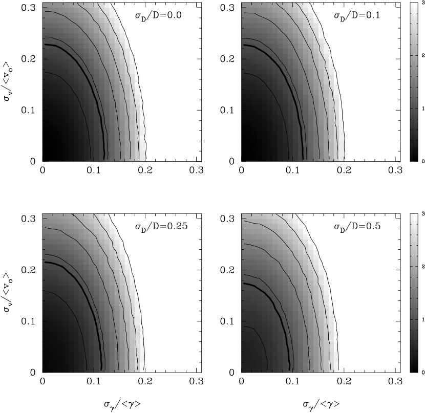
Figure 2: Images of ${\sigma}^{2}$ from the size-line width fits for an ensemble of clouds with varying turbulent properties parameterized by $\sigma_{v}$/$<v_{\circ}>$ and $\sigma_{\gamma}$/$<\gamma>$ for different distances uncertainties ($\sigma_{D}/D$=0,0.1,0.25, and 0.5). The light contour values of ${\sigma}^{2}$ are 0.5, 1.0, 1.5 2, 2.5, 3.0 $km^{2}s^{-2}$. The heavy contour in each plot shows the loci that correspond to $\sigma_{obs}^{2}$=0.88 km² s^-2 from Solomon et al. (1987) and provides an observational upper limit to cloud-to-cloud variations of $v_{\circ}$ and $\gamma$. These loci demonstrate that the structure function parameters, $\gamma$ and $v_{\circ}$, can not vary by more than $\sim$10-20%.

The Monte Carlo results are shown in Figure 2 where $\sigma_{v}$ and $\sigma_{\gamma}$ are normalized by $<v_{\circ}>$ and $<\gamma>$ respectively to reflect the fractional variation. The heavy solid line shows the value of ${\sigma}_{obs}^{2}$=0.88 $km^{2}s^{-2}$ from the Solomon et al. (1987) sample. This contour defines the locus of $\sigma_{v}/<v_{\circ}>$, $\sigma_{\gamma}/<\gamma>$ points that reproduce the observed scatter in the Solomon et al. (1987) size-line width relationship. In the unlikely extreme limit that $\sigma_{\gamma}$=0, then the most $\sigma_{v}$ can vary is 18-23% about the observed value of 0.9 km s^-1. Conversely, if $\sigma_{v}$=0, then $\sigma_{\gamma}$ can vary by less than 9-12% about its fiducial value of 0.5. More realistically, $\sigma_{v}\neq 0$ and $\sigma_{\gamma}\neq 0$, so the percent variations for both parameters are $\sim$8-12%. We emphasize that these are upper limits to the true variations between clouds as $\sigma_{v}$ and $\sigma_{\gamma}$ also include measurement errors and biased mapping effects that are likely present in all cloud-to-cloud size-line width relationships.

4 Implications of Invariant Interstellar Turbulence

The upper limits to variations of the structure function parameters are quite small when one considers the large range of molecular cloud environments. With few exceptions, giant molecular clouds are sites of massive star formation. The massive stars can, in principle, affect gas dynamics over the extent of a cloud by enhancing the UV radiation field, driving HII region expansions and stellar winds, and are the progenitors of supernova explosions. The star formation activity in smaller clouds is generally limited to the birth of low mass stars whose impact on cloud dynamics by protostellar winds is highly localized and small with respect to the integrated energy input from massive stars. For the sample of molecular clouds used in this study, the far infrared IRAS point source luminosities range from 20 $L_{\odot}$  (B18, Heiles’ Cloud 2, L1228) to 7.6$\times$10⁵ $L_{\odot}$  (NGC 7538). Despite the large differences in the amount of internal energy injection from newborn stars, the functional forms of the turbulent structure functions for all clouds are similar. Either all clouds coincidentally redistribute this internal energy into turbulent, random motions described by structure functions with the same slopes and amplitudes via some self-regulatory process or these internal energy sources are small compared to an external energy reservoir that is common to all regions in the Galaxy. Brunt et al. (2004) show that most of the turbulent energy of a molecular cloud resides on the largest scales and that the cloud dynamics are more readily accounted by large scale driving of turbulence. The universality of turbulence described in this study provides additional evidence for large scale driving sources within the molecular interstellar medium. The narrow range of turbulent flow parameters may also reflect the necessary conditions that facilitate the development of molecular clouds. Regions with extreme, high values of $v_{\circ}$ may be highly overpressured with respect to self-gravity and expand to larger, more diffuse configurations with less effective self-shielding to sustain significant molecular abundances.

Larson (1981) presaged the results from recent numerical simulations that molecular clouds are short lived ($<$10⁷ years), transient objects (Ballesteros-Paredes, Hartmann, & Vazquez-Semadeni 1999) that must be continually reassembled from the diffuse gas component. His suggestion that molecular clouds result from thermal instabilities within shocks of colliding atomic gas streams is similar to recent numerical simulations of compressible turbulence that show the development of high density regions directly from the shocks (Hunter et al. 1986; Elmegreen 1993; Ballesteros-Paredes, Vazquez-Semadeni, & Scalo 1999). Such a common dynamical origin of molecular clouds in the Galaxy may account for the measured near invariance of turbulence.

The results presented in this study apply to the low density gas substrate that comprises most of the mass and volume of a molecular cloud. Turbulent properties may indeed differ between clouds within the high density, localized, supercritical core regions. In distributed, low mass star forming regions, the non-thermal motions within the dense gas are subsonic (Benson & Myers 1989). Within the massive cores typical of clustered star forming regions, the observed velocities are supersonic (Pirogov et al. 2003). The identification of processes responsible for such divergent, dense gas configurations remains one of the primary challenges to descriptions of star formation (Klessen, Heitsch, & Mac Low 2000; Padoan & Nordlund 2002; Vazguez-Semadeni, Ballesteros-Paredes, & Klessen 2003; Shu et al. 2004; Mac Low & Klessen 2004).

5 Summary

We have examined the degree to which interstellar turbulence is universal within the molecular gas component of the Galaxy by comparing the measured structure functions for 27 giant molecular clouds. Despite the large differences in cloud environments and local star formation activity, the structure functions are described by very narrow ranges of the scaling exponent and scaling coefficient. The degree of universality is further constrained by Monte Carlo simulations that replicate the observed scatter in the Larson scaling law that describes the relationship between global velocity dispersion and cloud size. The near invariance of turbulence within the molecular interstellar medium suggests a common formation mechanism of molecular clouds such as shocks due to colliding gas streams of diffuse, atomic material as originally suggested by Larson (1981). It also implies that the energy contribution from internal sources such as stellar winds and expanding HII regions may be small with respect to a common, external component.

Figure 1: The composite ${\delta}v,l$ relationship from PCA decompositions of ¹²CO J=1-0 imaging observations of 27 individual molecular clouds. The small scatter of points attest to the near invariance of interstellar turbulence within molecular clouds that exhibit a large range in size, environment, and star formation activity. The large filled circles are the global velocity dispersion and size for each cloud derived from the first principal component. These are equivalent to the global velocity dispersion and size of the cloud as would be measured in the cloud-to-cloud size-line width relationship (Larson 1981; Solomon et al. 1987). The light solid line show the bisector fit to all points from all clouds. The heavy solid line shows the bisector fit to the filled circles exclusively. The similarity of these two power laws explains the connection of Larson’s cloud-to-cloud scaling law to the structure functions of individual clouds.

References

- Ballesteros-Paredes, Vazquez-Semadeni, & Scalo (1999) Ballesteros-Paredes, J.E., Vazquez-Semadeni, E., & Scalo, J. 1999, ApJ, 514, 286
- Ballesteros et al. (1999) Ballesteros-Paredes, J.E., Hartmann, L., & Vazquez-Semadeni, E. 1999, ApJ, 527, 285
- (3) Ballesteros-Paredes, J.E. & Mac Low, M. 2002, ApJ, 570, 734
- Benson & Myers (1989) Benson, P.J. & Myers, P.C. 1989, ApJS, 71, 89
- Brunt & Heyer (2002) Brunt, C.M. & Heyer, M.H. 2002, ApJ, 566, 276
- Brunt (2003) Brunt, C.M. 2003, ApJ, 584, 293
- Brunt et al. (2003) Brunt, C.M., Heyer, M.H., Vazquez-Semadeni, E., & Pichardo, B. 2003, ApJ, 595, 824
- Brunt & Mac Low (2004) Brunt, C.M. & Mac Low, M. 2004, ApJ, 604, 196
- Brunt et al. (2004) Brunt, C.M., Heyer, M.H., Zivkov, V., & Mac Low, M. 2004, ApJ, in press
- Carr (1987) Carr, J.S. 1987, ApJ, 323, 170
- Elmegreen (1993) Elmegreen, B.G. 1993, ApJ, 419, L29
- Falgarone et al. (1992) Falgarone, E. Puget, J.-L., Pereault, M. 1992, A&A, 257, 715
- Fuller & Myers (1992) Fuller, G.A. & Myers, P.C. 1992, ApJ, 384, 523
- Heyer & Schloerb (1997) Heyer, M.H. & Schloerb, F.P. 1997, ApJ, 475, 173
- Heyer et al. (1998) Heyer, M.H., Brunt, C., Snell, R.L., Howe, J.E., Schloerb, F.P., & Carpenter, J.M. 1998, ApJS, 115, 241
- Hunter et al. (1986) Hunter, J.H., Sandford, M.T., Whitaker, R.W., & Klein, R.I. 1986, ApJ, 305, 309
- Larson (1981) Larson, R.B. 1981, MNRAS, 194, 809
- Loren (1989) Loren, R.B., 1989, ApJ, 338, 925
- Klessen et al. (2000) Klessen, R.S., Heitsch, F., & Mac Low, M. 2000, ApJ, 535, 887
- Mac Low & Klessen (2004) Mac Low, M., & Klessen, R.S. 2004, Reviews of Modern Physics, 76, 125
- Padoan & Nordlund (2002) Padoan, P. & Nordlund, A. 2002, ApJ, 576, 870
- Pirogov etal (2003) Pirogov, L., Zinchenko, I., Caselli, P., Johansson, L.E.B., & Myers, P.C. 2003, A&A, 405, 639
- Shu et al. (2004) Shu, F.H., Li, Z-Y, & Allen, A. 2004, ApJ, 601, 930
- Simon et al. (2001) Simon, R., Jackson, J.M., Clemens, D.P., Bania, T.M., & Heyer, M.H. 2001, ApJ, 551, 747
- Solomon et al. (1987) Solomon, P.M., Rivolo, A.R., Barrett, J., & Yahil, A. 1987, ApJ, 319, 730
- Stutzki & Gusten (1990) Stützki, J. & Güsten, R. 1990, ApJ, 356, 513
- Vazquez et al. (2003) Vazquez, E., Ballesteros-Paredes, J.E. & Klessen, R.S. 2003, ApJ, 585, L131