Presupernova Evolution of Differentially Rotating
Massive Stars Including Magnetic Fields

Abstract

As a massive star evolves through multiple stages of nuclear burning on its way to becoming a supernova, a complex, differentially rotating structure is set up. Angular momentum is transported by a variety of classic instabilities, and also by magnetic torques from fields generated by the differential rotation. We present the first stellar evolution calculations to follow the evolution of rotating massive stars including, at least approximately, all these effects, magnetic and non-magnetic, from the zero-age main sequence until the onset of iron-core collapse. The evolution and action of the magnetic fields is as described by Spruit (2002) and a range of uncertain parameters is explored. In general, we find that magnetic torques decrease the final rotation rate of the collapsing iron core by about a factor of 30 to 50 when compared with the non-magnetic counterparts. Angular momentum in that part of the presupernova star destined to become a neutron star is an increasing function of main sequence mass. That is, pulsars derived from more massive stars will rotate faster and rotation will play a more dominant role in the star’s explosion. The final angular momentum of the core is determined - to within a factor of two - by the time the star ignites carbon burning. For the lighter stars studied, around $15\,{\mathrm{M}_{\odot}}$, we predict pulsar periods at birth near $15\,{\mathrm{ms}}$, though a factor of two range is easily tolerated by the uncertainties. Several mechanisms for additional braking in a young neutron star, especially by fall back, are also explored.

1 Introduction

Massive stars are known to be rapid rotators with typical equatorial velocities around 200 ${\mathrm{km}}\,{\mathrm{s}}^{-1}$ or more during hydrogen burning (Fukuda, 1982). It has long been known that this much rotation could have a significant influence on the evolution of the star, both on the main sequence and during in its later stages of evolution (e.g., Endal & Sophia, 1976; Endal & Sofia, 1978; Heger et al., 2000; Maeder & Meynet, 2001; Hirishi et al., 2004). For example, on the main sequence, surface abundance patterns are observed (e.g., Gies & Lambert, 1992; Herrero, 1994; Vrancken et al., 2000; Venn, 1999) that are most naturally explained by rotationally-induced mixing in the stellar interior (e.g., Venn, 1999; Heger & Langer, 2000; Meynet & Maeder, 2000).

Numerical studies of of the later evolutionary stages of rotating massive stars initially found that the stellar core would reach critical (Keplerian) rotation by the time carbon ignited in the core (e.g., Kippenhahn et al., 1970; Endal & Sophia, 1976), especially when angular momentum transport is neglected. Thus one might encounter triaxial deformation early on, with continued evolution hovering near instability. Modern stellar models that include more instabilities capable of transporting angular momentum find that considerable angular momentum is lost from the core during hydrogen and helium burning (Endal & Sofia, 1978), especially when the stabilizing effect of composition gradients is reduced (Pinsonneault et al., 1989; Heger et al., 2000; Maeder & Meynet, 2001; Hirishi et al., 2004). Such stars now evolve to iron core collapse, but still form very rapidly rotating ($\sim 1\,{\mathrm{ms}}$) neutron stars.

However, with the exception of Spruit & Phinney (1998) and Maeder & Meynet (2004), all studies of massive stellar evolution to date have ignored what is probably a major effect, the torques exerted in differentially rotating regions by the magnetic fields that thread them. This omission has not been because such torques were thought to be unimportant, but because of the complexity and uncertainty of carrying out even one-dimensional calculations that included them. This uncertainty, in turn, related to the absence of a credible physical theory that would even qualitatively describe the separate evolution of the radial and poloidal components of the field, both of which are necessary to calculate the torque,

$$S=\frac{B_{r}B_{\phi}}{4\pi}$$ (1)

Spruit & Phinney (1998) estimated these torques assuming that the poloidal field results from differential winding and that the radial field would, due to the action of unspecified instabilities, be comparable. Particular attention was paid to the region of large shear that separates the core of helium and heavy elements from the very slowly rotating hydrogen envelope of a red supergiant star. This assumption, ${B_{r}}\sim{B_{\phi}}$, probably overestimated the actual ${B_{r}}$ by orders of magnitude and the rotation rates that Spruit & Phinney (1998) estimated for young pulsars were thus too slow (see also Livio & Pringle 1998).

More recently, Spruit (2002) has provided improved estimates for ${B_{r}}$ and ${B_{\phi}}$ based upon a dynamo process that takes into account the effect of stable stratifications. Here we investigate the effect of this prescription in a stellar evolution code used to study the complete evolution of massive stars. Particular attention is given to the rotation rate it implies for young neutron stars. In §2, we describe the physical and numerical modeling. In §3, the results for $12$, $15$, $20$, $25$ and $35\,{\mathrm{M}_{\odot}}$ stars are presented and, in §4, compared with observational data. Typical neutron star rotation rates, at birth, are $\sim$ $15\,{\mathrm{ms}}$. In §5 we discuss other possible ways that such rapidly rotating stars might be slowed during the first days of their evolution by magnetic winds and fall back. The surface abundance changes due to rotationally-induced mixing are discussed in §6 and in §7 we give our conclusions.

2 Implementation of Magnetic Braking

The treatment of magnetic torques given by Spruit (2002) was implemented in a version of the implicit hydrodynamics stellar evolution code (KEPLER, Weaver et al., 1978) that already included angular momentum transport and mixing due to a number of non-magnetic processes. See Heger et al. (2000) for a discussion of these non-magnetic instabilities and Spruit (1999, 2002) for a detailed description of the dynamo mechanism. Here we discuss only the implementation of and results from that physical model.

Both angular momentum transport and chemical mixing are calculated by solving the time-dependent diffusion equation (Heger et al., 2000). It is assumed that the dynamo adjusts and reaches equilibrium field strength on a time-scale that is short compared to the evolution time-scales of the star, i.e., we neglect the time required to reach the steady state field strength and distribution described by Spruit (2002) and only apply their equilibrium values. This should be a reasonable approximation in all but the most advanced burning stages that occur when the angular momentum distribution has already been frozen in. The validity of this assumption is revisited in §7

2.1 The dynamo process in radiative regions

Spruit (2002) discusses two limiting cases: stabilization by composition gradients (Spruit’s Case 0), and stabilization by superadiabatic temperature gradients (Spruit’s Case 1). Realistic stellar models exhibit both kinds of gradients at same time, so the intermediate case must also be included (see also Maeder & Meynet 2004).

The effective viscosity, ${\nu_{\mathrm{e}}}$, for the radial transport of angular momentum results from azimuthal stress due to the field generated by the dynamo, $S={B_{r}}{B_{\phi}}/4\pi$. Its value is given by

$${\nu_{\mathrm{e}}}\equiv S/\rho q\Omega\;.{}$$ (2)

See also eqs. 34-40 of Spruit (2002). We also implement the “effective diffusivity”, ${D_{\mathrm{e}}}\equiv{\eta_{\mathrm{e}}}$, given in his eqs. 41-43. Here $\Omega$ is the angular velocity, $q=\mathrm{d}\ln\Omega/\mathrm{d}\ln r$ is the shear, $r$ is the radius, $\rho$ is the density, and $S$ is the stress.

For application outside the regime of “ideal gas with radiation” where the gradient of the mean molecular weight determines the stabilization, we replace $N^{2}_{\mu}$ by a more general formulation (“$N^{2}_{\mathrm{\!comp}}$”), but do not change nomenclature. This way the discussion in Spruit (2002) can be followed without further revision. Generally, the Bruntväsälä frequency is

$${N^{2}}=\frac{g}{{H_{\mathrm{P}}}}\left(\frac{1}{{\Gamma\!_{1}}}-\frac{\mathrm{d}\ln\rho}{\mathrm{d}\ln P}\right)\;,$$ (3)

where $g=-GM(r)/r^{2}$ is the local gravitational acceleration, $P$ is the pressure, ${H_{\mathrm{P}}}=-\mathrm{d}r/\mathrm{d}\ln P$ is the pressure scale height, and the derivatives are total derivatives in the star. The compositional contribution to the Bruntväsälä frequency is given by

$${N^{2}_{\mu}}=\frac{g}{{H_{\mathrm{P}}}}\left(\alpha-\delta\frac{\mathrm{d}\ln T}{\mathrm{d}\ln P}-\frac{\mathrm{d}\ln\rho}{\mathrm{d}\ln P}\right)\;,$$ (4)

where $T$ is the temperature. The thermodynamic quantities $\alpha$, $\delta$, and ${\Gamma\!_{1}}$ obey their common definitions (e.g., Kippenhahn & Weigert 1990). Again, the derivatives are the actual gradients in the star, not thermodynamic derivatives. The thermal contribution to the Bruntväsälä frequency is then given by

$${N^{2}_{T}}={N^{2}}-{N^{2}_{\mu}}=\frac{g}{{H_{\mathrm{P}}}}\left(\frac{1}{{\Gamma\!_{1}}}-\alpha+\delta\frac{\mathrm{d}\ln T}{\mathrm{d}\ln P}\right)\;.$$ (5)

As stated above, we use the symbol ${N^{2}_{\mu}}$ to indicate (the square of) the Bruntväsälä frequency due to the composition gradient for a general equation of state ($\equiv{N^{2}_{\mathrm{comp}}}$), not just due to changes of mean molecular weight, $\mu$. Appendices A and B give a derivation of the general expressions. This formulation is identical with the stability analysis for the different regimes (next section) as used in KEPLER, and therefore necessary for consistency in regimes where the assumption of an ideal gas is a poor approximation.

2.2 The dynamo in semiconvective and thermohaline regions

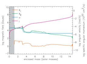
Figure 1: Magnetic field structure and angular momentum distribution for the standard $15\,{\mathrm{M}_{\odot}}$ model at at hydrogen depletion (upper left), helium ignition (upper right), helium depletion (lower left), and carbon ignition (lower right). See Table 1 for the definitions of these times. The shaded regions are those portions of the star that are convective. In those regions large diffusion coefficients for angular momentum lead to nearly rigid rotation in all but the latest stages of the evolution.

In addition to the radiative regime, I, where both composition gradients and temperature gradients are stabilizing, other regimes have to be considered in which “secular” mixing processes operate. These are secular as opposed to processes like convection that operate on a hydrodynamic time scale. Two of these are semiconvection (II; where a stabilizing composition gradient dominates a destabilizing temperature gradient) and thermohaline convection, also called the salt-finger instability (III; where a stabilizing temperature gradient dominates a destabilizing composition gradient; e.g., Braun, 1997; Heger et al., 2000, their Figure 1 for an overview). The final regime of hydrodynamic instability in non-rotating stars is that of Ledoux convection (Ledoux 1958; Regime IV; wehere the destabilizing temperature gradient is stronger than any stabilization by the composition gradient). In the Ledoux regime, effective viscosities and diffusivities are given by mixing length theory (Heger et al., 2000). A very approximate treatment of Regimes II and III is given in the next two sections.

2.2.1 The semiconvective case

In semiconvective regions (Regime II), the square of the thermal buoyancy frequency is negative and thus the limiting Case 1 would be convection. Instead of equation (34) of Spruit (2002), we first compute an “dynamo” effective viscosity by

$${\nu_{\mathrm{re}}}={\nu_{\mathrm{e0}}}f(q)\;,$$ (6)

with $\nu_{\mathrm{e0}}$ from equation (35) of Spruit (2002) and ${q_{\mathrm{min}}}={q_{0}}$ (equations 37-39 of Spruit 2002).

Adopting a model for semiconvection in the non-linear regime similar to Spruit (1992), we assume the radiative flux is transported by convective motions in the semiconvective layers. For the sake of simplicity, we compute an effective turbulent viscosity, $\nu_{\mathrm{sc}}$, from the velocities according to mixing-length theory (Schwarzschild & Härm, 1958) assuming Schwarzschild convection (i.e., when the $\mu$ gradient is neglected),

$${v_{\mathrm{conv}}}\equiv\left(\frac{g\delta{H_{\mathrm{P}}}L}{64\pi\rho{c_{\mathrm{P}}}Tr^{2}}\right)^{\!1/3}$$ (7)

(e.g., as derived from equations 7.6 and 7.7 of Kippenhahn & Weigert, 1990) and an assumed characteristic length scale of $H_{\mathrm{P}}$ by

$${\nu_{\mathrm{sc}}}\equiv\frac{1}{3}{H_{\mathrm{P}}}{v_{\mathrm{conv}}},$$ (8)

(however, see Spruit, 1992), and $c_{\mathrm{P}}$ is the specific heat capacity at constant pressure.

Finally, we assume that the actual viscosity is somewhere between that of the case of mere semiconvection and that of the dynamo dominated by composition stratification and take the geometric mean between the two viscosities,

$${\nu_{\mathrm{e}}}\equiv\sqrt{{\nu_{\mathrm{re}}}{\nu_{\mathrm{sc}}}}\;{}.$$ (9)

The effective turbulent diffusion coefficient, ${D_{\mathrm{e}}}$, is computed in an analogous way, $\nu_{\mathrm{re}}$, i.e., ${D_{\mathrm{e}}}={D_{\mathrm{e0}}}f(q)$, ${q_{\mathrm{min}}}={q_{0}}$. Due to the properties of the layers semiconvection model (Spruit, 1992) – negligible diffusivity in typical stellar environments –, we do not compute a geometric mean with the semiconvective diffusivity similar to Eq. (9). Instead we just add it to the semiconvective diffusion coefficient computed in KEPLER. Typically it is negligible.

2.2.2 The thermohaline case

In this regime (III) the compositional buoyancy frequency becomes negative and the limiting Case 0 would be Rayleigh-Taylor unstable. We assume the limiting Case 1 of Spruit (2002) and compute ${\nu_{\mathrm{e}}}={\nu_{\mathrm{e1}}}$, ${D_{\mathrm{e}}}={D_{\mathrm{e1}}}$, and ${q_{\mathrm{min}}}={q_{1}}$, analogous to the semiconvective case.

In massive stars, thermohaline convection typically occurs following radiative shell burning in the fuel “trace” left behind by an receding central convective burning phase. The higher temperature of shell burning can sometimes create heavier ashes than core burning and the resulting compositional structure is unstable. The contraction phase after central helium burning is the most important domain in massive stars.

Generally, the motions associated with the growth of this instability (“salt fingers”) are very slow. Thus the interaction with the dynamo is much more restricted than in the case of semiconvection. Therefore we do not employ a interpolation between the dynamo effective radial viscosity or diffusivity as is done in §2.2.1.

2.3 Evaluating the magnetic field strength

The most interstesting result of the dynamo model is the magnetic field strength. Combining equations (21), (23), (35) and (36) of Spruit (2002), one has

$${\nu_{\mathrm{e}}}=r^{2}\Omega\left(\frac{{B_{r}}}{{B_{\phi}}}\right)^{\!2}\;.$$ (10)

Using his equation (28), the components of the field are:

$${B_{r}^{4}}=16\pi^{2}\rho^{2}{\nu_{\mathrm{e}}}^{3}q^{2}\Omega r^{-2}$$ (11)

$${B_{\phi}^{4}}=16\pi^{2}\rho^{2}{\nu_{\mathrm{e}}}q^{2}\Omega^{3}r^{2}\;.$$ (12)

3 Results Including Magnetic Torques

3.1 Implementation

Based upon the assumptions in §2, the full evolution of stars of $12$, $15$, $20$, $25$, and $35\,{\mathrm{M}_{\odot}}$ of solar metallicity was calculated. For comparison, equivalent models were also calculated without magnetic fields for three of these stars. The initial models and input physics were the same as in Rauscher et al. (2001), but the total angular momentum of the star was chsen such that a typical initial equatorial rotation velocity of $\sim 200\,{{\mathrm{km}}\,{\mathrm{s}}^{-1}}$ (Fukuda, 1982) was reached on the zero-age main sequence (ZAMS; see Heger et al. 2000). Time-dependent mixing and angular momentum transport were followed as discussed by Heger et al. (2000) with the turbulent viscosities and diffusivities from the dynamo model added to those from the model for the hydrodynamic instabilities. For the time being, possible interactions between the two are neglected (though see Maeder & Meynet 2004). Our standard case (B) implements the description as outlined in the previous sections.

3.2 Presupernova Models and Pulsar Rotation Rates

Tables 1 - 6 and Fig. 1 summarize our principal results. As also noted by Maeder & Meynet (2004), the inclusion of magnetic torques with a magnitude given by Spruit (2002), greatly decreases the differential rotation of the star leading to more slowly rotating cores.

For illustration, we consider in some detail the evolution of the $15\,{\mathrm{M}_{\odot}}$ model with standard parameter settings. Table 1 shows that, over the course of the entire evolution, the total angular momentum enclosed by fiducial spheres of mass coordinate $1.5$, $2.5$, and $3.5\,{\mathrm{M}_{\odot}}$ decreases in the magnetic models by a factor of 100 to 200, far more than in the non-magnetic comparison model. In both cases most of the angular momentum transport occurs prior to carbon ignition (Figs. 2 and 3). The greatest fractional decrease occurs during the transition from hydrogen depletion to helium ignition (Table 1, Fig. 2) as the star adjusts to its new red giant structure. During this transition, the central density goes up by a factor of about 100 (from $11\,{{\mathrm{g}}\,{\mathrm{cm}}^{-3}}$ to $1400\,{{\mathrm{g}}\,{\mathrm{cm}}^{-3}}$) with an accompanying increase in differential rotation and shear. Though the angular momentum evolves little after carbon burning, modified only by local shells of convection, there is a factor of two change after carbon ignition (central temperature = $5{\times{10^{8}}}\,{\mathrm{K}}$).

The magnetic torques are sufficiently strong to enforce rigid rotation both on the main sequence and in the helium core during helium burning for all masses considered (see also Maeder & Meynet 2004). The appreciable braking that occurs during hydrogen and helium burning is therefore a consequence of mass loss and evolving stellar structure, especially the formation of a slowly rotating hydrogen envelope around a rapidly rotating helium core. Typically the more massive stars spend a shorter time during the critical Kelvin-Helmholtz contraction between hydrogen depletion and helium ignition and also have a shorter helium burning lifetime. Hence, even though they actually have a little less angular momentum at the fiducial mass points in Table 1 on the main sequence, the more massive stars have more angular momentum in their cores at the end of helium burning. This distinction persists and the more massive stars give birth to more rapidly rotating neutron stars.

Stars that include all the usual non-magnetic mechanisms for rotational mixing and angular momentum transport (Heger et al., 2000), but which lack magnetic fields have a considerably different evolution and end up with 30 to 50 times more angular momentum in that part of their core destined to collapse to a neutron star (Tables 1 and 3, Figs. 2 and 3). Most notable is the lack of appreciable braking of the helium core by the outer layers in the period between hydrogen core depletion and helium ignition. The post-carbon-ignition braking that accounted for an additional factor of two in the magnetic case is also much weaker. In fact, the inner $1.5\,{\mathrm{M}_{\odot}}$ of the $15\,{\mathrm{M}_{\odot}}$ model has only about five times less angular momentum at core collapse than implied by strict conservation from the (rigidly rotating) main sequence onwards. As noted previously many times, such a large amount of angular momentum would have important consequences for the supernova explosion mechanism. Rigidly rotating neutron stars cannot have a period shorter than about $1\,{\mathrm{ms}}$.

Table 2 gives the magnetic field components that exist in different parts of the star during different evolutionary phases. The magnetic field is highly variable from location to location in the star and the values given are representative, but not accurate to better than a factor of a few (Fig. 1), especially during the late stages. As expected, the toroidal field, which comes from differential winding is orders of magnitude larger than the radial field generated by the Tayler instability. The product ${B_{\phi}}{B_{r}}$ scales very approximately as the central density with the ratio ${{B_{r}}/{B_{\phi}}}\sim{10^{-3}}-{10^{-4}}$. Though the formulae used here are expected to break down during core collapse, a simple extrapolation to ${10^{15}}\,{{\mathrm{g}}\,{\mathrm{cm}}^{-3}}$ for the central density of a neutron star suggests ${B_{\phi}}\sim{10^{14}}$ and ${B_{r}}\sim{10^{10}}$.

Table 3 gives the expected pulsar rotation rates based upon a set of standard assumptions. Following Lattimer & Prakash (2001), it is assumed that all neutron stars (with realistic masses) have a radius of $12\,{\mathrm{km}}$ and a moment of inertia $0.35\,M_{\mathrm{grav}}R^{2}$. Adding the binding energy to the gravitational mass, assumed in Table 3 to be $1.4\,{\mathrm{M}_{\odot}}$ gives the baryonic mass of the core that collapsed to the neutron star, $1.7\,{\mathrm{M}_{\odot}}$. Taking the angular momentum inside $1.7\,{\mathrm{M}_{\odot}}$ from the presupernova model, assuming conservation during collapse, and solving for the period then gives the values in the table.

3.3 Sensitivity To Uncertain Parameters

It is expected that our results will be sensitive to several uncertain factors including the effect of composition gradients, the efficiency of the dynamo in generating magnetic field, and the initial angular momentum of the star. To some extent, these uncertainties are ameliorated by the strong sensitivity of the expected magnetic torques to rotation speed and differential shear (eq. 34–36 of Spruit 2002). Composition gradients have very significant influence on the resulting angular momentum transport by inhibiting the action of the dynamo. In particular, composition interfaces, as resulting from the nuclear burning processes in combination with convection, usually also show significant shear, but if the dynamo action is suppressed by a steep change in mean molecular weight, angular momentum can become “trapped” in a fashion similar to that observed by Heger et al. (2000). To illustrate the uncertainties of the dynamo model, we studied several test cases where the stabilizing effect of composition gradients is varied by multiplying $N^{2}_{\mu}$ and $N^{2}_{T}$ by 1/10. We also explored multiplying the overall coefficient of the torque in eq. (1) by varying ${B_{\phi}}{B_{r}}$ by a factor of ten and multiplied the initial rotational rate by 0.5 and 1.5 (Table 3).

In three cases, the $20$ and $25\,{\mathrm{M}_{\odot}}$ with high rotation rate, and the “normal” $35\,{\mathrm{M}_{\odot}}$ model, the star lost its hydrogen-rich envelope due to mass loss either during ($25$ and $35\,{\mathrm{M}_{\odot}}$) or just at the end ($20\,{\mathrm{M}_{\odot}}$) of it evolution. The KEPLER code was not able to smoothly run these models through the period where they lost their last solar mass of envelope because violent pulsations were encountered. The last 0.5 to $1.0\,{\mathrm{M}_{\odot}}$ was thus removed abruptly and the calculation continued for the resulting Wolf-Rayet star. However, it is clear that removing the envelope removes an appreciable braking torque on the helium core so it is reasonable that the remnants of such stars rotate more rapidly.

3.4 Variable Neutron Star Masses

Since the iron core masses, silicon shell masses, and density profiles all differ appreciably for presupernova stars in the 12 to $35\,{\mathrm{M}_{\odot}}$ range, it is not realistic to assume that they all make neutron stars of the same mass. Ideally, one would extract realistic masses from a reliable, credible model for the explosion, but, unfortunately, such models have not reached the point of making accurate predictions. Still there are some general features of existing models that provide some guidance. As noted by Weaver et al. (1978), the remnant mass cannot typically be less than the mass of the neutronized iron core. Otherwise one overproduces rare neutron-rich isotopes of the iron group. More important to the present discussion, successful explosions, when they occur in modern codes, typically give “mass cuts” in the vicinity of large entropy jumps. The reason is that a jump in the entropy corresponds to sudden decrease in the density. This in turn implies a sudden fall off in accretion as the explosion develops. The lower density material is also more loosely bound by gravity. The largest jump in the vicinity of the iron core is typically at the base of the oxygen burning shell and that has sometimes been used to estimate neutron star masses (Timmes et al., 1996). Recent studies by Thomas Janka (private communication) suggest a numerical criterion, that the mass cut occurs where the entropy per baryon equals $4\,{k_{\mathrm{B}}}$. In Table 4, instead of assuming a constant baryonic mass of $1.7\,{\mathrm{M}_{\odot}}$ for the neutron star progenitor (as in Table 3), we take the value where the specific entropy is $4\,{{k_{\mathrm{B}}}/\mathrm{baryon}}$.

As expected this prescription gives larger baryonic masses for the remnant (“Baryon” in the table). The fraction of this mass that is carried away by neutrinos is given by Lattimer & Prakash (2001),

$$f=\frac{0.6\beta}{1-0.5\beta}$$ (13)

where $\beta=GM_{\mathrm{grav}}/Rc^{2}$. When this is subtracted, one obtains the gravitational masses, $M_{\mathrm{grav}}$ in Table 4. Using these, assuming once more a moment of inertia $I=0.35M_{\mathrm{grav}}R^{2}$ and a radius of $12\,{\mathrm{km}}$, and conserving angular momentum in the collapse one obtains the period. Because the angular momentum per unit mass increases as one goes out in the star, using a larger mass for the remnant increases its rotation rate.

The resulting values are similar to those in Table 3 for the same “standard” parameter settings, but show even more clearly the tendency of larger stars to make more rapidly rotating pulsars. They also show an additional prediction of the model - that more massive pulsars will rotate more rapidly. The numbers in Table 4 have not been corrected for the fact that the typical neutrino, since it last interacts at the edge of the neutron star, carries away more angular momentum than the average for its equivalent mass. Thus the periods in Table 4 can probably be multiplied by an additional factor of $\sim 1.2$ (Janka, 2004).

4 Comparison With Observed Pulsar Rotation Rates

Table 5 gives the measured and estimated rotation rates and angular momenta of several young pulsars at birth (Muslimov & Page, 1996; Marshall el al., 1998; Kaspi et al., 1994). To estimate the angular momenta in the table, we have assumed, following Lattimer & Prakash (2001), that the moment of inertia for ordinary neutron stars (not quark stars) is $I\approx 0.35MR^{2}\approx 1.4{\times{10^{45}}}\,{{\mathrm{g}}\,{\mathrm{cm}}^{2}}$. Here a constant fiducial gravitational mass of $1.4\,{\mathrm{M}_{\odot}}$ is assumed.

Given the uncertainties in both our model and the extrapolation of observed pulsar properties, the agreement, at least for the 12 - $15\,{\mathrm{M}_{\odot}}$ models, is quite encouraging. This true all the more so when one realizes that the periods in Tables 3 and 4 should be multiplied by a factor of approximately $1.2-1.3$ to account for the angular momentum carried away by neutrinos when the neutron star forms (Janka, 2004). Then our standard, numerically typical supernova, $15\,{\mathrm{M}_{\odot}}$, would produce a neutron star with angular momentum $5.8{\times{10^{47}}}\,{{\mathrm{erg}}\,{\mathrm{s}}}$ (“PreSN” entry in Table 1 divided by 1.3). It should also be noted that the most common core collapse events - by number - will be in the $12$ to $20\,{\mathrm{M}_{\odot}}$ range because of the declining initial mass function. Moreover, stars above around $25$ - $30\,{\mathrm{M}_{\odot}}$ may end up making black holes (Fryer, 1999).

What then is the observational situation? Marshall el al. (1998) have discovered a pulsar in the Crab-like supernova remnant, N157B, in the Large Magellanic Cloud, with a rotation rate of $16\,{\mathrm{ms}}$. This is probably an upper bound to its rotation rate at birth. Glendenning (1996) gives an estimated initial rotation rate for the Crab pulsar itself of $19\,{\mathrm{ms}}$. Estimating the initial rotation rate of the much larger sample of pulsars, known to be rotating now much more slowly, is fraught with uncertainty. Nevertheless, PSR 0531+21 and PSR 1509-58 are also estimated to have been born with $\sim 20\,{\mathrm{ms}}$ periods Muslimov & Page (1996) (though 0540-69 is estimated to have $P_{0}\approx 39\,{\mathrm{ms}}$). At the other extreme, Pavlov et al. (2002) find for PKS1209-51/52 a rotation period of $424\,{\mathrm{ms}}$ and argue that the initial rate was not much greater. Similarly, Kramer et al. (2003) argue that the initial rotation rate of PSR J0538+2817 was $139\,{\mathrm{ms}}$.

5 Further Braking Immediately After the Explosion

5.1 r-Mode Instability

For some time it was thought that gravitational radiation induced by the “r-mode instability” would rapidly brake young neutron stars. However, Arras et al. (2003) found that the r-mode waves saturate at amplitudes lower than obtained in previous numerical calculations (Lindblom et al., 2001) that assumed an unrealistically large driving force. Much less gravitational radiation occurs and the braking time for a rapidly rotating neutron star becomes millennia rather than hours. Arras et al. calculate that

$$\tau_{\mathrm{s}pin\ down}=2000\ {\rm yr}\ (\frac{\alpha_{e}}{0.1})^{-1}\ (\frac{335\ {\rm Hz}}{\nu})^{11},$$ (14)

with $\alpha_{e}$, the maximum amplitude of the instability (for which Arras et al. estimate 0.1 as an upper bound). A $3\,{\mathrm{ms}}$ pulsar will thus take about 2000 years to substantially brake and the more slowly rotating neutron stars in Tables 3 and 4 will take even longer.

5.2 Neutrino-Powered Magnetic Stellar Winds

Woosley & Heger (2004) and Thompson et al. (2004) have discussed the possibility that a young, rapidly rotating neutron star will be braked by a magnetic stellar wind. This wind, powered by the neutrino emission of the supernova, may also be an important site for $r$-process nucleosynthesis (Thompson, 2003).

During the first $10\,{\mathrm{s}}$ of its life a neutron star emits about $20\,\%$ of its mass as neutrinos. This powerful flux of neutrinos passing through the proto-neutron star atmosphere drives mass loss and the neutron star loses $\sim 0.01\,{\mathrm{M}_{\odot}}$ (Duncan et al., 1986; Qian & Woosley, 1996; Thompson et al., 2001). Should magnetic fields enforce corotation on this wind out to a radius of 10 stellar radii, appreciable angular momentum could be lost from a $1.4\,{\mathrm{M}_{\odot}}$ neutron star (since $j\sim r^{2}\omega$). The issue is thus one of magnetic field strength and its radial variation.

For a neutron star of mass $M$ and radius, $R_{6}$, in units of $10\,{\mathrm{km}}$, the mass loss rate is approximately (more accurate expressions are given by Qian & Woosley)

$$\dot{M}\ \approx\ {10^{-3}}\ {\mathrm{M}_{\odot}}\ {\rm s^{-1}}\ \left(\frac{L_{\nu,{\rm tot}}}{{10^{53}}\ {{\mathrm{erg}}\,{\mathrm{s}}}}\right)^{5/3}\ {R_{6}}^{5/3}\ \left(\frac{1.4\,{\mathrm{M}_{\odot}}}{M}\right)^{2}.$$ (15)

The field will cause corotation of this wind out to a radius (Mestel & Spruit, 1987) where

$$\rho\ (v_{\mathrm{wind}}^{2}\ +\ \omega^{2}r^{2})\ \approx\ \frac{B^{2}}{4\pi}.$$ (16)

Calculations that include the effect of rotation on the neutrino-powered wind have yet to be done, but one can estimate the radial density variation from the one-dimensional models of Qian & Woosley (1996). For a mass loss rate of ${10^{-2}}\,{{\mathrm{M}_{\odot}}\,{\mathrm{s}}^{-1}}$ they find a density and radial speed at $100\,{\mathrm{km}}$ of ${10^{8}}\,{{\mathrm{g}}\,{\mathrm{cm}}^{-3}}$ and $1000\,{{\mathrm{km}}\,{\mathrm{s}}^{-1}}$ respectively. At this time, the proto-neutron star radius is $30\,{\mathrm{km}}$ and these conditions persist for $\sim 1\,{\mathrm{s}}$. Later, they find, for a mass loss rate of ${10^{-5}}\,{{\mathrm{M}_{\odot}}\,{\mathrm{s}}^{-1}}$ and a radius of $10\,{\mathrm{km}}$, a density at $100\,{\mathrm{km}}$ of $\sim{10^{5}}\,{{\mathrm{g}}\,{\mathrm{cm}}^{-3}}$ and velocity $2000\,{{\mathrm{km}}\,{\mathrm{s}}^{-1}}$. This lasts $\sim 10\,{\mathrm{s}}$. Unless $\omega$ is quite low, $v_{\mathrm{wind}}$ is not critical. For $\omega\sim 1000\,{\mathrm{rad}\,{\mathrm{s}}^{-1}}$ the field required to hold ${10^{8}}\,{{\mathrm{g}}\,{\mathrm{cm}}^{-3}}$ in corotation at $100\,{\mathrm{km}}$ is $\sim 3{\times{10^{14}}}\,{\mathrm{G}}$; for ${10^{5}}\,{{\mathrm{g}}\,{\mathrm{cm}}^{-3}}$ it is ${10^{13}}\,{\mathrm{G}}$.

To appreciably brake such a rapidly rotating neutron star, assuming $B\sim r^{-2}$, thus requires ordered surface fields of $\sim{10^{15}}$ - ${10^{16}}\,{\mathrm{G}}$. Similar conclusions have been reached independently by Thompson (2003). Such fields are characteristic of magnetars, but probably not of ordinary neutron stars. On the other hand if the rotation rate were already slow, $\omega\sim 100\,{\mathrm{rad}\,{\mathrm{s}}^{-1}}$ ($P\sim 60\,{\mathrm{ms}}$), even a moderate field of ${10^{14}}\,{\mathrm{G}}$ could have an appreciable effect. It should also be kept in mind that the field strength of a neutron star when it is $1$ - $10\,{\mathrm{s}}$ old could be very different than thousands of years later when most measurements have been made.

5.3 Fallback and the Propeller Mechanism

After the first $1000\,{\mathrm{s}}$, the rate of accretion from fall back is given (MacFadyen et al., 2001) by

$$\dot{M}\approx\ 10^{-7}\ t_{5}^{-5/3}\;{{\mathrm{M}_{\odot}}\,{\mathrm{s}}^{-1}},{}$$ (17)

with the time in units of ${10^{5}}\,{\mathrm{s}}$. For the mass loss rate in units of ${10^{26}}\,{{\mathrm{g}}\,{\mathrm{s}}^{-1}}$, we obtain

$$\dot{M}_{26}\ \approx\ 2\ t_{5}^{-5/3}\;{{\mathrm{g}}\,{\mathrm{s}}^{-1}}.{}$$ (18)

For a dipole field with magnetic moment $\mu_{30}=B_{12}{R_{6}}^{3}$, with $B_{12}$ the surface field in units of 10¹² G, the infalling matter will be halted by the field at the Alfven radius (Alpar, 2001),

$$r_{\!\!\mathrm{A}}\ =\ 6.8\ \mu_{30}^{4/7}\ \dot{M}_{26}^{-2/7}\ {\mathrm{km}}.{}$$ (19)

At that radius matter can be rotationally ejected, provided the angular velocity there corresponding to co-rotation exceeds the Keplerian orbital speed. The ejected matter carries away angular momentum and brakes the neutron star. This is the propeller mechanism (Illarionov & Sunyaev 1975; Chevalier 1989; Lin et al. 1991; Alpar 2001, but see the critical discussion in Rapport et al. 2004).

Obviously $r_{\!\!\mathrm{A}}$ must exceed the neutron star radius ($10\,{\mathrm{km}}$ here) if the field is to have any effect. The above equations thus require a strong field, $B>{10^{12}}\,{\mathrm{G}}$, and accretion rates characteristic of an age of at least one day. Additionally there is a critical accretion rate, for a given field strength and rotation rate, above which the co-rotation speed at the Alfven radius will be slower than the Keplerian orbit speed. In this case the matter will accrete rather than be ejected. Magnetic braking will thus be inefficient until $\omega^{2}\,r_{\!\!\mathrm{A}}^{3}\,>\,GM$, or

$$\dot{M}_{26}\ <\ 5.7{\times{10^{-4}}}\ \omega_{3}^{7/3}\ \mu_{30}^{2},{}$$ (20)

where $\omega_{3}$ is the angular velocity in thousands of radians per second ($\omega_{3}=1$ implies a period of $2\pi\,{\mathrm{ms}}$). This turns out to be a very restrictive condition. For a given $\mu_{30}$ and $\omega_{3}$, Eqs. (18) and (20) give a time, $t_{5,\mathrm{min}}$, when braking can begin. The torque on the neutron star from that point on will be

$$I\dot{\omega}\ =\ \mu^{2}/r_{\!\!\mathrm{A}}^{3}\ =10^{60}\frac{\mu_{30}^{2}}{r_{\!\!\mathrm{A}}^{3}},$$ (21)

with $I$, the moment of inertia of the neutron star, approximately ${10^{45}}$ (Lattimer & Prakash, 2001). The integrated deceleration will be

$$\Delta\omega\ =\ 250\,\mu_{30}^{2/7}\,t_{5,\mathrm{min}}^{-3/7}.$$ (22)

Putting it all together, a $1.4\,{\mathrm{M}_{\odot}}$ neutron star can be braked to a much slower speed ($\Delta\omega\sim\omega$) by fall back if $\mu_{30}>78$, $43$, or $25$ for initial periods of $6$, $21$, or $60\,{\mathrm{ms}}$, respectively. If the surface field strength - for a dipole configuration is less than $2{\times{10^{13\,}}}{\mathrm{G}}$, braking by the propeller mechanism will be negligible in most interesting situations.

However, we have so far ignored all non-magnetic forces save gravity and centrifugal force. A neutron star of age less than one day is in a very special situation. The accretion rate given by Eq. (17) is vastly super-Eddington. This means that matter at the Alfven radius will be braked by radiation as well as centrifugal force and the likelihood of its ejection is greater. Fryer et al. (1996) have considered neutron star accretion at the rates relevant here and find that neutrinos released very near the neutron star actually drive an explosion of the accreting matter. Just how this would all play out in a multi-dimensional calculation that includes magnetic braking, rotation, and a declining accretion rate has yet to be determined, but is worth some thought.

If the accreting matter is actually expelled under ‘propeller’ conditions, one might expect that the mechanism also inhibits the accretion so the process might be self-limiting. This traditional view of the propeller mechanism may be misleading however. There is a range in conditions where accretion accompanied by spindown is expected to occur (Sunyaev & Shakura 1977; Spruit & Taam 1993; for a recent discussion see Rapport et al. 2004), as observed in the X-ray pulsars. If fall back is the way most neutron stars are slowed, one might expect a correlation of pulsar period with the amount of mass that falls back and that might increase with progenitor mass.

More massive stars may experience more fall back (Woosley & Weaver, 1995) and make slowly rotating neutron stars. But, on the other hand, as Tables 3 and 4 show, neutron stars derived from more massive stars are born rotating more rapidly. There may be a mass around $15\,{\mathrm{M}_{\odot}}$ or so where the two effects combine to give the slowest rotation rate. Interestingly, the Crab pulsar was probably once a star of $\sim 10\,{\mathrm{M}_{\odot}}$ (Nomoto et al., 1982) and may thus have experienced very little fall back. The matter that is ejected by the propeller mechanism in more massive stars could contribute appreciably to the explosion of the supernova and especially its mixing.

5.4 Effect of a Primordial Field

As noted above, the results agree with the initial rotation periods found in Crab-like pulsars, but not with the long periods inferred for pulsars like PSR J0538+2817. Within the framework of our present theory, slowly rotating pulsars must have formed from stars with different or additional angular momentum transport mechanisms. Another possibility is that their main sequence progenitors started with a qualitatively different magnetic field configuration. The dynamo process envisaged here assumes that the initial field of the star was sufficiently weak, such that winding-up by differential rotation produces the predominantly toroidal field in which the dynamo process operates. Any weak large scale field initially present is then expelled by turbulent diffusion associated with the dynamo.

Stars with strong initial fields, such as seen in the magnetic A-stars, cannot have followed this path. In these stars, the magnetic field is likely to have eliminated any initial differential rotation of the star on a short time scale (Spruit, 1999), after which it relaxed to the observed stable configurations (Braithwaite & Spruit, 2004). In these configurations the radial and azimuthal field components are of similar magnitude. To the extent that such magnetic fields also exist in massive MS stars (where they are much harder to detect, see however Donati et al. 2002), they are likely to have led to a stronger magnetic coupling between core and envelope, and hence to more slowly rotating pre-SN cores.

6 Surface Abundances

The abundances of certain key isotopes and elements on the surfaces of main sequence stars and evolved supergiants are known to be diagnostics of rotationally-induced mixing (Heger & Langer, 2000; Maeder & Meynet, 2000). In particular, on the main sequence, one expects enhancements of ${{\mathrm{}}}{{\mathrm{{}^{4}}}}{\mathrm{He}}$, ${{\mathrm{}}}{{\mathrm{{}^{13}}}}{\mathrm{C}}$, ${{\mathrm{}}}{{\mathrm{{}^{14}}}}{\mathrm{N}}$, ${{\mathrm{}}}{{\mathrm{{}^{17}}}}{\mathrm{O}}$, and ${{\mathrm{}}}{{\mathrm{{}^{23}}}}{\mathrm{Na}}$ and extra depletion of ${{\mathrm{}}}{{\mathrm{{}^{12}}}}{\mathrm{C}}$, ${{\mathrm{}}}{{\mathrm{{}^{15}}}}{\mathrm{N}}$, ${{\mathrm{}}}{{\mathrm{{}^{16}}}}{\mathrm{O}}$, ${{\mathrm{}}}{{\mathrm{{}^{18}}}}{\mathrm{O}}$, ${{\mathrm{}}}{{\mathrm{{}^{19}}}}{\mathrm{F}}$, ${{\mathrm{}}}{{\mathrm{}}}{\mathrm{Li}}$, ${{\mathrm{}}}{{\mathrm{}}}{\mathrm{Be}}$, and ${{\mathrm{}}}{{\mathrm{}}}{\mathrm{B}}$. To test these predictions and their sensitivity to assumed magnetic torques in the present models, we calculated three additional versions of our $15\,{\mathrm{M}_{\odot}}$ model in which a large nuclear reaction network was carried in each zone. The adopted nuclear physics and network were essentially the same as in Rauscher et al. (2001). One model assumed no rotation; a second assumed rotation without magnetic torques; and a third, which included both rotation and magnetic torques, was our standard model in Tables 1 - 4. The initial rotation rate assumed in the magnetic and non-magnetic models was the same.

The results (Table 6) show the same sort of rotationally-induced enhancements and depletions on the main sequence (defined by half-hydrogen depletion at the center) as in Heger & Langer (2000). Helium is up by about half a percent and nitrogen is increased by two. Carbon is depleted by about $25\,\%$ and ${{\mathrm{}}}{{\mathrm{{}^{15}}}}{\mathrm{N}}$ is depleted by a factor of two. The isotopes ${{\mathrm{}}}{{\mathrm{{}^{13}}}}{\mathrm{C}}$ and ${{\mathrm{}}}{{\mathrm{{}^{17}}}}{\mathrm{O}}$ are enhanced by factors of three and $1.6$ respectively. ${{\mathrm{}}}{{\mathrm{}}}{\mathrm{Be}}$ and ${{\mathrm{}}}{{\mathrm{}}}{\mathrm{B}}$ are depleted.

Most important to the current discussion, we see no dramatic differences between the surface abundances calculated with and without magnetic torques. Maeder & Meynet (2004) suggested that such differences might be a discriminant, perhaps ruling out torques of the magnitude suggested by Spruit (2002).

7 Conclusions and Discussion

Given the uncertainty that must accompany any first-principles estimate of magnetic field generation in the interior of stars, the rotation rates, we derive here compare quite favorably with those inferred for a number of the more rapidly rotating pulsars. Without invoking any additional braking during or after the supernova explosion, the most common pulsars, which come from stars of $10$ - $15\,{\mathrm{M}_{\odot}}$, will have rotation rates around $10$ - $15\,{\mathrm{ms}}$ (Table 3). Reasonable variation in uncertain parameters could easily increase this to $20\,{\mathrm{ms}}$. Given that the torques in the formalism of Spruit (2002) depend upon the fourth power of the shear between layers, this answer is robust to small changes in the overall coupling efficiency and inhibition factors. If we accept the premise that only the fastest solitary pulsars represent their true birth properties and the others have been slowed by fall back or other processes occurring during the first few years of evolution, our predictions are in agreement with observations.

If correct, this conclusion will have important implications, not only for the evolution of pulsars, but for the supernova explosion mechanism, gravitational wave generation, and for gamma-ray bursts (GRBs). For rotation rates more rapid than $5\,{\mathrm{ms}}$, centrifugal forces are an important ingredient in modeling the collapse and the kinetic energy available from rotation is more than the ${10^{51}}\,{\mathrm{erg}}$ customarily attributed to supernovae. At $10\,{\mathrm{ms}}$, the energy is nearly negligible.

Given recent observational indications that supernovae accompany some if not all GRBs of the “long-soft” variety (e.g., Woosley & Bloom 2005), rotation is apparently important in at least some explosions. Otherwise no relativistic jet would form. Indeed, the only possibilities are a pulsar with very strong magnetic field and rotation rate $\sim 1\,{\mathrm{ms}}$ (e.g., Wheeler, Yi, Höflich, & Wang 2000) and a rapidly rotating black hole with an accretion disk (Woosley, 1993; MacFadyen & Woosley, 1999). Both require angular momenta considerably in excess of any model is Table 3 except those that did not include magnetic torques.

We shall address this subject in a subsequent paper, but for now note a possible important symmetry braking condition - the presence of a red supergiant envelope. The most common supernovae - Type IIp - will result from stars that spent an extended evolutionary period with a rapidly rotating helium core inside a nearly stationary hydrogen envelope. GRBs on the other hand come from Type Ic supernovae, the explosions of stars that lost their envelopes either to winds or binary companions. Whether a comprehensive model can be developed within the current framework that accommodates both a slow rotation rate for pulsars at birth and a rapid one for GRBs remains to be seen but we are hopeful.

As noted in §2, the magnetic torques have been computed assuming that the dynamo process is always close to steady state. The time to reach this steady state scales as some small multiple of the time for an Alfvén wave to travel around the star along the toroidal field. This time is very short throughout most of the evolution, but in the latest stages it eventually becomes longer than the time scale on which the moment of inertia of the core changes. After this, the dynamo effectively stops tracking the changing conditions and the field is frozen in (its components varying as $1/r^{2}$, for homologous contraction). With the data in Tables 1 and 2, we can estimate the effect this would have on the angular momentum loss from the core. The Alfvén crossing time first exceeds the evolution time around the end of carbon burning. Evolving the field under frozen-in conditions from this time on then turns out to produce field strengths that do not differ greatly (less than a factor of 4) from those shown in Table 2. Since the angular momentum of the core does not change by more than $5\,\%$ after carbon burning, the effect of using frozen field conditions instead of a steady dynamo is therefore small.

Appendix A Thermodynamic derivatives

Instead of the formulations

$${\Gamma\!_{1}}\equiv{\gamma\!_{\mathrm{ad}}}=\frac{1}{\delta-\alpha{\nabla\!_{\mathrm{ad}}}},\qquad 1-\frac{1}{{\Gamma\!_{2}}}\equiv{\nabla\!_{\mathrm{ad}}}=\frac{{\mathcal{R}}}{\delta\mu{c_{\mathrm{P}}}}$$ (A1)

for an ideal gas with radiation ($\mathcal{R}$ is the gas constant; Kippenhahn & Weigert 1990), the general expressions should be used for more general equations of state, as to, e.g., include the effect of degeneracy which is important in the late stages of stellar evolution of massive stars and in low mass stars. The thermodynamic derivatives at constant entropy

$${\Gamma\!_{1}}\equiv{\gamma\!_{\mathrm{ad}}}=\left(\frac{\mathrm{d}\ln P}{\mathrm{d}\ln\rho}\right)_{\!\!\mathrm{ad}}$$ (A2)

$$1-\frac{1}{{\Gamma\!_{2}}}\equiv{\nabla\!_{\mathrm{ad}}}=\left(\frac{\mathrm{d}\ln T}{\mathrm{d}\ln P}\right)_{\!\!\mathrm{ad}}$$ (A3)

$${\Gamma\!_{3}}-1=\left(\frac{\mathrm{d}\ln T}{\mathrm{d}\ln\rho}\right)_{\!\!\mathrm{ad}}$$ (A4)

$$\frac{{\Gamma\!_{1}}}{{\Gamma\!_{3}}-1}=\frac{{\Gamma\!_{2}}}{{\Gamma\!_{2}}-1}{}$$ (A5)

(Kippenhahn & Weigert, 1990) can be derived from $\mathrm{d}s=\mathrm{d}q/T$, $\mathrm{d}q=\mathrm{d}u+P\mathrm{d}\left(1/\rho\right)=\mathrm{d}u-P/\rho^{2}\,\mathrm{d}\rho$, and the total derivative on the specific internal energy

$$\mathrm{d}u=\left(\frac{\partial u}{\partial\rho}\right)_{\!\!T}\mathrm{d}\rho+\left(\frac{\partial u}{\partial T}\right)_{\!\!\rho}\mathrm{d}T$$ (A6)

assuming adiabatic changes, $\mathrm{d}s=0$:

$$0=\mathrm{d}s=\frac{\mathrm{d}q}{T}=\frac{1}{T}\left[\left(\frac{\partial u}{\partial\rho}\right)_{\!\!T}-\frac{P}{\rho^{2}}\right]\mathrm{d}\rho+\frac{1}{T}\left(\frac{\partial u}{\partial T}\right)_{\!\!\rho}\mathrm{d}T{}$$ (A7)

(Kippenhahn & Weigert, 1990). This can be transformed into

$$\left(\frac{\mathrm{d}T}{\mathrm{d}\rho}\right)_{\!\!\mathrm{ad}}=\left[\frac{P}{\rho^{2}}-\left(\frac{\partial u}{\partial\rho}\right)_{\!\!T}\right]\left/\left(\frac{\partial u}{\partial T}\right)_{\!\!\rho}\right.$$ (A8)

and we readily obtain

$${\Gamma\!_{3}}-1=\left(\frac{\mathrm{d}\ln T}{\mathrm{d}\ln\rho}\right)_{\!\!\mathrm{ad}}=\frac{\rho}{T}\left(\frac{\mathrm{d}T}{\mathrm{d}\rho}\right)_{\!\!\mathrm{ad}}=\frac{\rho}{T}\left[\frac{P}{\rho^{2}}-\left(\frac{\partial u}{\partial\rho}\right)_{\!\!T}\right]\left/\left(\frac{\partial u}{\partial T}\right)_{\!\!\rho}\right.$$ (A9)

as a function of the partial derivatives of $u$ with respect to $T$ and $\rho$. Using the equation of state for bubble without mixing or composition exchange with its surrounding,

$$\frac{\mathrm{d}\rho}{\rho}=\alpha\frac{\mathrm{d}P}{P}-\delta\frac{\mathrm{d}T}{T}{}$$ (A10)

where

$$\alpha=\left(\frac{\partial\ln\rho}{\partial\ln P}\right)_{\!\!T}=1\left/\left[\frac{\rho}{P}\left(\frac{\partial P}{\partial\rho}\right)_{\!\!T}\right]\right.$$ (A11)

$$\delta=-\left(\frac{\partial\ln\rho}{\partial\ln T}\right)_{\!\!P}=\frac{T}{\rho}\left(\frac{\partial P}{\partial T}\right)_{\!\!\rho}\left/\left(\frac{\partial P}{\partial\rho}\right)_{\!\!T}\right.\;.$$ (A12)

and using the thermodynamic relation (e.g., Kippenhahn & Weigert 1990)

$$\left(\frac{\partial P}{\partial T}\right)_{\!\!\rho}=\frac{P\delta}{T\alpha}$$ (A13)

to transform the last term, we can write Eq. (A7) as

$$0=\mathrm{d}s=\left\{\frac{1}{T}\left[\left(\frac{\partial u}{\partial\rho}\right)_{\!\!T}-\frac{P}{\rho^{2}}\right]-\frac{1}{\rho\delta}\left(\frac{\partial u}{\partial T}\right)_{\!\!\rho}\right\}\mathrm{d}\rho+\frac{\alpha}{P\delta}\left(\frac{\partial u}{\partial T}\right)_{\!\!\rho}\mathrm{d}P$$ (A14)

and obtain

$${\Gamma\!_{1}}=\left(\frac{\mathrm{d}\ln P}{\mathrm{d}\ln\rho}\right)_{\!\!\mathrm{ad}}=\frac{\rho}{P}\left(\frac{\mathrm{d}P}{\mathrm{d}\rho}\right)_{\!\!\mathrm{ad}}=\frac{\rho}{P}\left\{\left[\frac{P}{\rho^{2}}-\left(\frac{\partial u}{\partial\rho}\right)_{\!\!T}\right]\left[\left(\frac{\partial P}{\partial T}\right)_{\!\!\rho}\left/\left(\frac{\partial u}{\partial T}\right)_{\!\!\rho}\right.\right]+\left(\frac{\partial P}{\partial\rho}\right)_{\!\!T}\right\}$$ (A15)

as a function of the derivative of $u$ and $P$ with respect to $T$ and $\rho$ only. Using Eq. (A5) we can solve for ${\Gamma\!_{2}}$ employing the relation for ${\Gamma\!_{3}}$:

$$1-\frac{1}{{\Gamma\!_{2}}}=\frac{{\Gamma\!_{3}}-1}{{\Gamma\!_{1}}}=\left(\frac{\mathrm{d}\ln T}{\mathrm{d}\ln P}\right)_{\!\!\mathrm{ad}}=\frac{T}{P}\left(\frac{\mathrm{d}T}{\mathrm{d}P}\right)_{\!\!\mathrm{ad}}=\left[P-\rho^{2}\left(\frac{\partial u}{\partial\rho}\right)_{\!\!T}\right]\left/\left[T\rho\,{\Gamma\!_{1}}\left(\frac{\partial u}{\partial T}\right)_{\!\!\rho}\right]\right.\;.$$ (A16)

Appendix B Compositional Bruntväsälä frequency

We derive the compositional fraction of the Bruntväsälä frequency from the following consideration: we compare a change of density if we move a fluid element to a new location and allow adjusting it pressure and temperature to its surroundings. When moving to the new location, $P$ will be different by $\mathrm{d}P$ and $T$ be different by $\mathrm{d}T$. The density change we then obtain from the equation of state, Eq. (A10), for a displacement with such a change in pressure thus is

$$\left(\frac{\mathrm{d}\ln\rho}{\mathrm{d}\ln P}\right)_{\!\!\mathrm{element}}=\alpha-\delta\left(\frac{\mathrm{d}\ln T}{\mathrm{d}\ln P}\right)_{\!\!\rho}$$ (B1)

The buoyancy is obtained by comparing with a density change in the star over the same change in pressure, the remainder than is due to compositional changes.

$$\left(\frac{\mathrm{d}\ln(\Delta\rho)}{\mathrm{d}\ln P}\right)_{\!\!\mathrm{comp}}=\alpha-\delta\frac{\mathrm{d}\ln T}{\mathrm{d}\ln P}-\frac{\mathrm{d}\ln\rho}{\mathrm{d}\ln P}{}$$ (B2)

For a compositionally stably stratified medium this quantity is negative since pressure decreases outward.

As an example let us consider an ideal gas with radiation. For the surrounding, the equation of state is, as a function of $T$, $P$, and mean molecular weight, $\mu$, given by

$$\frac{\mathrm{d}\rho}{\rho}=\alpha\frac{\mathrm{d}P}{P}-\delta\frac{\mathrm{d}T}{T}+\varphi\frac{\mathrm{d}\mu}{\mu}$$ (B3)

with

$$\varphi=\left(\frac{\partial\ln\rho}{\partial\ln\mu}\right)_{\!\!T,P}\;.$$ (B4)

Substituting this in for the last term of Eq. (B2), we obtain

$$\left(\frac{\mathrm{d}\ln(\Delta\rho)}{\mathrm{d}\ln P}\right)_{\!\!\mathrm{comp}}=-\varphi\frac{\mathrm{d}\ln\mu}{\mathrm{d}\ln P}\equiv-\varphi{\nabla\!\!_{\mu}}\;,$$ (B5)

and the usual expression for buoyancy in an ideal gas with radiation is recovered.

For a displaced blob of material the square of the oscillation “angular” frequency ($\nu=1/\mathrm{period}$), the Bruntväsälä frequency, can be obtained by multiplication with $g/{H_{\mathrm{P}}}$, analogous to the harmonic oscillator, here for the case of isothermal displacements that only consider stabilization by composition gradients:

$${N^{2}_{\mathrm{comp}}}=\frac{g}{{H_{\mathrm{P}}}}\left(\alpha-\delta\frac{\mathrm{d}\ln T}{\mathrm{d}\ln P}-\frac{\mathrm{d}\ln\rho}{\mathrm{d}\ln P}\right)$$ (B6)

Table 1: Evolution of Angular Momentum at Fiducial Mass Coordinates for $15\,{\mathrm{M}_{\odot}}$ star

	magnetic star			non-magnetic star
	J(1.5)	J(2.5)	J(3.5)	J(1.5)	J(2.5)	J(3.5)
ZAMS	1.75$\times{10^{50}}$	4.20$\times{10^{50}}$	7.62$\times{10^{50}}$	2.30$\times{10^{50}}$	5.53$\times{10^{50}}$	1.00$\times{10^{51}}$
H-burna	1.31$\times{10^{50}}$	3.19$\times{10^{50}}$	5.83$\times{10^{50}}$	1.51$\times{10^{50}}$	3.68$\times{10^{50}}$	6.72$\times{10^{50}}$
H-depb	5.02$\times{10^{49}}$	1.26$\times{10^{50}}$	2.37$\times{10^{50}}$	1.36$\times{10^{50}}$	3.41$\times{10^{50}}$	6.37$\times{10^{50}}$
He-ignc	4.25$\times{10^{48}}$	1.21$\times{10^{49}}$	2.57$\times{10^{49}}$	1.16$\times{10^{50}}$	2.98$\times{10^{50}}$	4.87$\times{10^{50}}$
He-burnd	2.85$\times{10^{48}}$	7.84$\times{10^{48}}$	1.83$\times{10^{49}}$	7.06$\times{10^{49}}$	1.85$\times{10^{50}}$	3.86$\times{10^{50}}$
He-depe	2.23$\times{10^{48}}$	5.95$\times{10^{48}}$	1.21$\times{10^{49}}$	4.72$\times{10^{49}}$	1.26$\times{10^{50}}$	2.52$\times{10^{50}}$
C-ignf	1.88$\times{10^{48}}$	5.52$\times{10^{48}}$	1.12$\times{10^{49}}$	4.69$\times{10^{49}}$	1.26$\times{10^{50}}$	2.46$\times{10^{50}}$
C-depg	8.00$\times{10^{47}}$	3.26$\times{10^{48}}$	9.08$\times{10^{48}}$	4.06$\times{10^{49}}$	1.25$\times{10^{50}}$	2.24$\times{10^{50}}$
O-deph	7.85$\times{10^{47}}$	3.19$\times{10^{48}}$	8.43$\times{10^{48}}$	3.94$\times{10^{49}}$	1.20$\times{10^{50}}$	1.99$\times{10^{50}}$
Si-depi	7.76$\times{10^{47}}$	3.05$\times{10^{48}}$	7.23$\times{10^{48}}$	3.75$\times{10^{49}}$	1.16$\times{10^{50}}$	1.95$\times{10^{50}}$
PreSNj	7.55$\times{10^{47}}$	2.59$\times{10^{48}}$	7.31$\times{10^{48}}$	3.59$\times{10^{49}}$	1.09$\times{10^{50}}$	1.94$\times{10^{50}}$

NOTE: ^a40 % central hydrogen mass fraction; ^b1 % hydrogen left in the core; ^c1 % helium burnt; ^d50% central helium mass fraction; ^e1 % helium left in the core; ^fcentral temperature of 5$\times{10^{8}}$ $\mathrm{K}$; ^gcentral temperature of 1.2$\times{10^{9}}$ $\mathrm{K}$; ^hcentral oxygen mass fraction drops below 5 %; ⁱcentral Si mass fraction drops below $10^{-4}$; ^jinfall velocity reaches 1000 ${\mathrm{km}}\,{\mathrm{s}}^{-1}$.

Table 2: Approximate Magnetic Field and Angular Velocity Evolution in a a $15\,{\mathrm{M}_{\odot}}$ Star

	Msamp	$\rho_{\rm samp}$	Rsamp	$B_{\phi}$	$B_{r}$	$\Omega$
evolution stage	($\mathrm{M}_{\odot}$)	(${\mathrm{g}}\,{\mathrm{cm}}^{-3}$)	(109 cm)	($\mathrm{G}$)	($\mathrm{G}$)	($\mathrm{rad}\,{\mathrm{s}}^{-1}$)
MSa	5.0	1.9	90	2$\times{10^{4}}$	0.5	4$\times{10^{-5}}$
TAMSb	3.5	2.7	67	3$\times{10^{4}}$	1	2$\times{10^{-5}}$
He ignitionc	3.5	0.90	52	5$\times{10^{3}}$	5	4$\times{10^{-6}}$
He ignitionc	1.5	470	9.8	3$\times{10^{4}}$	20	4$\times{10^{-5}}$
He depletiond	3.5	150	14	2$\times{10^{4}}$	3.5	3$\times{10^{-5}}$
C ignitione	1.5	1$\times{10^{4}}$	3.5	6$\times{10^{5}}$	250	2$\times{10^{-4}}$
C depletionf	1.2	3$\times{10^{5}}$	0.80	3$\times{10^{7}}$	5$\times{10^{3}}$	1$\times{10^{-3}}$
O depletiong	1.5	4$\times{10^{5}}$	0.73	2$\times{10^{7}}$	2$\times{10^{3}}$	1$\times{10^{-3}}$
Si depletionh	1.5	2$\times{10^{6}}$	0.44	5$\times{10^{7}}$	5$\times{10^{3}}$	3$\times{10^{-3}}$
pre-SNi	1.3	5$\times{10^{7}}$	0.12	5$\times{10^{9}}$	1$\times{10^{6}}$	5$\times{10^{-2}}$
	Msamp	$\rho_{\mathrm{c}}$	Tc	tdeath
evolution stage	($\mathrm{M}_{\odot}$)	(${\mathrm{g}}\,{\mathrm{cm}}^{-3}$)	(109 K)	(sec)
MS	5.0	5.6	0.035	2.0$\times{10^{14}}$
TAMS	3.5	11	0.045	6.4$\times{10^{13}}$
He ignition	3.5	1400	0.159	6.0$\times{10^{13}}$
He ignition	1.5	1400	0.159	6.0$\times{10^{13}}$
He depletion	3.5	2700	0.255	1.4$\times{10^{12}}$
C ignition	1.5	3.8$\times{10^{4}}$	0.50	2.4$\times{10^{11}}$
C depletion	1.2	7.0$\times{10^{6}}$	1.20	3.4$\times{10^{8}}$
O depletion	1.5	1.0$\times{10^{7}}$	2.20	1.1$\times{10^{7}}$
Si depletion	1.5	4.8$\times{10^{7}}$	3.76	8.3$\times{10^{4}}$
pre-SN	1.3	8.7$\times{10^{9}}$	6.84	0.5

NOTE:
^a40 % central hydrogen mass fraction;
^b1 % hydrogen left in the core;
^c1 % helium burnt;
^d1 % helium left in the core;
^ecentral temperature of 5$\times{10^{8}}$ $\mathrm{K}$;
^fcentral temperature of 1.2$\times{10^{9}}$ $\mathrm{K}$;
^gcentral oxygen mass fraction drops below 5 %;
^hcentral Si mass fraction drops below $10^{-4}$;
ⁱinfall velocity reaches 1000 ${\mathrm{km}}\,{\mathrm{s}}^{-1}$.

Table 3: Pulsar Rotation Rate Dependence on Dynamo Model Parameters^a

		$N^{2}_{\mu}$		$N^{2}_{T}$		${B_{\phi}}{B_{r}}$		$\Omega_{\mathrm{ZAMS}}$
initial	“std.”	0.1	10	0.1	10	0.1	10	0.5	1.5	B=0
mass	period ($\mathrm{ms}$)
12 $\mathrm{M}_{\odot}$	9.9
15 $\mathrm{M}_{\odot}$	11	24	4.4	12	10	5.7	21	9.8	10	0.20
20 $\mathrm{M}_{\odot}$	6.9	14	3.2	8.4	6.4	3.3	11	7.2	6.5b	0.21
25 $\mathrm{M}_{\odot}$	6.8	13	3.1	7.3	4.9	2.6	13	7.1	4.3b	0.22
35 $\mathrm{M}_{\odot}$	4.4b

^aAll numbers here can be multiplied by 1.2 to 1.3 to account for the angular momentum carried away by neutrinos
^bBecame a Wolf-Rayet star during helium burning

Table 4: Pulsar Rotation Rate With Variable Remnant Mass^a

Mass	Baryonb	Gravitationalc	$J(M_{\rm bary}$)	BE	Periodd
	(${\mathrm{M}_{\odot}}$)	(${\mathrm{M}_{\odot}}$)	(${10^{47}}\,{{\mathrm{erg}}\,{\mathrm{s}}}$)	(${10^{53}}\,{\mathrm{erg}}$)	(${\mathrm{ms}}$)
12 $\mathrm{M}_{\odot}$	1.38	1.26	5.2	2.3	15
15 $\mathrm{M}_{\odot}$	1.47	1.33	7.5	2.5	11
20 $\mathrm{M}_{\odot}$	1.71	1.52	14	3.4	7.0
25 $\mathrm{M}_{\odot}$	1.88	1.66	17	4.1	6.3
35 $\mathrm{M}_{\odot}$ e	2.30	1.97	41	6.0	3.0

^aAssuming a constant radius of $12$ km and a moment of inertia $0.35MR^{2}$ (Lattimer & Prakash 2001)
^bMass before collapse where specific entropy is $4\,{{k_{\mathrm{B}}}/\mathrm{baryon}}$
^cMass corrected for neutrino losses
^dNot corrected for angular momentum carried away by neutrinos
^e Becaame a Wolf-Rayet star during helium burning

Table 5: Periods and Angular Momentum Estimates for Observed Young Pulsars

	current	initial	Jo
pulsar	(ms)	(ms)	(${\mathrm{erg}}\,{\mathrm{s}}$)
PSR J0537-6910 (N157B, LMC)	16	$\sim$10	8.8$\times{10^{47}}$
PSR B0531+21 (crab)	33	21	4.2$\times{10^{47}}$
PSR B0540-69 (LMC)	50	39	2.3$\times{10^{47}}$
PSR B1509-58	150	20	4.4$\times{10^{47}}$

Table 6: Evolution of Surface Abundances ($15\,{\mathrm{M}_{\odot}}$)

		H-Burna	He-Burnb	PreSN		H-Burna	He-Burnb	PreSN
no-rot	4He	0.2762	0.2781	0.3292	12C	2.8$\times{10^{-3}}$	2.3$\times{10^{-3}}$	1.6$\times{10^{-3}}$
rot	4He	0.2777	0.2872	0.3401	12C	2.2$\times{10^{-3}}$	1.2$\times{10^{-3}}$	9.1$\times{10^{-4}}$
rot+B	4He	0.2770	0.2833	0.3365	12C	2.2$\times{10^{-3}}$	1.4$\times{10^{-3}}$	1.0$\times{10^{-3}}$
no-rot	13C	3.4$\times{10^{-5}}$	1.3$\times{10^{-4}}$	1.0$\times{10^{-4}}$	15N	3.2$\times{10^{-6}}$	1.8$\times{10^{-6}}$	1.3$\times{10^{-6}}$
rot	13C	1.2$\times{10^{-4}}$	1.7$\times{10^{-4}}$	1.4$\times{10^{-4}}$	15N	1.6$\times{10^{-6}}$	4.9$\times{10^{-7}}$	4.3$\times{10^{-7}}$
rot+B	13C	1.3$\times{10^{-4}}$	1.9$\times{10^{-4}}$	1.5$\times{10^{-4}}$	15N	1.6$\times{10^{-6}}$	4.9$\times{10^{-7}}$	4.3$\times{10^{-7}}$
no-rot	14N	8.2$\times{10^{-4}}$	1.3$\times{10^{-3}}$	3.3$\times{10^{-3}}$	16O	7.6$\times{10^{-3}}$	7.6$\times{10^{-3}}$	6.3$\times{10^{-3}}$
rot	14N	1.6$\times{10^{-3}}$	3.0$\times{10^{-3}}$	4.4$\times{10^{-3}}$	16O	7.5$\times{10^{-3}}$	7.0$\times{10^{-3}}$	6.0$\times{10^{-3}}$
rot+B	14N	1.5$\times{10^{-3}}$	2.6$\times{10^{-3}}$	4.1$\times{10^{-3}}$	16O	7.5$\times{10^{-3}}$	7.3$\times{10^{-3}}$	6.1$\times{10^{-3}}$
no-rot	17O	3.1$\times{10^{-6}}$	3.6$\times{10^{-6}}$	5.7$\times{10^{-6}}$	18O	1.7$\times{10^{-5}}$	1.6$\times{10^{-5}}$	5.7$\times{10^{-6}}$
rot	17O	5.4$\times{10^{-6}}$	8.2$\times{10^{-6}}$	8.1$\times{10^{-6}}$	18O	1.5$\times{10^{-5}}$	1.0$\times{10^{-5}}$	7.6$\times{10^{-6}}$
rot+B	17O	4.9$\times{10^{-6}}$	7.0$\times{10^{-6}}$	7.2$\times{10^{-6}}$	18O	1.5$\times{10^{-5}}$	1.1$\times{10^{-5}}$	8.6$\times{10^{-6}}$
no-rot	23Na	3.4$\times{10^{-5}}$	3.6$\times{10^{-5}}$	6.4$\times{10^{-5}}$	19F	4.1$\times{10^{-7}}$	4.0$\times{10^{-7}}$	3.2$\times{10^{-7}}$
rot	23Na	4.5$\times{10^{-5}}$	6.1$\times{10^{-5}}$	8.0$\times{10^{-5}}$	19F	3.7$\times{10^{-7}}$	3.3$\times{10^{-7}}$	2.6$\times{10^{-7}}$
rot+B	23Na	4.2$\times{10^{-5}}$	5.2$\times{10^{-5}}$	7.5$\times{10^{-5}}$	19F	3.8$\times{10^{-7}}$	3.5$\times{10^{-7}}$	2.8$\times{10^{-7}}$
no-rot	11B	3.8$\times{10^{-9}}$	2.6$\times{10^{-10}}$	1.8$\times{10^{-10}}$	9Be	1.7$\times{10^{-10}}$	3.5$\times{10^{-13}}$	2.4$\times{10^{-13}}$
rot	11B	2.4$\times{10^{-10}}$	1.3$\times{10^{-11}}$	8.4$\times{10^{-12}}$	9Be	9.8$\times{10^{-14}}$	6.0$\times{10^{-16}}$	4.0$\times{10^{-16}}$
rot+B	11B	1.1$\times{10^{-10}}$	6.5$\times{10^{-12}}$	4.5$\times{10^{-12}}$	9Be	2.9$\times{10^{-15}}$	5.7$\times{10^{-18}}$	3.9$\times{10^{-18}}$

NOTE: ^a35 % central hydrogen mass fraction; ^b50% central helium mass fraction;

Figure 2: Specific angular momentum distribution for the standard $15\,{\mathrm{M}_{\odot}}$ model with (upper panel) and without (lower panel) magnetic fields at different evolution stages. See Table 1 for the definitions of these times.

Figure 3: Same as Fig. 2 but for $25\,{\mathrm{M}_{\odot}}$ stars.

References

- Alpar (2001) Alpar, M. A. 2001, ApJ, 554, 1245.
- Andersson, Kokkotas, & Schutz (1999) Andersson, N., Kokkotas, K., & Schutz, B. F. 1999, ApJ, 510, 846
- Arras et al. (2003) Arras, P., Flanagan, E. E., Morsink, S. M., Schenk, A. K., Teukolsky, S. A.; Wasserman, I. 2003, ApJ, 591, 1129
- Braun (1997) Braun, H. 1997, PhD thesis
- Braithwaite & Spruit (2004) Braithwaite, J. & Spruit, H.C. 2004, Nature, in press
- Chevalier (1989) Chevalier, R. A. 1989, ApJ, 346, 847.
- Donati et al. (2002) Donati, J.-F., Babel, J., Harries, T. J., Howarth, I. D., Petit, P., & Semel, M. 2002, MNRAS, 333, 55
- Duncan et al. (1986) Duncan, R. C., Shapiro, S. L.; Wasserman, I. 1986, ApJ, 309, 141.
- Endal & Sophia (1976) Endal, A. S. & Sofia, S. 1976, ApJ, 210, 184
- Endal & Sofia (1978) Endal, A. S. & Sofia, S. 1978, ApJ, 220, 279
- Rapport et al. (2004) Rappaport, S. A., Fregeau, J. M., & Spruit, H. 2004, ApJ, 606, 436
- Fryer (1999) Fryer, C. L. 1999, ApJ, 522, 413
- Fryer et al. (1996) Fryer, C. L., Benz, W., Herant, M. 1996, ApJ, 460, 801.
- Fukuda (1982) Fukuda, I. 1992, PASP, 94, 271
- Gies & Lambert (1992) Gies, D. R. & Lambert, D. L. 1992, ApJ, 387, 673
- Glendenning (1996) Glendenning, N. K. 1996, in Compact Stars, (New York: Springer)
- Heger & Langer (1998) Heger, A. & Langer, N. 1998, A&A, 334, 210
- Heger & Langer (2000) Heger, A. & Langer, N. 2000 ApJ, 544, 1016
- Heger et al. (2000) Heger, A., Langer, N., & Woosley, S. E. 2000 ApJ, 528, 368
- Herrero (1994) Herrero, A. 1994, Space Sci. Rev., 66, 137
- Hirishi et al. (2004) Hirishi, R., Meynet, G., & Maeder, A. 2004, A&A, in press.
- Illarionov & Sunyaev (1975) Illarionov, A. F., Sunyaev, R. A. 1975, A&A, 39, 185.
- Janka (2004) Janka, T. 2004, in Young neutron Stars and Their Environments, IAU Symp. 218, ed. F. Camilo and B. Gaensler
- Kaspi et al. (1994) Kaspi, V. M., Manchester, R. N., Siegman, B., Johnston, S., & Lyne, A. G. 1994, ApJ, 422, L83
- Kippenhahn et al. (1970) Kippenhahn, R., Meyer-Hofmeister, E., & Thomas, H. C. 1970, A&A, 5, 155