Nonuniform Neutron-Rich Matter and Coherent Neutrino Scattering

Abstract

Nonuniform neutron-rich matter present in both core-collapse supernovae and neutron-star crusts is described in terms of a semiclassical model that reproduces nuclear-matter properties and includes long-range Coulomb interactions. The neutron-neutron correlation function and the corresponding static structure factor are calculated from molecular dynamics simulations involving 40,000 to 100,000 nucleons. The static structure factor describes coherent neutrino scattering which is expected to dominate the neutrino opacity. At low momentum transfers the static structure factor is found to be small because of ion screening. In contrast, at intermediate momentum transfers the static structure factor displays a large peak due to coherent scattering from all the neutrons in a cluster. This peak moves to higher momentum transfers and decreases in amplitude as the density increases. A large static structure factor at zero momentum transfer, indicative of large density fluctuations during a first-order phase transition, may increase the neutrino opacity. However, no evidence of such an increase has been found. Therefore, it is unlikely that the system undergoes a simple first-order phase transition. Further, to compare our results to more conventional approaches, a cluster algorithm is introduced to determine the composition of the clusters in our simulations. Neutrino opacities are then calculated within a single heavy nucleus approximation as is done in most current supernova simulations. It is found that corrections to the single heavy nucleus approximation first appear at a density of the order of $10^{13}$ g/cm³ and increase rapidly with increasing density. Thus, neutrino opacities are overestimated in the single heavy nucleus approximation relative to the complete molecular dynamics simulations.

I Introduction

The description of nuclear matter at subnuclear densities is an important and general problem. Attractive short-range strong interactions correlate nucleons into nuclei. However, nuclear sizes are limited by long-range repulsive Coulomb interactions and thermal excitations. This competition between attraction and repulsion produces multifragmentation in heavy ion collisions; the breaking of the system into intermediate sized fragments Bodmer et al. (1980); Schlagel and Pandharipande (1987); Peilert et al. (1991). In astrophysics this competition produces a variety of complex phenomena. At densities considerably lower than normal nuclear matter saturation density, the system may be described as a collection of nearly free nucleons and nuclei in nuclear statistical equilibrium (NSE), while at normal nuclear matter saturation density and above the system is expected to become uniform. In between these regimes pasta phases may develop with nucleons clustered into subtle and complex shapes Ravenhall et al. (1983); Hashimoto et al. (1984). This pasta phase may be present in the inner crust of neutron stars and in core collapse supernovae. Unfortunately, low-density NSE models and high-density models of nuclear matter are often incompatible. As the density increases, it is difficult to account for the strong interactions between nuclei in NSE models. Likewise, as the density decreases and the uniform system becomes unstable against fragmentation, uniform models fail to describe cluster formation.

We wish to study the different phases and properties of the system as a function of density. This is essential in the simulations of core-collapse supernovae as they involve a tremendous range of densities and temperatures. Several semiclassical simulation techniques, often developed for heavy ion collisions, may be used to describe the system over this large density range. Indeed, Watanabe and collaborators have used quantum molecular dynamics to describe the structure of the pasta Watanabe et al. (2003). These simulations should reduce to isolated nuclei at low densities and to uniform matter at high densities. In principle a first order phase transition could have a two phase coexistence region. Large density fluctuations at the transition could greatly increase the neutrino opacity Margueron et al. (2004). In the present paper, we search for regions with large density fluctuations using molecular dynamics simulations.

The main focus of the present paper is coherent neutrino scattering, an essential tool for computing neutrino mean-free paths in supernovae and to determine how neutrinos are initially trapped. Furthermore, coherent neutrino scattering—by representing long-range “classical” physics—may provide insights into how the clustering evolves with density in a model-independent way. In a previous paper a simple Monte-Carlo simulation model involving 4,000 particles was developed and first results for neutrino mean-free paths were presented Horowitz et al. (2004). In this paper results are presented for larger simulations involving up to 100,000 nucleons using molecular dynamics. This large number of nucleons is required to accommodate long wavelength neutrinos. For example, the wavelength of a 10 MeV neutrino is approximately 120 fm. At a baryon density of 0.05 fm^-3, a simulation volume of one neutrino wavelength per side contains close to 100,000 nucleons.

Having generated a variety of observables, our microscopic results are then compared to those generated from a macroscopic cluster model. Such macroscopic models describe the system as a collection of free nucleons plus a single species of a heavy nucleus and are presently used in most supernovae simulations. By comparing the two approaches, we gain insight into the strengths and limitations of the macroscopic cluster models. There is a duality between microscopic descriptions of the system in terms of nucleon coordinates and macroscopic descriptions in terms of effective nuclear degrees of freedom. Thus, it is interesting to learn when does a neutrino scatter coherently from a nucleus and when does it scatter from an individual nucleon? At the Jefferson Laboratory a similar question is being posed: when does a photon couple coherently to a full hadron and when to an individual quark? The quark/hadron duality has provided insight on how descriptions in terms of hadron degrees of freedom can be equivalent to descriptions in terms of quark coordinates Jeschonnek and Van Orden (2002). Here we are interested in nucleon/nuclear duality: how can nuclear models incorporate the main features of microscopic nucleon descriptions?

The manuscript has been organized as follows. In Sec. II the simple semiclassical formalism is introduced as well as details of the molecular dynamics simulations. In Sec. III we review the formalism for neutrino scattering and relate it to the static structure factor. Simulation results are presented in Sec. IV including the calculation of neutrino mean-free paths using nucleon coordinates. Section V presents a simple cluster model that compares these results to more conventional approaches using nuclear coordinates. Finally, conclusions and future directions are presented in Sec. VI.

II Formalism

In this section we review our semiclassical model that while simple, contains the essential physics of competing interactions consisting of a short-range nuclear attraction and a long-range Coulomb repulsion. The impossibility to simultaneously minimize all elementary interactions is known in condensed-matter circles as frustration. The complex physics of frustration, along with many other details of the model, may be found in Ref. Horowitz et al. (2004). Here only a brief review of the most essential features of the model is presented. We model a charge-neutral system of electrons, protons, and neutrons. The electrons are assumed to be noninteracting and thus are described as a degenerate free Fermi gas at a number density identical to that of the protons (i.e., $\rho_{e}\!=\!\rho_{p}$). The nucleons, on the other hand, interact classically via a nuclear-plus-Coulomb potential. However, the use of an effective temperature and effective interactions are used to simulate effects associated with quantum zero-point motion. More elaborate models are currently under construction and these will be presented in future contributions. While simple, the model displays the essential physics of frustration, namely, nucleons clustering into pasta but the size of the clusters limited by the Coulomb repulsion, in a transparent form. Moreover, one may study the evolution of the system through the low density, pasta, and high density phases within a single microscopic model. Finally, the model facilitates simulations with a large numbers of particles, a feature that is essential to estimate and control finite-size effects and, as alluded earlier, to reliably study the response of the system to long wavelength neutrinos.

The total potential $V_{\rm tot}$ energy of the system consists of a sum of two-body interactions

$$V_{tot}=\sum_{i<j}V(i,j)\;,$$ (1)

where the “elementary” two-body interaction is given as follows:

$$V(i,j)=ae^{-r_{ij}^{2}/\Lambda}+\Big{[}b+c\tau_{z}(i)\tau_{z}(j)\Big{]}e^{-r_{ij}^{2}/2\Lambda}+V_{\rm c}(i,j)\;.$$ (2)

Here the distance between the particles is denoted by $r_{ij}=|{\bf r}_{i}\!-\!{\bf r}_{j}|$ and $\tau_{z}$ represents the nucleon isospin projection ($\tau_{z}\!=\!+\!1$ for protons and $\tau_{z}\!=\!-\!1$ for neutrons). The two-body interaction contains the characteristic intermediate-range attraction and short-range repulsion of the nucleon-nucleon force. Further, an isospin dependence has been incorporated in the potential to ensure that while pure neutron matter is unbound, symmetric nuclear matter is appropriately bound. Indeed, the four model parameters ($a$, $b$, $c$, and $\Lambda$) introduced in Eq. (2) have been adjusted in Ref. Horowitz et al. (2004) to reproduce the following bulk properties: a) the saturation density and binding energy per nucleon of symmetric nuclear matter, b) (a reasonable value for) the binding energy per nucleon of neutron matter at saturation density, and c) (approximate values for the) binding energy of a few selected finite nuclei. All these properties were computed via a classical Monte Carlo simulation with the temperature arbitrarily fixed at 1 MeV. The parameter set employed in all previous and present calculations is displayed in Table 1. Finally—and critical for pasta formation—a screened Coulomb interaction of the following form is included:

$$V_{\rm c}(i,j)=\frac{e^{2}}{r_{ij}}e^{-r_{ij}/\lambda}\tau_{p}(i)\tau_{p}(j)\;,$$ (3)

where $\tau_{p}\!\equiv\!(1\!+\!\tau_{z})/2$ and $\lambda$ is the screening length that results from the slight polarization of the electron gas. The relativistic Thomas-Fermi screening length is given by

$$\lambda=\frac{\pi}{e}\left(k_{\rm F}\sqrt{k_{\rm F}^{2}+m_{e}^{2}}\right)^{-1/2}\;,$$ (4)

where $m_{e}$ is the electron mass and the electron Fermi momentum has been defined by $k_{\rm F}\!=\!(3\pi^{2}\rho_{e})^{1/3}$ Fetter and Walecka (1971); Chin (1977). Unfortunately, while the screening length $\lambda$ defined above is smaller than the length $L$ of our simulation box, it is not significantly smaller. Hence, following a prescription introduced in Ref. Horowitz et al. (2004) in an effort to control finite-size effects, the value of the screening length is arbitrarily decreased to $\lambda\!=\!10$ fm.

The simulations are carried out with both a fixed number of particles $A$ and a fixed density $\rho$. The simulation volume is then simply given by $V\!=\!A/\rho$. To minimize finite-size effects periodic boundary conditions are used, so that the distance $r_{ij}$ is calculated from the $x$, $y$, and $z$ coordinates of the $i_{\rm th}$ and $j_{\rm th}$ particles as follows:

$$r_{ij}=\sqrt{[x_{i}-x_{j}]^{2}+[y_{i}-y_{j}]^{2}+[z_{i}-z_{j}]^{2}}\;,$$ (5)

where the periodic distance, for a cubic box of side $L=V^{1/3}$, is given by

$$[l]={\rm Min}(|l|,L-|l|)\;.$$ (6)

In our earlier work Horowitz et al. (2004) properties of the pasta were obtained from a partition function that was calculated using Monte Carlo integration. In the present paper molecular dynamics is used to simulate the system. There are a few advantages in using molecular dynamics over a partition function. First, larger systems are allowed to be simulated due to advances in both software and in hardware (see appendix). Second, one is not limited to compute the static structure factor of the system as now the full dynamic response is available. One expects the neutron-rich pasta to display interesting low-energy collective excitations—such as Pygmy resonances—that may be efficiently excited by low-energy neutrinos. These low-energy modes of the pasta are currently under investigation.

To carry out molecular dynamics simulations the trajectories of all of the particles in the system are determined by simply integrating Newton’s laws of motion, albeit for a very large number of particles (up to 100,000 in the present case) using the velocity-Verlet algorithm Ercolessi (1997); Vesely (2001); Allen and Tildesley (2003). To start the simulations, initial positions and velocities must be specified for all the particles in the system. The initial positions are randomly and uniformly distributed throughout the simulation volume while the initial velocities are distributed according to a Boltzmann distribution at temperature $T$. As the velocity-Verlet is an energy—not temperature—conserving algorithm, kinetic and potential energy continuously transformed into each other. To prevent these temperature fluctuations, the velocities of all the particles are periodically rescaled to ensure that the average kinetic energy per particle remains fixed $(3/2)k_{\rm B}T$.

In summary, a classical system has been constructed with a total potential energy given as a sum of two-body, momentum-independent interactions as indicated in Eq. (2). Expectation values of any observable of interest may be calculated as a suitable time average using particle trajectories generated from molecular dynamics simulations.

Table 1: Model parameters used in the calculations.

$a$	$b$	$c$	$\Lambda$
110 MeV	-26 MeV	24 MeV	1.25 fm2

III Neutrino Scattering

In this section we review coherent neutrino scattering which is expected to dominate the neutrino opacity in regions where clusters, such as either nuclei or pasta, are present. Although the formalism has been presented already in Ref. Horowitz et al. (2004), some details are repeated here (almost verbatim) for the sake of completeness and consistency.

In the absence of corrections of order $E_{\nu}/M$ (with $E_{\nu}$ the neutrino energy and $M$ the nucleon mass) and neglecting contributions from weak magnetism, the cross section for neutrino-nucleon elastic scattering in free space is given by the following expression Horowitz (2002):

$$\frac{d\sigma}{d\Omega}=\frac{G_{F}^{2}E_{\nu}^{2}}{4\pi^{2}}\left[c_{a}^{2}(3-\cos\theta)+c_{v}^{2}(1+\cos\theta)\right]\;,$$ (7)

where $G_{F}$ is the Fermi coupling constant and $\theta$ the scattering angle.

Having neglected the contribution from weak magnetism, the weak neutral current $J_{\mu}$ of a nucleon contains only axial-vector ($\gamma_{5}\gamma_{\mu}$) and vector $\gamma_{\mu}$ contributions. That is,

$$J_{\mu}=c_{a}\gamma_{5}\gamma_{\mu}+c_{v}\gamma_{\mu}\;.$$ (8)

The axial coupling constant is,

$$c_{a}=\pm\frac{g_{a}}{2}\quad(g_{a}=1.26)\;.$$ (9)

Note that in the above equation the $+(-)$ sign is for neutrino-proton(neutrino-neutron) scattering. The weak charge of the proton $c_{v}$ is small, as it is strongly suppressed by the weak-mixing (or Weinberg) angle $\sin^{2}\theta_{\rm W}\!=\!0.231$. It is given by

$$c_{v}=\frac{1}{2}-2\sin^{2}\theta_{\rm W}=0.038\approx 0\;.$$ (10)

In contrast, the weak charge of a neutron is both large and insensitive to the weak-mixing angle: $c_{v}\!=\!-\!1/2$.

If nucleons cluster tightly, either into nuclei or into pasta, then the scattering of neutrinos from the various nucleons in the cluster may be coherent. As a result, the cross section will be significantly enhanced as it would scale with the square of the number of nucleons Freedman et al. (1997). In reality, only the contribution from the vector current is expected to be coherent. This is due to the strong spin and isospin dependence of the axial current, which is expected reduce its coherence. (Recall that in the nonrelativistic limit, the nucleon axial-vector current becomes $\gamma_{5}{{\mbox{\boldmath${\gamma}$}}}\tau_{z}\rightarrow{-{\mbox{\boldmath${\sigma}$}}}\tau_{z}$). Since in nuclei and presumably also in the pasta most nucleons pair off into spin singlet states, their axial-vector coupling to neutrinos will be strongly reduced. Hence, in this work we focus exclusively on coherence effects from the vector current. Coherence is important in neutrino scattering from the pasta because the neutrino wavelength is comparable to the interparticle spacing and even to the intercluster separation. One must then calculate the relative phase for neutrino scattering from different nucleons and then add their contribution coherently. This procedure is embodied in the static structure factor $S(q)$.

The static structure factor per neutron is defined as follows:

$$S({\bf q})=\frac{1}{N}\sum_{n\neq 0}\Big{|}\langle\Psi_{n}|\hat{\rho}({\bf q})|\Psi_{0}\rangle\Big{|}^{2}\;,$$ (11)

where $\Psi_{0}$ and $\Psi_{n}$ are ground and excited nuclear states, respectively and the weak vector charge density is given by

$${\rho}({\bf q})=\sum_{i=1}^{N}\exp(i{\bf q}\cdot{\bf r}_{i})\;.$$ (12)

As the small weak charge of the proton [Eq. (10)] will be neglected henceforth, the sum in Eq. (12) runs only over the $N$ neutrons in the system. The cross section per neutron for neutrino scattering from the whole system is now given by

$$\frac{1}{N}\frac{d\sigma}{d\Omega}=S({\bf q})\frac{G_{F}^{2}E_{\nu}^{2}}{4\pi^{2}}\frac{1}{4}(1+\cos\theta)\;.$$ (13)

The above expression is the single neutrino-neutron cross section per neutron obtained from Eq. (7) (with $c_{a}\!\equiv\!0$) multiplied by S(q). This indicates that S(q) contains the effects from coherence. Finally, note that the momentum transfer is related to the scattering angle through the following equation:

$$q^{2}=2E_{\nu}^{2}(1-\cos\theta)\;.$$ (14)

The static structure factor has important limits. For a detailed justification of these limits the reader is referred to Ref. Horowitz et al. (2004). In the limit that the momentum transfer to the system goes to zero ($q\!\rightarrow\!0$) the weak charge density [Eq. (12)] becomes the neutron number operator $\hat{\rho}(q\!=\!0)\!=\!\hat{N}$. In this limit the static structure factor reduces to,

$$S(q=0)=\frac{1}{N}\left(\langle\hat{N}^{2}\rangle-\langle\hat{N}\rangle^{2}\right).$$ (15)

Thus, the $q\!\rightarrow\!0$ limit of the static structure factor is related to the fluctuations in the number of particles, or equivalently, to the density fluctuations. These fluctuations are themselves related to the compressibility and diverge at the critical point Pathria (1996). As the density fluctuations diverge near the phase transition, the neutrino opacity may increase significantly. This could have a dramatic effect on present models of stellar collapse. So far one dimensional simulations with the most sophisticated treatment of neutrino transport have not exploded Buras et al. (2003).

In the opposite $q\rightarrow\infty$ limit, the neutrino wavelength is much shorter than the interparticle separation and the neutrino resolves one nucleon at a time. This limit corresponds to quasielastic scattering where the cross section per nucleon in the medium is the same as in free space. Thus, the coherence disappears and

$$S(q\rightarrow\infty)=1\;.$$ (16)

In Monte Carlo as well as in molecular dynamics simulations it is convenient to compute the static structure factor from the neutron-neutron correlation function $g(r)$. Indeed, the static structure factor is obtained from the Fourier transform of the two-neutron correlation function. That is,

$$S({\bf q})=1+\rho_{n}\int d^{3}r\Big{(}g({\bf r})-1\Big{)}\exp(i{\bf q}\cdot{\bf r})\;.$$ (17)

The convenience of the two-neutron correlation function stems from the fact that it measures spatial correlations that may be easily measured during the simulations. It is defined as follows:

$$g({\bf r})=\frac{1}{N\rho_{n}}\sum_{i\neq j}^{N}\langle\Psi_{0}|\delta({\bf r}-{\bf r}_{ij})|\Psi_{0}\rangle\;,$$ (18)

where $\rho_{n}\!\equiv\!N/V$ is the average neutron density. Operationally, the correlation function is measured by pausing the simulation to compute the number of neutron pairs separated by a distance $|{\bf r}|$. Note that the two-neutron correlation function is normalized to one at large distances $g(r\rightarrow\infty)\!=\!1$; this corresponds to the average density of the medium.

IV Results

In this section results are presented for a variety of neutron-rich matter observables over a wide range of densities. Our goal is to understand the evolution of the system with density. From the low-density phase of isolated nuclei, through the complex pasta phase, to uniform matter at high densities. All the results in this section have been obtained with an electron fraction and a temperature fixed at $Y_{e}\!=\!0.2$ and $T\!=\!1$ MeV, respectively. In core-collapse supernova the electron fraction starts near $Y_{e}\!=\!0.5$ and drops as electron capture proceeds. In a neutron star $Y_{e}$ is small—of the order of $0.1$—as determined by beta equilibrium and the nuclear symmetry energy (a stiff symmetry energy favors larger values for $Y_{e}$ Horowitz and Piekarewicz (2002)). Thus, the value of $Y_{e}\!=\!0.2$ adopted here is representative of neutron-rich matter.

There are limitations in our simple semiclassical model at both low and high temperatures. At very low temperatures the system will solidify while at high temperatures the model may not calculate accurately the free-energy difference between the liquid and the vapor. As a result the pasta may melt at a somewhat too low of a temperature. Results are thus presented for only $T\!=\!1$ MeV where the model gives realistic results. Recall that our model reproduces both the saturation density and binding energy of nuclear matter, and the long-range Coulomb repulsion between clusters. Therefore, a good description of the clustering should be expected.

The simulations start at the low baryon density of $\rho\!=\!0.01$ fm^-3 (which corresponds approximately to $2\!\times\!10^{13}$ g/cm³). This is about $1/15$ of nuclear-matter saturation density. At this low density the most time consuming part of the simulation is preparing appropriate initial conditions. This is because the Coulomb barrier greatly hinders the motion of protons into and out of the clusters. The Coulomb barrier becomes an even greater challenge at lower densities. Thus, no effort has been made to simulate densities below $0.01$ fm^-3.

In Ref. Horowitz et al. (2004) results were presented for Monte Carlo simulations with $A\!=\!4,000$ nucleons. Unfortunately, finite-size effects make it difficult to calculate $S(q)$ accurately at small momentum transfers from these “small” simulations. Further, at a baryon density $\rho\!=\!0.01$ fm^-3 each side of the simulation volume has a length of approximately $L\!=\!75$ fm. This is inadequate as the wavelength of a 10 MeV neutrino is close to $120$ fm. Therefore, in the present simulations the number of particles has been increased by a full of order of magnitude to $A=40,000$ nucleons. This results in a simulation volume that has increased to a cube of $L=158.7$ fm on a side. The molecular dynamics simulation starts with the nucleons uniformly distributed throughout the simulation volume and with a velocity profile corresponding to a $T\!=\!1$ MeV Boltzmann distribution. The system is then evolved according to velocity-Verlet algorithm using a time step of the order of $\Delta t\!=\!2$ fm/c. Velocity-Verlet is an energy conserving algorithm and with this time step the total energy of the system is conserved to one part in $10^{5}$. However, in order to preserve the temperature fixed at $T\!=\!1$ MeV, the velocities of all the particles must be continuously rescaled so that the kinetic energy per particle stays approximately fixed at $3k_{\rm B}T/2$. For some excellent references to molecular dynamics simulations we refer the reader to Ercolessi (1997); Vesely (2001); Allen and Tildesley (2003).

In an attempt to speed up equilibration, the temperature of the system was occasionally raised during the evolution to $1.5-2$ MeV. This could aid the system move away from local minimum, as is conventionally done with simulated annealing. Equilibration is checked by monitoring the time dependence of the two-neutron correlation function $g(r)$ and the static structure factor $S(q)$. The peak in $S(q)$ was observed to grow slowly with time as the cluster size increased. Changes became exceedingly slow after evolving the system for a long total time of $1,287,000$ fm/c. Although long, further changes in $S(q)$ over much larger time scales can not be ruled out. This suggests that our $\rho=0.01$ fm^-3 results may include a systematic error due to the long—but finite—equilibration time. Fortunately, equilibrium seems to be reached much faster at higher densities so that the slow equilibration probably ceases to be a problem at these densities.

Results for two observables—the potential energy per particle and the pressure—are displayed in Table 2 as a function of density. Also included in the table are the number of nucleons and the total evolution time for each density. Note that the pressure of the system is computed from the virial equation as follows Ercolessi (1997):

$$P=\rho\left[k_{\rm B}T-\frac{1}{3A}\Big{\langle}\sum_{i<j}r_{ij}\frac{dV}{dr}\Big{|}_{r_{ij}}\Big{\rangle}\right]\;.$$ (19)

In the case of non-interacting particles, Eq. (19) reduces to the well-known equation of state of a classical ideal gas. Thus, the second term in the above equation reflects the modifications to the ideal-gas law due to the interactions.

Table 2: molecular dynamics simulation results. Here $\rho$ (in fm^-3) is the baryon density, $A$ is the baryon number, $t_{\rm f}$ (in fm/c) is the total evolution time, $V/A$ (in MeV) is the potential energy per particle, $P$ (in MeV/fm³) is the pressure, and $S(0)$ is the approximate value of the static structure factor at $q\!=\!0$ computed as in Eq. (26).

$\rho$	$A$	$t_{\rm f}$	$V/A$	$P$	$S(0)$
$0.010$	$\phantom{0}40,000$	$1,287,000$	$-5.377(1)$	$6.9\!\times\!10^{-3}$	$0.790$
$0.025$	$100,000$	$\phantom{0,0}52,000$	$-5.145(1)$	$3.2\!\times\!10^{-2}$	$0.344$
$0.050$	$100,000$	$\phantom{0,0}28,000$	$-4.463(1)$	$0.13$	$0.139$
$0.075$	$\phantom{0}40,000$	$\phantom{0,0}60,000$	$-3.686(1)$	$0.33$	$0.077$

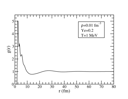
Figure 1: Neutron-neutron correlation function $g(r)$ at a density of $\rho\!=\!0.01$ fm^-3, an electron fraction of $Y_{e}\!=\!0.2$, and a temperature of $T\!=\!1$ MeV. This from a simulation with 40,000 nucleons.

The neutron-neutron correlation function $g(r)$ at a baryon density of $\rho\!=\!0.01$ fm^-3 is shown in Fig. 1. The two-neutron correlation function measures the probability of finding a pair of neutrons separated by a fixed distance $r$. A large broad peak is observed in $g(r)$ in the 2-10 fm region; the lack of neutrons with a relative distance of less than $2$ fm is due to the hard core of the potential. The sharper sub-peaks contained in this structure reflect neutron-neutron correlations (nearest neighbors, next-to-nearest neighbors, and so on) within a single cluster. The Coulomb repulsion among protons prevents the clusters from growing arbitrarily large and keeps them apart. The dip in $g(r)$ at $r\!\simeq\!10$ fm is a result of the Coulomb repulsion between clusters. Finally, the small broad peaks near 25-30, 50, and 75 fm reflect correlations among the different clusters.

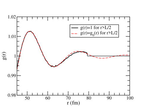
Figure 2: (Color online) The large-$r$ behavior of the two-neutron correlation function displayed in Fig. 1. Note the expanded y-scale. Also shown (red dashed line) is the analytic fit to $g(r)$ according to Eq.(20).

Figure 2 displays an enlargement of the neutron-neutron correlation function for large values of $r$. Finite-size effects lead to an abrupt drop in $g(r)$ at $r\!=\!L/2\!\sim\!80$ fm (not shown). To ensure a reliable estimate of its Fourier transform—and correspondingly of the static structure factor $S(q)$—one must extrapolate $g(r)$ to the region $r\!>\!L/2$. To do so, an analytic function of the following form is fitted to $g(r)$:

$$g_{0}(r)=A_{0}e^{-\alpha_{0}r}\cos(k_{0}r+\delta_{0})+1\;.$$ (20)

The constants $A_{0}$, $\alpha_{0}$, $k_{0}$, and $\delta_{0}$ are obtained from a fit to the large-$r$ behavior of the neutron-neutron correlation function. The result of this fit is indicated by the red dashed line in Fig. 2.

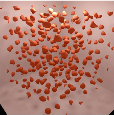
Figure 3: (Color online) The 0.03 fm^-3 proton density isosurface for one configuration of 40,000 nucleons at a density of 0.01 fm^-3. The simulation volume is a cube 159 fm on a side.

Figure 3 shows the 0.03 fm^-3 isosurface of the proton density for one configuration of 40,000 nucleons at a density of $0.01$ fm^-3. All of the protons and most of the neutrons are clustered into nuclei. We discuss the size of these nuclei in Section V. There is also a low density neutron gas between the clusters which is not shown.

The static structure factor $S(q)$ may now be calculated from the Fourier transform of $g(r)$ [see Eq. (17)]. That is,

$$S(q)=1+4\pi\rho_{n}\int_{0}^{\infty}\frac{\sin(qr)}{qr}(g(r)-1)r^{2}dr\;.$$ (21)

In Fig. 4 the static structure factor obtained by using the above extrapolation (i.e., with $g_{0}(r)$ for $r\!\gtrsim\!L/2$) is displayed with the red dashed line. In an earlier publication the static structure factor was calculated directly from the simulation results assuming $g(r)\!=\!1$ for $r\!>\!L/2$ Horowitz et al. (2004). This result is also shown for comparison (black solid line). The improvement in the low-momentum transfer behavior of $S(q)$ is clearly evident. This is important as the value of the static structure factor at zero-momentum transfer $S(q\!=\!0)$ monitors density fluctuations in the system and these may be indicative of a phase transition.

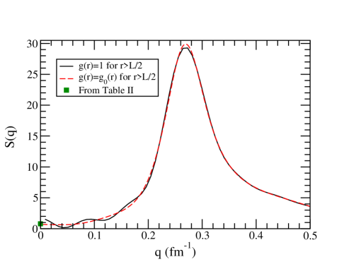
Figure 4: (Color online) Static structure factor $S(q)$ at a density of $\rho\!=\!0.01$ fm^-3, an electron fraction of $Y_{e}\!=\!0.2$, and a temperature of $T\!=\!1$ MeV. The black solid line assumes $g(r)\!=\!1$ for $r\!>\!L/2$ while the red dashed line includes an analytic extrapolation for $g(r)$ for $r\!\gtrsim\!L/2$. The green solid square is the value of $S(0)$ from Eq. (26) and Table 2.

In the limit of zero-momentum transfer the static structure factor $S(q\!=\!0)$ is directly related to the isothermal compressibility. That is Pathria (1996),

$$S(q\!=\!0)=\rho\,k_{\rm B}T\,{\cal K}_{T}=k_{\rm B}T\left(\frac{\partial{P}}{\partial{\rho}}\right)^{-1}_{T}\;,$$ (22)

where the isothermal compressibility is given by

$${\cal K}_{T}^{-1}=-V\left(\frac{\partial{P}}{\partial{V}}\right)_{T}=\rho\left(\frac{\partial{P}}{\partial{\rho}}\right)_{T}\;.$$ (23)

For a classical ideal gas (i.e., $P\!=\!\rho k_{\rm B}T$) the isothermal compressibility reduces to ${\cal K}_{T}^{-1}\!=\!\rho k_{\rm B}T$ and $S(q\!=\!0)\!=\!1$. As expected, in the absence of interactions there are no spatial correlations among the particles. Assuming now that as $q\!\rightarrow\!0$ the fluctuations in the neutron density are proportional to the corresponding fluctuations in the baryon density, one obtains for the static structure factor per neutron

$$S(q\!=\!0)=\frac{N}{A}k_{\rm B}T\left(\frac{\partial{P}}{\partial{\rho}}\right)^{-1}\;.$$ (24)

The derivative of the pressure with respect to the baryon density has not been directly calculated in the simulations. However, the pressure has been computed at various densities and has been tabulated in Table 2. These values can be approximated by a simple fit of the form:

$$P(\rho)=(0.611)\rho+(228.131)\rho^{\alpha+1}\quad(\alpha=1.583)\;,$$ (25)

with the pressure expressed in units of MeV/fm³ and the density in fm^-3. This yields,

$$S(q\!=\!0)\approx\frac{1.358\!\times\!10^{-3}}{\left(1.037\!\times\!10^{-3}+\rho^{\alpha}\right)}\;.$$ (26)

These approximate values for $S(q\!=\!0)$ have been reported in Table 2. For comparison, they have also been added (with a green solid square) to the various figures for which $S(q)$ was directly computed from the Fourier transform of the two-neutron correlation function (see Figs. 4, 8, and 12). Note that there is good agreement between the two approaches.

At low momentum transfers the static structure factor is small because of ion screening. Coulomb correlations—which both hinder the growth of clusters and keep them well separated—screen the weak charge of the clusters thereby reducing $S(q)$. Further, a large peak is seen in $S(q)$ for $q\!\simeq\!0.25$ fm^-1. This corresponds to the coherent scattering from all of the neutrons in a cluster. As we will show in the next section, this peak reproduces coherent neutrino-nucleus elastic scattering at low densities. Finally, the static structure factor decreases for $q\!>\!0.3$ fm^-1. This is due to the form factor of a cluster. As the momentum-transfer increases, the neutrino can no longer scatter coherently form all the neutrons because of the size of the cluster is larger than the neutrino wavelength. All these features will be discussed in greater detail in the next section.

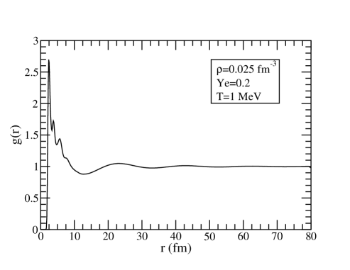
Figure 5: Neutron-neutron correlation function $g(r)$ at a density of $\rho\!=\!0.025$ fm^-3, an electron fraction of $Y_{e}\!=\!0.2$, and a temperature of $T\!=\!1$ MeV. This from a simulation with 100,000 nucleons.

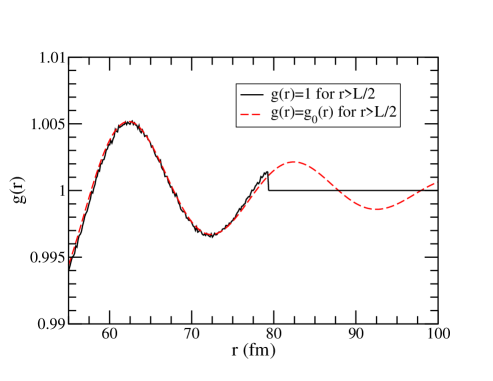
Figure 6: (Color online) The large-$r$ behavior of the two-neutron correlation function displayed in Fig. 5. Also shown (red dashed line) is the analytic fit to $g(r)$.

Next, simulation results are presented at the higher density of $\rho\!=\!0.025$ fm^-3. At this density it becomes much easier to equilibrate the system as protons have shorter distances to move over the Coulomb barriers. In order to minimize finite-size effects more nucleons—a total of $A\!=\!100,000$—are used for these simulations. The two-neutron correlation function is shown in Fig. 5, with its behavior at large distances amplified in Fig. 6. Note that the calculation for $g(r)$, which proceeds by histograming distances between the $N(N\!-\!1)/2$ pairs of neutrons, is now considerably more time consuming. The resulting static structure factor is shown in Fig. 8. The peak in $S(q)$ has now moved to larger $q$ because of the shorter distance between clusters.

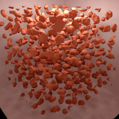
Figure 7: (Color online) The 0.03 fm^-3 proton density isosurface for one configuration of 100,000 nucleons at a density of 0.025 fm^-3. The simulation volume is a cube 159 fm on a side.

Figure 7 shows the 0.03 fm^-3 isosurface of the proton density for one configuration of 100,000 nucleons at a density of $0.025$ fm^-3. All of the protons and most of the neutrons are clustered into nuclei. The size of these nuclei is now larger than at a density of $0.01$ fm^-3 as discussed in Section V. There is also a low density neutron gas between the clusters which is not shown.

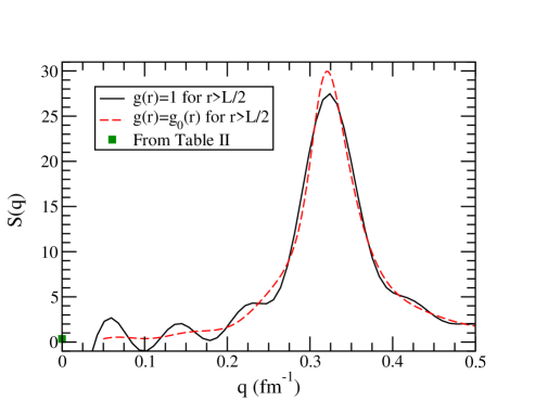
Figure 8: (Color online) Static structure factor $S(q)$ at a density of $\rho\!=\!0.025$ fm^-3, an electron fraction of $Y_{e}\!=\!0.2$, and a temperature of $T\!=\!1$ MeV. The black solid line assumes $g(r)\!=\!1$ for $r\!>\!L/2$ while the red dashed line includes an analytic extrapolation for $g(r)$ for $r\!\gtrsim\!L/2$. The green solid square is the value of $S(0)$ from Eq. (26) and Table 2.

Simulations have also been performed at a density of $\rho\!=\!0.05$ fm^-3 using $A\!=\!100,000$ nucleons. The two-neutron correlation function, together with its amplification at large values of $r$, are shown Figs. 9 and 10, respectively. The corresponding static structure factor is displayed Fig. 12. Note the significant improvement in the behavior of $S(q)$ at low momentum transfers as the sharp cutoff in $g(r)$ is removed in favor of a smooth extrapolation [see Eq. (20)]. As the density increases, and thus the separation between clusters decreases, the peak in $S(q)$ continues to move to higher $q$. However, the peak value of $S(q)$ has now been reduced because of the increase in ion screening with density.

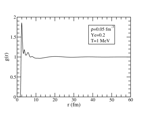
Figure 9: Neutron-neutron correlation function $g(r)$ at a density of $\rho\!=\!0.05$ fm^-3, an electron fraction of $Y_{e}\!=\!0.2$, and a temperature of $T\!=\!1$ MeV. This is from a simulation with 100,000 nucleons.

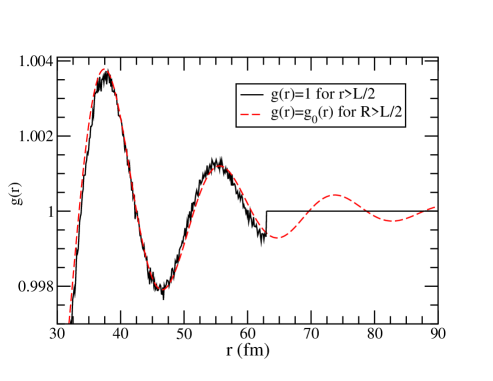
Figure 10: (Color online) The large-$r$ behavior of the two-neutron correlation function displayed in Fig. 9. Also shown (red dashed line) is the analytic fit to $g(r)$.

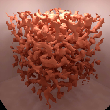
Figure 11: (Color online) The 0.03 fm^-3 proton density isosurface for one configuration of 100,000 nucleons at a density of 0.05 fm^-3. The simulation volume is a cube 126 fm on a side.

Figure 11 shows the 0.03 fm^-3 isosurface of the proton density for one configuration of 100,000 nucleons at a density of $0.05$ fm^-3. The clusters are now seen to have very elongated shapes. The low density neutron gas between these clusters is not shown.

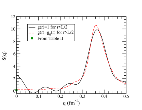
Figure 12: (Color online) Static structure factor $S(q)$ at a density of $\rho\!=\!0.05$ fm^-3, an electron fraction of $Y_{e}\!=\!0.2$, and a temperature of $T\!=\!1$ MeV. The black solid line assumes $g(r)\!=\!1$ for $r\!>\!L/2$ while the red dashed line includes an analytic extrapolation for $g(r)$ for $r\!\gtrsim\!L/2$. The green solid square is the value of $S(0)$ from Eq. (26) and Table 2.

We conclude this section by presenting results for the two-neutron correlation function at a density of $\rho\!=\!0.075$ fm^-3 using a total of $A=40,000$ nucleons in Fig. 13. Note that this is the largest density considered in this work. At this density the clusters have been “melted” and the system has evolved into a uniform phase. In Fig. 14 results for the static structure factor at this density are compared with the corresponding results at the lower densities. There is no longer evidence for a large peak in $S(q)$ in the uniform system as a consequence of the complete loss in coherence. Finally, Fig. 15 shows $S(q)$ at large momentum transfers. One observes that the static structure factor decreases with increasing density in the intermediate $q$-region before approaching the value of one (as it must) at high $q$.

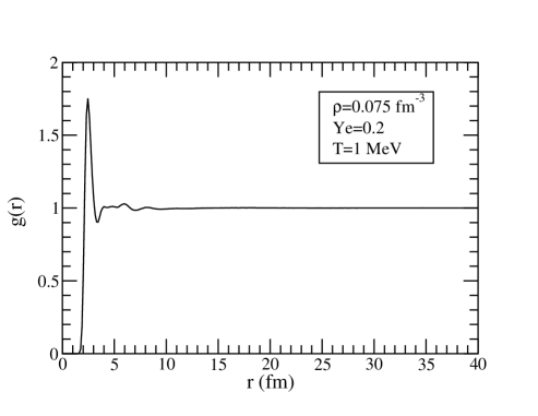
Figure 13: Neutron-neutron correlation function $g(r)$ at a density of $\rho\!=\!0.075$ fm^-3, an electron fraction of $Y_{e}\!=\!0.2$, and a temperature of $T\!=\!1$ MeV. This from a simulation with 40,000 nucleons.

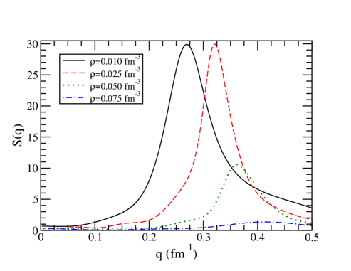
Figure 14: (Color online) Static structure factor $S(q)$ for a variety of densities at an electron fraction of $Y_{e}\!=\!0.2$ and a temperature of $T\!=\!1$ MeV. The black solid line is for a density of $\rho\!=\!0.01$ fm^-3, while the red dashed line is for $\rho\!=\!0.025$ fm^-3, the green dotted line for $\rho\!=\!0.05$ fm^-3, and the blue dot-dashed line for $\rho\!=\!0.075$ fm^-3.

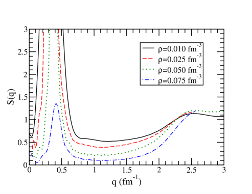
Figure 15: (Color online) The large-$q$ behavior of the static structure function displayed in Fig. 14.

In the next section we will compare these “complete” results with conventional approaches that model the system as a collection of strongly-correlated, neutron-rich nuclei plus a neutron gas. In this approach the peak observed in the static structure factor is attributed to neutrino-nucleus elastic scattering. Note, however, that the complete simulation results obtained in this section should remain valid even when these nuclear models break down.

V Cluster Model

In this section a cluster model is developed with the goal of comparing our simulation results from the previous section with commonly used approaches. In the complete model employed earlier, trajectories for all the nucleons were calculated from molecular dynamics simulations and these were used to compute directly the two-neutron correlation function and its corresponding static structure factor. One of the main virtues of such an approach is that there is no need to decide if a given nucleon is part of a cluster or part of the background vapor. Nevertheless, in this section a clustering algorithm is constructed with the aim of assigning nucleons to clusters. In this way one can compare the inferred composition extracted from our simulations with many nuclear statistical equilibrium (NSE) models that describe the system as a collection of nuclei and free nucleons. In this way one can then compare the static structure factor extracted from the complete simulations with that calculated in these NSE models.

V.1 Clustering Algorithm

The clustering algorithm implemented in this section assigns a nucleon to a cluster if it is within a distance $R_{C}$ of at least one other nucleon in the cluster. In practice, one stars with a given nucleon and searches for all of its “neighbors”, namely, all other nucleons contained within a sphere of radius $R_{C}$. Next, one repeats the same procedure for all of its neighbors until no new neighbors are found. This procedure divides a fixed configuration of nucleons into a collection of various mass clusters (ı.e., “nuclei”).

To illustrate this procedure the final nucleon configuration of the complete simulation of the previous section at a density of $\rho=0.01$ fm^-3 is selected after the system has evolved for a total time of $t_{\rm f}\!=\!1,287,000$ fm/c. Having selected a cutoff radius of $R_{C}\!=\!3$ fm, one finds that the 40,000 nucleons in the system are divided in the following way: a) 11,062 free neutrons, b) no free protons, c) a few light nuclei with $A\!<\!8$, and d) a collections of heavy nuclei with a mass distribution of $50\!\lesssim\!A\!\lesssim\!160$. The mass-weighted average of all clusters with $A\!>\!2$ is equal to $\langle A\rangle\!=\!99$. This distribution of clusters is displayed in Fig. 16 and listed in Table 3.

Table 3: Distribution of cluster as a function of the cutoff radius $R_{C}$ at a density $\rho\!=\!0.01$ fm^-3 for a system of 40,000 nucleons. The number of free neutrons is denoted by $N(A\!=\!1)$, the average mass of all $A\!>\!2$ clusters by $\langle A\rangle$, and the size of the largest cluster by $A_{\rm max}$.

$R_{C}$ (fm)	$N(A\!=\!1)$	$\langle A\rangle$	$A_{\rm max}$
2.0	20,585	46.20	118
2.5	14,233	102.29	155
3.0	11,062	98.75	160
3.5	7,856	96.17	254
4.0	5,131	100.97	261
4.5	2,888	149.84	513
5.0	1,427	14,069	23,189

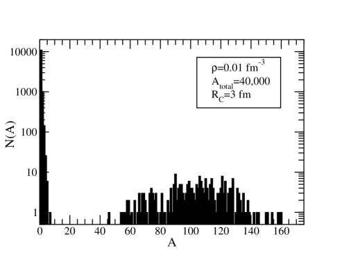
Figure 16: Number of clusters of atomic mass $A$ for one configuration of 40,000 nucleons at a density of $\rho\!=\!0.01$ fm^-3. Note that this is a linear-log plot.

In Table 3 results are also displayed for values of the cutoff radius in the 2-5 fm range. Note that the average cluster mass $\langle A\rangle$ appears remarkably constant for $2.5\!\leq\!R_{C}\!\leq\!4$ fm. This suggest that any value of $R_{C}$ within this range should give similar results. However, if $R_{C}$ is chosen too large, for example $R_{C}\!=\!5$ fm, then most of the nucleons become part of one single giant cluster.

Similar results for a density of $\rho\!=\!0.025$ fm^-3 are presented in Table 4. This distribution is extracted from the final configuration of 100,000 nucleons obtained after a total evolution time of $t_{\rm f}\!=\!52,000$ fm/c. Using a cutoff radius of $R_{C}=3$ fm, the 100,000 nucleons in the system are now divided into 14,549 free neutrons, no free protons, a few light nuclei, and a broad collection of heavy nuclei with $A$ from about 80 to 614 nucleons. Such a distribution is shown in Fig. 17. The average mass has now grown to $\langle A\rangle\!=\!199$. The mass of the heavy nuclei is seen to increase with density as shown in Fig. 17. Finally, results at $\rho\!=\!0.05$ fm^-3 are presented in Table 5. Now the density is so high that it is difficult to design a sensibly scheme to divide the system into clusters, see Fig. 11. For example, even with a cutoff radius as small as $R_{C}\!=\!2.5$ fm, already 78,178 of the 100,000 nucleons become part of a single giant cluster.

Table 4: Distribution of cluster as a function of the cutoff radius $R_{C}$ at a density $\rho\!=\!0.025$ fm^-3 for a system of 100,000 nucleons. The number of free neutrons is denoted by $N(A\!=\!1)$, the average mass of all $A\!>\!2$ clusters by $\langle A\rangle$, and the size of the largest cluster by $A_{\rm max}$.

$R_{C}$ (fm)	$N(A\!=\!1)$	$\langle A\rangle$	$A_{\rm max}$
2.0	49,761	58.95	162
2.5	28,234	167.40	423
3.0	14,549	198.91	614
3.5	5,187	59,411	75,003

Table 5: Distribution of cluster as a function of the cutoff radius $R_{C}$ at a density $\rho\!=\!0.05$ fm^-3 for a system of 100,000 nucleons. The number of free neutrons is denoted by $N(A\!=\!1)$, the average mass of all $A\!>\!2$ clusters by $\langle A\rangle$, and the size of the largest cluster by $A_{\rm max}$.

$R_{C}$ (fm)	$N(A\!=\!1)$	$\langle A\rangle$	$A_{\rm max}$
2.0	47,239	56.86	308
2.5	16,219	72,952	78,178

Figure 17: (Color online) Number of clusters of atomic mass $A$ for one configuration of 100,000 nucleons at a density of $\rho\!=\!0.025$ fm^-3 (black hatched line). Also shown for comparison is the number of clusters (from Fig. 16) at $\rho\!=\!0.01$ fm^-3 (red solid line). Note that both scales are now linear.

V.2 Cluster Form Factors

To describe coherent neutrino scattering from a single cluster, that is, neutrino-nucleus elastic scattering, one must calculate the elastic form factor for the cluster. This is given by

$$F(q)=\frac{1}{N}\sum_{n=1}^{N}\frac{\sin(qr_{n})}{qr_{n}}\;.$$ (27)

Here the sum runs over the $N$ neutrons in the cluster and $r_{n}$ is distance from the n_th neutron to the center of mass of the $N$-neutron system. The form factor represents the Fourier transform of the point neutron density and here, for simplicity, has been averaged over the direction of the momentum transfer. Note that the elastic form factor is normalized so that $F(q\!=\!0)\!=\!1$. In Fig. 18 the elastic form factors of all clusters with $A\!>\!10$ are displayed at a density of $\rho\!=\!0.01$ fm^-3 (a cutoff radius of $R_{C}\!=\!3$ fm was selected). The large spread in the form factors reflects the many different sizes of the individual clusters (see Fig. 16). Indeed, the root-mean-square (RMS) radius of a cluster appears to scale approximately as $A^{1/3}$. Therefore, in Fig. 19 all of these form factors are plotted but against a scaled momentum transfer $qA^{1/3}$. Now all the (scaled) form factors fall in a fairly narrow band suggesting that, while these neutron-rich clusters have different radii, they all share a similar shape.

In Fig. 20 we display the form factor for a single neutron-rich cluster with $A=100$ and $Z=28$ (“¹⁰⁰Ni”) extracted from the simulation with a density of $\rho\!=\!0.01$ fm^-3. Also shown in the figure (with a green dotted line) is the form factor $F_{0}(q)$ of a uniform neutron distribution with a sharp surface radius $R_{n}$ chosen to reproduce the RMS radius of the neutron-rich cluster $<r_{n}^{2}>^{1/2}$. It is given by

$$F_{0}(q)=3\frac{\sin(x)-x\cos(x)}{x^{3}}\quad(x\equiv qR_{n})\;,$$ (28)

with $R_{n}$ given by

$$R_{n}=\sqrt{\frac{5}{3}}\langle r_{n}^{2}\rangle^{1/2}\;.$$ (29)

Finally, Fig. 20 also shows the neutron form factor of the exotic, neutron-rich nucleus ⁹⁸Ni calculated in a relativistic mean-field approximation using the very successful NL3 interaction Lalazissis et al. (1997). While the NL3 form factor has a slightly smaller RMS radius, the overall agreement between all three models is fairly good. Note that ⁹⁸Ni (rather than ¹⁰⁰Ni) was used in this calculation as it contains closed protons and neutrons subshells. For this exotic nucleus the $1h^{11/2}$ neutron orbit—responsible for magic number 82—is not even bound.

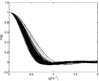
Figure 18: Cluster form factor $F(q)$ as a function of the momentum transfer $q$ for all clusters with $A\!>\!10$ using a single configuration of 40,000 nucleons at a density of $\rho\!=\!0.01$ fm^-3.

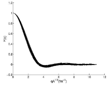
Figure 19: Cluster form factor $F(q)$ as a function of the scaled momentum transfer $qA^{1/3}$ for all clusters with $A\!>\!10$ using a single configuration of 40,000 nucleons at a density of $\rho\!=\!0.01$ fm^-3.

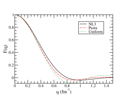
Figure 20: (Color online) Cluster form factor $F(q)$ as a function of the momentum transfer $q$. The red dashed line represents the angle-averaged form factor for one cluster with $A\!=\!100$ and $Z\!=\!28$ from a simulation at a density of $\rho\!=\!0.01$ fm^-3. The dotted (green) line is the form factor of a uniform density sphere with the same root-mean-square radius [see Eqs. (28) and (29)]. Finally, the solid line is the form factor of the very neutron-rich nucleus ⁹⁸Ni calculated in a relativistic mean-field approximation with the NL3 interaction Lalazissis et al. (1997).

The clusters generated in the simulations are neutron-rich nuclei with well developed neutron skins. Nuclei with neutron skins are characterized by neutron radii that are larger than those for the protons. Using the distribution of nuclei obtained with a density of $\rho\!=\!0.01$ fm^-3, the following values are obtained for average matter, proton, and neutron RMS radii respectively:

$$\langle r^{2}\rangle^{1/2}=1.06\,A^{1/3}\,{\rm fm}\;,$$ (30a)

$$\langle r_{p}^{2}\rangle^{1/2}=0.91\,A^{1/3}\,{\rm fm}\;,$$ (30b)

$$\langle r_{n}^{2}\rangle^{1/2}=1.11\,A^{1/3}\,{\rm fm}\;.$$ (30c)

Note that the sharp-surface radius of a uniform distribution with the same RMS radius is simply given by $(5/3)^{1/2}$ times these values [see Eq. (29)].

V.3 Single Heavy Nucleus Approximation

A number of approaches to dense matter, such as those using the equation of state by Lattimer and Swesty Lattimer and Swesty (1992), model the system as a collection of free neutrons plus a single representative heavy nucleus. Occasionally, free protons and alpha particles are also added to the system. To mimic this approach, a model is constructed based on our earlier cluster results reported in Tables 3 and 4 for a cutoff radius of $R_{C}\!=\!3$ fm. For example, at a density of $\rho\!=\!0.01$ fm^-3 the system contains a mass fraction $X_{n}\!=\!0.28$ of free neutrons and a mass fraction of $X_{h}\!=\!1-X_{n}\!=\!0.72$ for the single representative heavy nucleus. According to the average mass reported in Table 3, a mass of $A\!=\!100$ is assigned to this representative heavy nucleus. Conservation of charge constrains this nucleus to have $Z\!\approx\!28$. Note that due to the presence of free neutrons (but not free protons) the charge-to-mass ratio of the heavy nucleus $Z/A\!=\!0.28$ slightly exceeds the electron fraction $Y_{e}\!=\!0.2$ of the whole system. The assumed composition of the system at densities of $\rho\!=\!0.01$ fm^-3 and $\rho\!=\!0.025$ fm^-3 is given in Table 6.

Table 6: Composition of the system in the single-heavy-nucleus approximation. The mass fraction of free neutrons is denoted by is $X_{n}$ and that of heavy nuclei by $X_{h}$. The mass and charge of the nuclei are given by $A$ and $Z$, respectively. Finally, the radii of the equivalent uniform proton and neutron distributions are denoted by $R_{p}$ and $R_{n}$, respectively.

$\rho$ (fm-3)	$X_{n}$	$X_{h}$	A	Z	$R_{p}$ (fm)	$R_{n}$ (fm)
0.010	0.28	0.72	100	28	5.45	6.68
0.025	0.14	0.86	199	47	6.84	8.40

The heavy nuclei are assumed to interact exclusively via a screened Coulomb interaction. Each nucleus is assumed to have a uniform charge distribution $\rho_{\rm ch}$ that extends out to a radius $R_{p}$ chosen to reproduce the proton RMS radius $\langle r_{p}^{2}\rangle^{1/2}$ given in Eq. (30). The Coulomb interaction between two such nuclei whose centers are separated by a distance $R$ is given by

$$V_{C}(R)=e^{2}\int d^{3}r\,\rho_{\rm ch}(r)\int d^{3}r^{\prime}\,\rho_{ch}(r^{\prime})\frac{e^{-R_{\rm tot}/\lambda}}{R_{\rm tot}},$$ (31)

where $R_{\rm tot}\equiv|{\bf R}+{\bf r}-{\bf r}^{\prime}|$ and $\lambda$ is the screening length fixed (as in Sec. II) at a constant value of $\lambda\!=\!10$ fm. In the limit that the distance between nuclei is much larger than the nuclear RMS radius (i.e., $R_{p}\!\ll\!R$) the above integral reduces to

$$V_{C}(R)\simeq e^{2}\rho_{\rm ch}^{2}\frac{e^{-R/\lambda}}{R}\Big{(}\int d^{3}r\,e^{-r\cos\theta/\lambda}\Big{)}^{2}$$

$$\phantom{V_{C}(R)}=\frac{Z^{2}e^{2}}{R}e^{-R/\lambda}f(R_{p}/\lambda)\;,$$ (32)

where the dimensionless function $f(x)$ has been defined as follows:

$$f(x)=\left[3\frac{x\cosh(x)-\sinh(x)}{x^{3}}\right]^{2}\quad(x\equiv R_{p}/\lambda)\;.$$ (33)

Note that the function $f$ is independent of $R$. Indeed, it only depends on the dimensionless ratio $R_{p}/\lambda$, namely, on the interplay between the nuclear size and the screening length. In the absence of screening, $f\!\equiv\!1$ (independent of nuclear size) in accordance with Gauss’ law. However, with screening $f$ becomes greater than one. The finite nuclear size places some of the charges closer together than $R$; this increases the repulsion. Of course, the finite size also places some of the charges farther apart, thereby decreasing the repulsion. When these two effects are weighted by the screening factor $e^{-r/\lambda}$, the repulsion more than compensates for the “attraction” leading ultimately to $f\!\geq\!1$. In the particular case of $R_{p}\!=\!5.45$ fm and $\lambda\!=\!10$ fm, one obtains $f(0.545)\!=\!1.061$ (about a 6% increase).

The single-heavy-nucleus models consists of a gas of noninteracting neutrons plus ions interacting via the screened Coulomb interaction given in Eqs. (32). Molecular dynamics simulations in the ion coordinates are performed to compute its static structure factor $S_{\rm ion}(q)$. The simulations used 5,000 to 10,000 ions and a time step of 25 to 75 fm/c. The ion simulation can afford a larger time step than the corresponding nucleon simulation because the heavier ions move slower. Further, the ion simulations require fewer particles to simulate the same physical volume because each ion “contains” several nucleons. The static structure factor for the ions computed in this way (for densities of $\rho\!=\!0.01$ fm^-3 and $\rho\!=\!0.025$ fm^-3) is shown in Fig. 21.

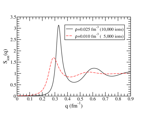
Figure 21: (Color online) Ion static structure factor $S_{\rm ion}(q)$ as a function of the momentum transfer $q$. The black solid line is from of a simulation with 10,000 ions corresponding to a density of $\rho\!=\!0.025$ fm^-3. The red dashed line is from a simulation with 5,000 ions corresponding to a density of $\rho\!=\!0.01$. See text for details.

Neutrino scattering from this system is described, in this single-heavy-nucleus model, by neutrino-nucleus elastic scattering within a framework that incorporates effects from both, the nuclear form factor and ion screening from the correlated nuclei. The cross section for elastic neutrino scattering from a single nucleus is proportional to the square of the weak charge of the nucleus times a suitable form factor to account for it finite size. For the weak charge of the nucleus we simply use its neutron number $N$ as we continue to ignore the small weak charge of the proton, i.e., ${\cal Q}_{\rm weak}\!=\!-N\!+\!Z(1\!-\!4\sin^{2}\theta_{\rm W})\rightarrow-N$. Thus, the weak nuclear form factor reduces to that of the neutron distribution. Further, to incorporate effects that result from correlations among the ions, such as ion screening, the cross section is multiplied by the ion static structure factor $S_{\rm ion}(q)$. Finally, one multiplies these terms by the fraction $X_{h}$ of heavy nuclei and divides by $N$ to obtain a static structure factor per neutron $S_{\rm model}(q)$ consistent with the normalization of the earlier sections. That is,

$$S_{\rm model}(q)=X_{h}NF(q)^{2}S_{\rm ion}(q)\;.$$ (34)

Note that in addition to the coherent nuclear contribution there is a small incoherent contribution from the neutron gas that has been neglected. As defined above, this static structure factor can now be directly compared to the one obtained in the full nucleon simulations. This prescription for $S_{\rm model}(q)$ corresponds to what is presently used in most supernova simulations. These simulations often take $X_{h}$ and $N$ from the Lattimer-Swesty equation of state Lattimer and Swesty (1992) and $S_{\rm ion}(q)$ as computed in Ref. Horowitz (1997).

In Fig. 22 the model static structure factor $S_{\rm model}(q)$ is compared to the one from the full nucleon calculation (see Sec. IV) at a density of $\rho\!=\!0.01$ fm^-3. The uniform form factor of Eq. (28) is used with the sharp surface radius $R_{n}$ listed in Table 6. For low to moderate momentum transfers the agreement between the two approaches is excellent. This indicates that—at this density and (low) momentum transfers—the system is well described by a collection of nuclei of a single average mass. We expect that this good agreement will also hold at lower densities. However, there is a modest disagreement between $S_{\rm model}(q)$ and the complete $S(q)$ for $q\!>\!0.25$ fm^-1. This provides the first indication of limitations within the single heavy nucleus approximation. The discrepancy could arise because the broad distribution of cluster sizes displayed in Fig. 16 is approximated by a single average cluster with a mass of $A=100$. Or it could be due to a breakdown in the factorization scheme. That is, the cross section may no longer factor into a product of a correlation function between ions ($S_{\rm ion}$) times the weak response of a single ion ($N^{2}F(q)^{2}$).

A similar comparison is done in Fig. 23 but now at the higher density of $\rho\!=\!0.025$ fm^-3. Now the disagreement between $S_{\rm model}(q)$ and $S(q)$ is more severe. This indicates that errors in the single nucleus approximation will grow rapidly with density. Moreover, the single nucleus approximation overpredicts the neutrino opacity relative to the complete calculations.

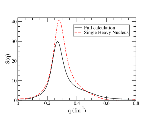
Figure 22: (Color online) Neutron static structure factor $S(q)$ as a function of the momentum transfer $q$ at a density of $\rho\!=\!0.01$ fm^-3 for the full calculation (black solid line). Also shown (red dashed line) is the prediction from the ion static structure factor in Fig. 21 including the square of the cluster form factor, as explained in the text.

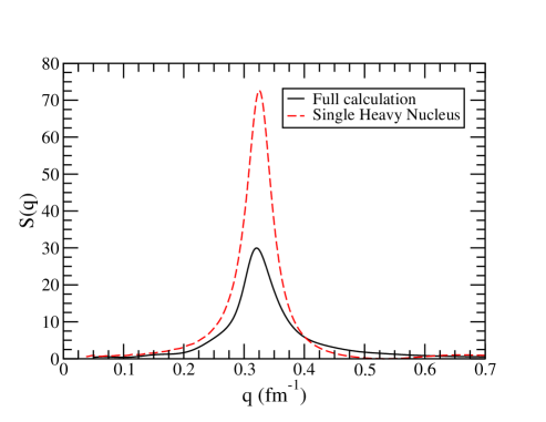
Figure 23: (Color online) Neutron static structure factor $S(q)$ as a function of the momentum transfer $q$ at a density of $\rho\!=\!0.025$ fm^-3 (black solid line). Also shown (red dashed line) is the prediction from the ion static structure factor in Fig. 21 including the square of the cluster form factor, as explained in the text.

VI Conclusions

Nonuniform neutron-rich matter was studied via semiclassical simulations with an interaction that reproduces the saturation density and binding energy of nuclear matter and incorporates the long-range Coulomb repulsion between protons. Simulations with a large number of nucleons (40,000 to 100,000) enable the reliable determination of the two-neutron correlation function and its Fourier transform—the static structure factor—even for low momentum transfers. The static structure factor $S(q)$ describes coherent neutrino scattering that is expected to dominate the neutrino opacity. At low momentum transfer $q$ the static structure factor is small because of ion screening; correlations between different clusters screen the weak charge. At intermediate momentum transfers a large peak is developed in $S(q)$ corresponding to coherent scattering from all of the neutrons in a cluster. This peak moves to higher $q$ and decreases in amplitude as the density of the system increases.

In principle the neutrino opacity could be greatly increased by large density fluctuations. A simple first-order phase transition has a two-phase coexistence region where the pressure is independent of density. Large density fluctuations in this region imply a very large value of the static structure factor at very small momentum transfers. Indeed, $S(q\!=\!0)$ is directly proportional to the density fluctuations in the system. Moreover, density fluctuations are also proportional to the isothermal compressibility. For consistency, the static structure factor $S(q\!=\!0)$ was computed in these two equivalent yet independent ways, namely, as the Fourier transform of the two-neutron correlation function and as the derivative of the pressure with respect to the baryon density. While we find good agreement between these two schemes, no evidence is found in favor of a large enhancement in $S(q\!=\!0)$. We conclude that the system does not undergo a simple, single component first-order phase transition, so no large increase in the neutrino opacity was found.

To compare our simulation results to more conventional approaches of wide use in supernova calculations a cluster model was introduced. A minimal spanning tree clustering algorithm was used to determine the composition of the various clusters (“nuclei”) in the simulations (see for example Ref. Papadimitriou and Kenneth Steiglitz (1998)). To make contact with some of these conventional approaches, such as the single heavy nucleus approximation, the neutrino opacity was computed in a system modeled as a gas of free neutrons and a representative (i.e., average) single-species heavy nucleus. The neutrino opacity for such a system is dominated by elastic scattering from the heavy nucleus. The contribution from the single nucleus to the neutrino response is proportional to the square of its weak charge (assumed to be carried exclusively by the neutrons) and its elastic neutron form-factor, that accounts for its finite size. Further, Coulomb correlations among the different nuclei was incorporated through an ion static structure factor to account for ion screening. Fairly good agreement is found between the single heavy nucleus approximation and our complete simulations at low density and especially at small momentum transfers. However, starting at a density of approximately $10^{13}$ g/cm³, we find a large disagreement between the two approaches that grows rapidly with increasing density. In particular, our complete simulations yield neutrino opacities that are smaller than those in the single heavy nucleus approximation. Note that our full simulations yield accurate results even at the (high) densities where the single heavy nucleus approximation becomes invalid. We reiterate that the single heavy nucleus approximation is what is presently employed in most supernova simulations.

Future work could include calculating the dynamical response of the system to study the transfer of energy between neutrinos and matter. Note that a great virtue of molecular dynamics approaches combined with special purpose computers (such as what has been done here) is that dynamical information for systems with large number of particles may be readily obtained from time-dependent correlations. Particularly interesting is the low-energy part of the response which should be dominated by the so-called Pygmy resonances. These oscillations of the neutron skin of neutron-rich nuclei against the symmetric core should be efficiently excited by low-energy neutrinos. Another promising area for future research is the spin response of the system. A first step could involve including spin dependent forces in our model. The spin response is interesting because nucleons have large spin dependent couplings to neutrinos.

*

Appendix A MDGRAPE

To do the simulations we used a special purpose computer called the MDGRAPE-2. The MDGRAPE-2 is a single board which plugs into the PCI bus of a general purpose computer, and is designed for extremely fast calculation of forces and potentials in molecular dynamics simulations Narumi et al. (1999). It is the third generation of such hardware, which evolved from the work of J. Makino et al at the University of Tokyo on similar hardware called the GRAPE (for GRAvity PipE), for doing gravitational N-body problems Makino et al. (2000). In our case, we have two boards plugged into the PCI bus of one of the Power3+ nodes of Indiana University’s IBM SP supercomputer. Each board is rated at a peak speed of 64 GigaFLOPS (floating point operations per second). The MDGRAPE-2 can compute any central potential of the form

$$V(i,j)=b_{ij}f(a_{ij}(r_{ij}^{2}+\epsilon_{ij}^{2}))$$ (35)

or the corresponding central force, which is of the same form, except multiplied by $\mathbf{r}$. All three terms in (2) are of this form. In our case $\epsilon_{ij}=0$, and $b_{ij}$ and $a_{ij}$ are either scalars, or $2\times 2$ matrices, corresponding to the two particle types proton and neutron. The boards are accessed via the M2 library, which the user links into his code. The library is very easy to use, and handles distribution of work between the two MDGRAPE-2 boards without user intervention. The user defines $f(x)$ by a function table of 1024 points, which the MDGRAPE-2 interpolates via fourth degree polynomial interpolation. One can thus reproduce most physically realistic functions very accurately. Software is provided for constructing function tables, which are stored in files and loaded in during runtime.

At each MD time step, one calls M2 subroutines to load in the function table and the scale factors or matrices $a_{ij}$ and $b_{ij}$. One then calls a subroutine to load in the source particle coordinates, and subroutines to load integer arrays of particle types (0 for neutron, 1 for proton) for both source and target particles. Then one calls a force calculation routine, passing it the array of target particle coordinates. In our case the source and target particles are the same, but they do not have to be. One input parameter to the force calculation specifies that periodic boundary conditions should be used. The MDGRAPE-2 has built in hardware for taking periodic b.c. into account. The output is an array containing the total force on each target particle. A similar call can be made to compute the total potential energy of each particle.

We must go through these steps three times, once for each term in (2). Still, the MDGRAPE-2 is much faster than serial Fortran code. In ordinary Fortran, this whole calculation would be done in a pair of nested DO loops, and thus would take of order $O(A^{2})$ time. For our simulations with $A=40,000$ this would be prohibitive even for today’s fast CPUs. But the two MDGRAPE-2 boards together can do the force calculation about 90 times faster than a single Power3+ processor, so that a simulation of 100,000 MD time steps that would take over two years using a serial program can be done in less than nine days. Benchmark tests show this speedup holds out to at least $A=160,000$. Each MDGRAPE-2 board has enough memory to hold a half million particles, so we have not yet reached our maximum capability.

We calculated the neutron-neutron correlation function $g(r)$ (see below) using ordinary Fortran code, as it was not clear how to perform this calculation with the MDGRAPE-2. Although $g(r)$ is also an $O(A^{2})$ calculation, it is done infrequently, and does not severely impact performance.