CMB Quadrupole induced polarisation from clusters and filaments

We present the estimates of the Cosmic Microwave Background (CMB) polarisation power spectrum from galaxy clusters and filaments using hydrodynamical simulations of large scale structure formation. We focus in the present study on the CMB Quadrupole induced polarisation, which is the dominate secondary polarisation effect, and give the E and B mode power spectra between $l\sim 560$ to $20000$.

1 Introduction

After recombination, the CMB photons scatter off free electrons in ionised matter, such as the hot gas trapped in the potential wells of galaxy clusters. The presence of the CMB temperature quadrupole induces a linear polarisation in the scattered radiation.

Sunyaev and Zel’dovich $\!{}^{{\bf?}}$ were the first to estimate the level of polarisation in galaxy clusters. These authors pointed out that in addition to the primary CMB quadrupole there are two other sources of temperature quadrupole seen by a cluster: a quadrupole due to the transverse peculiar velocity of the cluster and double scattering. Studying the induced CMB polarisation due to clusters can open a whole new window for cosmology. Sunyaev and Zel’dovich proposed to use the polarisation to estimate cluster’s transverse velocity. Measuring the polarisation towards distant clusters should provide us with an opportunity to observe the evolution of the CMB quadrupole $\!{}^{{\bf?}}$. Moreover, CMB quadrupole seen by the clusters contains statistical information on the last scattering surface of at the cluster position. Therefore, measuring the cluster polarisation should help us to beat the cosmic variance $\!{}^{{\bf?},{\bf?}}$.

In this work, we study the polarisation induced by galaxy clusters. We focus in the statistical properties of such a polarised signal by computing its angular power spectrum at small angular scales. We explore the signal associated with the primary CMB temperature quadrupole since it dominates at the scales we are interested in $\!{}^{{\bf?}}$. To do so, we follow the method of Liu et al. $\!{}^{{\bf?}}$, in which the authors computed the polarised signal at reionisation using N-body simulations in combination with an analytical description to model the gas distribution. Based on the same formulae and similar approach, we estimate the polarisation from the hot gas in galaxy clusters and the warm gas in filaments using hydrodynamical simulations of large scale structure (LSS), which directly account for the gas dynamics.

In Section 2 we describe the method of this work. We briefly review the formulae of the polarisation power spectra and the hydrodynamical simulations used in this paper. In Section 3, we present the results of our work and give a discussion and conclusion in Section 4.

2 Background

The polarisation signal is usually described by the Stokes parameters which can be combined to obtain a divergence free component, the so-called $E$ mode, and a curl component, the so-called $B$ mode.

The power spectra of polarisation of E and B modes are obtained by integrating the product of the visibility function $g$ and the polarisation source. In the case of primary polarisation, the source is the quadrupole of the primary CMB temperature anisotropies. This is a first order signal. When dealing with second order effects, one has to take into account possible modulations of the visibility function by the electron density perturbations. This was done in Liu et al. $\!{}^{{\bf?}}$. More specifically, the power spectra were found to be:

$$C_{(E,B)l}=(4\pi)^{2}\frac{9}{16}\frac{(l+2)!}{(l-2)!}\sum_{m}\int k^{2}{\rm d}k\left\langle\left|\int{\rm d}\tau g(\tau)\delta_{e}({\bf k},\tau)Q^{(m)}({\bf k},\tau)T_{(E,B)l}^{(m)}(kr)\right|^{2}\right\rangle,$$ (1)

where $\delta_{e}({\bf k},\tau)$ is the electron density perturbation as a function of scale $\bf k$ and conformal time $\tau$, and $Q^{(m)}=\sqrt{\frac{4\pi}{5}}\int{\rm d}^{3}{\bf k}\Delta^{(m=0)}_{T2}({\bf k})Y_{2}^{m*}(\hat{\bf k})$ is the projected scalar mode of primary CMB quadrupole ($\Delta^{(m=0)}_{T2}$) in the frame of $\delta_{e}$. The visibility function $g(\tau)$ has a simple physical meaning, being the probability that a photon had its last scattering at epoch $\tau$ and reaches the observer at the present time, $\tau_{0}$. It is defined as $g(\tau)\equiv-\frac{{\rm d}\kappa}{{\rm d}\tau}{\rm e}^{\kappa(\tau_{0})-\kappa(\tau)}$, where $\kappa({\tau})$ is the electron-scattering optical depth at time $\tau$. The term $T_{(E,B)l}^{(m)}(kr)$ is given by the combination of the spherical Bessel functions (for details see Table 1 in Liu et al. $\!{}^{{\bf?}}$).

In order to calculate the polarisation anisotropy spectra using the formulae mentioned above, we compute the visibility function and the electron density distribution from clusters and filaments using non-radiative hydrodynamical simulations of a $\Lambda$CDM cosmology, with matter density parameter, $\Omega_{{\rm m}}=0.3$, cosmological constant density, $\Omega_{\Lambda}=0.7$, hubble parameter, $h=0.71$, and baryon density, $\Omega_{b}=0.044$. The initial density field was constructed using $160^{3}$ particles of both baryonic and dark matter, perturbed from a regular grid of fixed comoving size $L=100h^{-1}{\rm Mpc}$. The CDM matter power spectrum used in the simulation had a shape parameter, $\Gamma=0.21$, and normalization $\sigma_{8}=0.9$. The run was started at redshift $z=50$ and evolved to $z=0$ using the publicly available Hydra (AP³M/SPH) code $\!{}^{{\bf?},{\bf?}}$. The gravitational softening was fixed at $25\,h^{-1}{\rm kpc}$ in physical units below $z=1$, and above this redshift held constant to $50\,h^{-1}{\rm kpc}$ in comoving co-ordinates.

In the simulation, the gas is assumed ionised if the temperature is higher than $10^{5}$ K. We further define two gas phases based on the baryon collapsed density: when the gas overdensity, $\delta$, is greater than the density contrast at collapse, $\Delta_{c}=178\Omega_{m}(z)^{-0.55}$, the gas is in clusters; the low density phase defined by $5<\delta<\Delta_{c}$ encompasses a warm gas which we call filaments. The visibility function is obtained from the time evolution of the ionisation fraction in our run for $T>10^{5}$ K. For the computation of $C_{(E,B)l}$, we evaluate the electron density fluctuations on a regular grid with $600^{3}$ cells inside the comoving box, which corresponds to a fixed cell separation of $0.17\,h^{-1}{\rm Mpc}$ in comoving coordinates.

Finally, the only remained unknown term is the quadrupole of the temperature anisotropies. Given the cosmological parameters and the ionisation fraction from our simulation, the publicly available code CMBFast $\!{}^{{\bf?}}$ can output the time evolution of the temperature quadrupole component with different ${\bf k}$-basis. Note that the perturbations of tensor mode are such that the normalizations to COBE and to $\sigma_{8}=0.9$, used in our simulation, are consistent. We assume that the tensor spectral index satisfies the single field inflationary consistency condition $n_{t}=-r/8$ with $r$ being the ratio of tensor to scalar quadrupole $r=C^{T}_{l}/C^{S}_{l}$. Here $r=0.05$ and $n_{t}=-0.00625$ are applied when running CMBFast.

3 Power spectra of polarisation of clusters and filaments

We now investigate the contribution to the polarisation power spectra from the two different gas phases defined previously. We show the results in Fig(1). Note that the range of multipoles $l$ is limited by the resolution (for high $l$s) and box size (for low $l$s) of the simulation. The highest multipole $l$ is set by the corresponding angular size of $0.17\,h^{-1}{\rm Mpc}$ at $z=0.72$ in our simulation.

We get the same power for the secondary E and B mode polarisation with a maximum difference is less than $10^{-6}$. The reason for the equality of the total E- and B-mode power spectra is essentially that the first-order quadrupole whose scattering produces the polarisation is dominated by large scales, and so has a random orientation relative to the small-scale fluctuations in the electron density. Scattering of the quadrupole by the small-scale fluctuations therefore on average excites E- and B- modes equally $\!{}^{{\bf?}}$ $\!{}^{{\bf?}}$.

We now compare the polarisation signal from two phases: the cluster and so-called filaments. The power spectrum from all the ionized particles (with $T>10^{5}$ K) is also shown in the figure (1). The two curves for all ionized particles and filaments have similar shapes peaking at $l\sim 10^{4}$. The power spectrum of polarisation in clusters also peaks at the same scales but shows much less power on the large scales. The power spectrum of the filaments is about one order of magnitude larger than that of the clusters at $l\sim 1000$. This is due to the fact that the dominant contributions comes from the filaments on large scales. At smaller angular scales, the power spectrum of filaments is still larger than that of clusters. Recall the equation(1), the power spectra is the integral of electron density weighted by the visibility function. From our simulation, the visibility function peaks at $z~{}\hbox to0.0pt{$>$\hss}{\lower 4.30554pt\hbox{$\sim$}}3$ and its full width half maximum is bounded by $z\sim 1.2$ and $z\sim 6$. In this range, the power of electron density for filaments is quite larger than for clusters. In the other words, most of the scattering producing the linear polarisation occurs for $z~{}\hbox to0.0pt{$>$\hss}{\lower 4.30554pt\hbox{$\sim$}}1.2$ when the relative contribution of the clusters is still small (for details see Liu et al. $\!{}^{{\bf?}}$).

4 Discussion and Conclusion

Using hydrodynamical LSS simulations, we compute the $E$ and $B$ mode polarisation power spectra of galaxy clusters and filaments due to the primary CMB quadrupole. As expected, these power spectra dominate at small angular scales. The question is then: will the secondary polarisation signal, associated with clusters and filaments, be a problem for the measurement of the primary $E$ and $B$ mode power spectra? To compare the polarisation spectra from the different physical processes at different scales, we show, in addition to our computations, the primary $E$ and $B$ modes by scalar and tensor mode perturbations respectively. We also show in the same figure the expected $B$ mode signal from the power conversion of $E$ mode by gravitational lensing. In our results, the $E$ mode signal from clusters and filaments dominates the primary signal at $l>6000$. Below this scale, the secondary signal is always very small and therefore is not expected to significantly contaminate the primary plarisation signal.

For the $B$ mode polarisation, and although some uncertainties in amplitude of the tensor mode perturbations, our secondary $B$ mode signal is definitively not a problem for finding the gravitational wave induced polarisation at scales $l~{}\hbox to0.0pt{$<$\hss}{\lower 4.30554pt\hbox{$\sim$}}100$. However, the gravitational lensing-induced signal which peaks around $l\sim 1000$ is a major issue $\!{}^{{\bf?}}$. The power spectrum of the $B$ mode polarisation from clusters and filaments is two orders of magnitude smaller than the lensing and it dominates at smaller angular scales. It might be observed at these scales if the lensing-induced $B$ modes can be significantly cleaned, see for example Seljak U. and Hirata (2004) $\!{}^{{\bf?}}$.

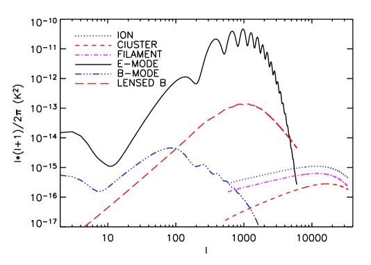
Figure 1: Polarisation power spectra for all ionized particles, filaments and cluster are shown by dotted, dot-dashed and short dashed curves, respectively. We also plot the primary $E$ mode induced by scalar perturbation (solid line), primary $B$ mode (triple dot-dashed line) from tensor mode and $B$ mode from lensed $E$ mode (long dashed line).

References

References

- [1] Couchnman H. M. P., Thomas P. A., Pearce F. R.,ApJ 452, 797 (1995)
- [2] Hu, W., ApJ 529, 12 (2000)
- [3] Kamionkowski M., & Loeb A., Phys. Rev. D 56, 5411 (1997)
- [4] Liu, G., et al, 2001, ApJ 561, 504 (2001)
- [5] Liu, G., da Silva, A., Aghanim, N. in preparation
- [6] Pearce F. R., & Couchnman H. M. P., New Astronomy, 2, 411(1997)
- [7] Portsmouth, J., astro-ph/0402173
- [8] Sazonov, S. Y.; Sunyaev, R. A., MNRAS, 310, 765(1999)
- [9] Seljak U., Hirata, C. M., Phys. Rev. D 69, 043005 (2004)
- [10] Suntaev R. A., Zel’dovich Y. B., MNRAS, 190, 413(1980)
- [11] Zaldarriaga, M. & Seljak, U.,Phys. Rev. D 55, 1830 (1997)
- [12] Zaldarriaga M., Seljak U.,Phys. Rev. D 58, 023003 (1998)