Primordial quadrupole-induced polarisation from filamentary structures and galaxy clusters

Abstract

We present the first computation of the Cosmic Microwave Background (CMB) polarisation power spectrum from galaxy clusters and filaments using hydrodynamical simulations of large scale structure. We give the $E$ and $B$ mode power spectra of the CMB quadrupole induced polarisation between $\ell\sim 560$ and $20000$. We find that the contribution from warm ionised gas in filamentary structures dominates the polarised signal from galaxy clusters by more than one order of magnitude on large scales (below $\ell\sim 1000$) and by a factor of about two on small scales ($\ell~{}\hbox to0.0pt{$>$\hss}{\lower 4.30554pt\hbox{$\sim$}}10000$). We study the dependence of the power spectra with $\sigma_{8}$. Assuming the power spectra vary like $\sigma_{8}^{n}$ we find $n=3.2-4.0$ for filaments and $n=3.5-4.6$ for clusters.

1 Introduction

After the success of the extraction of cosmological information from the Cosmic Microwave Background (CMB) temperature anisotropies, much effort is now put towards building experiments for measuring the CMB polarised signal, which is about one order of magnitude smaller. There are many scientific goals of the CMB polarisation studies. These include determining the reionisation epoch from the large scale polarisation power spectrum, testing inflationary models by searching specific patterns due to the existence of the primordial gravitational waves, and improving the precision of cosmological parameters derived by CMB temperature anisotropies alone. Aiming at these objectives, the satellites WMAP (Kogut et al., 2003) and Planck (Yurchenko, 2002), Balloon-borne experiments like ARCHEOPS (http://www.archeops.org/), Boomerang (Montroy et al., 2003) and MAXIPOL (Johnson et al., 2003) and Ground-based instruments like AMiBA (Lo et al., 2001) and DASI (Leitch et al., 2002) have observed or will observe the polarised sky.

An important issue concerning the measurement of the primordial polarisation power spectrum is that it is not the only polarised source in the sky. In addition to the contamination from the so-called foregrounds such as galactic dust (Benoit et al., 2003), free-free and synchrotron emissions (de Oliveira-Costa et al., 2003), there are other sources of polarisation due to large scale structure (LSS) (reionisation (Ng & Ng, 1996), weak lensing (Zaldarriaga & Seljak, 1998), …). In particular, when the CMB photons pass through the hot ionised gas trapped in the potential wells of galaxy clusters a polarised signal is induced. The presence of the CMB temperature quadrupole induces a linear polarisation in the scattered radiation. Sunyaev and Zel’dovich (1980) were the first to estimate the level of such a polarisation induced by galaxy clusters. These authors pointed out that in addition to the primary CMB quadrupole there are two other sources of temperature quadrupole seen by a cluster: A quadrupole due to the transverse peculiar velocity of the cluster, and double scattering. Studying the induced CMB polarisation due to clusters can open a whole new window for cosmology. Sunyaev and Zel’dovich proposed to use the polarisation to estimate cluster’s transverse velocity. Audit & Simmons (1999) gave a description of the effect due to the kinetic quadrupole, including the frequency dependence. Moreover, measuring the polarisation towards distant clusters should in principle permit to provide to observe the evolution of the CMB quadrupole. The CMB quadrupole seen by clusters contains statistical information on the last scattering surface at the cluster position. Therefore, measuring the cluster polarisation should help us to beat the cosmic variance (Kamionkowski & Loeb, 1997; Portsmouth, 2004). Sazonov & Sunyaev (1999) revisited the detailed polarisation signal due to the three sources of quadrupole given the constraint on the CMB quadrupole by COBE (Bennett et al., 1996), the electron density profiles of clusters and their transverse peculiar velocities. For the COBE data, their sky-average polarisation induced by the primordial quadrupole was found to be $3.1\tau\mu{\rm K}$, with $\tau$ the cluster optical depth. Additionally, if clusters possess an intra-cluster magnetic field, Faraday rotation will affect the linearly polarised CMB. This effect was investigated by Takada et al. (2001) who found an amplitude of the order of the microgauss at low frequencies. Inversely, the effect of Faraday rotation on the CMB polarisation was proposed to extract the information of the cluster magnetic field when the cluster electron density is obtained from SZ and X-ray observations (Ohno et al., 2002).

In this paper we concentrate on the case where no magnetic field is present in the intra-cluster gas. We study the polarised signal due to LSS by calculating the polarised angular power spectrum. Several authors have done some research in the polarisation due to ionised gas in clusters or at the reionisation. Hu (2000) investigated the secondary polarisation induced by several physical processes using an analytic method. For the polarisation in galaxy clusters, the author considered a density modulation of the kinetic and primordial polarisation sources similar to the Vishniac effect (Vishniac, 1987). Liu et al. (2001) computed the polarised signal at reionisation using N-body simulations in combination with an analytic description to model the gas distribution. More recently, Santos et al. (2003) investigated analytically the contribution from ionised patches at reionisation. They assumed the ionising sources reside in the dark matter halos and used the dark matter correlations in linear approximation. Both latter papers deal with the a polarisation induced by the primordial CMB quadrupole since it typically dominate over the kinetic and double scattering contribution at scales of interest. Concerning galaxy clusters, Baumann et al. (2003) computed the polarisation induced by primordial and kinetic quadrupole using a halo-clustering approach to describe fluctuations in the electron density. Lavaux et al. (2004) focus on the polarised signal due to the kinetic quadrupole and the double scattering by the use of hydrodynamical simulations.

In the present work, we revisit the polarisation signal induced by large scale structure. We use the analytical method developed in Liu et al. (2001) combined for the first time with state-of-the-art hydrodynamical simulation techniques. We concentrate on the the primordial CMB quadrupole induced polarisation as it is the dominant source. Hydrodynamical simulations are the most powerful tool to describe the physics of the gas. Taking advantage of this, we investigate the contribution to the polarised signal of different gas phases, namely the hot gas in galaxy clusters and the warm gas in filaments. In Section 2 and 3 we describe the method and the hydrodynamical simulations we used for our estimate. In Section 4, we present the results of our work and give a discussion and conclusion in Section 5 and 6 respectively.

Throughout this paper we will assume a flat $\Lambda$CDM cosmology with cosmological parameters matching present observations: matter density, $\Omega_{{\rm m}}=0.3$, cosmological constant density, $\Omega_{\Lambda}=0.7$, baryon density, $\Omega_{\rm b}=0.044$, and Hubble parameter, $h=0.71$.

2 Background

2.1 Analytic formulae

The polarised CMB signal is usually described by two of the Stokes parameters ${\cal Q}$ and ${\cal U}$. If we consider a wave traveling in the $\hat{z}$ direction, ${\cal Q}$ is the difference in intensity in the $\hat{y}$ and $\hat{x}$ directions, while ${\cal U}$ is the difference in the $(\hat{x}+\hat{y})/\sqrt{2}$ and $(\hat{x}-\hat{y})/\sqrt{2}$ directions. The circular polarisation parameter, ${\cal V}$, cannot be produced by scattering, so we will not mention it further. Polarisation calculations are more complicated than temperature calculations because the values for ${\cal Q}$ and ${\cal U}$ depend on the choice of coordinate system. Therefore, it is more convenient to decompose the polarisation on the sky into a divergence free component, the so-called $E$ mode, and a curl component, the so-called $B$ mode, which are coordinate independent.

We are interested in computing the $E$ and $B$ mode polarisation power spectra due to galaxy clusters and filaments. For this, we use the analytic formulae detailed in Liu et al. (2001) to which we refer the reader. In this work, the electron density fluctuation modulated quadrupole at any given scale ${\bf k}$ and conformal time $\eta$ is

$$S^{(m)}({\bf k},\eta) \equiv \int{\rm d}^{3}{\bf p}\delta_{\rm e}({\bf k-p},\eta)\Delta_{T2}^{(m)}({\bf p},\eta)$$ (1)

$$\simeq \delta_{\rm e}({\bf k},\eta)\int{\rm d}^{3}{\bf p}\Delta_{T2}^{(m)}({\bf p},\eta)$$

$$\equiv \delta_{\rm e}({\bf k},\eta)Q^{(m)}_{2}(\eta),$$

where $\delta_{e}$ is the electron density fluctuation, $\Delta_{T2}^{(m)}$ is the primordial CMB quadrupole with angular momentum $m=0,\pm 1,\pm 2$ and $Q^{(m)}_{2}(\eta)\equiv\int{\rm d}^{3}{\bf p}\Delta^{(m)}_{T2}({\bf p},\eta)$. The approximation in the second line assumes that the first order temperature quadrupole $\Delta^{(m)}_{T2}$ is uncorrelated with $\delta_{\rm e}$. In other words, the dominant contributions to the modulated quadrupole come mainly from the CMB quadrupole at large scales and from the electron density fluctuations at small scales, see Hu (2000). The temperature anisotropy field produced by scalar mode perturbations has axial symmetry. Therefore, the quadrupole field is decomposed into the $m=0$ component in the ${\bf p}$-basis parallel to the axis of symmetry, i.e. the temperature anisotropy quadrupole is $\Delta^{(0)}_{T2}Y_{2}^{0}(\beta,\alpha)$, where $\beta$ and $\alpha$ are the polar and azimuthal angles defining ${\bf\hat{n}}$ in this basis. Using the addition theorem, we can project the component in the ${\bf p}$-basis onto the ${\bf k}$- basis (see Ng & Liu 1999),

$$\sum_{m}Y^{m*}_{\ell}({\bf\hat{n}})Y_{\ell}^{m}({\bf\hat{p}})=\sqrt{\frac{2\ell+1}{4\pi}}Y_{\ell}^{0}(\beta,\alpha).$$ (2)

It then follows that

$$Q^{(m)}(\eta)=\sqrt{\frac{4\pi}{5}}\int{\rm d}^{3}{\bf p}\Delta^{(0)}_{T2}({\bf p},\eta)Y_{2}^{m*}(\hat{\bf p}).$$ (3)

Provided the modulated quadrupole $S$ Eq. (1), the polarised power spectrum can be obtained by integrating the Boltzmann equation along the photon past light cone. Here we skip the detailed derivation given in Liu et al., the power spectra for the $E$ and $B$ modes are:

$$C_{(E,B)\ell}=(4\pi)^{2}\frac{9}{16}\frac{(\ell+2)!}{(\ell-2)!}\sum_{m}\int k^{2}{\rm d}k\left\langle\left|\int{\rm d}\eta g(\eta)S^{(m)}({\bf k},\eta)T_{(E,B)\ell}^{(m)}(kr)\right|^{2}\right\rangle.$$ (4)

In this expression the first term is the visibility function $g(\eta)$, which is the probability that a photon had its last scattering at epoch $\eta$ and reaches the observer at the present time, $\eta_{0}$. It is defined as

$$g(\eta)\equiv-\frac{{\rm d}\tau}{{\rm d}\eta}{\rm e}^{\tau(\eta_{0})-\tau(\eta)},$$ (5)

where $\tau(\eta)\equiv\int_{\eta}^{\eta_{0}}d\eta^{\prime}an_{\rm e}\sigma_{\rm T}$ is the Thomson electron-scattering optical depth at time $\eta$. $S^{(m)}$ represents the source term of polarisation in Eq. (4). The last quantity is a geometrical factor $T_{(E,B)\ell}^{(m)}(kr)$ with $r=c(\eta_{0}-\eta)$ and $c$ the speed of light. It is given by the combination of the spherical Bessel functions. We list the results of $T_{(E,B)\ell}^{(m)}(kr)$ in Table 1. Note that the expression $T_{(E,B)\ell}^{(m)}(kr)$ in the Table are valid only in flat universes. The hyperspherical Bessel functions should be used in curved universe (Hu et al., 1998).

$m$	$T_{E\ell}^{(m)}$	$T_{B\ell}^{(m)}$
$0$	$(-i)^{\ell}\frac{j_{\ell}(kr)}{(kr)^{2}}$	0
$\pm 1$	$\mp(-i)^{\ell}\frac{1}{(2\ell+1)kr}\sqrt{\frac{1}{6\ell(\ell+1)}}[\ell j_{\ell}(kr)-(\ell+1)j_{\ell-1}(kr)]$	$\pm\sqrt{\frac{3(-i)^{\ell}}{2\ell(\ell+1)}}\frac{j_{\ell}(kr)}{(kr)^{2}}$
$\pm 2$	$\pm\frac{(-i)^{\ell}}{2\ell+1}\sqrt{\frac{(\ell-2)!}{6(\ell+2)!}}\left(\left[\frac{(\ell+2)(\ell+1)}{2\ell-1}+\frac{\ell(\ell+1)}{2\ell+3}+6\frac{(2\ell+1)(\ell-1)(\ell+2)}{(2\ell-1)(2\ell+3)}\right]\right.$	$\mp\frac{(-i)^{\ell}}{2\ell+1}\sqrt{\frac{(\ell-2)!}{6(\ell+2)!}}\left[(\ell+2)j_{\ell-1}(kr)\right.$
	$\left.\times j_{\ell}(kr)-(\ell+2)(\ell+1)\frac{j_{\ell-1}(kr)}{kr}-\ell(\ell-1)\frac{j_{\ell+1}(kr)}{kr}\right)$	$\left.-(\ell-1)j_{\ell+1}(kr)\right]$

Table 1: Contributions to the geometrical factor $T_{(E,B)\ell}^{(m)}$ for different $m$’s used in equation (4).

2.2 Simulation details

From Eq. (4) we easily see that the polarisation amplitude depends on the density of the electrons which scatter the CMB photons through $g(\eta)$ and $S^{(m)}$. We therefore expect that different gas phases contribute differently to the overall signal. One important step of our study is thus to quantify these contributions, using hydrodynamical N–body simulations to model the gas dynamics.

The simulations were generated with the public version of the Hydra code (Couchnman, Thomas, & Pearce 1995;Pearce & Couchman 1997), which implements an adaptive particle-particle/particle-mesh (AP³M) algorithm (Couchman, 1991) to calculate gravitational forces and smoothed particle hydrodynamics (SPH) (Monaghan, 1992) to estimate hydrodynamical quantities. In the present study, we consider a non-radiative model, i.e. the gas component evolves under the action of gravity, viscous forces and adiabatic expansion. The effects of non-gravitational heating and radiative dissipation of energy, will be addressed in a subsequent study.

We present results from three simulation runs of the $\Lambda$CDM cosmology adopted in this paper (see Section 1). The initial density and velocity fields were constructed with $160^{3}$ particles of both baryonic and dark matter, perturbed from a regular grid of fixed comoving size $L=100h^{-1}{\rm Mpc}$, using the Zel’dovich approximation. With this choice of parameters the mass of each baryonic and dark matter particles were $m_{\rm gas}=2.6\times 10^{9}\,h^{-1}M_{\odot}$ and $m_{{\rm dark}}=2.1\times 10^{10}\,h^{-1}M_{\odot}$, respectively. We assumed a matter power spectrum described by the CDM transfer function in Bardeen et al. (1986) (known as the BBKS transfer function for CDM models) with shape parameter, $\Gamma$, given by the formula in Sugiyama (1995). The normalisation of the matter power spectrum in each simulation run was set such that the present day r.m.s matter fluctuations in spheres of $8h^{-1}$ Mpc radius, $\sigma_{8}$, was equal to 0.8, 0.9 and 1 respectively. We used the same realisation of the power spectrum in each run to permit direct comparison between forming structures in the three simulations. The runs were started at redshift $z=49$. The gravitational softening was fixed at $25\,h^{-1}{\rm kpc}$ in physical units between redshifts zero and one, and held constant above this redshift to $50\,h^{-1}{\rm kpc}$ in comoving coordinates.

3 Method

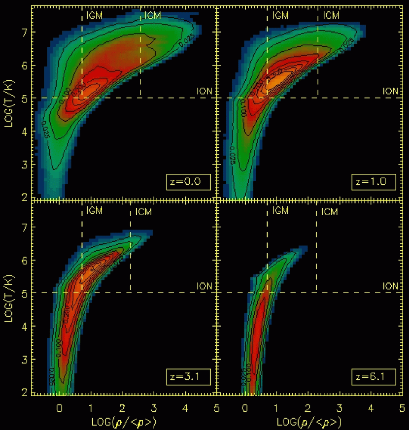
Figure 1: Temperature-overdensity distribution (phase-space) of gas particles in the $\sigma_{8}=0.9$ simulation at redshifts z=0, 1, 3.1, and 6.1 (top right, top left, bottom left and bottom right panels, respectively). In each panel, horizontal dashed lines represent the temperature threshold, $T_{\rm th}$, above which the gas is considered to be ionised. The ICM and IGM phases are defined in each panel by the vertical dashed lines.

We study the relative contribution to the polarisation power spectrum from clusters (hot high-density gas) and filamentary structures (warm low-density gas). We define the gas phases based on the baryon collapsed density and temperature. We call hot ionised gas the phase consisting of all gas particles with temperatures above the threshold $T_{\rm th}=10^{5}$ K. Gas above this temperature threshold is assumed fully ionised and is considered in the calculations as the only gas scattering the CMB photons. Hot ionised gas particles with overdensities, $\delta_{i}$, larger than the density contrast at collapse, $\Delta_{c}=178\Omega_{m}(z)^{-0.55}$ (Eke, Navarro, & Frenk 1998), are turn considered to be part of the intra cluster medium (ICM) high-density phase. Low-density ionised gas particles with overdensities ranging in the interval $5<\delta_{i}<\Delta_{c}$ encompass a warm intergalactic medium (IGM) phase (see e.g. Valageas, Schaeffer, & Silk (2002)) which we call “filamentary structures”. Fig. (1) shows the overdensity-temperature distribution (phase space) of all gas particles in our $\sigma_{8}=0.9$ simulation run at redshifts $z=0$ (top left panel), $z=1$ (top right panel), $z=3.1$ (bottom left panel) and $z=6.1$ (bottom right panel). In each case the phase space was discretised in bins of size dex=0.1 per logarithmic decade, that gives the gas fraction density (gas fraction per dex²) in each bin. The horizontal dashed lines represent the temperature threshold, $T_{\rm th}$, above which the gas is considered to be ionised. The ICM and IGM phases are defined in each panel by the vertical dashed lines. We should note that our simulations do not include photoinisation heating due to UV background radiation, which explains the significant fraction of very cold low-overdensity gas. In our present simulations, resolution together with a simplified physical model prevent us from properly describing this gas phase.

In order to calculate the $E$ and $B$ power spectra using Eq. (4), we need to evaluate the electron density, $\delta_{\rm e}({\bf k},\eta)$, and the primordial CMB quadrupole, $\Delta_{T2}^{(m)}$ which appears in Eq (3). We modify the publicly available code CMBFast (Zaldarriaga & Seljak, 1997) to output the time evolution of the primordial CMB quadrupole at different ${\bf k}$ modes. This is then integrated in k-space at each epoch to obtain $Q^{(m)}_{2}(\eta)$ in Eq. (1). The next step is to compute the visibility function $g(\eta)$ and the polarisation source term Eq. (1) for which the electron density fluctuations $\delta_{\rm e}({\bf k},\eta)$, are needed. The first quantity is obtained directly from our simulation runs by evaluating the ionisation fraction at different redshifts. For the electron density fluctuations, we start by evaluating this in real space, $\delta_{\rm e}({\bf r},\eta)$, on a regular grid with $N_{\rm grid}^{3}$ cells inside the comoving box, making use of the SPH formalism (Monaghan, 1992). In this step we assume a primordial gas composition with 24% helium abundance. The computation of $\delta_{\rm e}({\bf k},\eta)$ follows by performing the Fourier transform of $\delta_{\rm e}({\bf r},\eta)$.

4 Power spectra of polarisation of clusters and filaments

We compute the $E$ and $B$ power spectra for filaments, galaxy clusters and all ionised gas. Results obtained adopting a regular grid with $600^{3}$ cells (corresponding to a fixed cell separation of $0.17\,h^{-1}{\rm Mpc}$ in comoving coordinates) are shown in Fig. (2) in the $\sigma_{8}=0.9$ case. We tested the convergence of our results by comparing $C_{(E,B)\ell}$ evaluated with $300^{3}$, $450^{3}$ and $600^{3}$ grids and found no significant difference between the last two values. This indicates we reached numerical convergence. The domain of validity of our results is $560~{}\hbox to0.0pt{$<$\hss}{\lower 4.30554pt\hbox{$\sim$}}\ell~{}\hbox to0.0pt{$<$\hss}{\lower 4.30554pt\hbox{$\sim$}}20000$, outside which we reach numerical resolution limits. We also tested for the temperature threshold. Lowering $T_{\rm th}$ to $10^{4}$K, decreases the power spectra by no more than 20%.

We note that we get the same power for the secondary $E$ and $B$ mode polarisation with a maximum relative difference smaller than $10^{-6}$. The reason for this equality is essentially that the first-order quadrupole, whose scattering produces the polarisation, is dominated by large scales and has thus a random orientation relative to the small-scale electron density fluctuations. Scattering of the quadrupole by the small-scale fluctuations therefore, on average, excites $E$ and $B$ modes equally (e.g. Hu 2000, Liu et al. 2001).

We now compare the contributions to the polarisation signal from clusters and filaments, the dotted and the long dashed lines, respectively, in Fig. (2). For the filaments, the shape of the power spectrum is very similar to that induced by all ionised particles, but the amplitude is smaller by a factor of about $1.7$. On large scales ($\ell\sim 1000$) the power spectrum of filaments dominates that of clusters by one order of magnitude. On small scales ($\ell\sim 17000$), this difference is only a factor of two indicating that clusters contribute mainly at large $\ell$’s, as expected.

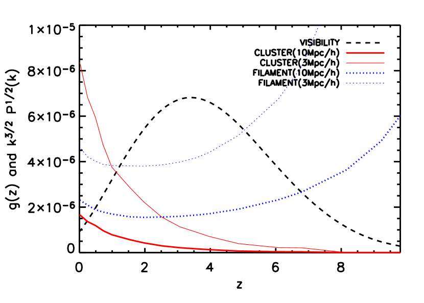
Figure 3: Visibility function (dashed line) and square root of the logarithmic power for the clusters and filaments phases at two characteristic scales (3 and 10 $h^{-1}$Mpc). Results are displayed using an arbitrary normalisation factor for the power.

We illustrate the difference between cluster and filament polarised power spectra by plotting in Fig. (3) the evolution of the visibility function (thick dashed line) and density perturbations at two typical scales 3 and 10 $h^{-1}{\rm Mpc}$ for clusters and filaments, respectively. Recall the Eq. (4), the power spectrum is the integral of the electron density weighted by the visibility function. At the typical cluster scale, the power does not exceed that of filaments, down to $z\sim 1$. At that redshift, the visibility function from our simulation is relatively small. It peaks at $z~{}\hbox to0.0pt{$>$\hss}{\lower 4.30554pt\hbox{$\sim$}}3.2$ and its full width half maximum is bounded by $z\sim 1.1$ and $z\sim 6.2$. In this range of redshifts, the power from filaments is much larger than from clusters. As a consequence, most of the scattering producing the linear polarisation occurs for $z~{}\hbox to0.0pt{$>$\hss}{\lower 4.30554pt\hbox{$\sim$}}1.2$ when the relative contribution of clusters is still small.

The power spectrum of polarisation induced by total ionised particles (solid curve in Fig (2)), peaks at a scale of about $\ell\sim 10000$ with an amplitude much smaller than the primary $E$ mode polarisation. We now compare the power spectrum of the secondary polarisation and the power spectrum of the secondary temperature anisotropies due to SZ effect for the all ionised phase. We base our comparison on the results of da Silva et al. (da Silva et al., 2001). They have estimated the SZ temperature power spectrum using similar non-radiative simulations. The amplitude of the SZ temperature power spectrum is five orders of magnitudes larger than the polarisation signal (see Fig. 3 in da Silva et al. (2001)). In Fig. 4 of da Silva et al. (2001), the power spectrum of temperature anisotropies associated with clusters, in the non-radiative case, dominates by almost a factor 2 that of filaments whereas the power spectrum of polarised signal is dominated by filaments. This is because the amplitude of the SZ temperature anisotropy is an integral of the free electron density weighted by the gas temperature. Typically, the temperature in clusters is one hundred times higher than the temperature in filaments. The secondary polarisation signal, although weak, can provide complementary information to that we get from secondary temperature fluctuations especially for the filaments.

5 Discussion

This is the first time we are able to investigate simultaneously the polarisation contribution from ICM and IGM gas phases using hydrodynamical simulations. Therefore direct comparisons with previous studies, based either on analytic computations or on N-body simulations, are not straightforward especially for the filamentary structures but also for clusters. As an example, our angular power spectrum for cluster matches the one given by Santos et al. (2003) particularly below $\ell\sim 1000$. However they consider, in their halo model, structures within $100<T_{vir}<10^{4}$K which we do not model here (see Sec. 2.2). Our results from the ICM phase are easier to compare by nature with those from Liu et al. (2001), which are based on N-body computations. Our polarisation power spectrum for clusters is in very good agreement with the relevant models, namely A and B, in Fig. 4 of Liu et al. Finally, we find that the amplitude of the power spectrum induced by galaxy clusters, at its maximum, is consistent with the estimate of Sazonov & Sunyaev  (1999) for the sky-averaged polarisation: $3.1\tau\mu{\rm K}\sim 30\ {\rm nK}$, with a typical optical depth for clusters $\tau=0.01$. From our hydro-dynamical simulation we find an average value of 24 nK.

As suggested by Eq. (4), the amplitude of the secondary polarised signal from clusters is expected to have a strong dependence on the amplitude of the density fluctuations, which is usually parameterised by $\sigma_{8}$. To estimate the effect of $\sigma_{8}$ on our results, we compare in Fig. (4) the power spectra obtained with the three simulations: $\sigma_{8}=0.8$ (long-dashed line), 0.9 (solid line) and 1 (dashed line). Panel (a) shows the total power spectrum from all ionised particles. Panels (b) and (c) exhibit the power from the IGM and ICM respectively. Assuming the power spectra from clusters, filaments and all ionised particles vary like $C_{E,Bl}\propto\sigma_{8}^{n}$ we get $n=3.0-4.4$ for all ionised particles, $3.2-4.0$ for filaments and $3.5-4.6$ for clusters. The amplitude of the polarisation power spectrum is sensitive with $\sigma_{8}$, however, the value of the index $n$ is smaller than that obtained for the SZ power spectrum variation $6~{}\hbox to0.0pt{$<$\hss}{\lower 4.30554pt\hbox{$\sim$}}n~{}\hbox to0.0pt{$<$\hss}{\lower 4.30554pt\hbox{$\sim$}}9$ (see for example Zhang, Pen, & Wang (2002), Bond et al. (2002), Komatsu & Seljak (2002))

We compare our secondary polarisation spectra (solid, dotted and long-dashed lines in Fig. (2)) with the primary $E$ and $B$ modes sue to scalar and tensor mode perturbations (dashed and dot-dashed lines respectively). The $E$ mode signal from clusters and filaments dominates the primary signal at $\ell~{}\hbox to0.0pt{$>$\hss}{\lower 4.30554pt\hbox{$\sim$}}5000$. Below this scale, the secondary polarised signal is always very small and therefore do not significantly contaminate the primary signal. Gravitational waves, i.e. tensor mode perturbations, induce primary $B$ mode polarisation which amplitude depends on the ratio of tensor to scalar quadrupole, $r=C^{T}_{\ell}/C^{S}_{\ell}$, which is not well constrained at present. We compute the primary $B$ mode signal, with $0<r<0.9$ within the upper limits (at $95\%$ confidence level) set by WMAP+CBI+ACBAR+2dFGRS+Lyman$\alpha$ (Spergel, 2003) observations and the tensor spectral index $n_{t}=-r/8$, and compare it with our secondary $B$ mode signal. We conclude that within $0<r<0.9$ the secondary signal does not prevent us from detecting gravitational wave induced polarisation at scales $\ell~{}\hbox to0.0pt{$<$\hss}{\lower 4.30554pt\hbox{$\sim$}}100$.

Gravitational lensing by large scale structures modifies slightly the primary $E$ mode power spectrum. Most noticeably it generates, through mode coupling, $B$ mode polarisation out of pure $E$ mode signal (Benabed, Bernardeau, & van Waerbeke 2001;Zaldarriaga & Seljak 1998). The gravitational lensing-induced signal, which peaks around $\ell\sim 1000$, is a major issue for primary $B$ mode measurement. We compare in Fig. (2) the $B$ mode power spectrum of the polarised signal from gravitational lensing by large scale structures to that associated with clusters and filaments. We find the latter is about two orders of magnitude smaller and it dominates at very small angular scales ($\ell~{}\hbox to0.0pt{$>$\hss}{\lower 4.30554pt\hbox{$\sim$}}10000$). The polarised signal from clusters and filaments might be observed at larger angular scales if the lensing-induced $B$ modes can be significantly cleaned by appropriate techniques as those proposed for example by Seljak & Hirata (2004). We note that the dependence of lensing-induced polarisation on $\sigma_{8}$ is different from that of clusters and filaments. An increase of $\sigma_{8}$ would enhance more the latter with respect to the former.

6 Conclusion

In this paper, we present the first computation of the $E$ and $B$ mode quadrupole-induced polarisation power spectra of galaxy clusters and filaments using hydrodynamical LSS simulations.

We find that the power spectrum from filaments dominates the power from clusters by a factor of about two on small scales, and by one order of magnitude on large scales. The secondary polarisation signal can thus provide complementary information to those we get from secondary temperature fluctuations especially for filaments. Assuming the power spectra vary like $\sigma_{8}^{n}$ we find $n$ in the range 3 to 4.6 depending on the gas phase.

As expected, the secondary polarisation power spectra dominate at small angular scales. Although this first computation of the polarisation from filaments shows that the signal can be one order of magnitude larger on large scales, the secondary polarisation is still subdominant. Therefore it is not a major problem for the primordial $B$ mode detection.

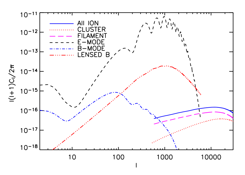
Figure 2: Polarisation power spectra for $\sigma_{8}=0.9$. The polarisation power spectra for all ionised particles, filaments and clusters are shown by solid, long-dashed and doted curves, respectively. We also plot the primary $E$ mode induced by scalar perturbations (short-dashed line), primary $B$ mode (dot-dashed line) from tensor perturbations and $B$ mode from lensed $E$ mode (dot-dot-dashed line).

Figure 4: Power spectra of secondary polarisation from simulations with different $\sigma_{8}$. Panel (a) is for all ionised particles, panel (b) and (c) are for filaments and clusters respectively.

References

- Audit & Simmons (1999) Audit, E., & Simmons, J. F. L. 1999 MNRAS., 305, 27
- Bardeen et al. (1986) Bardeen, J. M., Bond, J. R., Kaiser, N., & Szalay, A. S., 1986, ApJ, 304, 15
- Baumann, Cooray, & Kamionkowski (2003) Baumann, D., Cooray, A., & Kamionkowski, M., 2003, New Astron., 8, 565
- Benabed, Bernardeau, & van Waerbeke (2001) Benabed, K., Bernardeau, F., & van Waerbeke, L., 2001, Phys.Rev. D63, 043501
- Bennett et al. (1996) Bennett, C. L., et al., 1996, ApJ, 462, L49
- Benoit et al. (2003) Benoit, A., et al., astro-ph/0306222
- Bond et al. (2002) Bond, J. R., et al. 2002, ApJsubmitted, astro-ph/0205386
- Cooray & Sheth (2002) Cooray, A., & Sheth, R., 2002, Phys.Rept. 372, 1
- Couchman (1991) Couchman, H. M. P., 1991, Ap.J, 368, L23
- Couchnman, Thomas, & Pearce (1995) Couchnman, H. M. P., Thomas, P. A., Pearce, F. R., 1995, ApJ, 452, 797
- da Silva et al. (2001) da Silva, A., et al., 2001, ApJ, 561L, 15D
- Eke, Navarro, & Frenk (1998) Eke, V. R., Navarro, J. F., & Frenk, C. S., 1998, ApJ, 503, 569
- Hu et al. (1998) Hu, W., Seljak, U., White, M., & Zaldarriaga, M., 1998, Phys. Rev. D, 57, 3290
- Hu (2000) Hu, W., 2000, ApJ, 529, 12
- Johnson et al. (2003) Johnson, B. R. et al., 2003, New Astronomy Reviews, 47, 1067J
- Kamionkowski & Loeb (1997) Kamionkowski, M., & Loeb, A., 1997, Phys. Rev. D, 56, 5411
- Kogut et al. (2003) Kogut, A. et al, 2003, Astrophys.J.Suppl. 148, 161
- Komatsu & Seljak (2002) Komatsu, E., & Seljak U., 2002, MNRAS, 336, 1256
- Lavaux et al. (2004) Lavaux, G., Diego, J. M., Mathis, H., & Silk, J. 2004, MNRAS. 347, 729
- Leitch et al. (2002) Leitch, E. M. et al., 2002, Nature 420, 763
- Liu et al. (2001) Liu, G. C., Sugiyama, N. Benson, A. J., Lacey, C. G., & Nusser, A., 2001, ApJ, 561, 504
- Lo et al. (2001) Lo, K., et al., 2001, AIPC., 586, 172L
- Monaghan (1992) Monaghan, J. J., 1992, Ann. Rev. Astron. Astrophys., 30, 543
- Montroy et al. (2003) Montroy, T. et al., 2003, New Astronomy Reviews, 47, 1057
- Ng & Liu (1999) Ng, K.-W., & Liu G.-C., 1999, Int. J. Mod. Phys. D8, 61-83
- Ng & Ng (1996) Ng, K. L., & Ng, K.-W., 1996, ApJ, 456, 413
- Ohno et al. (2002) Ohno, H., Takada, M., Dolag, K., Bartelmann, D., & Sugiyama, N, 2002, ApJ, 584, 599
- de Oliveira-Costa et al. (2003) de Oliveira-Costa, A., et al. 2003, Phys.Rev. D 68 083003
- Pearce & Couchman (1997) Pearce, F. R., & Couchnman, H. M. P., New Astronomy, 2, 411(1997)
- Portsmouth (2004) Portsmouth, J., astro-ph/0402173
- Santos et al. (2003) Santos, M. B., Cooray, A., Haiman, Z., Knox, L., & C.-P. Ma, 2003, ApJ, 598, 756
- Sazonov & Sunyaev (1999) Sazonov, S. Y., & Sunyaev, R. A., MNRAS, 310, 765(1999)
- Seljak & Hirata (2004) Seljak, U., & Hirata, C. M., 2004, Phys. Rev. D 69, 043005
- Spergel (2003) Spergel, D.N., et al., 2003, ApJS, 148, 175
- Sugiyama (1995) Sugiyama, N., 1995, Astrophys.J.Suppl. 100, 281
- Sunyaev & Zel’dovich (1980) Suntaev, R. A., & Zel’dovich, Y. B., 1980, MNRAS, 190, 413
- Takada, Ohno, & Sugiyama (2001) Takada, M., Ohno, H., & Sugiyama, N. astro-ph/0112412
- Valageas, Schaeffer, & Silk (2002) Valageas, P. Schaeffer, R., & Silk, J., 2001, Astron. Astrophys., 367, 1
- Vishniac (1987) Vishniac, E. T.,1987, ApJ, 322, 597
- Yurchenko (2002) Yurchenko, V., 2002, AIP Conf.Proc. 616, 234;
- Zaldarriaga & Seljak (1997) Zaldarriaga, M., & Seljak, U., 1997, Phys. Rev. D55, 1830
- Zaldarriaga & Seljak (1998) Zaldarriaga, M., & Seljak, U., 1998, Phys. Rev. D, 58, 023003
- Zhang, Pen, & Wang (2002) Zhang, P., Pen, U., & Wang, B., 2002, ApJ, 577, 555