Constraints on dark energy models from galaxy clusters with multiple arcs

Abstract

We make an exploratory study of how well dark energy models can be constrained using lensed arcs at different redshifts behind cluster lenses. Arcs trace the critical curves of clusters, and the growth of critical curves with source redshift is sensitive to the dark-energy equation of state. Using analytical models and numerically simulated clusters, we explore the key factors involved in using cluster arcs as a probe of dark energy. We quantify the sensitivity to lens mass, concentration and ellipticity with analytical models that include the effects of dark energy on halo structure. We show with simple examples how degeneracies between mass models and cosmography may be broken using arcs at multiple redshifts or additional constraints on the lens density profile. However we conclude that the requirements on the data are so stringent that it is very unlikely that robust constraints can be obtained from individual clusters. We argue that surveys of clusters, analyzed in conjunction with numerical simulations, are a more promising prospect for arc-cosmography.

We use such numerically simulated clusters to estimate how large a sample of clusters/arcs could provide interesting constraints on dark energy models. We focus on the scatter produced by differences in the mass distribution of individual clusters. We find from our sample of simulated clusters that at least 1000 pairs of arcs are needed to obtain constraints if the mass distribution of individual clusters is taken to be undetermined. We discuss several unsolved problems that need study to fully develop this method for precision studies with future surveys.

1 Introduction

The compelling observational evidence for an accelerating expansion of the universe has led to much recent work on models for dark energy that would drive this expansion (see PE02.2; PA03.1 and CA03.1 for reviews). Unless the dark energy is a cosmological constant, it is likely that it evolves with time. The best observational probes of dark energy are therefore ones that measure the geometry of the universe at different redshifts, allowing for a mapping of the evolution of dark energy. So far Type-Ia supernovae, which measure the luminosity distance over a range of redshifts, and the multipole orders of the acoustic peaks in the power spectrum of the cosmic microwave background, have been the only geometric probes of dark energy (PE99.1; RI98.1; SP03.1; see HU01.2 for a discussion of different probes).

The multiple imaging of background galaxies into arcs by foreground galaxy clusters has been used to probe the mass distribution of clusters. The position of the arcs on the sky depends on the mass enclosed within the lensing region of the cluster and also on ratios of angular diameter distances, which we will refer to as the geometric information probed by lensing. Observations of multiple arcs at different redshifts have been suggested as probes of dark energy (LI98.1; GO02.2; SE02.1). The idea is that the relative positions of arcs at different redshifts depend only weakly on the mass distribution and therefore probes the lensing geometry. Recently SO04.1 analysed Abell 2218 using arcs at four different redshifts to constrain dark energy models, obtaining $w\la-0.85$ at 68.3% confidence for constant $w$.

A critical issue in the reliability of geometric measurements from cluster lensing is the sensitivity of the results to the mass distribution of the cluster. If the cluster mass were smoothly distributed, then it is easy to see that multiple arcs are a good probe of geometry, but realistic clusters are likely to have substructure and ellipticity. Ideally one would like to be able to independently measure the mass distribution responsible for lensing, so that no theoretical assumptions need be made in inferring geometric information (e.g. CH02.2).

In this paper we use numerical simulations of lensing clusters to explore two approaches to constraining dark energy models with cluster arcs. The first may be called the “golden lens” approach: we ask how external information about the cluster mass distribution can allow dark energy constraints to be obtained from just one or a few lens systems. The second is a statistical approach: we ask how large a sample of clusters is needed to make an “ensemble averaged” measurement of critical curve versus redshift, which can then be compared to simulations. The two approaches seek different kinds of datasets, and the latter assumes that simulations (calibrated to some extent from the data) represent lensing clusters adequately well at least for the giant arcs.

We describe our parameterisation of dark energy models in Sect. 2. The lensing formalism is presented in Sect. 3, and the analytic dependence of critical curves on cosmology is shown. In Sect. 4, we extend the study to numerical cluster models, and we summarise in Sect. 5.

2 Dark-energy models

We work with the metric

$$ds^{2}\,=\,a^{2}\left[-(1+2\phi)d\tau^{2}\,+\,(1-2\phi)(d\chi^{2}+r^{2}d\Omega^{2})\right],$$ (1)

where we have used the comoving coordinate $\chi$ and $a(\tau)=(1+z)^{-1}$ is the scale factor as a function of conformal time $\tau$. We adopt units such that $c=1$. The comoving angular diameter distance $r(\chi)$ depends on the curvature: we assume a spatially flat universe so that $r(\chi)=\chi$. The density parameter $\Omega$ has contributions from mass density $\Omega_{\rm m}$ or dark energy density $\Omega_{\rm de}$, so that $\Omega=\Omega_{\rm m}+\Omega_{\rm de}$.

Dark energy models are often described in terms of the equation of state $p=w\rho$, with $w=-1$ corresponding to a cosmological constant. The time dependence of $w$ is commonly parameterised as $w=w_{0}+w_{a}(1-a)$ (LI03.1). For comparison with other work we will compare $w_{a}$ to $w^{\prime}$ defined by $w=w_{0}+w^{\prime}z$. The Hubble parameter $H(a)$ is given by

$$H(a)=H_{0}\left[\Omega_{m}a^{-3}+\Omega_{\rm de}e^{-3\int_{1}^{a}d\ln a^{\prime}(1+w(a^{\prime}))}\right]^{1/2},$$ (2)

where $H_{0}$ is the Hubble parameter today. The comoving distance $\chi(a)$ is

$$\chi(a)=\int_{1}^{a}\frac{da^{\prime}}{a^{\prime 2}H(a^{\prime})},$$ (3)

The above equation shows how the lensing observables depend on integrals over the dark-energy dependent expansion rate.

We consider four different cosmological models in this study (see Table 1 and DO03.2 for details). These can be described in terms of an effective values of $w_{0}$ and $w_{a}$. One is the standard cosmological-constant model with flat geometry and $\Omega_{\Lambda}=0.7$. The second has a constant ratio $w_{0}=-0.6$ between pressure and energy density of the dark energy (DECDM). The remaining two use different descriptions for the self-interaction potential of the dark-energy scalar field. One has a power-law potential (Ratra-Peebles, RP; see PE02.2), the other has a power-law potential multiplied by an exponential (SUGRA; BR00.2). The RP and SUGRA models have the same values of $w$ at the present time, $w_{0}\simeq 0.8$, but very different evolution histories. See DO03.2 for other details of the models and their implementation in the simulations used here.

Table 1: Parameters characterising the cosmological models

Model	$\Omega_{\rm m}$	$\Omega_{\rm dm}$	$H_{0}/100$	$\sigma_{8}$	$w_{0}$	$w_{a}$
$\Lambda$CDM	0.3	0.7	0.7	0.9	-1	0
DECDM	0.3	0.7	0.7	0.9	-0.6	0
RP	0.3	0.7	0.7	0.9	-0.83	0.1
SUGRA	0.3	0.7	0.7	0.9	-0.83	0.5

3 Analytic models

3.1 General properties

We adopt the density profile proposed by NA97.1 (hereafter NFW) for modelling cluster lenses, which was found to fit numerically simulated galaxy clusters well. We investigate here how strong lensing by analytical NFW halos changes when the dark-energy equation of state is changed, and postpone effects of the substructure and asymmetry of realistic halos to Sect. 5. The profile is given by

$$\rho(r)=\frac{\rho_{\mathrm{s}}}{(r/r_{\mathrm{s}})(1+r/r_{\mathrm{s}})^{2}}\;,$$ (4)

where $\rho_{\mathrm{s}}$ and $r_{\mathrm{s}}$ are characteristic density and distance scales, respectively. These two parameters are strongly correlated (NA97.1).

The concentration is defined as $c=r_{200}/r_{\mathrm{s}}$, where $r_{200}$ encloses a mean halo density of $200$ times the critical cosmic density. Numerical simulations show that $c$ depends on the virial mass $M$ of the halo, which can thus be used as the only free parameter. Several algorithms have been developed for relating $c$ to $M$. In this work, we adopt that proposed by EK01.1 because, as recently demonstrated by DO03.2, it performs very well also in dark-energy cosmologies. The concentration also depends on the cosmological model, implying that the lensing properties of haloes with identical mass are different in different cosmological models if they are modelled with the NFW profile. This is an important difference of our work to earlier studies (LI98.1; GO02.2; SE02.1).

The lensing properties of the NFW profile have been widely investigated in the past (see e.g. BA96.1; WR00.1; LI02.1; PE02.1; ME03.1), thus we summarise them only briefly. Lensing is fully described by the lensing potential $\psi$. For axially symmetric models, computing the lensing potential reduces to a one-dimensional problem. We define the optical axis as the straight line passing through the observer and the lens centre and introduce the physical distances perpendicular to the optical axis on the lens and source planes, $\xi$ and $\eta$, respectively. We then choose $r_{\mathrm{s}}$ as a length scale in the lens plane and define the dimensionless distance $x\equiv\xi/r_{\mathrm{s}}$ from the lens centre. By projecting $r_{\mathrm{s}}$ to the source distance, we define a corresponding dimensionless distance $y\equiv(\eta/r_{\mathrm{s}})(D_{\mathrm{l}}/D_{\mathrm{s}})$ from the optical axis in the source plane.

Defining $\kappa_{\mathrm{s}}\equiv\rho_{\mathrm{s}}r_{\mathrm{s}}\Sigma_{\mathrm{cr}}^{-1}$, where $\Sigma_{\mathrm{cr}}=[c^{2}/(4\pi G)]\,[D_{\mathrm{s}}/(D_{\mathrm{l}}D_{\mathrm{ls}})]$ is the critical surface mass density for strong lensing and $D_{\mathrm{ls}}$ is the angular diameter distance between the lens and the source planes, the lensing potential can be written as

$$\psi(x)=4\kappa_{\rm s}g(x)\>,$$ (5)

where

$$g(x)=\frac{1}{2}\ln^{2}\frac{x}{2}+\left\{\begin{array}[]{l@{\quad\quad}l}2\,\mbox{arctan}^{2}\sqrt{\frac{x-1}{x+1}}&(x>1)\\ -2\,\mbox{arctanh}^{2}\sqrt{\frac{1-x}{1+x}}&(x<1)\\ 0&(x=1)\end{array}\right.\;.$$ (6)

Axially symmetric models are generally inappropriate for describing lensing by galaxy clusters (ME03.1) because their typically high degree of asymmetry and substructure changes their lensing properties qualitatively and substantially. The tidal (shear) field produced by an asymmetric mass distribution can be partially mimicked by including ellipticity into the model. We adopt the model proposed by ME03.1, who obtained an elliptical generalisation of the NFW axially symmetric lensing potential by substituting in Eq. (5)

$$x\rightarrow x^{\prime}=\sqrt{\frac{x_{1}^{2}}{(1-e)}+x_{2}^{2}(1-e)}\;,$$ (7)

where $x_{1}$ and $x_{2}$ are the two Cartesian components of $x$, $x^{2}=x_{1}^{2}+x_{2}^{2}$. We define the ellipticity as $e\equiv 1-b/a$, where $a$ and $b$ are the major and minor axes of the ellipse, respectively.

The lensing potential implies the Jacobian matrix of the lens mapping,

$$A\equiv\left(\delta_{ij}-\frac{\partial^{2}\psi(\vec{x})}{\partial x_{i}\partial x_{j}}\right)\ ,$$ (8)

whose determinant vanishes on the critical curves of the lens. In particular, the tangential critical curve is located where the tangential eigenvalue of the Jacobian matrix vanishes,

$$\lambda_{\rm t}=1-\kappa-\gamma=0\;,$$ (9)

where $\kappa$ and $\gamma=(\gamma_{1},\gamma_{2})$ are the lens convergence and shear, respectively. They can be written in terms of the lensing potential as

$$\kappa(\vec{x})=\frac{1}{2}(\psi_{11}+\psi_{22})$$ (10)

and

$$\gamma_{1}(\vec{x}) = \frac{1}{2}(\psi_{11}-\psi_{22})$$ (11)

$$\gamma_{2}(\vec{x}) = \psi_{12}=\psi_{21}\ ,$$ (12)

where we abbreviate

$$\frac{\partial^{2}\psi(\vec{x})}{\partial x_{i}\partial x_{j}}\equiv\psi_{ij}\ .$$ (13)

3.2 Sizes of critical curves and cosmology

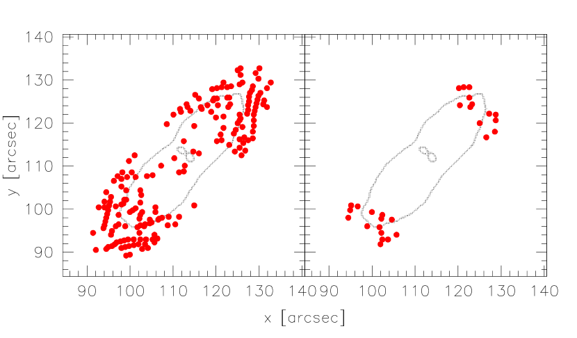
Figure 1: Position of gravitational arcs with length-to-width ratio larger than 5 (left panel) and 10 (right panel) in a lensing simulation; also shown are the critical curves of the lensing cluster.

Tangential arcs form near the tangential critical curves of a lensing cluster. We assume in the following that there is a correspondence between the tangential critical curves and the observed position of tangential arcs. In practice, tangential arcs with moderate length-to-width ratio may form quite far from tangential critical curves if the cluster is embedded into a strong shear field. To reduce this uncertainty, arcs with a large tangential-to-radial magnification ratio must be used.

The problem is illustrated in Fig. 1, where we show the position of all images with length-to-width ratio $\geq 5$ (left panel) and $\geq 10$ (right panel), found in a ray-tracing simulation using a numerical cluster model as a lens. A large number of elliptical sources were distributed in the region containing the lens caustics in order to obtain a large number of arcs. In this particular case, the tangential critical curve appears very elongated, showing that the cluster mass distribution is far from axially symmetric. From the first panel it is clear that arcs with substantial tangential distortion form in a wide region surrounding the critical curves. For example, using arcs with a length-to-width ratio $\geq 5$, the spread in arc positions is $\sim 10^{\prime\prime}$; selecting arcs with high length-to-width ratio ($\geq 10$) reduces the spread to a few arc seconds.

It is important to note that arcs with large length-to-width ratios form along those portions of the critical curves which are at the largest distances from the cluster centre. In comparing theory to observations, one possibility is to compare in detail the arcs in a simulated sample with observed arcs. However to avoid the computational expense of lensing source galaxies through the numerical clusters discussed in the next section, we will use an average size of the critical curve weighted with the inverse radial magnification as a proxy for the location of large arcs. Hence we do the same here by assigning to the $i$-th point on the tangential critical curve a weight:

$$p_{i}=|2[1-\kappa(\vec{x}_{i})]|\;.$$ (14)

The size of the critical curve is then measured as the weighted average distance of the critical points from the lens centre,

$$x_{\rm c}=\frac{\sum_{i}p_{i}|\vec{x}_{i}|}{\sum_{i}p_{i}}\;.$$ (15)

The weight factor that we have used typically underestimates the location of giant arcs. However we use it for simplicity since we do not expect it to significantly change the relative sizes of critical curves at different redshifts. DA03.1 give a more detailed discussion of the location and orientation of giant arcs in terms of the profiles of $\kappa$ and $\gamma$.

Figure 2: Sizes of the critical curves for sources at $z_{\rm s}$ normalised to their value at $z_{\rm s}=1$. Results are shown for four cosmological models. The lens mass is $7\times 10^{14}~{}h^{-1}M_{\odot}$ and the lens redshift is $z_{\rm l}=0.6$. The lens is modelled using both an axially symmetric (thin curves) and a pseudo-elliptical (heavy curves) model with NFW density profile. In the elliptical case, the ellipticity of the iso-potential contours is $e=0.3$.

We assume here that the cluster lens is at redshift $z_{\rm l}=0.6$, and shift the source plane from $z_{\rm s}=1$ to $z_{\rm s}=5$. The virial mass of the lens is $7\times 10^{14}\,h^{-1}\,M_{\odot}$. Using Eq. (15), we measure the size of the critical curves produced by our analytic model for different source redshifts. This is repeated for all cosmological models we consider. For each of them, we finally estimate the growth rate of the lens critical curves.

We show in Fig. 2 how the critical curve grows with source redshift. The curves are normalised to the size of the critical curve for sources at $z_{\rm s}=1$. Thin and thick lines show the results for ellipticities $e=0$ and $e=0.3$, respectively. The growth of the critical curve with redshift is larger in the $\Lambda$CDM model than other cosmologies with dark energy. In this case, for the axially symmetric lens, the growth between $z_{\rm s}=1$ and $z_{\rm s}=2$ is roughly by a factor of $4.5$. Beyond $z_{\rm s}=2$, the growth slows down; for sources at $z_{\rm s}=5$, critical curves are larger by a factor $\sim 7$ than for sources at $z_{\rm s}=1$. Note that this increase is determined not just by the larger distances to higher redshifts, but also by the steepening of the NFW profile at large radii which are probed by the higher source redshifts. The model which deviates the most from $\Lambda$CDM is the SUGRA model, for which the critical curves for $z_{\rm s}=2$ and $z_{\rm s}=5$ are larger by factors of $\sim 3.6$ and $\sim 5.2$, respectively, than for $z_{\rm s}=1$. The RP and the DECDM models fall between them.

Adding ellipticity to the model reduces the growth rate of the critical curves for all cosmologies. For $e=0.3$, the critical curves are larger by a factor of $\sim 3.4$ for $z_{\rm s}=2$ compared to $z_{\rm s}=1$ in the $\Lambda$CDM model and by a factor of $\sim 2.8$ in the SUGRA model. The dependence of the growth rate on the lens ellipticity will be discussed in detail in the following section.

Figure 3: Dependence of the critical-curve position on lens redshift, mass and ellipticity. Critical curves arise where $\log(F)=0$, as indicated by the horizontal dotted lines. Shown is $\log(F)$ as a function of $\log(r)$ for two lens redshifts (top left panel), for two lens masses (top right panel) and for two lens ellipticities (bottom left panel). In the bottom right panel we show the ratio of the critical-curve size for sources at redshift $z_{\rm s}=2$ and $z_{\rm s}=1$ as a function of the logarithmic slope $\beta$ measured on the $z_{\rm s}=1$ critical curve.

3.3 Dependence on lens mass, redshift and ellipticity

Figure 4: Growth of the critical curve size as a function of the lens redshift, mass and ellipticity. The ratio between the sizes of the critical curves at redshifts $z_{\rm s}=2$ and $z_{\rm s}=1$ is shown.

As noted above, the amount by which the critical curves grow as a function of source redshift depends on the lens ellipticity. In this section, we discuss the dependence of the critical-curve growth rate on lens ellipticity, mass and redshift.

To explain the dependence on these lens properties, we must consider where the critical curves form. In the case of an axially symmetric model, they occur where the radial function $F(r,z)=\kappa(r,z)+\gamma(r,z)$ is unity. For the NFW density profile, $F(r,z)$ can locally be parametrised as

$$F(r,z)\propto r^{-\beta(r,z)}\;,$$ (16)

where the $\beta(r,z)$ is the logarithmic slope at radius $r$,

$$\beta(r,z)=-\left.\frac{\partial\log F(r,z)}{\partial\log r}\right|_{r}\;,$$ (17)

which increases with radius.

The dependence of $F$ on the lens redshift, mass and ellipticity is shown in the first three panels of Fig. 3. In each plot we show $\log(F)$ as a function of $\log(r)$. Where the ellipticity is varied, we plot $F$ along the major axis of the ellipse. When not explicitely mentioned, the lens model has a mass of $M=7\times 10^{14}\,h^{-1}\,M_{\odot}$, a redshift of $z_{\rm l}=0.6$, and an ellipticity of $e=0$.

Keeping the source redshift fixed at $z_{\rm s}=1$, changing the lens redshift, mass or ellipticity causes the curve to be shifted up and down, or left and right, implying that the critical curve forms at radii characterised by different values of $\beta$. In particular, when moving the lens closer to the sources or the observer, or decreasing its mass and its ellipticity, $F$ reaches unity at larger $\beta$.

The relative shift of the critical-curve position as a function of the source redshift depends on the local slope of $\log(F)$ where the critical curve forms. Since the tangential critical curve for sources at redshift $z$ occurs where $F(r,z)=1$, the critical curve for sources at redshift $z^{\prime}=z+\mathrm{d}z$ lies where

$$F(r^{\prime},z^{\prime})=F(r,z^{\prime})+\frac{\partial F(r,z^{\prime})}{\partial r}\mathrm{d}r=1\,,$$ (18)

from which we obtain

$$\frac{\partial F(r,z^{\prime})}{\partial r}\Delta r=1-F(r,z^{\prime})=\Delta F(r,z^{\prime})\,.$$ (19)

Since

$$\frac{\partial F}{\partial r}=\frac{\partial\ln F}{\partial\ln r}\frac{F}{r}=\beta\frac{r}{F}\,,$$ (20)

the relative shift of the critical curve is given by

$$\frac{\Delta r}{r}=\frac{1}{\beta}\frac{\Delta F}{F}\,.$$ (21)

When $\log(F)$ is flatter, a larger relative shift of the critical curve is obtained. This is shown in the last panel of Fig. 3, where the ratio between the sizes of the critical curves for sources at redshift $z_{\rm s}=2$ and $z_{\rm s}=1$ is plotted as a function of $\beta$ measured at the position of the critical curve for sources at $z_{\rm s}=1$. Here we have used as a lens an axially symmetric model of mass $M=7\times 10^{14}\,h^{-1}\,M_{\odot}$ at redshift $z_{\rm l}=0.6$.

Since, as shown earlier, the value of $\beta$ on the critical curve depends on the lens redshift, mass and ellipticity, we expect a different growth rate of the critical curves for lenses with different values of these parameters.

This is shown in Fig. 4. We plot the ratio of the sizes of the critical curves for sources at $z_{\rm s}=2$ and $z_{\rm s}=1$ as a function of lens redshift, mass and ellipticity. These are shown for the four dark energy models as indicated. As before, where not explicitly indicated, the lens model has mass $M=7\times 10^{14}\,h^{-1}\,M_{\odot}$, redshift $z_{\rm l}=0.6$, and ellipticity $e=0$. As expected, the growth rate is larger for lenses at higher redshift and with lower mass and ellipticity. A stronger dependence is found on redshift and ellipticity, while the dependence on mass is much weaker.

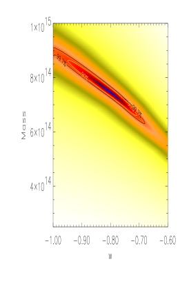
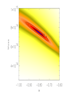
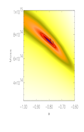
Figure 5: Confidence levels in the $w$-mass plane. The input model is a lens with an NFW profile with mass $M=7.5\times 10^{14}~{}h^{-1}M_{\odot}$ at $z=0.6$ in a cosmological model with $w=-0.8$. The contours shown by the dark curve correspond to a probability level of $99.7\%$. The three panels correspond to constraints from two arcs at $z=1$ and $z=2$ (left); from two arcs at $z=1$ and $z=2$ plus velocity dispersion at $10$ kpc from the centre (middle); from three arcs at $z=0.8$, $z=2$ and $z=3$ plus velocity dispersion at $10kpc$ from the centre (right). Note that these constraints apply only for the smooth analytical model we have used.

We notice that the sensitivity of the displacement of the critical curves to these lens properties changes as we vary the equation of state of dark energy. This reflects the different evolution of halos of a given mass in different cosmologies. As shown by BA02.1; BA03.1; DO03.2, the formation epoch of dark-matter halos with the same mass in these cosmological models is significantly different, leading to substantially different concentration parameters of the halo density profiles. Halos tend to form earlier and thus have typically larger concentrations in the SUGRA and in the DECDM models compared to the RP and the $\Lambda$CDM models. Thus, for these models, the growth rate of the critical curves is less sensitive to changes in redshift, mass and ellipticity.

3.4 Degeneracies in NFW models

Since the expansion of the critical curves as a function of the source redshift is different for halos with different concentrations, a degeneracy between mass and cosmology arises in NFW halos. That is, the same displacement of the critical curves for sources at two redshifts can occur with halos of different concentrations in more than one cosmological models. As shown in Sect. 3.1, the concentration is related to halo mass in NFW models of clusters.

For probing this degeneracy, we carry out the following test. We use an input model consisting of a lens of mass $M=7.5\times 10^{14}\,h^{-1}\,M_{\odot}$ at redshift $z_{\rm l}=0.6$ in a cosmological model with $w=-0.8$. We consider its critical curves for source redshifts $z_{\rm s}=1$ and $z_{\rm s}=2$, mimicking the constraints from two tangential arcs, and we fit their positions by varying the equation of state of dark energy and the lens mass. For simplicity, we consider only cosmologies with time-independent $w$. The fit is performed by minimising

$$\chi_{1}^{2}=\left(\frac{x_{1}(M,w)-\hat{x}_{1}}{\Delta_{1}}\right)^{2}+\left(\frac{x_{2}(M,w)-\hat{x}_{2}}{\Delta_{2}}\right)^{2}\;,$$ (22)

where $\hat{x}_{1}$ and $\hat{x}_{2}$ are the positions of the tangential critical curves of the input model for sources at $z_{\rm s}=1$ and $z_{\rm s}=2$, respectively, $\Delta_{1}$ and $\Delta_{2}$ are their respective errors, and $x_{1}(M,w)$ and $x_{2}(M,w)$ are the corresponding positions of the critical curves predicted by the fitting model with mass $M$ in a cosmological model with dark-energy equation of state $w$. We assume here to be in an idealized situation where the location of the critical curves is known at the $1\%$ level.

We show the confidence levels in the $w$-$M$ plane resulting from this fitting procedure in the upper left panel of Fig. 5. The innermost and the outermost contours correspond to probability levels of $68\%$ and $99.7\%$, respectively. As anticipated, a good fit to the position of the critical curves is obtained for a range of $M$ and $w$, with $99.7$ confidence limits ranging between $6\times 10^{14}\,h^{-1}\,M_{\odot}\la M\la 9\times 10^{14}\,h^{-1}\,M_{\odot}$ and $-1\la w\la-0.65$ (see also CH02.2).

For breaking this degeneracy, we must add constraints on the lens density profile. One possibility is to use the stellar velocity dispersion data for the brightest cluster galaxies in conjunction with the arc positions and redshifts (see MI95.1; SA03.1, and references therein). Including this additional constraint in our fitting procedure, we re-define our $\chi^{2}$ variable as

$$\chi^{2}_{2}=\chi^{2}_{1}+\left(\frac{\sigma_{r}(M,w)-\hat{\sigma}_{r}}{\Delta_{\sigma_{r}}}\right)^{2}\;,$$ (23)

where $\hat{\sigma}_{r}$ is the velocity dispersion of the input model at $10\,h^{-1}$kpc from the centre, $\Delta_{\sigma_{r}}$ is the uncertainty in its measurement, and $\sigma_{r}(M,w)$ the value predicted by the fitting model. For calculating the velocity dispersion from the density profile we use the spherical Jeans equation, assuming isotropic orbits,

$$\frac{\mathrm{d}\rho(r)\sigma_{r}(r)}{\mathrm{d}r}=-\frac{GM(r)\rho(r)}{r^{2}}\;,$$ (24)

where $G$ is the gravitational constant and $M(r)$ is the mass enclosed within a sphere of radius $r$. Again, we assume that the velocity dispersion at the chosen radius is known with an accuracy of $1\%$. This is a rather optimistic assumption, but our primary aim here is to discuss what kind of constraints are required for breaking the degeneracy. The new map of the confidence levels is shown in the upper right panel of Fig. 5. Although the contours shrink, some degeneracy remains, indicating that further constraints on the lens density profile are needed.

Finally, we use a lensed image from a third source at redshift $z_{\rm s}=3$ for locating another critical curve, in addition to two at $z_{\rm s}=0.8$ and $z_{\rm s}=2$ and to the velocity dispersion constraints. This allows us to distinguish among different cosmological models becomes easier as shown in the right panel of Fig. 5, but does require that we get lucky with the arc redshifts. It is also valid only for the smooth mass distribution represented by our analytical model; real clusters are likely to have a more lumpy structure.

Our simplified analysis with analytical NFW models for cluster halos was aimed at understanding the sensitivity of arc locations to variations in several physical parameters. Our results show that to get robust constraints on cosmology from a single cluster, a detailed modelling of the lensing mass distribution is required (see also CH02.2; DA03.1). This modelling would include the contribution from sub-structure in the cluster which we have not studied in our analytical models. Further, as shown by DA04.1, structures along the line of sight provide a source of error in modelling individual clusters that is very difficult to overcome.

4 Numerical models

4.1 Cluster sample

Since asymmetries and substructures play a crucial role in determining the strong lensing properties of galaxy clusters (ME03.1), analytic models can only be used for an approximate description of their lensing properties. More realistic mass distributions of clusters, as provided by numerical simulations, are needed for drawing quantitative conclusions. We now repeat the analysis previously applied to analytic models to a sample of numerical clusters.

The sample of clusters we use here consists of the 17 halos used by DO03.2 and ME04.1. We briefly summarise their main properties. The cluster models are pure dark-matter halos and were obtained using the most recent version of the cosmological code GADGET (SP01.1). The code was extended by DO03.2 to cosmological models with dynamical dark energy. Each cluster was obtained by resimulating at higher resolution a patch of a pre-existing large-scale cosmological simulation (TO97.2). The initial conditions were set up with the purpose of obtaining identically comparable clusters in all the cosmologies at redshift $z=0$. Of course, at higher redshifts, each of them appears at different evolutionary stages in different cosmologies, since the growth of the density perturbations depends on the equation of state of the dark energy. For example, clusters form earlier in the SUGRA and the DECDM compared to the RP and the $\Lambda$CDM models. The implications of the different time evolution of these clusters for different equations of state of dark energy on the abundance of strong lensing events is discussed in detail by ME04.1.

The clusters in the sample contain on average $N_{V}\approx 200,000$ dark matter particles within their virial radii. The corresponding virial masses range between $M_{V}=3.1\times 10^{14}$ to $1.7\times 10^{15}\,h^{-1}\,M_{\odot}$ at redshift zero.

4.2 Lensing simulations

Figure 6: Example showing how the critical curves of a numerical cluster at $z_{\rm l}=0.6$ simulated in different cosmological models change between $z_{\rm s}=1$ and $z_{\rm s}=2$

For each of them we take the snapshot at redshift $z_{\rm l}=0.6$ and perform lensing simulations. We first select from the simulation box a cube of comoving side length $3\,h^{-1}$Mpc. The three-dimensional mass distribution of the cluster is projected on a regular grid of $256\times 256$ cells along three orthogonal axes. The resulting two-dimensional density fields are smoothed using the Triangular Shaped Cloud method (HO88.1) for avoiding discontinuities between neighbouring cells. Thus, we analyse 51 projected lens mass distributions.

Through each of the surface density maps, we trace a bundle of $1024\times 1024$ light rays on a regular grid covering the central $1\,h^{-1}$Mpc² of the lens plane. This is large enough for enclosing the critical curves of all our numerical models. Deflection angles are computed using the method described in ME00.1. We first define a grid of $128\times 128$ “test” rays, for each of which the deflection angle is calculated by directly summing the contributions from all cells on the surface density map $\Sigma_{i,j}$,

$$\vec{\hat{\alpha}}_{h,k}=\frac{4G}{c^{2}}\sum_{i,j}\Sigma_{i,j}A\frac{\vec{x}_{h,k}-\vec{x}_{i,j}}{|\vec{x}_{h,k}-\vec{x}_{i,j}|^{2}}\;,$$ (25)

where $A$ is the area of one pixel on the surface density map and $\vec{x}_{h,k}$ and $\vec{x}_{i,j}$ are the positions on the lens plane of the “test” ray ($h,k$) and of the surface density element ($i,j$). Following WA98.2, we avoid the divergence when the distance between a light ray and the density grid-point is zero by shifting the “test” ray grid by half-cells in both directions with respect to the grid on which the surface density is given. We then determine the deflection angle of each of the $1024\times 1024$ light rays by bi-cubic interpolation between the four nearest test rays.

The reduced deflection angle is

$$\vec{\alpha}(\vec{x})=\frac{D_{\rm ls}}{D_{\rm s}}\vec{\hat{\alpha}}(\vec{x})\,.$$ (26)

Since we wish to estimate the growth of the tangential critical curves as a function of source redshift, we consider sources between $z_{\rm s}=1$ and $z_{\rm s}=2$.

Since the reduced deflection angle is the gradient of the lensing potential,

$$\vec{\nabla}\psi(\vec{x})=\vec{\alpha}(\vec{x})\,,$$ (27)

the convergence and the shear can be easily written as:

$$\kappa(\vec{x}) = \frac{1}{2}\left(\frac{\partial\alpha_{1}}{\partial x_{1}}+\frac{\partial\alpha_{2}}{\partial x_{2}}\right)$$ (28)

$$\gamma_{1}(\vec{x}) = \frac{1}{2}\left(\frac{\partial\alpha_{1}}{\partial x_{1}}-\frac{\partial\alpha_{2}}{\partial x_{2}}\right)$$ (29)

$$\gamma_{2}(\vec{x}) = -\frac{\partial\alpha_{1}}{\partial x_{2}}=-\frac{\partial\alpha_{2}}{\partial x_{1}}\ .$$ (30)

The tangential critical curves are then determined by searching for those points in the lens plane where Eq. (9) is satisfied.

4.3 Critical-curve sizes

The critical curves for one of the clusters in our sample in the different cosmological models are shown in Fig. 6. The sources are at redshift $z_{\rm s}=1$ in the upper panels and at $z_{\rm s}=2$ in the lower panels. Two important features are evident. First, for sources at redshift $z_{\rm s}$ the sizes of the critical curves differ substantially among the various cosmological models. For example, the cluster has almost no critical curves in the $\Lambda$CDM model, while they are already well developed in the SUGRA model. The RP and the DECDM models fall between these two cosmologies. This is a consequence of the earlier formation epoch of clusters in the RP, DECDM and in the SUGRA models than in the $\Lambda$CDM model (see e.g. BA02.1; BA03.1; DO04.1; ME04.1), due to which they have a larger concentration enabling them to be efficient lenses even at relatively high redshifts or for relatively close sources. Second, as expected from the analytical calculations, the relative enlargement of the critical curves is higher in the $\Lambda$CDM than in the other cosmological models.

Figure 7: Critical curve sizes normalized to $z_{s}=1$, as in Fig. 2, but for a numerical cluster sample comprising 17 halos placed at redshift $z_{\rm l}=0.6$. Only clusters producing critical curves for $z_{\rm s}=1$ are considered. Curves display the sample medians. The error bars show the first and the third quartile of the distribution, rescaled assuming that the information from $1000$ pairs of arcs could be combined.

We apply the same method used for the analytical models for estimating the size of critical curves of the numerical clusters. Fig. 7 shows the relative growth of the critical curves in the four cosmological models as measured in the numerical simulations. Each curve represents the median among the 51 halos which develop a critical curve for source redshift $z_{\rm s}=1$. The number of useful clusters for this analysis ranges between $\sim 20$ in the $\Lambda$CDM to $\sim 30$ in the SUGRA model. The results confirm the qualitative expectations from analytic models: namely, the trend for different cosmologies. The absolute values of the relative growth are also consistent with the predictions for a moderate ellipticity ($e\la 0.3$) lensing potential (compare Figures 2 and 7).

These results show that the statistical application of this method is potentially powerful. Upcoming surveys from space, like those which will be conducted by SNAP (AL04.1), could provide detailed observations of order thousand galaxy clusters, allowing the information from many lenses to be combined. The error bars in Fig. 7 show the first and the third quartiles of the curve distribution we obtain from our numerical cluster sample. They were rescaled to the expected error when the information from $\sim 1000$ pairs of arcs is combined. The figure shows that when constraints on the position of the critical curves from sources at significantly different redshifts and in a sufficiently large sample of clusters are used, it becomes possible to discriminate among different cosmological models. We have used a simple choice of source redshifts; by extending the analysis to a wider redshift range, especially to redshifts beyond 2 for the distant arcs, the constraints became stronger. The analysis needs to be extended in other ways as well, by combining the information from different lens redshifts and finding the best way to weight a given cluster.

In our test, we have used a simple estimate of the size of the critical curves, which we can assume is related to the cluster-centric distance of an observed arc, without any mass modelling of the cluster. We obtain substantially different amounts of growth of the critical curves depending on the level of substructure in the central region of the clusters. If the cluster is close to critical for sources at redshift $\sim 1$ at the location of a substructure, we measure a rapid growth of the critical curve once the sources are shifted to higher redshift. This occurs because the critical surface density becomes smaller and the cluster critical curves wiggle around the emerging critial mass lumps. This is shown for example in Fig. 6, where the shape of the critical curves changes dramatically between $z_{\rm s}=1$ and $z_{\rm s}=2$ for some of the cosmological models (see e.g. the DECDM model). If mass modelling for some of the clusters were to be included, the scatter in Fig. 7 could be reduced. Finally we note that to some extent carrying out such an analysis from observations would require simulations that correctly reproduce the properties of real clusters. While we have used only the relative locations of arcs at different redshifts, it is worth examining what aspects of cluster structure these are sensitive to.

4.4 Imaging surveys for cluster lensing

Strong lensing studies with galaxy clusters require high quality imaging data. While we will not examine the survey requirements in any detail, we have used our numerical clusters to produce lensed images of the Hubble Ultra Deep Field (HUDF). We can use these to study of the effects of sky brightness, photon noise and resolution on cluster arcs.

Figure 8 shows the kind of imaging expected from space imaging and current state of the art ground based imaging. Clearly, the demands on resolution are very high to reliably measure the properties of lensed arcs. With $0.5$ arcsecond imaging the quality of the images is compromised, as shown in the right panel, but the large arcs are still identified. Adaptive optics may enable better resolution images to be obtained than shown in this figure; short of that, it may still be possible to use giant arcs and on average get the arc separations accurately enough. Ideally, a space based survey that images a large number of multiple-arc clusters with resolution comparable to the HST would provide an adequate sample. For such a survey, the question of how deep it is worth going to find high-redshift arcs merits worth further study.

In addition to multi-color imaging, which would enable photometric redshift estimates, cluster cosmography would require spectroscopic redshifts for the lensed arcs. An important exercise for future work is to estimate the number of arcs expected from a realistic sample of clusters for given survey parameters. DA03.1 have used three existing cluster lensing datasets (GL03.1; LU99.1; ZA03.1) and estimated that of order 1000 arcs are expected on the sky even from a survey of modest depth. Given the landscape of proposed telescopes and surveys, it is not prohibitive to think high resolution imaging of order a thousand cluster containing fields, as well as follow-up spectroscopy on the several thousand arcs that might be found.

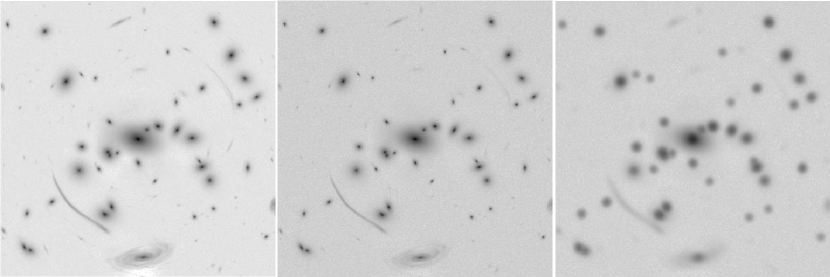
Figure 8: Simulated observations from a VLT-like telescope of the same field observed by HST in the ultra-deep field with $10^{6}$ sec exposure. The simulations include a sky brightness $I=19.9$ mag/arcsec², Poisson photon noise and a seeing of $0.5$ arcsec. The lensing cluster of galaxies is at $z=0.25$. The cluster members have been added by placing a cD galaxy at the cluster center and by distributing the other galaxies following the underlying dark matter mass distribution. The galaxy luminosity reflects that of realistic cluster members (spectral energy distribution, morphological type as a function of the the cluster-centric distance reproduce observational constraints). The integration time is 3000 sec. In the lensing simulation, all the sources were assumed to be at $z=2$. The field size is $~{}1$ arcminute along the x-axis. The middle panel includes sky brightness and Poisson photon noise; the right panel includes seeing.

5 Summary

This paper presents a study of cosmography with galaxy clusters that produce lensed arcs of background galaxies. Clusters with multiple arcs from different redshifts provide constraints on angular diameter distances at different redshifts. These in turn constrain the equation of state of the dark energy. We have studied this effect with analytical models to understand some of the qualitative trends, and with numerical simulations to see what can be expected from surveys of real clusters.

We have used analytical models of clusters based on the NFW profile to study how the positions of arcs depend on the mass distribution and the cosmological model. We find that the ellipticity and concentration of the cluster halo can shift the critical curves. Substructure would have the same effect. This means that for individual clusters, it is important to have independent information on the mass distribution, especially inside the critical curve, to extract cosmographic information from arc positions and redshifts. Our analysis overlaps with other recent studies of cluster arcs, e.g. CH02.2; OG03.1; ME03.1; DA03.1; WA03.1. We explore examples of how information from inner velocity dispersions and multiple arcs could be combined for a single cluster. However a more sophisticated study is warranted.

Given the limitations of analytical models (they cannot for example include the effect of substructure in the halos), we conclude that numerical modelling is essential to extract information from observed clusters. We use a sample of simulated clusters in four dark energy models in an exploratory study of whether future surveys can provide cosmographic information. We examine the scatter in the relative positions of arcs due to differences in the mass distributions of individual clusters. We focus on the critical curves and use these to estimate arc positions. While this is a simplified study, we believe it gives us a reasonable estimate of the minimum requirements of a cluster sample to overcome the cluster-to-cluster scatter and obtain cosmographic constraints.

In the numerical study we have not attempted to model the mass distribution of individual clusters. We have only used information on the relative sizes of critical curves at different redshifts. In practice, some constraints on the mass distributions will be obtained from strong and weak lensing, as well as X-Ray, SZ and velocity dispersion measurement. Further study is needed on how well this information can be used to improve cosmographic constraints. Further, we have used information only from arcs up to redshift 2; one would do better if imaging and spectroscopy on arcs at higher redshifts were available.

We have attempted to include the main sources of complexity that arise from the mass distribution of clusters. We have neglected several factors in the observation of clusters and their interpretation that merit further study. Structures along the line of sight at redshifts different from the cluster are an important source of scatter. DA04.1 have studied the impact of these structures; they find that they limit the use of individual clusters and could contribute to the error in dark energy parameters from an ensemble of clusters. Further we used just the positions of the largest arcs, and have largely ignored other strong lensing information as well as the measurement error in using arc positions. These factors are all important and require more detailed studies.

We have estimated the scatter in cosmographic constraints from different clusters. We have not addressed the question of how an actual survey would best average results from different clusters. Clearly some clusters will have multiple arcs (over 100 in the case of Abell 1689) and therefore contain more information. Others may have a regular, spherically symmetric structure which would make it easier to extract cosmographic information from arc positions.

While completing this study, we have learnt of a preprint by DA04.1 that examines sources of noise in arc-cosmography.