Constraints on the role of synchrotron X-rays from jets of accreting black holes

Abstract

We present an extension of the scale invariance formalism by Heinz & Sunyaev (2003) which includes the effects of radiative cooling on the X-ray synchrotron emission from core dominated jets and outflows. We derive the scaling relations between the radio luminosity $L_{\rm r}$, the synchrotron X-ray luminosity $L_{\rm x}$, the mass $M$, and the accretion rate $\dot{m}$ of an accreting black hole. We argue that the inclusion of synchrotron losses into the scaling relations is required by the data used in Merloni et al. (2003) to define the “fundamental plane” correlation between $L_{\rm r}$, $L_{\rm x}$, and $M$ in AGNs amd Galactic X-ray binaries. We then fit the new scaling relations to the “fundamental plane” correlation. This allows us to derive statistical constraints on the contribution from jet synchrotron emission to the X-rays from black holes, or, alternatively, on the particle acceleration scheme at work in these jets. We find that, in order for jet synchrotron X-rays to be consistent with the observed $L_{\rm r}-L_{\rm x}-M$ correlation, the global particle spectrum must be both steep: $f(\gamma)\propto\gamma^{-(3.4^{+0.6}_{-0.5})}$ and unbroken down to energies well below the radio synchrotron regime. Such a steep particle distribution would imply steeper X-ray spectra than observed in most sources contributing to the correlation with avalailable X-ray spectral index measurements. We suggest that, unless some assumptions of the scale invariance hypothesis are broken, another emission mechanism (likely either disk radiation and/or inverse Compton scattering in the jet) contributes significantly to the X-rays of a sizeable fraction of the sources.

1 Introduction

For many years, the standard paradigm for the X-ray emission in accreting black hole systems has been that the X-rays are produced in the central accretion flow (e.g., Shakura & Sunyaev, 1973; Shapiro et al., 1976; Narayan & Yi, 1994), while radio emission was traditionally attributed to a radio jet. Only in the most powerful, beamed jet sources was X-ray synchrotron and inverse Compton emission from the jet invoked to explain the featureless powerlaw spectra of Blazars and BL-Lacs (e.g. Fossati et al., 1998).

In recent years, however, this paradigm has been called into question. Beginning with a re–evaluation of the emission processes in Galactic X-ray binaries (XRBs), an alternative view has been proposed to interpret a large part of the spectrum (including X-rays) of black holes at moderate to low accretion rates entirely as due to the emission from the jet (Markoff et al., 2001, 2003; Falcke et al., 2004).

It has been difficult to find unique signatures that would allow us to distinguish between these two alternatives. Broad band spectral modeling is the most promising approach, but so far it has not been shown conclusively that either of the two approaches fails. The strong correlation between the radio and the X-ray emission in X-ray binaries that has been found recently (Corbel et al., 2003; Gallo et al., 2003) can be interpreted in terms of both pictures. Similarly, the correlation between radio luminosity $L_{\rm r}$, X-ray luminosity $L_{\rm x}$, and black hole mass $M$ is consistent with both pictures (Merloni et al., 2003; Falcke et al., 2004).

In order to investigate the relation between $L_{\rm xr}$, $L_{\rm x}$, and $M$, Heinz & Sunyaev (2003) derived robust and very general scaling relations between these observables which are independent of the underlying jet model (e.g. Blandford & Ostriker, 1978; Falcke & Biermann, 1995), provided that jet physics is scale invariant under changes in black hole mass $M$ and accretion rate $\dot{m}=\dot{M}/\dot{M}_{\rm Edd}$ (where $\dot{M}_{\rm Edd}$ is the Eddington accretion rate). The striking agreement with the subsequently found “fundamental plane” relation of accreting black holes (Merloni et al., 2003; Falcke et al., 2004) seems to confirm the scale invariance hypothesis.

The original treatment of Heinz & Sunyaev (2003) did, however, leave out some critical physical ingredients required to describe the X-ray synchrotron emission from jets, namely, radiative cooling of the particle distribution, which alters the spectral shape at higher energies. In this paper, we will present an extension of the formalism developed in Heinz & Sunyaev (2003) that allows us to include radiative cooling (§2 and §A.1). We then proceed to investigate the data of the “fundamental plane” relation for signs of radiative cooling and discuss limits we can put on the contribution of X-ray synchrotron radiation from jets to the spectra of AGNs and XRBs by fitting the derived scaling relations to the fundamental plane correlation (§3). Section 4 summarizes the conclusions we draw from this analysis.

2 Scale invariance in jets with radiative losses

In Heinz & Sunyaev (2003) we derived the scaling relations between synchrotron radio luminosity $L_{\rm r}$, black hole mass $M$, and accretion rate $\dot{M}$. Because radiative losses introduce another scale into the problem, we chose to ignore the effect of synchrotron cooling on the particle distribution, given the scope of the paper. As we will show below, it is possible to incorporate these effects without loss of generality, because the scale introduced by cooling depends itself only on the mass and accretion rate of the black hole and does not enter into the dynamical properties of the jet plasma at all. This is because cooling affects primarily the highest energy particles, while most of the jet kinetic energy and thrust are carried by the low energy particles (in other words, jets are believed to be radiatively inefficient).

2.1 The scale invariance hypothesis for cooled jets

In order to include the effects of radiative cooling into the scale invariance formalism (Heinz & Sunyaev, 2003), we shall briefly review the aspects of the scale invariance ansatz relevant to this article. For a detailed discussion, we refer the interested reader to the original article.

The scale invariance ansatz assumes that there is only one relevant scale in the problem of jet dynamics (at least in the cores of jets which we are focusing on here): the gravitational radius $r_{\rm g}=GM/c^{2}$. It also assumes that the structure of all core jets¹ from black holes is the same when set in relation to $r_{\rm g}$. Mathematically, the scale invariance assumption can be formulated as the requirement that any dynamical quantity $f$ relevant to calculating the synchrotron emission from jets (such as the normalization of the powerlaw distribution of electrons, the magnetic field, or the particle pressure) can be decomposed into two functions $\phi_{f}(M,\dot{m})$ and $\psi_{f}(\chi)$, such that

$$f(M,\dot{m},r)=\phi_{f}(M,\dot{m})\psi_{f}(\chi)$$ (1)

where the definition $\chi=r/r_{\rm g}$ implies that $\psi_{f}$ depends only on scale–free coordinates $(x,y,z)/r_{\rm g}$.

The functions $\phi_{f}$ define the normalization of $f$ at the base of the jet (as provided by the accretion disk), while the structure functions $\psi_{f}$ describe the variation of $f$ along the jet, relative to its value at the base of the jet. Any non-trivial dependence of $f$ on the black hole spin $a$ is assumed to be implicit in the functions $\psi_{f}$ and will not be discussed further. For consistency, we will also assume that the jet velocity $\beta\Gamma$ is independent of black hole mass and accretion rate, such that $\beta\Gamma=\psi_{\beta\Gamma}(\chi)$. It is still not known what the true jet plasma velocities are, especially close to the base of the jet, but future constraints will hopefully shed some light on this subject. If this assumption is not satisfied, the formalism can easily be altered to include such an $M$ or $\dot{m}$ dependence as long as the four-velocity $\beta\Gamma$ can be written in the form of eq. (1).

Given these assumptions, we can proceed to include radiative cooling into the treatment. We will assume that a fraction of the jet particles are accelerated at some arbitrary time $t_{0}$ (measured in the jet frame) into a powerlaw such that

$$f(\gamma,t_{0})=\phi_{C}\gamma^{-p}$$ (2)

and then evolve through adiabatic and radiative cooling as they move downstream from the acceleration region.

While it is not necessary to assume that this acceleration takes place in one particular location (it can be spatially extended, in which case the integral in eq. (A.2) can be performed in a piece-wise fashion for every acceleration zone), it will be necessary to make the assumption that the spatial distribution of the acceleration (i.e., the various positions of the acceleration regions measured in units of gravitational radii $r_{g}$) and the shape of the powerlaw are invariant under changes of $M$ and $\dot{m}$ (in line with the assumptions necessary to derive the original scale invariance properties in Heinz & Sunyaev 2003). This implies that the injection time in the jet frame $t_{0}$ is proportional to $t_{0}\propto r_{\rm g}\propto M$. This is reasonable if the particle acceleration is associated with a hydrodynamic process, such as a recollimation shock, since the underlying hydrodynamics is also assumed to be scale invariant.

Furthermore, we will assume that the particle pressure is dominated by the low energy end of the particle distribution, which implies that the slope of the particle distribution produced by the acceleration process is steeper than $p\mathrel{\hbox{\hbox to0.0pt{\hbox{\lower 4.0pt\hbox{$\sim$}}\hss}\hbox{$>$}}}2$. Classical Fermi I shock acceleration in strong, non-relativistic shocks produces spectra with index $p\mathrel{\hbox{\hbox to0.0pt{\hbox{\lower 4.0pt\hbox{$\sim$}}\hss}\hbox{$>$}}}2$ (Blandford & Ostriker, 1978; Bell, 1978; Drury et al., 1982), while the spectral index produced in strong relativistic shocks is somewhat steeper, $p\sim 2.3$ (Gallant et al., 1999; Achterberg et al., 2001).

These indices agree nicely with the observed optically thin radio synchrotron spectra of extended jets with spectral indices of order $0.5\mathrel{\hbox{\hbox to0.0pt{\hbox{\lower 4.0pt\hbox{$\sim$}}\hss}\hbox{$<$}}}\alpha_{\rm r}\mathrel{\hbox{\hbox to0.0pt{\hbox{\lower 4.0pt\hbox{$\sim$}}\hss}\hbox{$<$}}}0.7$ (where the radio spectral index is defined as $\alpha_{\rm r}\equiv-\partial{(\log{F_{\rm r}})}/\partial{(\log{\nu})}$). For this reason, we will assume in the following that the fiducial spectral index of the uncooled electron distribution falls into the range $2\leq p\leq 2.3$. The fiducial uncooled synchrotron spectral index falls into the range $0.5\leq\alpha\leq 0.65$. More recent efforts studying particle acceleration in jets are focusing on continuous particle acceleration mechanisms like reconnection (e.g. Larrabee et al., 2003), which might be necessary to explain the lack of synchrotron cooling signatures in some extended AGN jets like 3C273 (Jester et al., 2001).

2.2 Scaling relations

With the basic set of assumptions in place, we proceed to derive the scaling relations for the X-ray synchrotron emission from jet cores including the effects of radiative cooling on the particle distribution. The complete mathematical derivation used in the remainder of this paper is presented in the appendix. For the casual reader, we will present a sketch of the derivation in the following paragraphs.

Synchrotron cooling of a population of electrons in the presence of a source of fresh powerlaw particles (which is the appropriate model for a continuous jet) will produce a cooling break in the global spectrum, as sketched in Fig. 1. Given the field strength $B$, the characteristic “cooling energy” of this break in the electron spectrum is (e.g. Rybicki & Lightman, 1979, also, see eqs. (21a) and (22) for a derivation of this expression) $\gamma_{\rm b}\sim\left[{A_{0}B^{2}t_{\rm jet}}\right]^{-1}$, where $t_{\rm jet}\sim r_{\rm jet}/v_{\rm jet}\propto M$ is the characteristic travel time of the electrons. Using eq. (1), this expression becomes $\gamma_{\rm b}\propto{\phi_{\rm B}(M,\dot{m})}^{-2}M^{-1}$. The characteristic synchrotron frequency corresponding to this electron energy is

$$\nu_{\rm b}\propto B\gamma_{\rm b}^{2}\propto\left[\phi_{\rm B}(M,\dot{m})\right]^{-3}M^{-2}$$ (3)

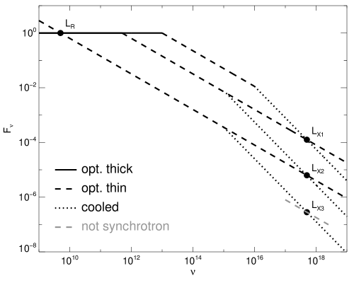
Figure 1: Sketch of viable synchrotron spectra in different regimes for three different measured radio-to-X-ray ratios. Optically thick parts are shown as solid lines, optically thin, uncooled parts are shown as dashed lines, optically thin, radiatively cooled parts are shown as dotted lines. The grey dashed line through L_X3 shows an X-ray spectrum that is flatter than the global spectrum, which would require a concave spectrum and would be inconsistent with simple synchrotron X-rays.

We will assume that the spectrum has a break at $\nu_{\rm b}$ with powerlaw index $\alpha_{\rm x}$ above $\nu_{\rm b}$ and with the standard powerlaw index $\alpha=(p-1)/2$ below $\nu_{\rm b}$ (see sketch in Fig. 1). Given the expression for $\nu_{\rm b}$ from eq. (3), the flux at a fixed frequency $\nu_{\rm x}$ above the cooling break $\nu_{\rm b}$ is a simple function of the flux $F_{\nu_{0}}$ at a fixed frequency $\nu_{0}$ below the cooling break, the black hole mass $M$, and the accretion rate $\dot{m}$:

$$F(\nu_{\rm x})=F_{\nu_{0}}\left(\frac{\nu_{\rm 0}}{\nu_{\rm b}}\right)^{(p-1)/2}\left(\frac{\nu_{\rm b}}{\nu_{\rm x}}\right)^{-\alpha_{\rm x}}$$ (4)

The uncooled, optically thin jet flux $F(\nu_{0})$ depends on $M$ and $\dot{m}$ as follows (Heinz & Sunyaev, 2003):

$$F(\nu_{0})\propto M^{3}\phi_{B}^{\frac{p+1}{2}}(M,\dot{m})\phi_{C}(M,\dot{m})$$ (5)

With the expression for $F(\nu_{\rm x})$ as a function of $F(\nu_{0})$, $M$, and $\dot{m}$ from above, we have

$$F(\nu_{\rm x})\propto M^{2+p-\alpha_{\rm x}}\phi_{B}^{2p-1-3\alpha_{\rm x}}\phi_{C}$$ (6)

Writing this expression in differential form, we arrive at the scaling relation derived in full generality in the appendix in eq. (35) and eq. (36)

We expect the functions $\phi_{B}(M,\dot{m})$ and $\phi_{C}(M,\dot{m})$ to be of powerlaw type, given typical accretion disk scenarios; Heinz & Sunyaev (2003) and Merloni et al. (2003) discuss the possible functional forms of $\phi_{B}$ and $\phi_{C}$. In this case, the logarithmic derivatives $\xi_{\rm xM}$ in eq. (35) and $\xi_{\rm x\dot{m}}$ in eq. (36) are constant and the scaling relation between $F_{\rm x}$ and $M$ and between $F_{\rm x}$ and $\dot{m}$ assumes powerlaw form:

$$F_{\rm x} \propto M^{\xi_{xM}}\dot{m}^{\xi_{x\dot{m}}}$$ (7)

$$\xi_{\rm xM} = 2-2\alpha_{\rm x}+p+\frac{\partial\log{(\phi_{C}})}{\partial\log{M}}$$ (8)

$$+(2p-1-3\alpha_{\rm x})\frac{\partial\log{(\phi_{B})}}{\partial\log{M}}$$

$$\xi_{\rm x\dot{m}} = \frac{\partial\log{(\phi_{C}})}{\partial\log{\dot{m}}}+(2p-1-3\alpha_{\rm x})\frac{\partial\log{(\phi_{B})}}{\partial\log{\dot{m}}}$$ (9)

Expressing the scaling relation this way is useful because $p$ and $\alpha_{\rm x}$ are actually observables. In other words, we can substitute observable quantities (in this case the X-ray and the particle spectral indices $\alpha_{\rm x}$ and $p$ respectively) for the unknown details of particle acceleration and cooling. It is important to keep in mind that $p$ is the electron spectral index produced by the acceleration process, i.e. below the cooling break and thus without any modification due to cooling. $p$ is therefore not observable via the X-ray spectral index. Rather, optically thin, uncooled radio, sub-millimeter, or IR emission should be used to infer $p$, since this radiation should not be affected by synchrotron losses.

In the following we will use the same canonical functional forms for $\phi_{B}$ and $\phi_{C}$ used in (Heinz & Sunyaev, 2003). Namely, we assume that the underlying accretion flow is mechanically cooled, in which case the accretion flow itself is scale invariant. Then

$$\phi_{C}={\phi_{B}}^{2}=\dot{m}M^{-1}$$ (10)

This prescription is also valid for coronae above gas pressure-dominated, radiatively efficient (Shakura & Sunyaev, 1973) accretion disks (the standard scenario for the origin of powerlaw X-ray emission and the launching point for jets from geometrically thin accretion disks, e.g. Merloni & Fabian, 2002). We then have

$$\xi_{{\rm x}M} = \frac{3-\alpha_{\rm x}}{2}$$ (11)

$$\xi_{{\rm x}\dot{m}} = p+\frac{1-3\alpha_{\rm x}}{2}$$ (12)

These are the expressions we will use in the remainder of this paper to fit the “fundamental plane” correlation. In the uncooled limit of $\alpha_{\rm x}=(p-1)/2$, they reduce to the expressions derived for the optically thin case from eq. (5). In the canonical case of $p=2$, we have $F_{\rm x}\propto M^{(3-\alpha_{\rm x})/2}{\dot{m}}^{(5-3\alpha_{\rm x})/2}$.

Since the “fundamental plane” correlation is measured between the radio and X-ray luminosities and the black hole mass, we should convert the scaling relations to those coordinates. From Heinz & Sunyaev (2003), the radio flux follows the scaling relation

$$F_{\rm r}\propto M^{\frac{2p+13-(2+p)\alpha_{\rm r}}{8+2p}}{\dot{m}}^{\frac{2p+13+(p+6)\alpha_{\rm r}}{2\left(p+4\right)}}$$ (13)

Combining this expression with eqs. (11) and (12), we finally arrive at the desired relation between $F_{\rm r}$, $M$, and the synchrotron X-ray emission $F_{\rm x}$:

$$F_{\rm r} \propto M^{\xi_{\rm RM}}{F_{\rm x}}^{\xi_{\rm RX}}$$ (14)

$$\xi_{\rm RM} = \frac{\left(2p+13-\left(2+p\right)\alpha_{\rm r}\right)\left(p-1-\alpha_{\rm x}\right)-\left(2\alpha_{\rm r}\right)}{\left(p+4\right)\left(2p+1-3\alpha_{\rm x}\right)}$$ (15)

$$\xi_{\rm RX} = \frac{2p+13+\left(p+6\right)\alpha_{\rm r}}{\left(p+4\right)\left(2p+1-3\alpha_{\rm x}\right)}$$ (16)

This can now be compared directly to the measured correlation coefficients $\xi_{\rm RM,FP}=0.78$ and $\xi_{\rm RX,FP}=0.6$.

3 Constraints on the X-ray emission mechanism

The “fundamental plane” correlation has the form

$$\log{L_{\rm r}}=0.78\log{M}+0.6\log{L_{\rm x}}+7.33$$ (17)

Merloni et al. (2003) interpreted this correlation in terms of the scale invariance model. From the observed correlation, it is unclear whether the source of the X-rays is, in fact, synchrotron emission from the jet, or whether it is emission from an inefficiently accreting disk; both can produce similar correlation coefficients in the context of the scale invariance model. The scaling relations for inefficient disk X-rays do produce a better fit to the fundamental plane, but Merloni et al. (2003) noted that the effects of synchrotron losses on the synchrotron X-ray emission from the jet had not been included in their treatment and might improve the fit to the fundamental plane data. Given the analysis presented in the previous section, we can now proceed to include these effects and test whether they improve the fit or not.

3.1 Spectral evidence for synchrotron cooling

Before applying the scaling relations derived in eqs. (15) and (16) to the “fundamental plane” sample, we shall present a brief argument that the inclusion of cooling into the scale invariance relations presented above is not just useful, but actually necessary to properly interpret the fundamental plane data in the context of synchrotron jet X-rays.

First, we will check the global radio-X-ray spectra of individual sources against the hypothesis that the X-rays originate in the jet as optically thin, uncooled synchrotron emission. In this case, the X-ray spectrum should continue from the X-rays to lower frequencies at the standard synchrotron spectral index $\alpha_{\rm x}=(p-1)/2$, until it reaches the turnover frequency where the jet becomes optically thick to synchrotron self absorption (see Fig. 1). At this point, the spectrum becomes flat. This implies that the spectrum is convex at every point between the radio and X-ray bands.

Therefore, if the global spectral index $\alpha_{\rm rx}$ is steeper than the fiducial uncooled X-ray spectral index $\alpha_{\rm X}=(p-1)/2$, radiative cooling must have steepened the jet synchrotron spectrum at X-ray energies (this corresponds to point $\rm L_{\rm X3}$ in Fig. 1). Only a cooling break/cutoff can reduce the X-ray flux to the observed level (even if the radio spectrum is optically thick). This constraint corresponds to the horizontal dashed grey line in Fig. 2, and a number of sources lie above this line, showing that radiative cooling must be included in the treatment of these sources. Note that relativistic beaming and uncorrelated radio/X-ray variability do not change this conclusion.

On the other hand, if the global spectral index $\alpha_{\rm rx,FP}$ is flatter than the fiducial uncooled synchrotron spectrum (point $\rm L_{X1}$ in Fig. 1, all points below the dashed grey line in Fig. 2), we cannot say anything about the action of radiative cooling. All we can conclude in this case is that either the radio synchrotron emission must be self-absorbed (thus flattening the global synchrotron spectrum), or the X-rays must be from the disk (thus increasing the X-ray flux relative to the radio).

For a sub-set of the sources in the “fundamental plane” sample, the X-ray spectral indices $\alpha_{\rm x}$ have actually been measured, though for some sources with very large error bars. All of these sources are AGNs, as the RXTE-ASM data used in compiling the “fundamental plane” sample are not sufficient to determine the spectral slope between 2 and 10 keV. However, we note that for XRBs in the low-hard state, where the radio-X-ray correlation is observed to hold, the X-ray powerlaw spectra are typically hard - with $0.5\mathrel{\hbox{\hbox to0.0pt{\hbox{\lower 4.0pt\hbox{$\sim$}}\hss}\hbox{$<$}}}\alpha_{\rm x}\mathrel{\hbox{\hbox to0.0pt{\hbox{\lower 4.0pt\hbox{$\sim$}}\hss}\hbox{$<$}}}1.0$. Most of what will be discussed regarding the AGN with measured $\alpha_{\rm x}$ will also hold for these sources.

We have plotted the global and X-ray spectral indices of all AGNs in the sample where $\alpha_{\rm x}$ has been measured in Fig. 2. This figure shows several interesting things:

• Some sources have global spectra steeper than $\alpha_{\rm rx}>0.65$ (above the dotted grey line), which implies that they are affected by cooling or have unusually steep particle spectra. Because XRBs are generally less radio loud than AGNs, all XRBs fall well below this line (they are not shown on this plot for lack of $\alpha_{\rm x}$ measurements), thus, this observational constraint on the importance of cooling is not available for XRBs.

• Most of the sources in the plot have X-ray spectra steeper than the fiducial uncooled synchrotron spectrum of $\alpha_{\rm X}>0.65$ (right of dashed grey line). This indicates that, if the X-rays are due to synchrotron emission, (1) radiative cooling should have altered their spectrum or (2) the particle injection spectrum must be steeper than typical Fermi I shock acceleration.

• About 25% of the sources in the plot actually fall into the area left of the solid black line where the X-ray spectral index is flatter than the global spectral index (corresponding to the dashed grey line through point $\rm L_{X3}$ in Fig. 1), i.e., $\alpha_{\rm x}<\alpha_{\rm rx}$. These sources have concave global spectra and the X-rays from these sources cannot be due to X-ray synchrotron emission from the jet, unless a particle acceleration scheme is at work that produces concave electron spectra. Again, all XRBs lie well below this line, so this observational constraint on the nature of the emission mechanism is not available for XRBs. We note that the error bars on $\alpha_{\rm x}$ for all of the sources left of the line are large. Thus, it is prudent not to draw any firm conclusions from this seeming discrepancy at this point and await better observational determinations of $\alpha_{\rm x}$ for these sources.

In summary, we find that radiative cooling must be at work in most of the AGNs contributing to the “fundamental plane” sample, unless the particle spectra are intrinsically somewhat steeper than those produced in Fermi I acceleration and typically observed in optically thin radio synchrotron spectra of relativistic jets. This underlines the need for radiative cooling to be included in properly modeling the “fundamental plane” correlation.

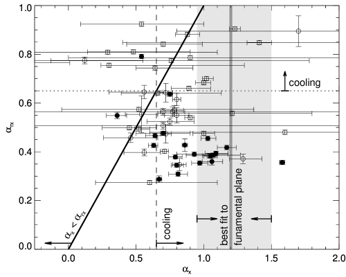
Figure 2: Plot of the measured radio-X-ray spectral index $\alpha_{\rm rx}$ against the measured X-ray spectral index $\alpha_{\rm x}$ for the AGNs in the “fundamental plane” sample where this information is available. left of black line: X-ray spectrum flatter than radio-to-X-ray spectrum, $\alpha_{\rm x}<\alpha_{\rm rx}$, difficult to reconcile with global synchrotron spectrum; light grey area: X-ray spectral indices from best fit to “fundamental plane” correlation (see Fig. 3); dashed and dotted grey lines: cooling or steep injection spectrum necessary to the right of and above these lines; filled dots: sources with X-ray luminosity $L_{\rm x}>10^{-3}\,L_{\rm Edd}$, empty dots: sources with $L_{\rm x}<10^{-3}\,L_{\rm Edd}$.

3.2 Fitting the scaling relations to the “fundamental plane” data set

We will now compare the new scaling relations to the fundamental plane correlation. We will assume in the following that the radio emission is unaffected by radiative cooling. Therefore, if the X-rays originate in the disk, the scaling relations from the scale invariance model (Heinz & Sunyaev, 2003) are unaltered and we will not discuss them any further, apart from reminding the reader that they provide the best fit to the observed correlation, provided that the disk emission is radiatively inefficient, (with $L_{\rm x}\propto{\dot{m}}^{2}$ Merloni et al., 2003).

If the X-rays originate in the jet, however, we must include radiative cooling, based on the arguments presented in §3.1. The presence of a cooling break in the spectrum was already discussed in §2. We define the magnitude of the break as $\Delta\alpha_{\rm x}\equiv\alpha_{\rm x}-(p-1)/2$. We will assume in the following that this break lies below the X-ray band for all sources of interest. If this were not the case, the break would move through the X-ray band and produce an observable change in the correlation coefficients. Given the scatter in the “fundamental plane” relation, we cannot rule out such a change with any certainty. We note that the presence of such a change would be an indication of jet X-rays. The dependence of the break frequency $\nu_{\rm b}$ on $M$, $\dot{m}$ (or alternatively, $F_{\rm x}$), and the radio luminosity $L_{\rm r}$ can be easily calculated from eqs. (22) and (29) and compared to future data.

We will now use eqs. (15) and (16) to test whether radiative cooling will improve the fit of synchrotron X-rays to the “fundamental plane” correlation. In the simplest possible case of continuous injection of fresh powerlaw particles with index $p$ (e.g., by a stationary shock) without any adiabatic losses, the spectral break produced by cooling is $\Delta\alpha_{\rm x}=1/2$. Thus, for a canonical synchrotron spectrum of index $p=2$, $\alpha=1/2$, and $\Delta\alpha_{\rm x}=1/2$, the steepened spectrum above the break has a powerlaw index of $\alpha_{\rm x}=1$. Inserting this value into eqs. (15) and (16) gives $F_{\rm x}\propto M\dot{m}$ and thus $\xi_{\rm RM}=0$ and $\xi_{\rm RX}=1.42$.

This implies that cooled synchrotron emission from the jet follows the exact same scaling relation as efficient disk X-rays. As shown in Merloni et al. (2003), radiatively efficient disk X-rays are inconsistent with the observed correlation coefficients of the “fundamental plane”. This is clear from comparing $\xi_{\rm RM}=0$ and $\xi_{\rm RX}=1.42$ with the measured correlation coefficients of $0.78$ and $0.6$ respectively. Thus, jet X-rays, in the most straightforward scenario of synchrotron emission (which includes cooling and the canonical range of particle spectral indices), are not compatible with the observed correlation.

We can ask the broader question under what conditions the scaling relations predicted by synchrotron X-rays are actually consistent with the observed correlation coefficients. We will do this by fitting the “fundamental plane” data set with the correlation coefficients $\xi_{\rm RM}$ and $\xi_{\rm RX}$ from eqs. (15) and (16). We will ignore upper limits in the data and use the same merit chi-square estimator employed in Merloni et al. (2003); Gebhardt et al. (2000). We also use the same error estimate, i.e., we assume isotropic errors in all variables and normalize them such that the reduced chisquare of the best fit is one. This is equivalent to equating the scatter in the fundamental plane to the uncertainty and is a conservative approach for calculating errors.

Figure 3 shows a chi-square map for the two interesting parameters $\Delta\alpha_{x}$ and $p$ (marginalized over the unknown relative normalization between radio and X-ray flux). As expected, the figure shows that a standard cooled synchrotron spectrum with $p=2$ and a cooling break of $\Delta\alpha_{\rm c}=0.5$ is inconsistent with the correlation coefficients derived from the “fundamental plane” relation by more than 3 sigma. The best fit actually requires a steep, unbroken powerlaw with $p=3.4^{+0.6}_{-0.5}$, $\Delta\alpha_{\rm c}=0^{+0.13}_{-0}$ and $\alpha_{\rm x}=1.2^{+0.3}_{-0.25}$, where the lower bound on $\Delta\alpha_{\rm c}\geq 0$ is set by the condition that radiative cooling cannot produce positive curvature in the spectrum over a large range in wavelengths. Formally, the best fit would actually require a negative value of $\Delta\alpha$.

Such a steep value of $p$ is not in line with the particle spectra produced by Fermi I acceleration in shocks. Furthermore, this value of $\alpha_{\rm x}$ is significantly larger than the mean and median of the measured X-ray powerlaw spectra in Fig. 2. Most of the sources in this figure lie to the left of the grey 1-$\sigma$ confidence limit on $\alpha_{\rm x}$ derived from Fig. 3. The immediate conclusion from this discrepancy is that synchrotron cooling, which should be at work in these sources (as argued in §2) does not improve the fit to the “fundamental plane” (as speculated by Merloni et al. 2003). To the contrary, it actually makes it worse.

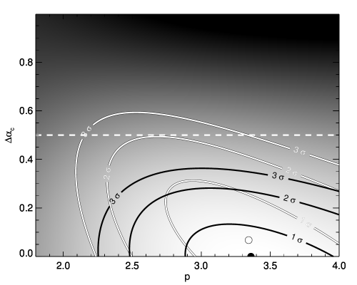
Figure 3: Chi-square map of the particle spectral index $p$ and synchrotron cooling break$\Delta\alpha_{\rm c}$, derived by fitting the “fundamental plane” radio-X-ray-mass correlation with cooled synchrotron emission as the source of the X-rays and a flat, optically thick radio synchrotron spectrum with index $\alpha_{\rm r}=0$. Over-plotted are the the 1, 2, and 3-sigma contours (thick black lines), the best fit (black dot), and the canonical cooling break of $\Delta\alpha_{\rm c}=1/2$ (white dashed line). A reasonable fit requires an unbroken, i.e. uncooled global spectrum that is steeper than $p\mathrel{\hbox{\hbox to0.0pt{\hbox{\lower 4.0pt\hbox{$\sim$}}\hss}\hbox{$>$}}}3$. Also shown are the same 1, 2, and 3 sigma contours and the best fit obtained by fitting only low-X-ray luminosity sources with $L_{\rm x}\leq 10^{-3}L_{\rm Edd}$ (white contours and white dot).

Merloni et al. (2003) and Maccarone et al. (2003) discuss the possibility that the radio-X-ray-mass correlation of the “fundamental plane” breaks down at high accretion rates and that different emission mechanisms are responsible for the X-rays above and below the break. However, repeating the analysis with a sample limited to low X-ray luminosities ($L_{\rm x}<10^{-3}L_{\rm Edd}$) does not change the conclusions reached above, only the confidence contours in Fig. 3 are slightly less stringent: $p=3.3^{+0.8}_{-0.6}$, $\Delta\alpha_{\rm x}=0.1^{0.2}_{-0.1}$, and $\alpha_{\rm x}=1.25^{+0.35}_{-0.3}$, as shown by the white contours in Fig. 3.

In fact, the X-ray spectra of the low luminosity sources (white dots in Fig. 2) tend to be flatter than those of the high luminosity sources (black dots). While all the observed spectral indices in Fig. 2 are from AGNs, the same is known to be the case in XRBs, which typically show harder spectra in their low luminosity state. Thus, most of the observed X-ray spectral indices of low luminosity sources are significantly flatter than the range in $\alpha_{\rm x}$ allowed by fitting the scaling relations for synchrotron jet X-rays to the low luminosity sources in the “fundamental plane” sample.

3.3 Discussion

This discrepancy between the correlation indices of the fundamental plane, the predicted scaling relations, and the actually observed X-ray spectra suggests several possible scenarios (not necessarily mutually exclusive):

3.3.1 Steep global spectra

Fig. 3 indicates that the fundamental plane relation is compatible with X-ray synchrotron emission if the underlying particle distribution is inherently steep, with $p\sim 3.3$. Such a steep, unbroken particle distribution can be achieved in two ways:

a) The particle acceleration process produces inherently steep spectra with $p\sim 3$ (unlike Fermi I acceleration), and radiative cooling is unimportant even at X-ray energies. However, for radiative cooling to have no effect, even on the X-ray emitting electrons, the magnetic fields in the inner jet would have to be very low.

b) Particle acceleration produces spectra close to $p\sim 2$, but radiative cooling steepens the spectra to an index of $p\sim 3$ all the way down below radio frequencies (in which case the formalism above cannot distinguish between cooling and an intrinsically steep spectrum). However, the jet is optically thick at lower frequencies. The cooling coefficient for electrons radiating below the self-absorption turnover frequency is significantly reduced (McCray, 1969; Ghisellini et al., 1988), and an unbroken powerlaw is not a solution to the kinetic equation in this case. The self-absorption barrier can be circumvented if radiation losses are dominated by inverse Compton scattering. A radiative signature of this component must be visible, since it would dominate the radiative output of the jet (presumably in the X-rays). Alternatively, a somewhat fine–tuned adiabatic loss scheme could keep the synchrotron cooling break always below the local turnover frequency.

However, such a steep global spectrum is inconsistent with the flatter radio spectral indices observed in larger scale optically thin jet sources (like M87, GRS 1915+105, 3C273, etc.) and would therefore require additional particle acceleration on larger spatial scales. It is also inconsistent with the standard scenario for producing flat radio spectra (Blandford & Ostriker, 1978). And for most sources in Fig. 2 (and XRBs in the low-hard state), the observed X-ray spectral indices $\alpha_{\rm x}$ are much shallower than this. Ultimately, broad band spectra of the jet core are necessary to verify the spectral index of the optically thin part of the spectrum over a large frequency range and for a number of sources with different $M$ and $\dot{m}$ to determine $p$ unequivocally.

3.3.2 Scale invariance violated

It is possible that the X-rays of all sources in the sample are of synchrotron–jet origin, but that jets are inherently not scale invariant and the analysis presented above and in Heinz & Sunyaev (2003) does not apply. However, the presence of a strong correlation and its agreement with the scale invariance predictions would be a coincidence. Moreover, specific models used by Markoff et al. (2001) and Markoff et al. (2003) (based on the original, scale invariant jet model by Blandford & Königl, 1979) and by Falcke & Biermann (1995), Markoff et al. (2003), and Falcke et al. (2004) to model the correlation and the broad band spectra of individual sources are themselves members of the class of scale invariant models. Such a lack of scale invariance would require a more complex approach at understanding jet spectra and correlations.

3.3.3 Other sources of X-ray emission

Finally, the discrepancy can be resolved if the X-ray emission from at least a significant fraction of the sources in the “fundamental plane” sample does not originate as synchrotron emission in the jet, but either a) in the disk, as long as the X-ray emission from the disk is inefficient in the sense that $F_{\rm x}\propto\dot{m}^{2}$, or b) as inverse Compton emission from the jet, with seed photons provided by the accretion flow, the jet radio synchrotron emission, or the companion (Georganopoulos et al., 2002; Markoff & Nowak, 2004).

The disk interpretation would be in line with the fact that the inefficient disk X-ray scenario provides the best global fit to the fundamental plane relation. Discussing the inverse Compton scenario is beyond the scope of this paper. It is clear, though, that the presence of the radio-X-ray-mass correlation will impose similar limits on a Compton scenario as is the case in disk X-rays (e.g., it might help us to determine the source of the up-scattered photons, i.e., disk vs. synchrotron-self-Compton). Clearly, further research is necessary to explore this scenario.

Given the large scatter in the fundamental plane relation, the X-rays of at least a part of the sample might still be predominantly jet–synchrotron emission. In fact, it is quite plausible to expect that all three emission mechanisms will make a contribution to the X-ray spectrum of any given source at some level. It might well be that in different sources, different X-ray emission mechanisms dominate, leading to the significant observed scatter in the “fundamental plane”. For example, the X-rays from Galactic XRBs in the low hard state might be of jet synchrotron origin, while the X-rays from AGNs might originate primarily in the disk (or vice versa). In this case, the fact that both XRBs and AGNs fall on the same relation would be a coincidence.

The scaling relations derived above and in Heinz & Sunyaev (2003); Falcke & Biermann (1995) can help to distinguish between these different types of sources in a large enough, well characterized sample, which is clearly a primary objective for future research in this area.

3.4 Caveats

Some caveats and sources of uncertainty should be kept in mind when interpreting these results:

a) The “fundamental plane” sample is a relatively diverse sample, containing several different types of AGNs, spanning a large range in accretion rate and black hole mass (see Merloni et al. 2003 for a detailed discussion of the properties of the sample), mostly for the sake of a large number of sources and for testing the universality of the correlation. This is in line with the suggestion from §3.3.3 that sources with different X-ray emission mechanisms may be present in the sample. Due to the diverse nature of the sample, some systematic effects may be present that we have not accounted for. In the context of this paper, however, a reduction to the more homogeneous low-luminosity sample (also used by Falcke et al. 2004) shows identical results.

b) The X-ray spectral characteristics of XRBs change as they change state, and the radio and X-ray band vary on different time scales and with respective phase lags. This specifically affects the global spectral index. The same should hold for AGNs, though it is difficult to test due to the long time scales involved. However, as long as there is a simple delay between the two bands and no systematic trend for one band (X-ray or radio) to be in a specific state longer than the other, the variability should average out in a large enough sample and be simply another source of scatter in the fundamental plane. The presence of the radio-X-ray correlation in XRBs in GX 339-4 (Corbel et al., 2003) and V404 Cyg (Gallo et al., 2003) indicates that variability effects do not destroy the correlation at least in the case of XRBs. It has to be kept in mind that the error bars on some of the $\alpha_{\rm x}$ measurements from the literature shown in Fig. 2 are very large. Clearly, future observations with tighter error bars will be very helpful to strengthen the arguments made in this paper.

c) The same holds for the radio spectral index: it is known that as a the source flux changes in XRBs, $\alpha_{\rm r}$ also varies by significant amounts. However, at least for AGNs we know that, on average, a flat spectrum is a good description of the radio core, and while the situation for XRBs at very low luminosities should be explored further, it is probably a good approximation to assume that the spectra are, on average, close to flat (Fender, 2001). Again, the radio-X-ray correlation indicates that the underlying spectrum is unlikely to vary randomly, since the radio-X-ray correlation would otherwise be a coincidence.

Thus, while we expect all of these effects to be present and to be important on a detailed, quantitative level, we believe that they do not alter the fundamental presence of the correlation and that we can use a statistical approach (i.e., measuring the correlation coefficient) to learn something about the underlying nature of the emitter. However, all of these effects will contribute to the scatter and the uncertainty in any conclusion and must therefore be better characterized in future studies.

4 Conclusions

We presented an extension of the scale invariance formalism derived by Heinz & Sunyaev (2003) that takes the effects of radiative cooling into account self-consistently. The spectral index information of the sources contributing to the “fundamental plane” correlation shows that the X-ray luminosity of the sources should be affected by cooling if it is due to synchrotron emission from the jet. We proved that, for the canonical synchrotron parameters ($p=2$, $\Delta\alpha=1/2$), the scaling relations for X-ray and radio synchrotron emission cannot reproduce the correlation coefficients found by Merloni et al. (2003).

Fitting the newly derived scaling relations to the fundamental plane data, we showed that steep ($p\sim 3.4$, $\alpha_{\rm x}\sim 1.2$), unbroken spectra are required to reproduce the correlation coefficients. Such steep spectra are inconsistent with the observed mean and median spectral index of the “fundamental plane” sources with measured spectra. This seeming discrepancy leads us to propose three alternative scenarios: a) The X-rays are of synchrotron origin and the entire electron spectrum has a steep index of order $\sim 3$, which would require steep injection spectra or inverse Compton cooling of the entire powerlaw distribution of electrons to well below radio frequencies. However, such steep spectra are inconsistent with the observed range in X-ray spectral indices $\alpha_{\rm x}$; b) the X-rays are due to synchrotron emission from jets, but some of the assumptions made in deriving the scale invariance predictions fail (i.e., some aspect of jet dynamics is not scale invariant); c) the X-rays from a sizeable fraction of the sources in the sample are not of jet-synchrotron origin and are thus most likely emitted either by the accretion flow itself or as Compton up-scattered radiation from the jet. It still plausible that a fraction of the sources (e.g., most of the XRBs) in the sample emit predominantly synchrotron X-rays and that synchrotron emission from jets contributes a small fraction to the X-ray spectrum of most sources.

The analysis presented in this paper shows how a statistical analysis of radio and X-ray luminosities of a sample of black holes can be used to constrain the X-ray emission mechanism of accreting black holes and to test the scale invariance hypothesis of jets. A more refined sample of black holes with a better understanding of the sources of scatter (and the selection effects involved), and with tighter limits on the X-ray spectral indices is necessary to take this analysis to a more precise quantitative level.

We would like to thank Sera Markoff, Andrea Merloni, Mike Nowak, and Rashid Sunyaev for helpful discussions. Support for this work was provided by the National Aeronautics and Space Administration through Chandra Postdoctoral Fellowship Award Number PF3-40026 issued by the Chandra X-ray Observatory Center, which is operated by the Smithsonian Astrophysical Observatory for and on behalf of the National Aeronautics Space Administration under contract NAS8-39073.

Appendix A Full derivation of the scaling relations

A.1 Particle transport

In this appendix, we will derive the scaling relations for X-ray synchrotron radiation from scale invariant jets, including radiative cooling. We refer the reader to §2 for the set of assumptions going into the scale invariance ansatz. Again, we assume that the particles are injected into the jet at some scale invariant location $r_{0}$ and time $t_{0}$ (the latter measured in the jet frame).

The kinetic equation describing the evolution of the particle distribution function $f(\gamma)$ as a function of time $t$ and particle energy $\gamma$ is (adapted from Coleman & Bicknell, 1988):

$$\frac{\partial f}{\partial t}+\frac{d\ln{(\rho)}}{dt}\left[\frac{\gamma^{3}}{3}\frac{\partial}{\partial\gamma}\left(\gamma^{-2}f\right)\right]=\frac{2e^{4}\langle B_{\perp}^{2}\rangle}{3m_{\rm e}^{3}c^{5}}\frac{\partial{\left(\gamma^{2}f\right)}}{\partial\gamma}$$ (18)

where an isotropic pitch angle distribution of the particles was assumed for the numerical coefficients (this assumption is not critical for the derivation, since the relevant numerical coefficients don’t enter into the scaling relations). Eq. (18) can be easily expanded to include inverse Compton losses by adding a term proportional to the radiation energy density to the right hand side of eq. (18).

For mathematical convenience, we substitute

$$\hat{\gamma}\equiv\left(\rho_{0}/\rho\right)^{1/3}\gamma$$ (19)

where $\rho_{0}\equiv\rho(t_{0})$ is the density at the point $\chi_{0}=r_{0}/r_{\rm g}$ where the particles were accelerated/injected, and $\tilde{t}\equiv t/t_{0}$ is the time when the particles are injected (measured in the jet frame). We also substitute $\tilde{f}\equiv\left(\rho/\rho_{0}\right)^{-2/3}f$.

As plasma travels along the jet, there is a one-to-one relation between its jet coordinate $\chi$ and the time $\tilde{t}$, defined by

$$\frac{d\chi}{d{\tilde{t}}}=\frac{t_{0}}{r_{\rm g}}{c\beta\Gamma}=\frac{t_{0}c}{r_{\rm g}}{\psi_{\beta\Gamma}(\chi)}$$ (20)

We define $\chi_{0}$ as the acceleration location such that ${\tilde{t}}(\chi_{0})=1$. By virtue of the assumption that the particle injection location is scale invariant, this value of $\chi_{0}$ must be independent of $M$ and $\dot{m}$. We can then substitute the integration over $\tilde{t}$ by one over $\chi$.

The characteristic equation for synchrotron and adiabatic losses for each particle implicit in eq. (18) is:

$$\frac{d\hat{\gamma}}{d\chi}=-{A_{0}}\frac{1}{\psi_{\beta\Gamma}(\chi)}\left(\frac{B}{B_{0}}\right)^{2}\left(\frac{\rho}{\rho_{0}}\right)^{1/3}{\hat{\gamma}}^{2}$$ (21a)

$$= -{A_{0}}\left[\psi_{\beta\Gamma}(\chi)\right]^{-1}\left[\psi_{B}(\chi)\right]^{2}\left[\psi_{\rho}(\chi)\right]^{1/3}{\hat{\gamma}}^{2}$$ (21b)

$$A_{0} \equiv r_{g}{\phi_{B}}^{2}\frac{4e^{4}}{9m^{3}c^{6}}$$ (21c)

where we used eq. (1) in the last step.

Equation (21a) has the solution

$$\hat{\gamma}(\chi)=\frac{1}{\frac{1}{{\hat{\gamma}}_{0}}+A_{0}\int_{\chi_{0}}^{\chi}d{\chi}^{\prime}\frac{\left[\psi_{B}(\chi^{\prime})\right]^{2}\left[\psi_{\rho}(\chi^{\prime})\right]^{\frac{1}{3}}}{\left[\psi_{\beta\Gamma}(\chi^{\prime})\right]}}$$ (22)

where ${\hat{\gamma}}_{0}\equiv\gamma(t_{0})$. For convenience we define

$${\xi(\chi)} = \frac{A_{0}\int_{\chi_{0}}^{\chi}d\chi^{\prime}\left[\psi_{\beta\Gamma}(\chi^{\prime})\right]^{-1}\left[\psi_{B}(\chi^{\prime})\right]^{2}\left[\psi_{\rho}(\chi^{\prime})\right]^{1/3}}{\left[\psi_{\rho}(\chi)\right]^{\frac{1}{3}}}$$ (23a)

$$= \phi_{\xi}(M,\dot{m})\psi_{\xi}(\chi)$$ (23b)

where, by definition,

$$\phi_{\xi}(M,\dot{m})=M\left[{\phi_{B}(M,\dot{m})}\right]^{2}$$ (24)

and $\psi_{\xi}$ is independent of $M$ and $\dot{m}$ (but might have an implicit dependence on parameters such as black hole spin). $\xi$ is simply the inverse of the synchrotron cutoff energy, $\xi=1/\gamma_{\rm c}$, while $\phi_{\xi}$ describes how this energy cutoff in the electron spectrum depends on $M$ and $\dot{m}$.

We can then solve eq. (18) along the characteristics defined by eq. (22), which reduces the problem to an ODE:

$$\frac{d\left\{\left[{\hat{\gamma}}(\chi)\right]^{2}\tilde{f}\left[\hat{\gamma}(\chi)\right]\right\}}{d\chi}=0$$ (25)

where $d/d\chi$ is the total derivative along curves $\hat{\gamma}(\chi)$ defined by eq. (22). In other words, the function ${\hat{\gamma}}^{2}\tilde{f}$ is constant along solutions of eq. (21a). The well known solution to eq. (18) is then (Kardashev, 1962; Bicknell & Melrose, 1982):

$$f(\gamma,\chi)=\left(\frac{\left[\psi_{\rho}(\chi)\right]^{-\frac{1}{3}}{\gamma}}{1-\xi\gamma},\chi_{0}\right)\left(1-\xi{\gamma}\right)^{-2}\left[\psi_{\rho}(\chi)\right]^{\frac{2}{3}}$$ (26)

for $\gamma\leq\gamma_{\rm c}\equiv 1/\xi$ and the solution has a cutoff at $\gamma_{\rm c}$ such that $f(\gamma>\gamma_{\rm c},t)=0$. For later use, we define the scaled Lorentz factor as the ratio of the particle energy to this cutoff:

$$\tilde{\gamma}\equiv\gamma\xi=\frac{\gamma}{\gamma_{\rm c}}$$ (27)

Using the assumption that the injected particle distribution at $\chi_{0}$ is a powerlaw as described in eq. (2), we can write $f(\gamma,\chi)$ as

$$f(\gamma,\chi)=\phi_{C}\xi^{p}{\hat{\gamma}}^{-p}\left(1-\hat{\gamma}\right)^{p-2}\left[\psi_{\rho}(\chi)\right]^{(p+2)/3}$$ (28)

A.2 Synchrotron emission from cooled particle distributions

Following the notation in Rybicki & Lightman (1979), we define the critical synchrotron frequency as

$$\nu_{\rm c}(\gamma) \equiv \frac{3e}{16mc}B\gamma^{2}$$ (29)

(where we have averaged over the assumed isotropic pitch angle distribution – as before, this assumption is not critical for the derivation below). This is the frequency where most of the energy of the synchrotron kernel is emitted for an electron of energy $\gamma m_{e}c^{2}$.

The synchrotron luminosity $F_{\nu}$ at frequency $\nu$ is then

$$F_{\nu}=$$ (30)

$$\ \ \ \ \ \int_{r(t_{0})}^{\infty}dr\pi R_{\rm jet}^{2}\frac{\sqrt{3}e^{3}B\langle sin{\alpha}\rangle}{m_{\rm e}c^{2}}\int_{\gamma_{\rm min}}^{\gamma_{\rm c}}d\gamma f(\gamma){\rm F_{s}}\left(\frac{\nu}{\nu_{c}(\gamma)}\right)$$

where

$${\rm F_{s}}(x)\equiv x\int_{x}^{\infty}dx^{\prime}{\rm K_{5/3}}(x^{\prime})$$ (31)

is the synchrotron kernel. Substituting the expressions from eq. (28) and eq. (1) we get

$$F_{\nu}=M^{3}\phi_{B}\phi_{C}{\phi_{\xi}}^{p-1}F_{0}\int_{\chi_{0}}^{\infty}d\chi\left[\psi_{B}\psi_{R}^{2}\psi_{\rho}^{(p+2)/3}\psi_{\xi}^{p-1}\raisebox{12.0pt}[12.0pt][12.0pt]{\ }\right.$$

$$\hskip 130.08731pt\left.\raisebox{12.0pt}[12.0pt][12.0pt]{\ }\int_{0}^{1}d{\tilde{\gamma}}\ {\tilde{\gamma}}^{-p}\left(1-\tilde{\gamma}\right)^{p-2}{\rm F}\left(\frac{\tilde{\nu}{\psi_{\xi}}^{2}}{\psi_{B}{\tilde{\gamma}}^{2}}\right)\right]$$

where we have defined

$$\tilde{\nu}\equiv\frac{16m_{\rm e}c}{3e}\frac{\nu\,{\phi_{\xi}}^{2}}{\phi_{B}}$$ (33)

and

$$F_{0}\equiv\frac{\pi^{2}\sqrt{3}e^{3}}{4m_{\rm e}c^{2}}$$ (34)

(where we have taken the magnetic field to be isotropically tangled, without loss of generality).

Before progressing further, it is important to note several things about eq. (A.2)

• The low energy cutoff enters into the boundaries of the integral over $\tilde{\gamma}$. However, since we are dealing with optically thin synchrotron radiation at high frequencies (X-rays), the low energy cutoff has a negligible effect on the integral, since the synchrotron kernel drops exponentially at low particle energies and the integral converges even if the lower bound is placed at zero, which we have done in eq. (A.2).

• As a function of $\tilde{\nu}$, the integrand is entirely independent of $M$ and $\dot{m}$, which enter only into $\phi_{B}$, $\phi_{C}$, and $\phi_{\xi}$ in front of the integral. However, $\tilde{\nu}$ does depend on $M$ and $\dot{m}$ through $\phi_{B}$ and $\phi_{C}$.

• As discussed earlier, $\phi_{B}$ and $\phi_{C}$ are simply the magnetic field strength $B$ and the normalization $C$ of the particle distribution at the base of the jet (both of which vary with $M$ and $\dot{m}$), whereas $\phi_{\xi}$ describes how the cutoff energy $\gamma_{\rm c}$ at a given position $\chi$ depends on $M$ and $\dot{m}$, as defined in eq. (24). The fact that we can write down a simple dependence of $\gamma_{\rm c}$ on $M$ and $\dot{m}$ will allow us below to set the cooled synchrotron flux in relation to $M$ and $\dot{m}$ as well.

Following the same procedure as Heinz & Sunyaev (2003), we are now in a position to derive the scaling relation between the synchrotron flux at X-ray energies $F_{\nu}$ and $M$:

$$\frac{\partial\log{F_{\nu}}}{\partial\log{M}}=\frac{\partial\log{\left(M^{3}\phi_{B}\phi_{C}\phi_{\xi}^{p-1}\right)}}{\partial\log{M}}+\frac{\partial\log{F_{\nu}}}{\partial\log{\tilde{\nu}}}\frac{\partial\log{\tilde{\nu}}}{\partial\log{M}}$$ (35)

$$= 2-2\alpha_{\rm x}+p+\frac{\partial\log{(\phi_{C}})}{\partial\log{M}}+(2p-1-3\alpha_{\rm x})\frac{\partial\log{(\phi_{B})}}{\partial\log{M}}$$

$$\equiv \xi_{\rm xM}$$

where we used the X-ray spectral index $\alpha_{\rm x}$ such that $F_{\rm x}\propto\nu^{-\alpha_{\rm x}}$ or $\alpha_{\rm x}\equiv-\frac{\partial\log{F_{\nu}}}{\partial\log{\nu}}$.

Note that eq. (8) is fully general as long as synchrotron self-absorption is negligible, even in the absence of any cooling. This can be checked by comparing this eq. (8) to the equivalent expression in Heinz & Sunyaev (2003) by substituting $\alpha_{\rm x}=(p-1)/2$, which is the appropriate expression of optically thin, uncooled synchrotron emission.

Similarly, we can derive the scaling relation between $F_{\nu}$ and the accretion rate $\dot{m}$:

$$\frac{\partial\log{F_{\nu}}}{\partial\log{\dot{m}}}=\frac{\partial\log{\left(M^{3}\phi_{B}\phi_{C}\phi_{\xi}^{p-1}\right)}}{\partial\log{\dot{m}}}+\frac{\partial\log{F_{\nu}}}{\partial\log{\tilde{\nu}}}\frac{\partial\log{\tilde{\nu}}}{\partial\log{\dot{m}}}$$ (36)

$$= \frac{\partial\log{(\phi_{C}})}{\partial\log{\dot{m}}}+(2p-1-3\alpha_{\rm x})\frac{\partial\log{(\phi_{B})}}{\partial\log{\dot{m}}}\equiv\xi_{\rm x\dot{m}}$$

$\dot{m}$ is simply a parameter describing the variation of magnetic field and particle pressure at the base of the jet at constant $M$, and must not necessarily be directly proportional to the accretion rate. These two equations are the scaling laws used throughout this paper

The superposition of cooled electron spectra from different regions in the jet might, in principle, produce any number of spectral shapes (e.g., broken powerlaws, cutoff, curved spectra, etc.). Eqs. (8) and (9), as derived in the appendix, are independent of what the actual X-ray spectral shape is. However, observations of synchrotron spectra from sources where we know cooling is efficient show either exponential-type cutoffs or, if fresh plasma is continuously supplied, broken powerlaw spectra. The latter case is appropriate here, since we are observing a superposition of spectra from plasma that moves away from a stationary or quasi-stationary acceleration region. Therefore, we can expect the cooled X-ray spectrum to be of powerlaw type:

$$F_{\rm x}\propto M^{\xi_{rmxM}}{\dot{m}}^{\xi_{\rm x\dot{m}}}$$ (37)

A.3 Inverse Compton cooling

It is easy to change the cooling mechanism in eq. (18) to inverse Compton cooling off of radiation from either the central accretion disk or the microwave background. The latter will be entirely irrelevant in the context of core dominated jets and we will ignore it in the following paragraph. The former can be included by substituting $8\pi\,U_{\rm rad}$ for ${B_{\perp}}^{2}$ in eq. (18). In this case the function $\phi_{\xi}$ will have to be changed to reflect the dependence of the radiation energy density on $M$ and $\dot{m}$, which depends on the accretion scenario. In the case of an efficient accretion disk with $\phi_{\rm B}=\sqrt{\dot{m}/M}$, we have

$$\phi_{\xi}\propto r_{\rm g}M^{-1}\dot{m}$$ (38)

which has exactly the same dependence on $M$ and $\dot{m}$ as in the synchrotron loss case, and the solution is unchanged. In radiatively inefficient flows, we have approximately

$$\phi_{\xi}\propto r_{\rm g}M^{-1}{\dot{m}}^{2}$$ (39)

which implies that inverse Compton is increasingly unimportant compared to synchrotron cooling at low accretion rates. It also implies that, while $\xi_{\rm xM}$ is unchanged, $\xi_{{\rm x}\dot{m}}$ is changed to

$$\xi_{{\rm x}\dot{m}}=2p-1/2-3\alpha_{\rm x}$$ (40)

References

- Achterberg et al. (2001) Achterberg, A., Gallant, Y. A., Kirk, J. G., & Guthmann, A. W. 2001, MNRAS, 328
- Bell (1978) Bell, A. R. 1978, MNRAS, 182, 147
- Bicknell & Melrose (1982) Bicknell, G. V. & Melrose, D. B. 1982, ApJ, 262, 511
- Blandford & Begelman (1999) Blandford, R. D. & Begelman, M. C. 1999, MNRAS, 303, L1
- Blandford & Königl (1979) Blandford, R. D. & Königl, A. 1979, ApJ, 232, 34
- Blandford & Ostriker (1978) Blandford, R. D. & Ostriker, J. P. 1978, ApJL, 221, L29
- Coleman & Bicknell (1988) Coleman, C. S. & Bicknell, G. V. 1988, MNRAS, 230, 497
- Corbel et al. (2003) Corbel, S., Nowak, M. A., Fender, R. P., Tzioumis, A. K., & Markoff, S. 2003, A&A, 400, 1007
- Drury et al. (1982) Drury, L. O., Axford, W. I., & Summers, D. 1982, MNRAS, 198, 833
- Falcke & Biermann (1995) Falcke, H. & Biermann, P. L. 1995, A&A, 293, 665
- Falcke et al. (2004) Falcke, H., Körding, E., & Markoff, S. 2004, A&A, 414, 895
- Fender (2001) Fender, R. P. 2001, MNRAS, 322, 31
- Fossati et al. (1998) Fossati, G., Maraschi, L., Celotti, A., Comastri, A., & Ghisellini, G. 1998, MNRAS, 299, 433
- Gallant et al. (1999) Gallant, Y. A., Achterberg, A., & Kirk, J. G. 1999, A&AS, 138, 549
- Gallo et al. (2003) Gallo, E., Fender, R. P., & Pooley, G. G. 2003, MNRAS, 344, 60
- Gebhardt et al. (2000) Gebhardt, K., Bender, R., Bower, G., Dressler, A., Faber, S. M., Filippenko, A. V., Green, R., Grillmair, C., Ho, L. C., Kormendy, J., Lauer, T. R., Magorrian, J., Pinkney, J., Richstone, D., & Tremaine, S. 2000, ApJL, 539, L13
- Georganopoulos et al. (2002) Georganopoulos, M., Aharonian, F. A., & Kirk, J. G. 2002, A&A, 388, L25
- Ghisellini et al. (1988) Ghisellini, G., Guilbert, P. W., & Svensson, R. 1988, ApJL, 334, L5
- Heinz & Sunyaev (2002) Heinz, S. & Sunyaev, R. 2002, A&A, 390, 751
- Heinz & Sunyaev (2003) Heinz, S. & Sunyaev, R. A. 2003, MNRAS, 343, L59
- Jester et al. (2001) Jester, S., Röser, H.-J., Meisenheimer, K., Perley, R., & Conway, R. 2001, A&A, 373, 447
- Kardashev (1962) Kardashev, N. S. 1962, Soviet Astronomy, 6, 317
- Larrabee et al. (2003) Larrabee, D. A., Lovelace, R. V. E., & Romanova, M. M. 2003, ApJ, 586, 72
- Maccarone et al. (2003) Maccarone, T. J., Gallo, E., & Fender, R. 2003, MNRAS, 345, L19
- Markoff et al. (2001) Markoff, S., Falcke, H., & Fender, R. 2001, A&A, 372, L25
- Markoff & Nowak (2004) Markoff, S. & Nowak, M. 2004, accepted for publication in ApJ
- Markoff et al. (2003) Markoff, S., Nowak, M., Corbel, S., Fender, R., & Falcke, H. 2003, A&A, 397, 645
- McCray (1969) McCray, R. 1969, ApJ, 156, 329
- Merloni & Fabian (2002) Merloni, A. & Fabian, A. C. 2002, MNRAS, 332, 165
- Merloni et al. (2003) Merloni, A., Heinz, S., & di Matteo, T. 2003, MNRAS, 345, 1057
- Narayan et al. (2000) Narayan, R., Igumenshchev, I. V., & Abramowicz, M. A. 2000, ApJ, 539, 798
- Narayan & Yi (1994) Narayan, R. & Yi, I. 1994, ApJL, 428, L13
- Quataert & Gruzinov (2000) Quataert, E. & Gruzinov, A. 2000, ApJ, 539, 809
- Rybicki & Lightman (1979) Rybicki, G. B. & Lightman, A. P. 1979 (New York: Wiley)
- Sams et al. (1996) Sams, B. J., Eckart, A., & Sunyaev, R. 1996, Nature, 382, 47
- Shakura & Sunyaev (1973) Shakura, N. I. & Sunyaev, R. A. 1973, A&A, 24, 337
- Shapiro et al. (1976) Shapiro, S. L., Lightman, A. P., & Eardley, D. M. 1976, ApJ, 204, 187