Noise in strong lensing cosmography

Abstract

Giant arcs in strong lensing galaxy clusters can provide a purely geometric determination of cosmological parameters, such as the dark energy density and equation of state. We investigate sources of noise in cosmography with giant arcs, focusing in particular on errors induced by density fluctuations along the line-of-sight, and errors caused by modeling uncertainties. We estimate parameter errors in two independent ways, first by developing a Fisher matrix formalism for strong lensing parameters, and next by directly ray-tracing through N-body simulations using a multi-plane lensing code. We show that for reasonable power spectra, density fluctuations from large-scale structure produce $>100\%$ errors in cosmological parameters derived from any single sightline, precluding the use of individual clusters or “golden lenses” to derive accurate cosmological constraints. Modeling uncertainties similarly can lead to large errors, and we show that the use of parametrized mass models in fitting strong lensing clusters can significantly bias the inferred cosmological parameters. We lastly speculate on means by which these errors may be corrected.

1. Introduction

There is strong observational evidence supporting the flat $\Lambda$CDM cosmological model, in which the energy budget of the universe is dominated by a poorly understood dark sector (e.g Bennett et al., 2003; Riess et al., 2004). An important question is whether dark energy, which comprises at present $\Omega_{\Lambda}\approx 0.7$ of the critical density, is truly a cosmological constant or instead a dynamical field with evolving energy density. Considerable effort has been directed towards developing means of measuring the redshift evolution of dark energy, and one of the most promising methods involves gravitational lensing tomography. The basic idea is to exploit the fact that the lensing efficiency for a lens at distance $D_{l}$ and source at $D_{s}$ is proportional to $D_{l}\,D_{ls}/D_{s}$. By measuring the variation of lensing strength with source redshift, one can measure distance ratios as a function of redshift, and thereby constrain the background cosmology. Tomographic weak lensing is also sensitive to the growth of structure, providing an additional handle on dark energy (e.g. Hu, 2002), although it may be possible to separate the effects of growth and geometry in weak lensing tomography (Jain & Taylor, 2003; Zhang et al., 2003) if a purely geometric determination of the cosmology is desired.

This method may also be applied in the strong lensing regime (e.g. Blandford & Narayan, 1992). Golse et al. (2002) discuss in detail the cosmographic prospects for a sample of galaxy clusters, each with multiple giant arcs at different redshifts, and Soucail et al. (2004) apply this method to the galaxy cluster Abell 2218 to derive preliminary cosmological constraints. Cluster surveys, such as the MACS survey (Ebeling et al., 2001), EDisCS survey (Gonzalez et al., 2002), or SDSS cluster lensing survey (Hennawi et al., 2004), and wide-area imaging surveys like the CFHT Legacy Survey or the RCS-2 survey are expected to find (and are finding!) large numbers of arc-bearing galaxy clusters. Frequently, deep imaging reveals multiple arcs in the same cluster – a spectacular example is provided by Abell 1689 (Benítez et al., 2002a). With this imminent explosion in strong lensing data, it is now appropriate to consider realistic sources of noise in lensing cosmography, with an aim towards determining optimal observational strategies. For example, is it better to devote large amounts of telescope time to a few clusters, in the hopes of finding dozens of arcs per cluster which completely constrain the mass model, or is it better to survey a large number of clusters and study only a few arcs per cluster?

In this paper, we study two principal sources of noise in strong lensing cosmography. First, we consider how uncertainties in the mass modeling of the lensing cluster translate into errors in the derived cosmological parameters. Next, we investigate the effects of random density fluctuations in the line of sight uncorrelated with the main lensing cluster. We find that density fluctuations can lead to large errors in the inferred cosmology along any given sightline. This requires the use of multiple sightlines; that is many lensing clusters must be studied in order to suppress the noise associated with large-scale structure. With limited telescope time, this may also lead to problems: the limited constraints provided by small numbers of arcs per cluster require the use of parametric mass models in fitting the lens data, and we show that such parametric models can produce biases in the inferred cosmological parameters.

2. Sources of noise

It is perhaps worth emphasizing the well-known point that determining the properties of dark energy using gravitational lensing tomography is quite difficult, because variation of dark energy parameters produces small effects on the lensing observables. For tomographic lensing, the basic observable is the variation of lensing efficiency $G\propto D_{l}\,D_{ls}/D_{s}$ with source redshift. We do not measure the absolute lensing efficiency, only the ratio of efficiencies at different redshifts. In figure 1 we plot the ratio $G(z)/G(1)$ for lens redshift $z_{l}=0.3$, as a function of source redshift $z$ for several values of $w$. As can be seen, in order to produce interesting constraints on $w$ we must be able to measure the lensing efficiency at the percent level, which is quite challenging. Weak lensing surveys aim to overcome this challenge using brute force, by surveying large fractions of the sky and measuring ellipticities of huge numbers of galaxies. Because strong lensing events are rare, it would be desirable to focus instead on a small number of objects and study them well. The fact that the signal is so small, however, means that strong lensing cosmography will be subject to a wide variety of error sources.

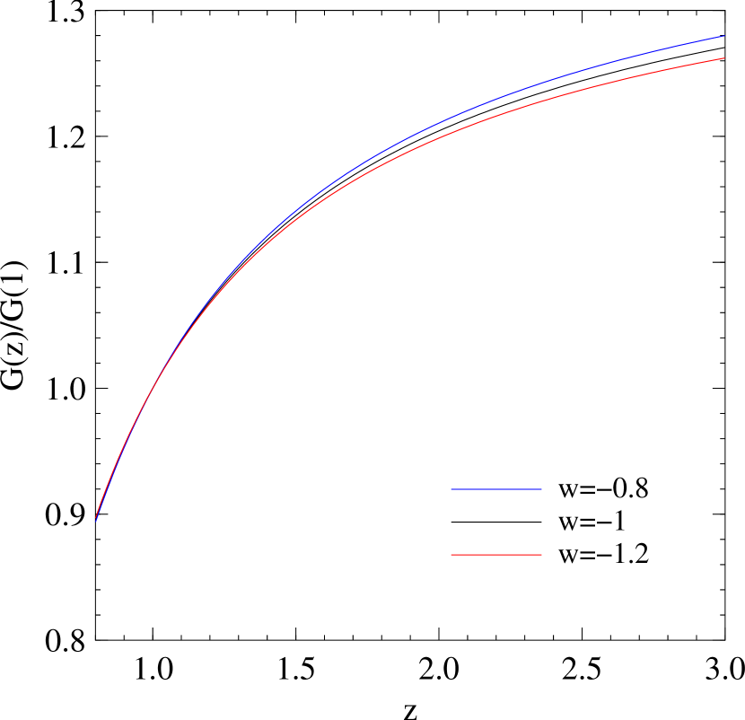
Figure 1.— Ratio of lensing efficiency, $G(z)/G(1)$, as a function of redshift. The curves correspond to dark energy equation of state parameter $w=-0.8,\,-1,\,-1.2$ from top to bottom.

2.1. Uncertainties in mass modeling

Uncertainties in mass modeling have long impeded the cosmographic applications of strong lenses. For example, the main systematic uncertainty in determination of the Hubble constant $H_{0}$ using lens time delays continues to be the radial density profile of the lens (e.g. Kochanek, 2002). Similarly, uncertainties in the mass modeling of lensing clusters also induce errors in the inferred cosmology. The reason is easy to understand – variations in the dark energy evolution, which change $\Sigma_{\rm crit}(z)$, can be compensated by adjusting the model density profile $\Sigma(R)$ to hold fixed the observables, which depend only upon the ratio $\Sigma/\Sigma_{\rm crit}$.

In the appendix, we calculate the parameter errors expected given a lens model and a specified level of observational errors. As shown in Appendix A, we can write the Fisher matrix as a sum over Fisher matrices for individual sources,

$${\bf F}_{\rm tot}=\int dz_{\rm src}\,n(z_{\rm src})\int d^{2}\!u\,{\bf F}(\bm{u},z_{\rm src}).$$ (1)

Here, $n(z_{\rm src})$ describes the number density of sources as a function of redshift $z_{\rm src}$, and the integral over source position $\bm{u}$ is restricted to the strong lensing region at each redshift. To illustrate the level of errors expected, let us consider strong lensing by two classes of models: an ellipsoidal NFW (Navarro et al., 1997) model, and the power-law ellipsoid model of Barkana (1998). We additionally allow parameters for external shear, along with the cosmological parameters (here taken to be only $\Omega_{M}$ and $w$), all of which must be simultaneously determined from the image data. Assume that there are $N$ multiply imaged sources used to constrain the model, drawn from a population following a redshift distribution $n(z)\propto z^{2}\exp(-(z/z_{w})^{2})$ (Hu & Jain, 2003) over a range $0.8<z_{\rm src}<4$, with median redshift $z_{\rm med}=1.5$. Unless stated otherwise, we will assume for the underlying cosmology a flat $\Lambda$CDM model with WMAP parameters (Bennett et al., 2003): $\Omega_{M}=0.27$, $\Omega_{\Lambda}=0.73$, $\Omega_{B}h^{2}=0.024$, $h=0.72$, $n=1$, $\sigma_{8}=0.9$.

We first consider cosmological constraints from power-law ellipsoids. The fiducial parameter values we adopt for this lens model are: Einstein radius $b=10\arcsec$ (for $z_{\rm src}=4$), axis ratio $q=0.7$, isothermal profile, vanishing core radius, no external shear, and $\Omega_{M}=0.27$, $w=-1$. For concreteness, we take observational errors of $\sigma=0.1\arcsec$, appropriate for Hubble Space Telescope imaging. Ignoring the degeneracies between the cosmological parameters $(\Omega_{M},w)$ and the lens parameters we would obtain errors $\sigma_{\Omega}=0.07N^{-1/2}$ and $\sigma_{w}=0.1N^{-1/2}$ with $N$ arcs. However, marginalizing over the lens parameters, these errors explode up to $\sigma_{\Omega}=3.6N^{-1/2}$ and $\sigma_{w}=5N^{-1/2}$.

Next we consider the NFW model. One qualitative difference between this model and the singular isothermal ellipsoid is that the NFW profile produces a central image at small radii. This increases the dynamic range of the lensing constraints, and helps break degeneracies between the cosmology and the mass profile. Using fiducial NFW parameters of $M_{\rm vir}=5\times 10^{14}h^{-1}M_{\odot}$, $c_{\rm vir}=5$, axis ratio $q=0.7$ and no external shear, we find improved constraints: $\sigma_{\Omega}=0.5N^{-1/2}$, $\sigma_{w}=0.7N^{-1/2}$. The improvement can be explained in part by the extra constraints from the central image, and in part by the smaller number of parameters in the NFW model compared to the power-law ellipsoid.

In reality, central images are rarely detected in strong lenses, and are strongly affected by the properties of the central cD galaxy in the cluster. Additionally, we expect real clusters to exhibit a broader range of density profiles than can be accommodated by the NFW model, due to, for example, the effect of baryons. We therefore expect the errors in real clusters to be significantly larger than the errors we have computed for NFW ellipsoids. Note that these errors are only those caused by propagating the observational uncertainties; below we discuss additional sources of error. Already, though, these error levels would require large numbers of arcs in a given cluster for useful constraints to be placed on dark energy.

2.2. Systematic errors in the mass model

One reason for the large errors found above is that we employed models with many parameters, producing degeneracies with the cosmological parameters. This requires large numbers of arcs in order to constrain the model parameters sufficiently. Had we taken a less flexible model, we would not have found as large errors on the cosmological parameters. Unfortunately, real clusters are expected to exhibit a broad range of behavior, as found in N-body simulations. If the assumed mass model does not fully capture the range of behavior of the real density profile, then the derived cosmological parameters will be biased; that is, the fit can be improved by adjusting the cosmology to make the convergence $\kappa(R,z_{s})$ a better fit to the density profile than variations of the mass model $\Sigma(R)$ can accomplish alone.

This bias is illustrated in figure 2. The figure shows results of a Monte Carlo calculation, in which artificial arcs are generated using ellipsoidal NFW profiles, and fitted using softened power-law ellipsoidal models (Barkana, 1998), which can mimic a wide range of radial profiles over the relevant radii of interest for strong lensing. A CMB prior on the $\Omega_{M}-w$ plane has also been imposed: the distance to the last scattering surface at $z=1089$ is required to be $d_{A}=14\pm 0.2$ Gpc for $h=0.71$ (Bennett et al., 2003); the degenerate direction is along decreasing $w$ (i.e. more negative) as $\Omega_{M}$ is increased. For each realization, we generate 10 arcs each at redshifts of $z_{\rm src}=0.8$, 1.6, 2.4, 3.2 and 4 using the same NFW model, and fit all 50 arcs using the power-law ellipsoid model, allowing $\Omega_{M}$ and $w$ to vary in the fit. We plot only the best-fitting $\Omega_{M}$ and $w$ for each realization; although the confidence region for each realization is large, we can detect parameter biases by examining the best-fitting models. Clearly, the cosmological parameters derived from multiple arcs can be biased at significant levels (in this example, $\Delta w\sim 1$). The sign and direction of the bias depend upon the profile shapes for the cluster and the model, and could be different from cluster to cluster if there is significant variation among cluster profiles. The bias can be suppressed by using more flexible models in the fits. Unfortunately, as discussed above, extra degrees of freedom in the mass model come at the expense of weaker constraints on cosmology.

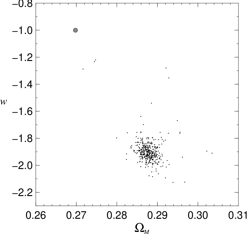
Figure 2.— Fits of NFW lenses to softened power-law ellipsoidal models. Each point corresponds to the best-fit values of $\Omega_{M}$ and $w$ derived by modeling sets of 50 randomly generated arcs at 5 different redshifts. The input cosmology had $\Omega_{M}=0.27$ and $w=-1$, as depicted by the filled circle.

2.3. Projection noise

In addition to the modeling uncertainties discussed above, another source of noise in strong lensing cosmography is large-scale structure. Fluctuations in the density along the line of sight, if uncorrected, produce errors in the derived cosmological parameters. Again, this effect is easy to understand – density fluctuations at redshifts different than the primary lens redshift have different lensing efficiencies than the primary lens, producing effects varying with source redshift which appear similar to variations in the background cosmology. Naively, one might expect the parameter errors to be small – the density fluctuations are at the $\lesssim 1\%$ level, and geometric factors suppress the effects of fluctuations at redshifts very different from the cluster redshift.

In the appendix, we compute the errors expected in the cosmological parameters caused by density fluctuations along the line of sight. We use the same fiducial lens models as in section §2.1, and estimate the line-of-sight density fluctuations by projecting the matter power spectrum using the Limber (1954) approximation,

$$\delta\Sigma^{2}=\frac{9\pi}{4}\Omega_{M}^{2}\Sigma_{0}^{2}\int_{z_{1}}^{z_{2}}\!dz\frac{H_{0}}{H}\int\frac{dk}{k}\frac{\Delta^{2}(k,z)}{k\,r_{H}}W_{2}^{2}(kr\theta),$$ (2)

with $\Sigma_{0}=cH_{0}/4\pi G$, $r_{H}=c/H_{0}$, $\Delta^{2}=k^{3}P(k)/2\pi^{2}$, and $W_{2}(x)=2J_{1}(x)/x$, with a smoothing scale $\theta=30\arcsec$. We smooth the power spectrum in order to select only those fluctuations that are coherent over the strong lensing region; smaller scale fluctuations could be suppressed by observing large numbers of arcs in the cluster, and by modeling of individual galaxies as substructure in the mass map. We use the nonlinear power spectrum of Peacock & Dodds (1996) and the approximate transfer functions of Eisenstein & Hu (1999), for a flat $\Lambda$CDM cosmology with WMAP parameters. We used 10 lens planes to describe the line-of-sight density fluctuations, assuming that the shear variance equals the convergence variance (and assuming that the shear is randomly oriented in each plane). When we include these line-of-sight fluctuations and single-plane lens modeling, as described in the appendix, we obtain errors of $\sigma_{\Omega}\simeq 0.34$ and $\sigma_{w}\simeq 0.32$ for the NFW model, and $\sigma_{\Omega}\simeq 1$ and $\sigma_{w}\simeq 2$ for the singular power-law ellipsoid model. Note that these errors do not diminish when large numbers of arcs are observed per cluster; the projection errors are suppressed only by viewing multiple independent sightlines.

3. Combined error forecast

In this section, we combine all of the above sources of noise to compute the expected error budget for strong lensing cosmography with giant arcs. We ray-trace through N-body simulations using code described in Dalal et al. (2004), modified slightly to perform multi-plane lensing, and construct mock catalogues of giant arcs. Then we fit the resulting arc data using ellipsoidal NFW mass models, optimizing both the lens parameters and the cosmological parameters $\Omega_{M}$ and $w$. One advantage of using N-body simulations is that we can account for the effects of the highly skewed distribution of density fluctuations in the nonlinear regime; in principle this non-Gaussianity could lead to additional biases in the cosmological parameters which would not be revealed by the Limber approximation used above.

The N-body simulation we use is described in Wambsganss et al. (2003). Briefly, the TPM code (Bode & Ostriker, 2003) was used to simulate a box with side length $L=320\,h^{-1}$Mpc in a flat $\Lambda$CDM cosmology with $\Omega_{M}=0.3$, $\Omega_{\Lambda}=0.7$, $h=0.7$, $n_{s}=1$ and $\sigma_{8}=0.95$; this is broadly consistent with WMAP parameters (Bennett et al., 2003). A total of $N=1024^{3}$ particles were used in the simulation. We then sliced through the simulation volume to produce lens planes spaced every $160\,h^{-1}$Mpc with angular size roughly 20′, so that the physical side length of the projected planes telescopes with increasing distance from the observer at $z=0$. A total of 243 pairs of planes were produced for each of 19 redshifts between $z=0$ and 6.37. We subtracted the cosmic mean density from each plane and then tiled the lightcone by randomly selecting a pair of planes for each redshift, for a total of 38 lens planes per realization.

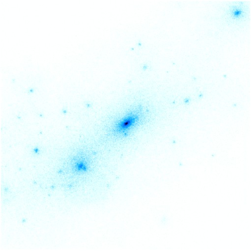
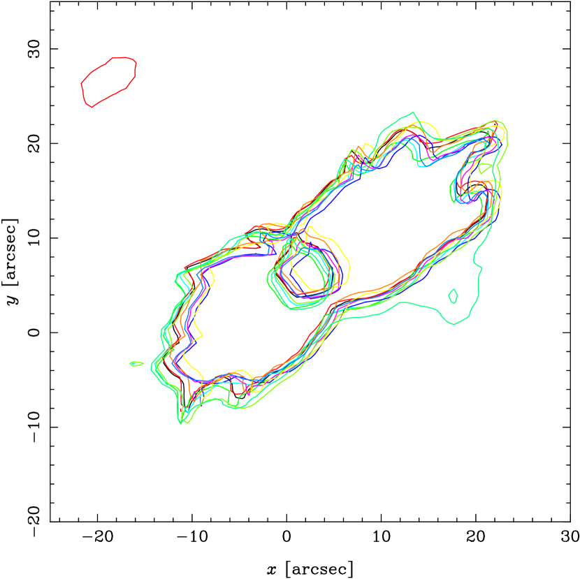
Figure 3.— (Left) A simulated cluster at $z=0.29$ used to generate arcs. The cluster has a virial mass of $M=10^{14.5}\,h^{-1}M_{\odot}$ and $c_{\rm vir}=7$. The side length is $2\,h^{-1}$ Mpc comoving. (Right) The $z_{\rm src}=5$ critical lines for this cluster. The black curve corresponds to the critical lines for no intervening lens planes, and the colored curves are the critical lines for 10 different realizations of the intervening matter.

In order to ensure that strong lensing occurs, we insert an extra lens plane containing a massive cluster, along with all the surrounding matter within $5h^{-1}$Mpc. An example of one of the clusters used is shown in fig. 3. We have used only clusters with regular, relaxed cores, since clusters with multiple massive components require more sophisticated modeling than is feasible using automated routines. We first generate arcs at multiple source planes using only the cluster lens, neglecting the other lens planes tiling the light cone. This amounts to assuming that matter is unclustered at redshifts different than the cluster redshift. We fit these arcs using the projected NFW model, holding fixed the cosmological parameters, to create a starting model from which subsequent fits are started. Next, we tile the lightcone by randomly selecting slices as described above, and recompute the ray-trace. We again generate sets of strongly lensed sources, and model the mock data sets using single-plane mass models, starting from the models which best fit the single-plane lens data, optimizing over both lens parameters and the cosmological parameters $\Omega_{M}$ and $w$. In general, the lensing properties of the clusters remain quite similar with and without the extra lens planes. For example, the right panel of fig. 3 shows the critical curves for the cluster shown in the left panel, for sources at $z_{\rm src}=5$, and it is apparent that the critical curves are only slightly affected by the LOS density fluctuations. Similarly, the total lensing cross sections and optical depth are negligibly affected by inclusion of the LOS material.

Figure 4.— Cosmological parameters derived from fitting sets of 50 strongly lensed sources between redshifts $z_{\rm src}=0.8$ to 5, generated by ray-tracing through N-body simulations with full lightcone tiling. Each point corresponds to a realization of the intervening planes and lensed images. An input cosmology of $\Omega_{M}=0.3$, $w=-1$ was used to generate the lensed images.

Nevertheless, considerable errors in the derived cosmological parameters can arise from projection noise as well as deviations of the cluster profiles from the simple NFW form. Figure 4 shows results from our ray-tracing simulations. As is apparent from the figure, quite large, biased errors can arise from the combination of effects discussed above. The 95% confidence regions for the two fitted parameters are $0.13<\Omega_{M}<0.45$ and $-3.3<w<-0.7$ with mean values of $\langle\Omega_{M}\rangle=0.3$ and $\langle w\rangle=-1.3$, for input values of $\Omega_{M}=0.3$ and $w=-1$.

4. Cleaning out the noise

The sources of noise discussed above pose serious challenges to the use of giant arcs for cosmography, however they are not necessarily insurmountable. Modeling uncertainties can be removed by observing large numbers of arcs in each cluster, so that a nonparametric, unbiased reconstruction of the mass profile and cosmology may be performed. This requires high resolution and deep imaging, along with redshifts for the arcs.

Projection noise appears more recalcitrant. Directly measuring the intervening mass fluctuations with weak lensing (e.g. Taylor, 2001) is difficult, in part because the main lens cluster must be carefully subtracted, but also because weak lensing can only measure the fluctuations on scales larger than a few arcminutes, while the strong lensing region is sensitive to power down to sub-arcminute scales (Dalal et al., 2003). Another possible means of cleaning out the projection noise would be to reconstruct the density and shear fluctuations along the line-of-sight using the observed galaxies in the field. This is not unreasonable, since we know that most of the power on the relevant $\sim$arcminute scales is produced by halos (Seljak, 2000). However, previous attempts at such reconstructions have not been entirely successful, with different groups finding quite different shear and convergence over the same field (e.g. Lewis & Ibata, 2001; Riess et al., 2001; Mörtsell et al., 2001; Benítez et al., 2002b).

The main difficulty with predicting the lensing convergence and shear fields from the field galaxies is that galaxies and mass are not perfectly correlated. Recall that we must be able to suppress the projection noise by at least 1-2 orders of magnitude in order to derive useful cosmological constraints from multiple arcs in a single cluster. Unfortunately, the cross-correlation between galaxies and mass, $r=P_{gm}/(P_{gg}P_{mm})^{1/2}$, is expected to be less than unity, typically of order $r\sim 0.5$ on the relevant scales. This would appear to preclude a sufficiently accurate reconstruction. Another way to understand this is as follows. Reconstructing the convergence and shear arising from individual galaxies in the field involves associating halos of mass $M$ with galaxies of luminosity $L$. Unfortunately, the relation between $M$ and $L$ is not one-to-one. For example, a galaxy like the Milky Way may be the central galaxy in halo of mass $10^{12}M_{\odot}$, or it may be a member of a group an order of magnitude larger in mass. In the halo occupation distribution model of Kravtsov et al. (2004), there is roughly a factor of $3-5$ uncertainty in the mass of a halo hosting a given galaxy, which directly translates into the uncertainty in the convergence and shear associated with the galaxy. Even if central galaxies may be distinguished from satellite galaxies, there is still an unknown scatter in the relation between halo mass and central galaxy luminosity (Tasitsiomi et al., 2004; Abazajian et al., 2004). In addition, halo triaxiality and substructure will affect the convergence and shear at the level of interest.

One crude test of the reconstruction method may be possible using extant cosmic shear data. Using the observed foreground galaxies in the field, one can make a prediction for the cosmic shear as a function of position, which can be checked against the values actually observed. This unfortunately cannot test the fidelity of the reconstruction on the required $\sim 10\arcsec$ scales, since shot noise in the source galaxies typically limits the resolution of shear maps to arcminute scales. While this cannot fully validate the method, a test along these lines would be a worthwhile indicator of whether significant observational efforts should be devoted towards the use of giant arcs to constrain geometry.

5. Summary

We have quantified various sources of noise expected in strong lensing cosmography. The use of multiple arcs in galaxy clusters holds great promise towards constraining the properties of dark energy, however significant errors can arise from line-of-sight projections and modeling uncertainties. Removing the projection noise to the necessary level appears difficult, since reconstruction of the mass density along the line of sight is hampered by the fact that mass and light are not perfectly correlated. If projection noise cannot be adequately cleaned out, then we cannot use “golden lenses”, but must instead average over many strong lensing clusters in order to derive useful cosmological constraints. To avoid biases in the inferred cosmological parameters, highly flexible or nonparametric mass models must be used to describe the cluster. In the absence of any knowledge of cluster density profiles, non-parametric models require large numbers of arcs to be observed in each cluster to sufficiently constrain the mass model. However, in principle one could use N-body simulations to impose prior constraints on cluster profiles. Using priors from N-body simulations would not be useful for individual systems, because of the large scatter in profiles among individual clusters. However, if simulated clusters do provide a reasonable description of the population of real galaxy clusters, then priors derived from simulations may allow useful cosmological constraints to be derived from large ensembles of lensing clusters. Meneghetti et al. (2004) make preliminary investigations into this approach. It may also be worthwhile to investigate whether additional information, such as X-ray temperature profiles of lensing clusters, can be used to improve the cosmological constraints derived from giant arcs.

Appendix A Covariance matrix

Consider a model for a lens system with $n_{\rm obs}$ observables ${\bm{O}}$ and $n_{p}$ parameters ${\bm{p}}$ describing the lens (and possibly cosmology as well). Assume that the penalty function may be written $\chi^{2}=\bm{\delta O}\cdot{\bf V}\cdot\bm{\delta O}$, where ${\bf V}^{-1}=\langle{\bm{\delta O\,\delta O}}\rangle$ describes the covariance of the observational errors. For each lensed source, there are additionally $m$ parameters, with $m=2$ if only the image positions are being modeled, or $m=3$ if the fluxes are modeled as well. The $m\,n_{\rm src}$ source parameters are nuisance parameters, over which we marginalize to obtain the $n_{p}\times n_{p}$ covariance matrix and its inverse, the Fisher matrix ${\bf F}$. If ${\bf D}=\partial{\bm{O}}/\partial{\bm{p}}$, then propagating errors we have ${\bf F}={\bf D}^{\sf T}\cdot{\bf V}\cdot{\bf D}$. For a single source, the (unmarginalized) Fisher matrix takes the form

$$\bordermatrix{n_{p}\mbox{\large\{}&\overbrace{\bf A}^{\displaystyle n_{p}}&\overbrace{\bf B}^{\displaystyle m}\cr m\,\mbox{\large\{}&{\bf B}^{\sf T}&{\bf C}\cr},$$ (A1)

where the $n_{p}\times n_{p}$ block ${\bf A}$ corresponds to the lens parameters, the $m\times m$ block ${\bf C}$ corresponds to the source parameters, and the $n_{p}\times m$ block ${\bf B}$ is the cross term. Marginalizing over the source parameters, the resulting Fisher matrix becomes ${\bf F}={\bf A}-{\bf B}\cdot{\bf C}^{-1}\cdot{\bf B}^{\sf T}$.

For multiple sources, the full (unmarginalized) Fisher matrix has the form

$${\bf F}_{u}=\left(\begin{array}[]{ccccc}\sum_{i}{\bf A}_{i}&{\bf B}_{1}&{\bf B}_{2}&{\bf B}_{3}&\ldots\\ {\bf B}_{1}^{\sf T}&{\bf C}_{1}&0&0&\ldots\\ {\bf B}_{2}^{\sf T}&0&{\bf C}_{2}&0&\\ {\bf B}_{3}^{\sf T}&0&0&{\bf C}_{3}&\\ \vdots&\vdots&&&\ddots\end{array}\right).$$ (A2)

Here, ${\bf A}_{i}$, ${\bf B}_{i}$, and ${\bf C}_{i}$ are the components of the single-source Fisher matrices (eqn. A1) for source $i$. We wish to invert ${\bf F}_{u}$ to obtain the parameter covariance matrix. We can do so by noting that ${\bf F}_{u}$ is diagonalized by the transformation

$${\bf U}\cdot{\bf F}_{u}\cdot{\bf U}^{\sf T}=\left(\begin{array}[]{cccc}{\bf F}_{\rm tot}&0&0&\ldots\\ 0&{\bf C}_{1}&0&\ldots\\ 0&0&{\bf C}_{2}&\\ \vdots&\vdots&&\ddots\end{array}\right),$$ (A3)

where

$${\bf U}=\left(\begin{array}[]{cc}\mathbbm{1}&\begin{array}[]{ccc}-{\bf B_{1}}{\bf C}_{1}^{-1}&-{\bf B_{2}}{\bf C}_{2}^{-1}&\ldots\end{array}\\ \begin{array}[]{c}0\\ 0\\ \vdots\end{array}&{\mbox{\Huge$\mathbbm{1}$}}\end{array}\right),$$ (A4)

and ${\bf F}_{\rm tot}=\sum_{i}{\bf F}_{i}=\sum_{i}{\bf A}_{i}-{\bf B}_{i}\cdot{\bf C}_{i}^{-1}\cdot{\bf B}_{i}^{\sf T}$. From this, it is easy to see that

$${\bf F}_{u}^{\,-1} = {\bf U}^{\sf T}\cdot\left(\begin{array}[]{cccc}{\bf F}_{\rm tot}^{\,-1}&0&0&\ldots\\ 0&{\bf C}_{1}^{-1}&0&\ldots\\ 0&0&{\bf C}_{2}^{-1}&\\ \vdots&\vdots&&\ddots\end{array}\right)\cdot{\bf U}$$ (A9)

$$= \left(\begin{array}[]{cccc}{\bf F}_{\rm tot}^{\,-1}&-{\bf F}_{\rm tot}^{-1}{\bf B}_{1}{\bf C}_{1}^{-1}&-{\bf F}_{\rm tot}^{-1}{\bf B}_{2}{\bf C}_{2}^{-1}&\ldots\\ -{\bf C}_{1}^{-1}{\bf B}_{1}^{\sf T}{\bf F}_{\rm tot}^{-1}&{\bf C}_{1}^{-1}+{\bf C}_{1}^{-1}{\bf B}_{1}^{\sf T}{\bf F}_{\rm tot}^{-1}{\bf B}_{1}{\bf C}_{1}^{-1}&{\bf C}_{1}^{-1}{\bf B}_{1}^{\sf T}{\bf F}_{\rm tot}^{-1}{\bf B}_{2}{\bf C}_{2}^{-1}&\ldots\\ -{\bf C}_{2}^{-1}{\bf B}_{2}^{\sf T}{\bf F}_{\rm tot}^{-1}&{\bf C}_{2}^{-1}{\bf B}_{2}^{\sf T}{\bf F}_{\rm tot}^{-1}{\bf B}_{1}{\bf C}_{1}^{-1}&{\bf C}_{2}^{-1}+{\bf C}_{2}^{-1}{\bf B}_{2}^{\sf T}{\bf F}_{\rm tot}^{-1}{\bf B}_{2}{\bf C}_{2}^{-1}&\\ \vdots&\vdots&&\ddots\end{array}\right)$$ (A14)

The covariance of the $n_{p}$ lens parameters is given by the upper left $n_{p}\times n_{p}$ block ${\bf F}_{\rm tot}^{\,-1}$. Therefore, the full (many-source) marginalized Fisher matrix is simply the sum of the marginalized single-source Fisher matrices, as we might have expected.

Appendix B Large-scale structure

Density fluctuations along the line of sight will perturb the lensed images, inducing changes in the derived best-fitting lens parameters. Dalal & Kochanek (2002) compute the perturbations to the parameters to first order in the density and shear perturbations, which is sufficient for our purposes (recall that the rms convergence fluctuations are $\langle\kappa^{2}\rangle^{1/2}\simeq 1\%$). The only minor modification here is that multi-plane lens factors must be included (Schneider et al., 1992; Keeton, 2003).

Let us parametrize the line-of-sight fluctuations by projecting the density and shear onto additional lens planes. Each plane has its own surface density perturbation $\delta\Sigma$ (measured relative to mean density) and (2-component) tidal shear $\delta\Gamma$, so that for $N$ additional planes we have $n_{q}=3N$ variables, which we denote by $n_{q}$ element $\bm{q}$. Just as shifts in the lens parameters $\Delta\bm{p}$ produce shifts in the observables $(\partial\bm{O}/\partial\bm{p})\Delta\bm{p}$, the line of sight fluctuations produce shifts $(\partial\bm{O}/\partial\bm{q})\Delta\bm{q}$. Minimizing $\chi^{2}$, this implies that the LOS fluctuations induce parameter shifts

$$\Delta\bm{p} = {\bf F}_{u}^{\,-1}\cdot\left(\frac{\partial\bm{O}}{\partial\bm{p}}\right)^{\sf T}\cdot{\bf V}\cdot\frac{\partial\bm{O}}{\partial\bm{q}}\cdot\Delta\bm{q}$$ (B1)

$$\equiv {\bf M}\cdot\Delta\bm{q}.$$

We are mainly interested in the induced shifts in the lens parameters and cosmological parameters, not the nuisance parameters describing the sources. Let us write the first $n_{p}$ elements of the full parameter array $\bm{p}$ as ${\bm{p}}_{\rm lens}$, and the $m$ nuisance parameters for each of the sources as $\bm{u}$. Using the above expression for ${\bf F}_{u}$ (eqn. A9), we can write the first $n_{p}$ rows of eqn. B1 as a sum over independent terms for each source,

$${\bf M}_{1\ldots n_{p}}={\bf F}_{\rm tot}^{\,-1}\sum_{i}^{n_{\rm src}}\left[\left(\frac{\partial\bm{O}_{i}}{\partial\bm{p}_{\rm lens}}\right)^{\sf T}-{\bf B}_{i}{\bf C}_{i}^{-1}\left(\frac{\partial\bm{O}}{\partial\bm{u}}\right)_{i}^{\sf T}\right]\cdot{\bf V}\cdot\frac{\partial\bm{O}_{i}}{\partial\bm{q}}.$$ (B2)

Given our expression for ${\bf M}$, the parameter covariance caused by LOS fluctuations is $\langle\Delta p_{i}\Delta p_{j}\rangle=M_{i\alpha}\langle\Delta q_{\alpha}\Delta q_{\beta}\rangle M_{j\beta}$.

References

- Abazajian et al. (2004) Abazajian, K., Zheng, Z., Zehavi, I., Weinberg, D. H., Frieman, J. A., Berlind, A. A., Blanton, M. R., Bahcall, N. A., Brinkmann, J., Schneider, D. P., & Tegmark, M. 2004, ArXiv Astrophysics e-prints, astro-ph/0408003
- Barkana (1998) Barkana, R. 1998, ApJ, 502, 531
- Benítez et al. (2002a) Benítez, N., Broadhurst, T. J., Ford, H., Blakeslee, J. P., Illingworth, G. D., Postman, M., Bouwens, R., Coe, D., Tran, H. D., Tsvetanov, Z. I., White, R. L., Zekser, K., & ACS, I. D. T. 2002a, Bulletin of the American Astronomical Society, 34, 1236
- Benítez et al. (2002b) Benítez, N., Riess, A., Nugent, P., Dickinson, M., Chornock, R., & Filippenko, A. V. 2002b, ApJ, 577, L1
- Bennett et al. (2003) Bennett, C. L., Halpern, M., Hinshaw, G., Jarosik, N., Kogut, A., Limon, M., Meyer, S. S., Page, L., Spergel, D. N., Tucker, G. S., Wollack, E., Wright, E. L., Barnes, C., Greason, M. R., Hill, R. S., Komatsu, E., Nolta, M. R., Odegard, N., Peiris, H. V., Verde, L., & Weiland, J. L. 2003, ApJS, 148, 1
- Blandford & Narayan (1992) Blandford, R. D. & Narayan, R. 1992, ARA&A, 30, 311
- Bode & Ostriker (2003) Bode, P. & Ostriker, J. P. 2003, ApJS, 145, 1
- Dalal et al. (2004) Dalal, N., Holder, G., & Hennawi, J. F. 2004, ApJ, 609, 50
- Dalal et al. (2003) Dalal, N., Holz, D. E., Chen, X., & Frieman, J. A. 2003, ApJ, 585, L11
- Dalal & Kochanek (2002) Dalal, N. & Kochanek, C. S. 2002, ApJ, 572, 25
- Ebeling et al. (2001) Ebeling, H., Edge, A. C., & Henry, J. P. 2001, ApJ, 553, 668
- Eisenstein & Hu (1999) Eisenstein, D. J. & Hu, W. 1999, ApJ, 511, 5
- Golse et al. (2002) Golse, G., Kneib, J.-P., & Soucail, G. 2002, A&A, 387, 788
- Gonzalez et al. (2002) Gonzalez, A. H., Zaritsky, D., Simard, L., Clowe, D., & White, S. D. M. 2002, ApJ, 579, 577
- Hennawi et al. (2004) Hennawi et al. 2004, in preparation
- Hoekstra et al. (2001) Hoekstra, H., Yee, H. K. C., & Gladders, M. D. 2001, ApJ, 558, L11
- Hu (2002) Hu, W. 2002, Phys. Rev. D, 66, 083515
- Hu & Jain (2003) Hu, W. & Jain, B. 2003, ArXiv Astrophysics e-prints, astro-ph/0312395
- Jain & Taylor (2003) Jain, B. & Taylor, A. 2003, Physical Review Letters, 91, 141302
- Keeton (2003) Keeton, C. R. 2003, ApJ, 584, 664
- Kochanek (2002) Kochanek, C. S. 2002, ApJ, 578, 25
- Kravtsov et al. (2004) Kravtsov, A. V., Berlind, A. A., Wechsler, R. H., Klypin, A. A., Gottloeber, S., Allgood, B., & Primack, J. R. 2004, ApJ, 609, 35
- Lewis & Ibata (2001) Lewis, G. F. & Ibata, R. A. 2001, MNRAS, 324, L25
- Limber (1954) Limber, D. N. 1954, ApJ, 119, 655
- Meneghetti et al. (2004) Meneghetti, M., Jain, B., Bartelmann, M., & Dolag, K. 2004, astro-ph/0409030
- Mörtsell et al. (2001) Mörtsell, E., Gunnarsson, C., & Goobar, A. 2001, ApJ, 561, 106
- Navarro et al. (1997) Navarro, J. F., Frenk, C. S., & White, S. D. M. 1997, ApJ, 490, 493
- Peacock & Dodds (1996) Peacock, J. A. & Dodds, S. J. 1996, MNRAS, 280, L19
- Riess et al. (2001) Riess, A. G., Nugent, P. E., Gilliland, R. L., Schmidt, B. P., Tonry, J., Dickinson, M., Thompson, R. I., Budavári, T., Casertano, S., Evans, A. S., Filippenko, A. V., Livio, M., Sanders, D. B., Shapley, A. E., Spinrad, H., Steidel, C. C., Stern, D., Surace, J., & Veilleux, S. 2001, ApJ, 560, 49
- Riess et al. (2004) Riess, A. G., Strolger, L., Tonry, J., Casertano, S., Ferguson, H. C., Mobasher, B., Challis, P., Filippenko, A. V., Jha, S., Li, W., Chornock, R., Kirshner, R. P., Leibundgut, B., Dickinson, M., Livio, M., Giavalisco, M., Steidel, C. C., Benitez, N., & Tsvetanov, Z. 2004, ApJ, 607, 665
- Schneider et al. (1992) Schneider, P., Ehlers, J., & Falco, E. E. 1992, Gravitational Lenses (Gravitational Lenses, XIV, 560 pp. 112 figs.. Springer-Verlag Berlin Heidelberg New York. Also Astronomy and Astrophysics Library)
- Seljak (2000) Seljak, U. 2000, MNRAS, 318, 203
- Seljak et al. (2004) Seljak, U., Makarov, A., Mandelbaum, R., Hirata, C. M., Padmanabhan, N., McDonald, P., Blanton, M. R., Tegmark, M., Bahcall, N. A., & Brinkmann, J. 2004, submitted to PRD, astro-ph/0406594
- Sheldon et al. (2004) Sheldon, E. S., Johnston, D. E., Frieman, J. A., Scranton, R., McKay, T. A., Connolly, A. J., Budavári, T., Zehavi, I., Bahcall, N. A., Brinkmann, J., & Fukugita, M. 2004, AJ, 127, 2544
- Soucail et al. (2004) Soucail, G., Kneib, J.-P., & Golse, G. 2004, accepted to A&A, astro-ph/0402658
- Tasitsiomi et al. (2004) Tasitsiomi, A., Kravtsov, A. V., Wechsler, R. H., & Primack, J. R. 2004, submitted to ApJ, astro-ph/0404168
- Taylor (2001) Taylor, A. N. 2001, astro-ph/0111605
- Wambsganss et al. (2003) Wambsganss, J., Bode, P., & Ostriker, J. P. 2003, ApJ, 606, L93
- Zhang et al. (2003) Zhang, J., Hui, L., & Stebbins, A. 2003, submitted to ApJ, astro-ph/0312348