WMAP Microwave Emission Interpreted as Dark Matter Annihilation in the Inner Galaxy

Abstract

Excess microwave emission observed in the inner Galaxy (inner $\sim 1-2$ kpc) is consistent with synchrotron emission from highly relativistic $e^{+}e^{-}$ pairs produced by dark matter particle annihilation. More conventional sources for this emission, such as free-free (thermal bremsstrahlung), thermal dust, spinning dust, and the softer Galactic synchrotron traced by low-frequency surveys, have been ruled out. The total power observed in the range $23<\nu<61{\rm~{}GHz}$ is between $1\times 10^{36}$ and $5\times 10^{36}{\rm~{}erg}{\rm~{}s}^{-1}$, depending on the method of extrapolation to the Galactic center, where bright foreground emission obscures the signal. The inferred electron energy distribution is diffusion hardened, and is in qualitative agreement with the energy distribution required to explain the gamma ray excess in the inner Galaxy at $1-30{\rm~{}GeV}$ as inverse-Compton scattered starlight. We investigate the possibility that this population of electrons is produced by dark matter annihilation of $100{\rm~{}GeV}$ particles, with cross section $\langle\sigma_{A}v\rangle=2\times 10^{-26}{\rm~{}cm}^{3}{\rm~{}s}^{-1}$, and an $r^{-1}$ dark matter mass profile truncated in the inner Galaxy, and find this scenario to be consistent with current data.

1 INTRODUCTION

It is almost universally accepted that the majority of matter in the Universe is non-baryonic. Existence of this “dark matter” is supported by several kinds of evidence: galaxy rotation curves, gravitational lensing of background objects by galaxy clusters, the small value of $\Omega_{b}h^{2}$ determined from big bang nucleosynthesis, and $\Omega_{b}/\Omega_{m}$ from the cosmic microwave background (CMB) anisotropy. The gravitational effects of dark matter are observed, but in spite of numerous investigations with particle accelerators and direct detection experiments, no direct signature of dark matter interaction with ordinary matter has ever been found.

Supersymmetry theory (SUSY) provides a candidate dark matter particle: a linear combination of higgsino, Z-ino, and photino states commonly known as the neutralino, $\chi$, the lightest stable supersymmetric particle (See Jungman, Kamionkowski, & Griest 1996 for a review). Direct detection of neutralinos is difficult because of their very weak interactions with ordinary matter, but if the neutralino is a Majorana fermion (and therefore is its own anti-particle, $\chi=\bar{\chi}$), it self-annihilates and produces some combination of W and Z bosons, mesons, $e^{+}e^{-}$ pairs, and $\gamma$-rays (see Gunn et al.  1978 for the basic scenario). Baltz & Wai (2004) point out that a significant fraction of the power liberated in self-annihilation may go into ultra-relativistic $e^{+}e^{-}$ pairs (hereafter “electrons”), producing observable microwave synchrotron radiation. These high energy electrons inverse Compton scatter CMB and starlight photons, shifting them to soft and hard $\gamma$-rays, respectively. To date, efforts have focused largely on $\gamma$-ray observations of dark matter concentrations in dwarf spheroidal galaxies (Gondolo 1994, Blasi et al.  2003, Baltz & Wai 2004) or the Galactic center (Stoehr et al.  2003), or synchrotron observations of satellite galaxies (Baltz & Wai 2004). Direct detection of high energy positrons near Earth has also been discussed (Baltz & Edsjö 1998, Baltz et al.  2002), but is thought to be unlikely, given the foreground produced by other mechanisms and the high boost factors required to obtain an observable signal (Hooper et al.  2004). Copious annihilation near the black hole in the Galactic center would be detectable at radio frequencies for most neutralino models if there were a steep central cusp in the density profile (Gondolo 2000) but non-detection may indicate lack of a cusp. Detection of synchrotron emission near the black hole in the Galactic center has also been considered (Bertone et al.  2002, Aloisio et al.  2004) but detection of the synchrotron annihilation signal in the inner regions ($\sim 1$ kpc) of the Galaxy was thought to be impractical because of the complexity of the ISM microwave emission from other components (thermal dust, spinning dust, free-free, and “ordinary” synchrotron from shock-accelerated electrons). Recent advances in our understanding of ISM emission have made this problem tractable.

The Wilkinson Microwave Anisotropy Probe (WMAP) has revealed the structure of the Galactic ISM with unprecedented precision at microwave ($22-94{\rm~{}GHz}$) frequencies, leading to a reassessment of the Galactic foregrounds (Bennett et al.  2004, Finkbeiner 2004, Finkbeiner et al.  2004). One surprising result of the increasingly careful foreground analysis is an excess of emission in the inner Galaxy, distributed with (approximate) radial symmetry within $\sim 20^{\circ}$ of the Galactic center (dubbed the “haze,” Finkbeiner 2004). This emission is not correlated with any of the foreground templates representing the known microwave foregrounds. Although the spectrum of this excess is somewhat flatter than standard synchrotron emission, we argue that it is consistent with a population of ultra-relativistic electrons created in the inner Galaxy and diffusing outward, and consider the possibility that these electrons are products of dark matter (DM) annihilation. To be concrete, we refer to the DM particle as the neutralino throughout, although any stable neutral particle with a mass of $\sim 100{\rm~{}GeV}$ and the assumed $\langle\sigma_{A}v\rangle$ would have the consequences described below.

Assuming the neutralino is the dominant form of dark matter, the average relic density today is $\Omega_{\chi}h^{2}=(\Omega_{m}-\Omega_{b})h^{2}=0.113\pm.009$ according to the WMAP cosmology (Spergel et al.  2003). By setting the annihilation rate equal to the expansion rate after freeze-out, the cross section $\langle\sigma_{A}v\rangle$ is determined by this relic abundance (see §3.1). Using a fiducial mass of $100{\rm~{}GeV}$, a diffusion term ($K$) derived from cosmic ray data, and an energy loss term ($AE^{2}$) including synchrotron losses and inverse Compton scattering (ICS) off of starlight and CMB photons, we calculate the electron energy distribution as a function of Galactocentric radius for various assumptions. An analytic solution is presented for the simplest case, and numerical solutions for variable $A$ and $K$ terms.

For the assumed dark matter distribution, all models produce a similar (factor of $\sim 2$) power output, since the power input by annihilation is fixed a priori. In all cases, the spectrum, morphology, and predicted synchrotron power output by the model is similar to the observed WMAP excess. This is tantalizing, because if one can determine the losses (i.e. energy density of starlight and magnetic field) in the inner Galaxy, the fraction of power liberated as relativistic $e^{+}e^{-}$, and the dark matter density profile, then the total $\chi$ annihilation power can be computed. Given the dark matter distribution and the annihilation power in the inner Galaxy, the approximate mass, $m\chi$, can be computed. With luck, an annihilation line or sharp cut off in $\gamma$ ray continuum will be observed, fixing the mass more precisely. With refined Galactic models and improved microwave and $\gamma$ ray data, it may actually be possible to determine the mass and cross section of a new particle astrophysically, making a specific prediction to be verified by accelerator experiments (e.g. at the LHC, Ellis et al.  2004).

The main difference between our model and previous models is that electron diffusion is solved for in a self-consistent way (like Baltz & Wai 2004) and its effect on the synchrotron spectrum computed. The consequent flattening of the spectrum, especially near the Galactic Center, has not been emphasized in the previous literature.

In §2, the excess microwave emission near the Galactic Center is described. Model parameters for the hot electron population and ISM are justified in §3, and the model is evaluated and compared to WMAP data in §4.

2 THE WMAP HAZE

The Wilkinson Microwave Anisotropy Probe (WMAP) has observed the sky with good sensitivity ($\sim 150\mu{\rm K}$ per pixel in the 1 yr data) and measured the cosmological anisotropy power spectrum (Hinshaw et al.  2003) and, with less significance, its polarization (Page et al.  2003), in order to determine fundamental cosmological parameters (Spergel et al.  2003). To the extent that Galactic foreground signals from thermal dust emission, free-free (thermal bremsstrahlung), “ordinary” synchrotron (relativistic electrons accelerated by supernovae and spiraling in the Galactic magnetic field) and spinning dust (see Draine & Lazarian 1998) are present in the data, they have been removed and do not interfere with the cosmological signal (Bennett et al.  2003).

In the course of studying these foregrounds and exploring the possibility of spinning dust (Finkbeiner 2004, Finkbeiner et al.  2004), evidence for an additional emission component has emerged. This enigmatic emission is centered at the Galactic center and extends $20-30^{\circ}$ away in all directions, falling rapidly ($\sim 1/R$) with projected distance from the Galactic center. It is not likely to be an artifact of the foreground subtraction, because south of the GC it is similar in brightness to the other components, and the fit is sufficiently rigid (only eight parameters for the whole sky to fit 5 bands $\times 3\times 10^{6}$ pixels) that it is robust to errors in the templates. Even north of the GC, the excess is approximately symmetrical about the GC in spite of much brighter foreground objects such as the large ($\sim 10^{\circ}$) nearby nebula of $\zeta$Oph. This emission component has been nicknamed “the haze” to avoid giving it an interpretive name prematurely (see Finkbeiner 2004).

The haze was first thought to be a free-free component from gas too hot to have recombination line emission ($T>>10^{4}{\rm~{}K}$) and too cold to have significant X-ray emission in the ROSAT (Snowden et al.  1997) 1.5 keV band ($T<<10^{6}{\rm~{}K}$). North of the GC there is sufficient gas and dust to hide the H$\alpha$ recombination line and X-ray emission, but to the South, column densities are low enough that both would be seen. For $\sim 10^{5}{\rm~{}K}$ gas the X-ray emission would be soft enough that gas absorption could block it, but gas is thermally unstable at $10^{5}$ K because of efficient metal-line cooling (e.g., Spitzer 1978), and the amount of gas required is inconsistent with H II column densities determined from pulsar dispersion measures given by Taylor & Cordes (1993). Furthermore, the free-free spectrum of $10^{5}$ K H II extends up to $\nu\sim 10^{7}{\rm~{}GHz}$ and the integrated spectral power suggests a substantial free-free power output of $1-5\times 10^{40}{\rm~{}erg}\sec^{-1}$. It is necessary to consider alternative sources of emission.

3 PARAMETERS

In this section, the model parameters are specified: annihilation cross section, mass, $e^{+}e^{-}$ energy distribution, magnetic field strength, photon field available for ICS, and dark matter mass profile in the Milky Way. The parameters are listed in Table 1.

3.1 Neutralino Cross Section

If the neutralinos present today are the cosmological relic of thermal production in the early Universe, then the mean neutralino mass density as a fraction of the critical density, $\Omega_{\chi}$ can be computed from its mass and cross section. The WMAP cosmology (Spergel et al.  2003) gives $\Omega_{DM}h^{2}=(\Omega_{m}-\Omega_{b})h^{2}=0.113\pm.009$, where the subscripts “DM”, “m” and “b” denote “dark matter”, “total matter” and “baryon”, respectively, and $h$ is the Hubble constant in units of $100{\rm~{}km}{\rm~{}s}^{-1}{\rm~{}Mpc}^{-1}$.

The neutralino number density falls rapidly when the temperature of the Universe ($T$) falls much below the particle mass ($m_{\chi}$). After this, neutralino annihilations cause the number density, $n$, to drop rapidly [$n\sim\exp(-m_{\chi}c^{2}/kT)$] to the level where the particle annihilation rate ($\Gamma$) is comparable to the expansion rate, $H(t)\sim\dot{a}/a\sim t^{-1}$, after which the comoving density asymptotes to the “freeze-out” density. In the early, radiation-dominated, Universe, $t\sim a^{2}$, so the criterion is

$$\Gamma=\langle\sigma_{A}v\rangle n\sim\langle\sigma_{A}v\rangle n_{0}a^{-3}\sim H\sim a^{-2}$$ (1)

where $n_{0}=na^{3}$ is the co-moving number density. Because temperature $T\sim a^{-1}$,

$$n_{0}T_{f}\sim\frac{1}{\langle\sigma_{A}v\rangle}$$ (2)

where $T_{f}\sim m_{\chi}$ is the freeze-out temperature, proportional to the particle mass. This leads to the remarkable conclusion that the co-moving relic mass density, $\rho_{\chi}=n_{0}m_{\chi}$, is inversely proportional to the cross section, so if one knows the relic mass density today (or assumes it) the cross section is fixed. A more complete calculation (Jungman et al.  1996) yields the same relation in terms of $\rho_{\chi}\sim\Omega_{\chi}h^{2}$:

$$\Omega_{\chi}h^{2}=\frac{3\times 10^{-27}{\rm~{}cm}^{3}{\rm~{}s}^{-1}}{\langle\sigma_{A}v\rangle}$$ (3)

A proper calculation of the relic density takes account of the form of the density drop after freeze-out and introduces a weak mass dependence in the relic density, but the approximation given in Eq. (3) is adequate for our purposes, and we adopt $\langle\sigma_{A}v\rangle=2\times 10^{-26}{\rm~{}cm}^{3}{\rm~{}s}^{-1}$.

3.2 Neutralino Mass

We take the neutralino mass, $m_{\chi}$ to be $100{\rm~{}GeV}$, approximately at the weak scale, and lower than the bounds of $m_{\chi}<600{\rm~{}GeV}$ given by Ellis et al.  (2000), or $m_{\chi}<$ several TeV (Baltz & Gondolow 2004). This choice of mass is arbitrary, and is degenerate with the fraction of power going into energetic $e^{+}e^{-}$ given in §4.3.

3.3 Energy Distribution

There is considerable uncertainty in both the injection energy distribution and the effects of diffusion on the resultant number density per energy, $n(E,r)$. One possible assumption is that annihilating neutralinos go directly to quark anti-quark pairs which then go to pions:

$$\chi\bar{\chi}\rightarrow\gamma+\pi^{o},\pi^{+},\pi^{-}$$

The pions then decay:

$$\pi^{+}\rightarrow\mu^{+}+\nu_{\mu}$$

$$\pi^{-}\rightarrow\mu^{-}+\bar{\nu}_{\mu}$$

followed by

$$\mu^{+}\rightarrow e^{+}+\nu_{e}+\bar{\nu}_{\mu}$$

$$\mu^{-}\rightarrow e^{-}+\bar{\nu}_{e}+\nu_{\mu}$$

This results in an injection energy distribution that goes as $n_{i}\sim E^{-3/2}$ in the low energy limit (see Blasi et al.  2003), with a significant fraction of the energy carried away by neutrinos. However, if annihilation to $\tau$ leptons is important ($\chi\bar{\chi}\rightarrow\tau^{+}\tau^{-}$) the resulting $e^{+}e^{-}$ spectrum would be harder (Hooper et al.  2004).

The injection spectrum must then be evolved through the diffusion and energy loss equations to determine the steady state electron density. The model in §4 assumes spherical symmetry, but one might also consider cylindrical symmetry with boundaries a few kpc from the Galactic midplane at which the electrons escape. If the electrons have time to diffuse to the boundaries before losing most of their energy, the electron spectrum can be considerably hardened. In the limit of rapid escape, the steady state spectrum is just the injection spectrum, so that sets a limit on the spectral hardness.

3.4 Photon energy density

The starlight photon energy density in the inner Galaxy is necessary to compute electron energy loss due to inverse Compton scattering. Strong et al. (2000) have considered a model based on IRAS and DIRBE infra-red data in addition to the usual stellar information, and find that the starlight energy density is approximately

$$U_{*}=11e^{-r/3{\rm~{}kpc}}{\rm~{}eV}{\rm~{}cm}^{-3}$$

in the Galactic plane, or about $0.6{\rm~{}eV}{\rm~{}cm}^{-3}$ at $r_{\sun}$. This compares to the energy density of $0.6{\rm~{}eV}{\rm~{}cm}^{-3}$ for a $\bar{B}=5\mu$G magnetic field, and $0.260\pm 0.001{\rm~{}eV}{\rm~{}cm}^{-3}$ for the CMB. The far IR emission is subdominant, but should be included in future models.

3.5 The Galactic Magnetic Field

Heiles (1996) presents measurements of different moments of the Galactic magnetic field in the plane at Galacto-centric distances of 4 and 8.5 kpc. None of these measurements is exactly the quantity we need, $\bar{B}=\langle B^{2}\rangle^{-1/2}$, but they are consistent with $\bar{B}=5\mu$G at the Solar circle and increasing exponentially toward the Galactic center. To demonstrate that our result is not strongly field dependent, we try two cases: $\bar{B}=5\mu$G, and $\bar{B}=21e^{-r/6{\rm~{}kpc}}\mu$G. This field is similar to the field radial dependence derived by Han (priv. comm.) with a scale length of $7.5{\rm~{}kpc}$. Because the $B$ field and starlight are so close to equipartition, we assume that they are exactly in equipartition for simplicity, even though there is no obvious mechanism to regulate this. Also, the field is assumed to be tangled in an isotropic way, so that the particles move in a random walk.

A more detailed model would incorporate what is known about field strength variation with position in the Galaxy, especially the fact that the field is stronger in the spiral arms than in inter-arm regions. Synchrotron emission is enhanced perpendicular to the field lines and suppressed along them; we assume isotropic tangling of the field and therefore isotropic emission. Furthermore, the ratio of the tangled to ordered strength, and the mean direction of the ordered part may be important. For example, Han (2004) suggests that the bulge is dominated by a solenoidal component perpendicular to the Galactic plane, which may facilitate rapid escape of electrons from the Galactic center, whereas particles created in the arms may be trapped there for longer periods of time. Therefore we should be cautious about applying conclusions drawn from local cosmic ray propagation to particles in the inner Galaxy. This is a rich subject, and is well beyond the scope of this article.

3.6 Mass profile

We assume a truncated Navarro, Frenk, & White (1997; NFW) profile. Because we are only interested in the inner $1-2{\rm~{}kpc}$ of the Galaxy, the larger scale shape of the NFW profile is unimportant to this calculation, other than that it serves to tie the assumed Milky Way mass (within 400 kpc) of $2\times 10^{12}M_{\sun}$ to a mass density at the center. We assume an NFW profile with $r_{s}=20$ kpc, and arbitrarily truncate the core at 600 pc. Although recent computer simulations indicate that NFW is not valid at the core Stoehr et al. (2003), there is theoretical support from the Jeans equation for an index of -1 or steeper in the core (Hansen 2004). In the case of a Moore (1998) profile ($\rho\sim r^{-1.4}$) the annihilation power can be a factor of 5 times higher. The details of the central truncation are unimportant for NFW profile (where each concentric shell contributes equal annihilation power) but becomes important for the Moore profile.

4 THE MODEL

4.1 Analytic Solution

At energies of tens of GeV, electrons moving in $\mu$Gauss fields take millions of years to lose half their energy, so it is a poor approximation to neglect electron diffusion. We assume that electrons resulting from the annihilation are created at a rate proportional to $\chi$ number density squared and then diffuse in a random walk through the (rather tangled) Galactic magnetic field. The number density $n(E,{\bf x})dE$ between energy $E$ and $E+dE$ evolves according to

$$\frac{d}{dt}n(E,{\bf x})=\nabla\cdot(K(E,{\bf x})\nabla n)+\frac{\partial}{\partial E}\left[b(E,{\bf x})n\right]+Q(E,{\bf x})$$ (4)

where $K(E,{\bf x})$ is the diffusion coefficient (area per time), $b(E,{\bf x})$ is the energy loss coefficient (energy loss per time), and $Q(E,{\bf x})$ is the source term (number density per time). Neglecting the position dependence of $K$ and $b$, the steady state equation is:

$$-K(E)\nabla^{2}n-\frac{\partial}{\partial E}\left[b(E)n\right]=Q(E,{\bf x}).$$ (5)

In the simple case where $K$ is energy independent and $b=-AE^{2}$ with $A$ constant, the solution for a mono-energetic delta-function source at the origin, $Q(E,{\bf x})\sim\delta({\bf x})\delta(E-E_{0})$, and zero density at $r=\infty$, is simply a superposition of spherically symmetric Gaussians losing energy and expanding with $\sigma^{2}\sim t$. The number density of electrons produced between $t$ and $t+dt$ in the past is

$$n(E(t),r)dE/dt=Q_{0}\frac{1}{[2\pi\sigma(t)^{2}]^{3/2}}\exp(-r^{2}/2\sigma(t)^{2})$$ (6)

with $Q_{0}$ the creation rate (number per second), and where electrons created with energy $E_{0}$ at $t=0$ lose energy as

$$b(t)=\frac{dE}{dt}=-AE^{2}$$ (7)

so that

$$E=\frac{E_{0}}{(1+AE_{0}t)}.$$ (8)

In general, the energy loss rate of each electron is

$$b=\frac{4}{3}\sigma_{T}c\gamma^{2}\beta^{2}(U_{B}+U_{\rm ph})$$ (9)

where $\sigma_{T}$ is the Thomson cross section, $\beta=v/c$ is the speed of the electron, $\gamma mc^{2}$ is the electron energy, $U_{B}=B^{2}/8\pi$ is the magnetic field energy density and $U_{\rm ph}$ is the photon energy density. In the ultra-relativistic limit,

$$A=\frac{4\sigma_{T}(U_{B}+U_{\rm ph})}{3m^{2}c^{3}},$$ (10)

where $U_{\rm ph}=U_{\rm star}+U_{\rm CMB}$. For electrons created time $t$ ago,

$$\sigma^{2}=2kt=\frac{2k(E_{0}-E)}{AE_{0}E}$$ (11)

so that the number density as an explicit function of energy is:

$$n(E,r)=Q_{0}\left[\frac{AE_{0}E}{4\pi k(E_{0}-E)}\right]^{3/2}\frac{1}{AE^{2}}\exp\left(\frac{-AE_{0}Er^{2}}{2k(E_{0}-E)}\right)$$ (12)

and the integral along the line of sight is

$$N(E,R)=\frac{Q_{0}E_{0}}{4\pi kE(E_{0}-E)}\exp\left(\frac{-AE_{0}ER^{2}}{2k(E_{0}-E)}\right)$$ (13)

where $R$ is the projected Galacto-centric distance. This Green function solution must be convolved with the projected source density to obtain the solution for arbitrary $Q$, but just this simple expression provides some intuition. (See Appendix A for more details). The energy distribution of the entire $e^{-}$ population is $n(E)\sim E^{-2}$, as one would obtain for a population created at energy $E_{0}$ and confined to a box. However, along any line of sight, the distribution is flatter ($\sim E^{-1}$) because of diffusion. The older electrons that have lost much of their energy have also had time to diffuse away from the source, leaving a flatter spectrum below some cut-off energy and a sharp drop above it. This cut-off energy decreases with distance from the source. Another feature of the above solution is that the total projected radial density $N(R)=\int dE~{}n(E,R)\sim r^{-1}$ diverges in the absence of a lower energy bound. This makes sense, because electrons have been created at rate $Q_{0}$ forever and never disappear. In reality, the diffusion zone in the Galaxy has finite size, and most electrons escape while still relativistic. The effects of this escape will be seen in the numerical solutions in the next section.

4.2 Numerical Solutions

For less restrictive assumptions about $K$, $A$, and $Q$, analytic solutions to Eq (4) are cumbersome or non-existent, and the PDE must be solved numerically. Being interested in the inner Galaxy, where dark matter density is assumed to be highest, we assume spherical symmetry and use the fact that the Laplacian of a radial function can be written

$$\nabla^{2}n(r)=\frac{1}{r}\frac{\partial^{2}}{\partial r^{2}}(rn).$$

It is convenient to solve for $rn(E,r)$ on a radius-energy $(r,E)$ grid and divide the result by $r$. In most cases a grid with 30 logarithmic energy bins $(0.1<E<100{\rm~{}GeV})$ and 60 radial bins $(0<r<r_{\rm max}=12000{\rm~{}pc})$ works well. Boundary conditions for $rn$ are taken to be zero at $r=0$ (as required) and $r=r_{\rm max}$ and an NFW profile squared as the input source distribution at maximum energy. The density is truncated in the inner 600 pc to the value at 600 pc to avoid the central cusp. Results are not sensitive to this truncation.

The matrix ${\bf M}$ describing the evolution of the system in state $S$ (i.e. $r$ times density at discretely sampled positions and energies) from time step $i$ to $i+1$ is constructed such that

$$S_{i+1}=S_{i}+{\bf M}S_{i}.$$

The steady state solution is the nullspace of ${\bf M}$ (i.e. ${\bf M}S=0$), readily found with SVD (singular-value decomposition). This is in general a multi-dimensional space providing exactly enough freedom to fit the boundary conditions stated above.

Grid solutions have been computed for two cases (in each case, $K_{0}=3\times 10^{-27}{\rm~{}cm}^{2}{\rm~{}s}^{-1}$ and $A_{0}=10^{-16}{\rm~{}s}^{-1}{\rm~{}GeV}^{-1}$): (1) $K=3K_{0},A=A_{0}$, and (2) $K(E)=3K_{0}(3^{\alpha}+(E/1{\rm~{}GeV})^{\alpha}$), $\alpha=0.6$, and $A$ representing the energy loss from synchrotron and scattering of CMB and starlight photons assuming equipartition of starlight and the magnetic field, and an exponential radial dependence (see Eq. 10).

The energy dependence of $K(E)$ given here is proportional to but somewhat higher than that found in the study of cosmic ray propagation in the Galaxy, including diffusion and convection, by Webber, Lee, & Gupta (1992). Although this study considered cosmic-ray nuclei and not leptons, at the high particle rigidity (momentum per charge) of interest, $e^{+}e^{-}$ diffuse in a similar fashion.

Figure 1: (top) Model 1 electron energy distribution for all electrons (thick line) and spherical shells of thickness $\Delta r=200{\rm~{}pc}$ at radii of 8, 4, 2, 1, and 0.4 kpc (thin lines, top to bottom) from the numerical calculation in §4.2. For comparison, the analytic solution in §4.1 is evaluated for all electrons (dashed line) and shells at the same radii (crosses). The numerical solution is a good approximation to the analytic solution at $E>1{\rm~{}GeV}$ and inner radii, where the WMAP emission is evaluated. (bottom) Number density (${\rm~{}pc}^{-3}$) as a function of Galacto-centric radius for all electrons (thick line) and for logarithmically spaced bins of energy 0.35, 1.1, 3.5, 11, 35, and 89 GeV (thin lines, top to bottom). The highest energy bin is truncated at 600 pc. In both panels the figures are normalized assuming a total annihilation rate of $4\times 10^{38}{\rm~{}s}^{-1}$ as found in Appendix A.

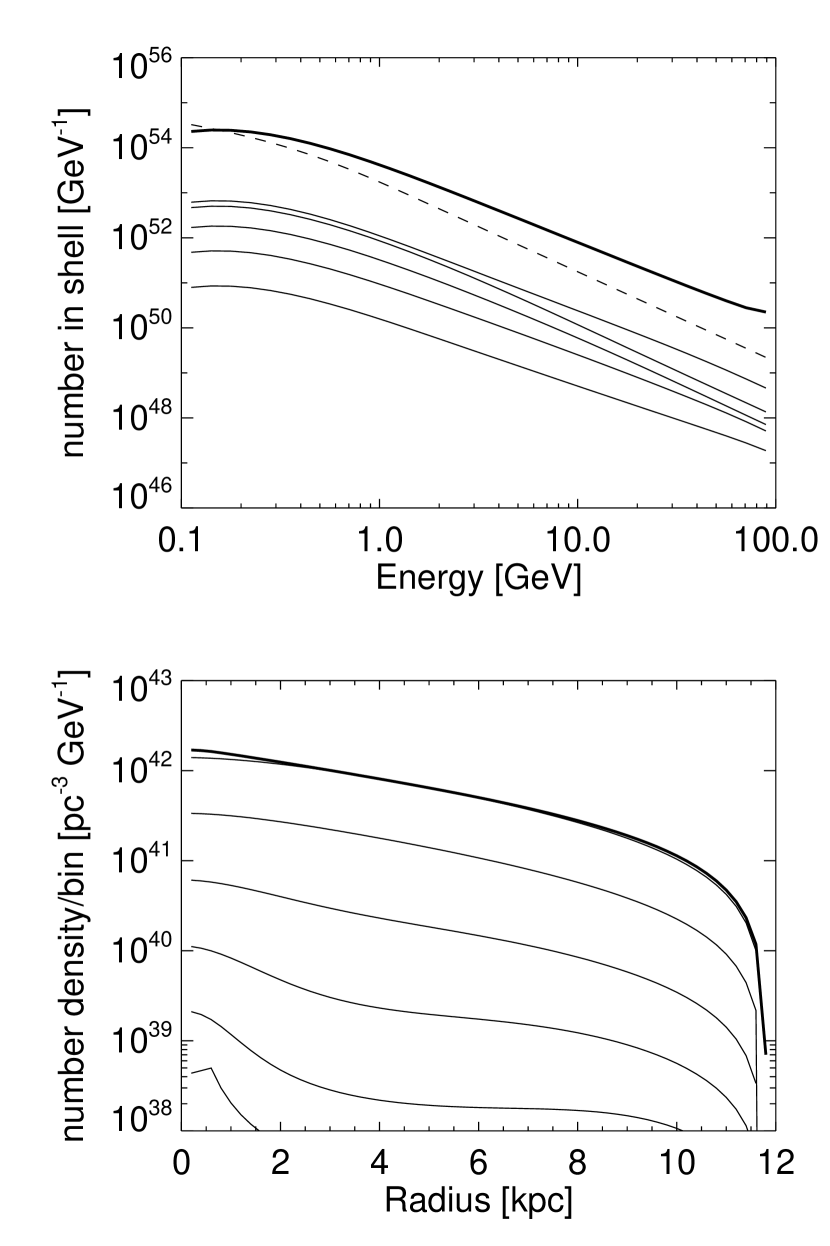
Figure 2: (top) Model 2 electron energy distribution for all electrons (thick line) and spherical shells as in Fig. 1 from the numerical calculation in §4.2. For comparison, the analytic solution for Model 1 is evaluated for all electrons (dashed line) as before. The slopes are somewhat steeper at high energy, but could be made flatter by changing the assumptions about the boundaries of the diffusion zone. (bottom) Number density (${\rm~{}pc}^{-3}$) as a function of Galacto-centric radius for all electrons (thick line) and for bins of energy 0.35, 1.1, 3.5, 11, 35, and 89 GeV (thin lines, top to bottom). The highest energy bin is truncated at 600 pc. In both panels the figures are normalized assuming a total annihilation rate of $4\times 10^{38}{\rm~{}s}^{-1}$.

Figure 3: (a) Line of sight electron energy distribution [${\rm~{}cm}^{-2}{\rm~{}GeV}^{-1}$]. Curves are shown for Galacto-centric angle $\theta=(2,5,10,20,$ and $50^{\circ})$. The numerical solution rolls off at lower energy because of electron escape from the diffusion zone. (b) Specific Intensity vs. frequency for lines of sight at the same angles. The spectra nearest the Galactic center are flattest, as discussed in §4.1. (c) Specific Intensity vs. $\theta$ for frequency bins centered at 23.8, 30.0, 37.8, 59.9, and 94.9 GHz, close to the WMAP frequencies, (highest to lowest). These calculations assume a total annihilation rate of $4\times 10^{38}{\rm~{}s}^{-1}$, and that all power goes into $e^{+}e^{-}$. These plots must be rescaled by a factor of 0.25 to obtain the model shown in Figure 4.

4.3 Electron Energy Distribution

The electron energy distribution for constant $A$ and $K$ (model 1) is shown in Figure 1, both as a function of energy, plotted for different radii, and as a function of radius, plotted for different energies. Results for the analytic solution (§4.1) are also shown, to demonstrate that diffusion from the edges of the numerical grid is unimportant for energies $E\gtrsim 1{\rm~{}GeV}$. Because these higher energies are the ones relevant for synchrotron emission at $\nu>23{\rm~{}GHz}$, the numerical solution is adequate for a comparison to WMAP.

The more realistic Model 2, with variable $K$ and $A$, yields a somewhat steeper electron energy distribution (Fig. 2), but results are qualitatively similar. The electron spectrum is integrated along each line of sight, and the synchrotron spectrum computed (Figure 3). The corresponding synchrotron spectrum for Model 1 is very similar. The power available from annihilation (a total annihilation rate of $4\times 10^{38}{\rm~{}s}^{-1}$ for the Galaxy; see Appendix A) is the same in both models, so it is no surprise that the total power output in synchrotron is similar.

The radial profile of synchrotron emission is shown in Figure 3c for the WMAP bands, but these assume that all annihilation power appears as ultra-relativistic $e^{+}e^{-}$. Comparison of the model with the observed WMAP haze residual (Finkbeiner 2004) in Figure 4 indicates that a factor of 0.25 is appropriate, i.e. 25% of the annihilation power appears as synchrotron emission. For a different neutralino mass, the annihilation power varies as $m_{\chi}^{-1}$ so this result would appear to put a hard upper limit of a few hundred GeV on the mass. For $m_{\chi}<100{\rm~{}GeV}$ a smaller fraction of the power would be required, but most models with $m_{\chi}\lesssim 80{\rm~{}GeV}$ violate accelerator constraints.

Of course, halo clumpiness of the kind invoked by de Boer et al.  (2004) can increase the available power, and allow greater $m_{\chi}$ and/or more diffusion losses off the edge of the diffusion zone.

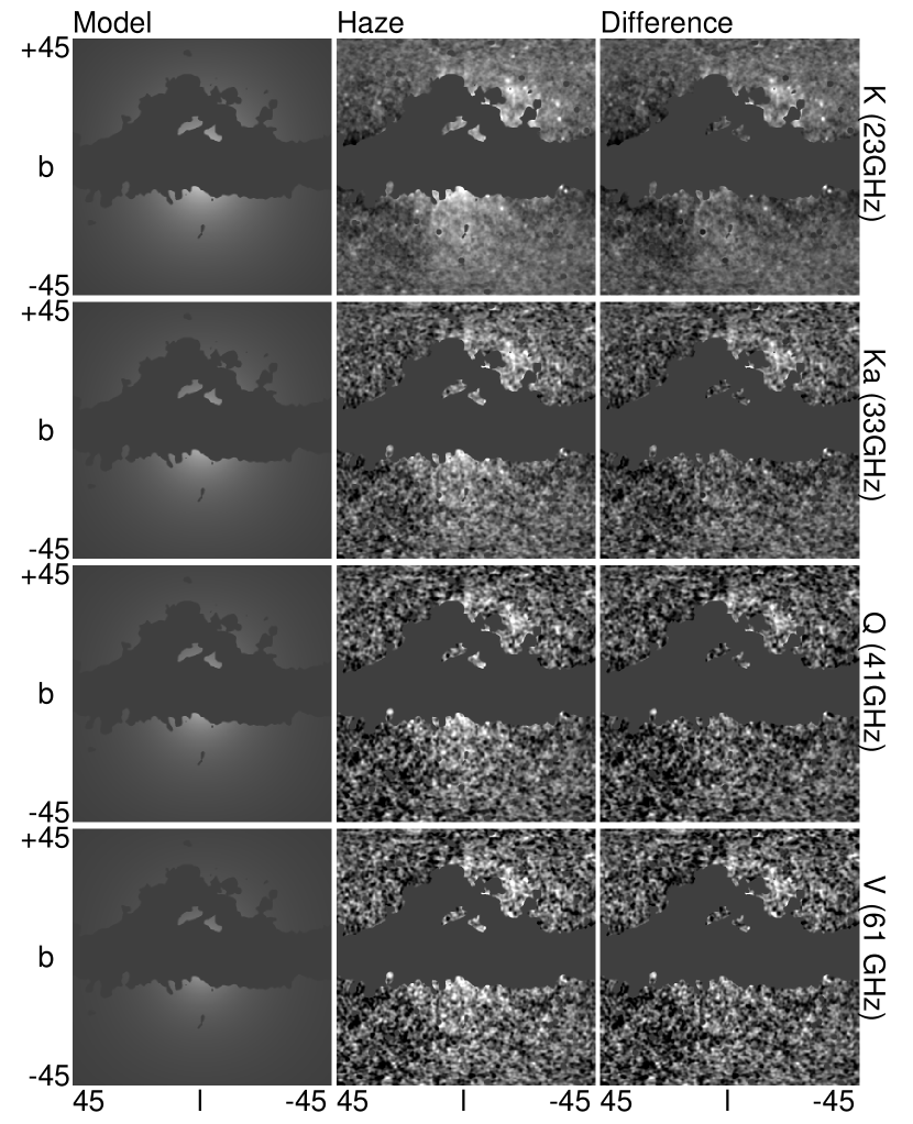
Figure 4: WMAP haze within $45^{\circ}$ of the Galactic center. Columns contain the emission from the model described in §4.2 (left), haze from Finkbeiner (2004) (center), and haze minus model (right). Each row corresponds to a WMAP band, with W-band absent due to lower signal-to-noise ratio. Pixels with known point sources, high extinction (more than 1 mag at H$\alpha$), or bright H$\alpha$($>25$ R) are masked. The color table in each image goes from $-2$ (black) to 6 (white) kJy/sr. One kJy/sr is $67\mu{\rm K}$ at $23{\rm~{}GHz}$.

4.4 X-rays and $\gamma$-rays

The hard $\gamma$ rays produced by inverse Compton scattering of starlight photons have an energy density similar to the microwave synchrotron emission (§3.4). The softer $\gamma$ rays from upscattered CMB photons are expected to be subdominant in the inner galaxy, but perhaps still detectable. Extensive searches for these signal have been carried out, and detections so far are suggestive.

The EGRET data from the Compton Gamma Ray Observatory at $0.1<E_{\gamma}<10{\rm~{}GeV}$ have long been claimed to show an excess of emission in the inner Galaxy over that expected from cosmic ray interaction with the ISM (Hunter et al.  1997; Strong, Moskalenko, & Reimer 2000). The hard $\gamma$ excess has remained enigmatic, though Strong et al.  (2000) were able to fit the observed spectrum by assuming a much flatter electron energy distribution above 1 GeV than that observed in the cosmic ray population near Earth. Recently, de Boer et al.  (2004) have considered dark matter annihilation as a source for these hot electrons and found reasonable agreement with $\gamma$ ray data and other constraints. Some of the de Boer et al.  assumptions about dark matter structure in the Galaxy may be controversial (a high degree of clumpiness is assumed), but it is interesting that both groups conclude that a very hot electron spectrum is present. Note that the absence of clumpiness would imply a lower $\gamma$ ray production, and would not violate the observations; there could be other sources as well.

An excess at lower energies observed by COMPTEL is at roughly the energy expected for scattered CMB photons; however the observed amplitude is higher by one or two orders of magnitude. The INTEGRAL $\gamma$ ray observatory has revealed numerous soft $\gamma$ point sources in the inner galaxy that could account for this emission (Lebrun et al.  2004). The fact that these sources are resolved leaves open the possibility that the upscattered CMB may be detected at a lower level with more sensitive instruments in the future. A detection of CMB scattering would be much easier to interpret than the putative starlight scattering, since the CMB photon density is isotropic and known. Starlight scattering calculations are significantly complicated by the fact that both energy and direction distributions must be known.

A great deal of work remains to tie the information provided by the observation of the WMAP microwave haze to the important constraints already imposed by the $\gamma$ ray data.

5 SUMMARY

We have attempted to constrain models of self-annihilating dark matter by searching for synchrotron emission from the annihilation products, assumed to be ultra-relativistic $e^{+}e^{-}$ pairs. We refer to the dark matter particle as the supersymmetric neutralino, and the mass as $m_{\chi}$, even though the results are of generic interest for any stable dark matter particle that annihilates into ultra-relativistic $e^{+}e^{-}$.

The Galactic emission found by Finkbeiner (2004) in the WMAP data in excess of the expected foreground Galactic ISM signal may be a signature of such dark matter annihilation. It has the spectrum, morphology, and total power expected for the simple model given above, which uses reasonable values for the parameters of the dark matter halo density, particle mass, and cross section; parameters that agree with other cosmological and accelerator constraints. Additional tests of this model are possible, given the X-rays and $\gamma$-rays produced by inverse-Compton scattered CMB and starlight photons, respectively. Current data are consistent with the model, but provides only loose constraints.

In addition to better X-ray and $\gamma$-ray data, sensitive microwave observations of other edge-on spiral galaxies (e.g. NGC 891 or NGC 4565) might reveal a similar signal, and verify these results. Tests of Milky Way satellite dwarf galaxies have also been suggested (Baltz & Wai 2004) but the signal from these may be too weak for current technology.

While the dark matter annihilation interpretation is exciting, it must be emphasized that other explanations are possible. A hard electron energy spectrum could be produced by novel physics around the supermassive black hole at the Galactic center. Although observations of other galaxies have not revealed such a flat spectrum of emission, they may have lacked the necessary resolution to separate the various emission components.

A more thorough investigation is required before declaring that the energetic population of electrons result from dark matter annihilation, and indeed, astrophysical observations alone are unlikely to make an entirely convincing case unless an annihilation line or sharp energy cut-off is found in $\gamma$ rays. Complementary data from the LHC (Ellis et al.  2004) and other particle accelerators will play an essential role in making the case for a new particle. The vastly improved data expected over the next few years, both experimental and observational, may finally provide an observational window into one of the great mysteries of modern cosmology, dark matter.

I am indebted to Jim Gunn and Bruce Draine for help and encouragement; David Schlegel, Robert Lupton, and Nikhil Padmanabhan for inspiration, technical advice, and helpful skepticism; Carl Heiles for advice on the Galactic B-field and other matters; Marc Davis for enlightening discussions; and Amber Miller for reminding me what an important problem dark matter annihilation is. Gus and Flora Schultz’s kind hospitality allowed me to work out the essentials of this problem while visiting their home in Berkeley. This research made use of the NASA Astrophysics Data System (ADS) and the IDL Astronomy User’s Library at Goddard. I am supported by NASA LTSA grant NAG5-12972, the Russell Fellowship, and the Cotsen Fellowship of the Society of Fellows in the Liberal Arts at Princeton University.

Appendix A TOTAL MILKY WAY ANNIHILATION

We assume the DM density in the Galactic halo obeys the NFW density profile,

$$\rho_{NFW}(r)=\frac{\rho_{0}r_{s}^{3}}{r(r^{2}+r_{s}^{2})}$$ (A1)

with a core radius $r_{s}=20{\rm~{}kpc}$ and $\rho_{0}=5.6\times 10^{-25}{\rm~{}g}{\rm~{}cm}^{-3}$, making the density in the Solar neighborhood $\rho(R_{\sun})=6.5\times 10^{-25}{\rm~{}g}{\rm~{}cm}^{-3}$ and $M_{gal}=2\times 10^{12}M_{\sun}$. The annihilation rate per volume is

$$\Gamma(r)=\left(\frac{\rho_{NFW}(r)}{m_{\chi}}\right)^{2}\langle\sigma_{A}v\rangle$$ (A2)

For Majorana particles, the annihilation rate is $\langle\sigma_{A}v\rangle n_{\chi}^{2}/2$, but in each annihilation, two particles are removed, which cancels the factor of 2 in the annihilation rate.

Note that the integral of $\Gamma(r)$ over all space (total number of annihilations per time) is

$$4\pi\int_{0}^{\infty}\Gamma(r)r^{2}dr=\pi^{2}\left(\rho_{0}/m_{\chi}\right)^{2}r_{s}^{3}\langle\sigma_{A}v\rangle$$ (A3)

which for the assumed parameters of $m_{\chi}=100{\rm~{}GeV}$, $\langle\sigma_{A}v\rangle=2\times 10^{-26}{\rm~{}cm}^{3}{\rm~{}s}^{-1}$, $\rho_{0}=5.6\times 10^{-25}{\rm~{}g}{\rm~{}cm}^{-3}$, and $r_{s}=20$kpc, is $4.6\times 10^{38}{\rm~{}s}^{-1}$ for the whole Galaxy. Assuming that the $e^{+}e^{-}$ pair creation rate is proportional to $\Gamma$, we define the efficiency $\eta$ as the number of relativistic $e^{-}$ (or $e^{+}$; hereafter simply called electrons) created per neutralino annihilation, so that the creation rate is $\eta\Gamma(r)$. The electron density is obtained by convolving this density function with the Green function obtained in Eq (12). In general, such a convolution looks like

$$h(E,r)=\int d\phi~{}d\theta r^{\prime 2}\sin\theta dr^{\prime}\Gamma(r^{\prime})G(|{\bf x}^{\prime}-{\bf x}|)$$ (A4)

and since both functions depend only on radius, we can assume $r$ to be on the $z$ axis such that the angle between $r$ and $r^{\prime}$ is $\theta$, then

$$n(E,r)=\int d\phi~{}d\theta r^{\prime 2}\sin\theta dr^{\prime}\Gamma(r^{\prime})G(\sqrt{r^{2}+r^{\prime 2}-2rr^{\prime}\cos\theta})$$ (A5)

Inserting the functions gives

$$n(E,r)=\frac{\rho_{0}^{2}r_{s}^{6}\langle\sigma_{A}v\rangle}{AE^{2}m_{\chi}^{2}(2\pi\sigma^{2})^{3/2}}\int d\phi~{}d\theta r^{\prime 2}\sin\theta dr^{\prime}\frac{1}{r^{\prime 2}(r^{\prime 2}+r_{s}^{2})^{2}}\exp(-(r^{2}+r^{\prime 2}-2rr^{\prime}\cos\theta)/2\sigma^{2})$$ (A6)

where $\sigma_{A}$ is the neutralino self-annihilation cross section, not to be confused with the Gaussian width $\sigma$. Integrating over $\theta$ and $\phi$ we get

$$n(E,r)=\frac{\rho_{0}^{2}r_{s}^{6}\langle\sigma_{A}v\rangle}{AE^{2}m_{\chi}^{2}(2\pi\sigma^{2})^{1/2}}\int dr^{\prime}\frac{1}{rr^{\prime}(r^{\prime 2}+r_{s}^{2})^{2}}\left[\exp\left(-\frac{(r-r^{\prime})^{2})}{2\sigma^{2}}\right)-\exp\left(-\frac{(r+r^{\prime})^{2})}{2\sigma^{2}}\right)\right]$$ (A7)

This quantity is number density per energy. Integrating $n(E,r)|dE/dt|$ over the whole Galaxy, we obtain a total annihilation rate of $4\times 10^{38}{\rm~{}s}^{-1}$

References

- Aloisio, Blasi, & Olinto (2004) Aloisio, R., Blasi, P., & Olinto, A. V. 2004, J. Cos. and Astroparticle Phys., 5, 7
- Baltz & Edsjö (1998) Baltz, E. A. & Edsjö, J. 1998, Phys. Rev. D, 59, 023511
- Baltz et al. (2002) Baltz, E. A., Edsjö, J., Freese, K., & Gondolo, P. 2002 Phys. Rev. D, 65, 063511
- (4) Baltz, E. A. & Wai, L. 2004, astro-ph/0403528
- (5) Baltz, E. A., & Gondolo, P. 2004, hep-ph/0407039
- Bennett et al. (2003) Bennett, C. L., et al. 2003, ApJS, 148, 97
- Bertone et al. (2002) Bertone, G., Sigl, G., & Silk, J. 2002, MNRAS, 337, 98
- Blasi et al. (2003) Blasi, P., Olinto, A. V., & Tyler, C. 2003, Astropart. Phys., 18, 649
- Cesarini et al. (2004) Cesarini, A., Fucito, F., Lionetto, A., Morselli, A., & Ullio, P. 2004, Astropart. Phys., 21, 267
- de Boer et al. (2004) de Boer, M., et al. 2004, astro-ph/0408272
- Draine & Lazarian (1998) Draine, B. T. & Lazarian, A. 1998, ApJ, 508, 157
- Edsjö & Gondolo (1997) Edsjö, J. & Gondolo, P. 1997, Phys. Rev. D, 56, 1879
- Ellis et al. (2000) Ellis, J., Falk, T., Olive, K. A., & Srednicki, M. 2000, Astropart. Phys., 13, 181
- Ellis et al. (2004) Ellis, J., Olive, K. A., Santoso, Y., & Spanos, V. C. 2004, hep-ph/0408118
- Finkbeiner et al. (1999) Finkbeiner, D. P., Davis, M., & Schlegel, D. J. 1999, ApJ, 524, 867
- (16) Finkbeiner, D. P. 2003, ApJS, 146, 407
- Finkbeiner, Langston, & Minter (2004) Finkbeiner, D. P., Langston, G. I., & Minter A. H. 2004, ApJ, in press and astro-ph/0408292
- Finkbeiner (2004) Finkbeiner, D. P. 2004, ApJ, in press, and astro-ph/0311547
- Gaustad et al. (2001) Gaustad, J. E., McCullough, P. R., Rosing, W., & Van Buren, D. 2001, PASP, 113, 1326
- Gondolo (1994) Gondolo, P. 1994, Nucl. Phys. Proc. Suppl., 35, 148
- Gondolo (2000) Gondolo, P. 2000, Phys. Lett. B, 494, 181.
- (22) Griest, K., & Seckel, D. 1991, Phys. Rev. D, 43, 3191
- Gunn et al. (1978) Gunn, J. E., Lee, B. W., Lerche, I., Schramm, D. N., & Steigman, G. 1978, ApJ, 223, 1015
- Haffner et al. (2003) Haffner, L. M., Reynolds, R. J., Tufte, S. L., Madsen, G. J., Jaehnig, K. P., & Percival, J. W. 2003, ApJS, 149, 405
- Hansen (2004) Hansen, S. H. 2004, MNRAS, 352, L41
- Haslam et al. (1982) Haslam, C. G. T., Stoffel, H., Salter, C. J., & Wilson, W. E. 1982, A&AS, 47, 1
- Heiles (1995) Heiles, C. 1995, ASP Conf. Ser. 80, 507
- Hinshaw et al. (2003) Hinshaw, G., et al. 2003, ApJS, 148, 135
- Hooper et al. (2004) Hooper, D., Taylor, J. E., & Silk, J. 2004, Phys. Rev. D, 69, 10, id. 103509
- Hunter et al. (1997) Hunter, S. D., et al. 1997, ApJ, 481, 205
- Jungman et al. (1996) Jungman, G., Kamionkowski, M., & Griest, K. 1996, Physics Reports, 267, 195
- Lebrun et al. (2004) Lebrun, F., et al. 2004, Nature, 428, 293
- Moore et al. (1998) Moore, B., Governato, F., Quinn, T., Stadel, J., & Lake, G. 1998, ApJ, 499, 5
- Navarro et al. (1997) Navarro, J. F., Frenk, C. S., & White, S. D. M. 1997, ApJ, 490, 493
- Page et al. (2003) Page, L., et al. 2003, ApJS, 148, 233
- (36) Press, W. H., Teukolsky, S. A., Vetterling, W. T., & Flannery, B. P. 1992, Numerical Recipes in C, 2nd edn. (Cambridge, UK: Cambridge University Press)
- Taylor & Cordes (1993) Taylor, J. H. & Cordes, J. M. 1993, ApJ, 411, 674
- SFD (98) Schlegel, D. J., Finkbeiner, D. P., & Davis M. 1998, ApJ, 500, 525 [SFD]
- Snowden et al. (1997) Snowden, S. L., et al. 1997, ApJ, 485, 125
- Spergel et al. (2003) Spergel, D. N., et al. 2003, ApJS, 148, 175
- Spitzer (1978) Spitzer, L. 1978, Physical Processes in the Interstellar Medium, Wiley, New York
- Stoehr et al. (2003) Stoehr, F., White, S. D. M., Springel, V., Tormen, G., & Yoshida, N. 2003, MNRAS, 345, 1313
- Strong et al. (2000) Strong, A. W., Moskalenko, I. V., & Reimer, O. 2000, ApJ, 537, 763
- Webber et al. (1992) Webber, W. R., Lee, M. A., & Gupta, M. 1992, ApJ, 390, 96