Cataclysmic variables from the Calán-Tololo-Survey – I. Photometric periods

Abstract

In a search for cataclysmic variables in the Calán-Tololo Survey we have detected 21 systems, 16 of them previously unknown. In this paper we present detailed time-series photometry for those six confirmed cataclysmic variables that show periodic variability in their light curves. Four of them turned out to be eclipsing systems, while the remaining two show a modulation consisting of two humps. All derived periods are below, or, in one case, just at the lower edge of the period gap.

1 Introduction

Cataclysmic variables (CVs) are close interacting binaries where a white dwarf primary accretes matter from a late-type main-sequence star. In absence of strong magnetic fields on the primary star, an accretion disc is formed, where the matter transferred from the secondary star spirals inwards until it is accreted by the white dwarf. For a comprehensive overview on CVs see Warner (1995).

The general evolution from the detached binary to the semi-detached state of a CV, and the subsequent long-term evolution to shorter orbital periods is thought to be driven by orbital angular momentum losses due to gravitational radiation and magnetic braking. Theoretical models based on this scenario imply that a CV should evolve down to an orbital period of $\sim$2 h in less than 10⁹ yr. The evolutionary lifetime of CVs near the shortest period ($\sim$80 min) should become drastically longer, as the thermal timescale of the secondary star becomes longer than the timescale of angular momentum loss by gravitational radiation. This behaviour should cause a “spike” in the orbital period distribution at the minimum period, as systems “pile up” at this point (Kolb, 1993; Stehle, Kolb & Ritter, 1997; Patterson, 1998). The theoretical predictions for this minimum period range up to $\sim$70 min (Kolb & Baraffe, 1999). Population synthesis calculations predict a space density $\sim$10^-4 pc^-3, with 99% of the CVs having periods shorter than 2 h, and 70% even having passed the turning point at the minimum period, with the now degenerate secondaries forcing an evolution towards longer orbital periods (Kolb, 1993; Stehle, Kolb & Ritter, 1997; Howell, Rappaport & Politano, 1997).

However, there exists a strong mismatch between these predictions and the actually observed sample. Observational estimates from large-area surveys derive a space density roughly a factor 10 lower than the predicted one (Patterson, 1998, and references therein). The observed period distribution of CVs shows only about half of the sources to have an orbital period below the period gap (Ritter & Kolb, 2003). The minimum of the observed period distribution is at $\sim$78 min, and there is no evidence of an enhancement in the number of sources close to this period (e.g., Barker & Kolb, 2003).

Alternative evolutionary models have been proposed (e.g., King & Schenker, 2002; Spruit & Taam, 2001). More significantly, the strength of the magnetic breaking, which is one of the fundamental ingredients in the standard model, appears to be much weaker than assumed (Andronov, Pinsonneault & Sills, 2003). However, the discrepancies described above can (at least partly) be the result of the observational biases affecting the sample of CVs, and this should be explored before discarding the standard (and in other respects quite successful) model.

In the standard model, the “missing” part of the population is thought to be dominated by low mass-transfer rate, short period dwarf novae, which are intrinsically very faint and show only very infrequent outbursts. Especially the relatively bright magnitude cut-off of large-scale surveys conducted hitherto (Palomar-Green, Edinburgh-Cape Blue Object Survey: Green et al., 1986; Stobie et al., 1997, respectively) make them strongly biased against these systems (Patterson, 1984; Shara et al., 1986).

The low mass-transfer rate dwarf novae we are looking for are expected to have a fairly blue continuum and strong hydrogen emission lines (see, e.g., Fig. 6 in Patterson, 1984). This emphasises the importance of using deep spectroscopic and photometric surveys for a systematic search for CVs. First results from such surveys have become available recently (e.g., the Hamburg Quasar Survey and the Sloan Digital Sky Survey; Gänsicke, Hagen & Engels, 2002; Szkody et al., 2002, 2003, respectively).

Starting in 1996, we have conducted a survey of candidate CVs selected from the Calán-Tololo Survey (CTS; see Maza et al., 1989, and references therein). The CTS has been designed to search for emission-line galaxies, quasars and galaxies with strong UV excess using objective prism plates. The spectra cover the wavelength range from $\sim$5300 Å down to the atmospheric cut-off. The survey includes 5150 deg², i.e. $\frac{1}{8}$ of the whole sky, in the southern hemisphere with $|b|\geq 20^{\circ}$. The typical limiting magnitude of the plates is $B_{J}\sim$18.5. About half of the CTS plates ($\sim$2100 deg²) had been examined in 1996, and those sources showing a blue continuum and hydrogen emission lines were selected as candidate CVs, yielding a sample of 59 objects. Follow-up observations identified 21 targets as definite CVs, including 16 previously unknown systems of which 4 CVs have been independently discovered by other surveys in the meantime (Tappert, Augusteijn & Maza, 2002).

In this paper we present detailed data for those CVs that show photometric modulations we believe to reflect the orbital periods. In future papers we will present time-resolved spectroscopy for the remaining CVs without previously known periods, and discuss the complete sample.

2 Observations and reductions

Table 1: The photometric observations. $n_{\rm data}$ gives the number of data points, $t_{\rm exp}$ the individual exposure time, $\Delta t$ the time range covered by the observations, and $V_{\rm av}$ the average $V$ magnitude during the run.

CTCV	R.A.J2000	DECJ2000	date	HJD	telescope	filter	$n_{\rm data}$	$t_{\rm exp}$ [s]	$\Delta t$ [h]	$V_{\rm av}$
J0549$-$4921	05:49:45.4	$-$49:21:56	1996-10-05	2 450 362	0.9 m	$V$	168	20	2.55	13.75
			1996-10-06	2 450 363	0.9 m	$V$	125	20	1.79	13.79
			1996-10-07	2 450 364	0.9 m	$V$	65	20	0.93	14.52
			1998-10-31	2 451 118	2.2 m	Gunn r	184	20	3.16	16.862
			1998-11-01	2 451 119	2.2 m	Gunn r	224	20	3.71	16.862
			1998-11-02	2 451 120	2.2 m	Gunn r	246	20	4.24	16.922
			1998-11-03	2 451 121	2.2 m	Gunn r	242	20	4.25	17.102
			1998-11-04	2 451 122	2.2 m	Gunn r	244	20	4.07	17.092
J1300$-$3052	13:00:29.1	$-$30:52:57	1996-04-23	2 450 197	0.9 m	$V$	74	120	6.44	15.721
			1996-04-24	2 450 198	0.9 m	$V$	154	60/120	4.88	15.531
			1997-04-28	2 450 567	0.9 m	$V$	306	30/60	6.76	18.671
J1928$-$5001	19:28:32.6	$-$50:01:34	1996-07-08	2 450 273	0.9 m	$V$	55	240/80	3.09	17.791
			1996-07-09	2 450 274	0.9 m	$V$	197	60	5.21	17.871
			1996-07-30	2 450 295	2.2 m	$V$	47	15/120	3.12	17.801
J2005$-$2934	20:05:51.2	$-$29:34:58	1996-10-05	2 450 362	0.9 m	$V$	169	30	2.90	15.91
			1996-10-07	2 450 364	0.9 m	$V$	164	30	2.81	15.92
J2315$-$3048	23:15:31.9	$-$30:48:46	1996-10-06	2 450 363	0.9 m	$V$	124	60	3.14	16.831
J2354$-$4700	23:54:20.4	$-$47:00:20	1996-10-03	2 450 360	0.9 m	$V$	24	240	1.78	18.871
			1996-10-04	2 450 361	0.9 m	$V$	66	180	3.83	19.021
(1) out-of-eclipse value, (2) Gunn $r$ magnitude

Table 2: The spectroscopic observations. Columns include the exposure time $t_{\rm exp}$, the wavelength range $\Delta\lambda$, the resolution $\Delta\lambda_{\rm FWHM}$, and the $V$ magnitude of the object at the time of the spectroscopic observations. The latter was determined from the acquisition frames.

CTCV	date	tel. / instr.	grism	slit [″]	$t_{\rm exp}$ [s]	$\Delta\lambda$ [Å]	$\Delta\lambda_{\rm FWHM}$ [Å]	V [mag]
J0549$-$4921	1996-10-09	1.54 m / DFOSC	11	1.5	5400	4340 – 9750	16	16.351(15)
J1300$-$3052	1996-07-31	2.2 m / EFOSC2	1	1.0	3600	3800 – 10500	30	18.730(33)
J1928$-$5001	1996-07-30	2.2 m / EFOSC2	1	1.0	3600	3800 – 10500	30	17.834(12)
J2005$-$2934	1996-07-30	2.2 m / EFOSC2	1	1.0	600	3800 – 10500	30	15.349(06)
J2315$-$3048	1996-07-30	2.2 m / EFOSC2	1	1.0	1200	3800 – 10500	30	16.960(21)
J2354$-$4700	1996-07-29	2.2 m / EFOSC2	1	1.0	2$\times$900	3800 – 10500	30	19.701
(1) spectrophotometric magnitude, not corrected for slit losses

Follow-up observations for all objects in the original sample were conducted at ESO telescopes in the form of optical spectroscopy, calibrated and time-series photometry. The dates and instruments used for the observations presented here are summarised in Tables 1 and 2.

The photometric data were obtained, with one exception, at the 0.9 m Dutch telescope, which was equipped with a 512$\times$512 pixel CCD. One observing run for CTCV J0549$-$4921 was conducted on the ESO/MPI 2.2 m using a test camera equipped with a Gunn r filter. Reduction was performed using IRAF routines for BIAS and flatfield correction. Aperture photometry was obtained with IRAF’s daophot package (Stetson, 1992), and the differential light curves were computed with respect to one or more suitable comparison stars that were checked for constancy.

Calibrated magnitudes for the systems were determined by single B, V, R exposures and subsequent comparison with suitable (i.e., non-variable) stars within the target’s CCD frame, which in return were calibrated with respect to Landolt (1992) standards. The colour information derived from the calibrated photometry will be analysed in the concluding paper.

The spectroscopic data were taken at the Danish 1.54 m and the ESO/MPI 2.2 m telescopes. After bias and flatfield correction the spectra were calibrated in wavelength using Helium-Neon (1.54 m telescope) and Helium-Argon (2.2 m telescope) lamps. Flux calibration was performed with respect to standard stars observed in the same night. The flux calibrated spectra were folded with Bessell (1990) filter curves to obtain photometric magnitudes. By comparison with the values derived from the acquisition frames (typically an exposure in the V or R filter) we determined the slit losses. Extreme values ranged from 0.2 mag (CTCV J1300$-$3052) to 1.1 mag (CTCV J0549$-$4921) with most values around 0.4 mag. Folding the spectra with more than one filter furthermore yielded photometric colours. Comparison with BVR photometry taken of the target in a similar brightness state showed an agreement in colour within 0.05 mag. For CTCV J2354$-$4700, no acquisition frame was available, hence the accuracy of the flux calibration could not be tested in this case.

3 Results

Figure 1: Spectra of the 6 CTCV sources as indicated. The absorption feature at $\lambda$7440 for CTCV J2354$-$4700 is an artifact.

Table 3: Equivalent widths (in Å) of the most prominent emission lines. A blank field indicates that this part of the spectrum was not covered with our observations, a ‘$-$’ that the corresponding line was not detected.

CTCV	Balmer				He I					He II	Fe II
	4102	4340	4861	6563	4471	5016	5876	6678	7065	4686	5173
J0549$-$4921			35	52	6	4	11	5	–	8	6
J1300$-$3052	15	24	47	110	–	–	12	–	–	–	–
J1928$-$5001	–	–	13	11	–	–	–	–	–	–	–
J2005$-$2934	25	33	66	219	6	8	18	5	9	–	8
J2315$-$3048	31	44	45	102	14	11	32	11	11	9	6
J2354$-$4700	13	41	58	104	22	21	40	21	18	–	–

For the majority of the systems we have measured the arrival times of humps or eclipses by fitting a polynomic function of second order to the periodic features. Since the uncertainties of the arrival times resulting from the parabolic fit are usually smaller than the real variation (e.g., due to changes in the profile of the feature caused by flickering), we have assumed identical uncertainties for all arrival times for a given source and scaled them to give a reduced $\chi^{2}=1.0$ for the fit to the arrival times to determine the ephemeris. For these sources with a well defined feature in their light curve, the cycle count between the times of arrival of the feature were unambiguous and the period could be derived directly.

In the two cases where this approach was not possible, we have computed periodograms based on the analysis-of-variance (AOV) algorithm (Schwarzenberg-Czerny, 1989) as implemented in MIDAS. A Monte Carlo simulation was applied in order to test the significance of alias peaks and to obtain an error estimation for the periods (Tappert & Bianchini, 2003; Mennickent & Tappert, 2001).

3.1 CTCV J0549$-$4921

The spectroscopic appearance of CTCV J0549$-$4921 is that of a typical dwarf nova, with moderately strong H and He I emission (Table 3). No signatures of the secondary star are detected (Fig. 1).

Time-series photometry of the system was taken on two occasions. During the first run in 1996, it proved to be in outburst, without showing any obvious periodic features (Fig. 2). The second run, in 1998, caught the CV in a $\sim$2.2 mag fainter state (we have no information on the colour $V-R$, but typical values for CVs are 0.1–0.5 mag; Echevarría, 1984). The light curves (Fig. 3) over 5 nights show little variation of the average value, and we therefore assume that the system was in, or close to, quiescence. The most prominent feature in these light curves is a periodic hump with an amplitude of $\sim$0.5 mag. A second, smaller and more distorted, hump is also present.

We have measured the arrival times of the maximum of the primary hump by fitting a second order polynomial function to the hump. The results are given in Table 4. The linear regression yields the ephemeris

$$T_{0}={\rm HJD}~{}2\,451\,118.8019(22)+0.080\,218(70)~{}E,$$ (1)

with $E$ giving the cycle number. Fig. 4 presents the 1998 light curve folded on this period.

Light curves containing variable double humps represent a phenomenon commonly seen in low mass-transfer rate dwarf novae (e.g., Patterson, 1980; Augusteijn & Wisotzki, 1997, for WZ Sge and BW Scl, respectively). Within our sample we find corresponding features also for CTCV J2005$-$2934, CTCV J2315$-$3048, and CTCV J2354$-$4700. In the latter two systems, the additional presence of an eclipse proves the orbital nature of the double hump. The usual explanation is that the humps correspond to the bright spot that is caused by the impact of the gas stream from the secondary star on the accretion disc, and which is seen at inferior (primary hump) and superior (secondary hump) conjunction. Within this picture, our (arbitrary) phase of the maximum of the primary hump in CTCV J0549$-$4921 should translate to an orbital phase of $\sim$0.8 with respect to superior conjunction of the white dwarf.

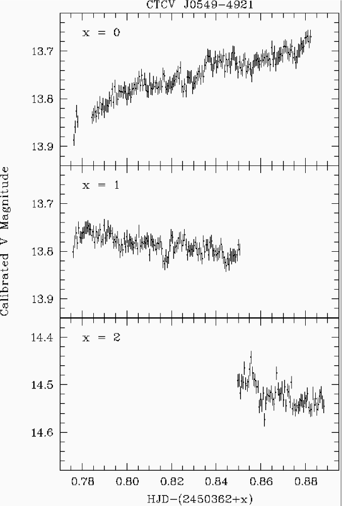
Figure 2: Light curves for the 1996 data of CTCV J0549$-$4921. Note that the relative magnitude range is the same for all plots.

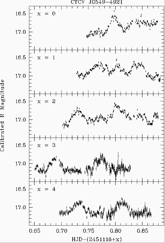
Figure 3: Light curves for the 1998 data of CTCV J0549$-$4921.

Table 4: Arrival times of the primary hump for CTCV J0549$-$4921. The uncertainties are those of the parabolic fit. The estimated uncertainty scaled with the reduced $\chi^{2}$ for all arrival times is $3.4\times 10^{-3}$ d (see text).

cycle	HJD
0	2 451 118.7983(05)
12	2 451 119.7701(13)
13	2 451 119.8417(08)
24	2 451 120.7306(09)
25	2 451 120.8063(07)
36	2 451 121.6889(12)
37	2 451 121.7729(19)
49	2 451 122.7310(14)
50	2 451 122.8122(18)

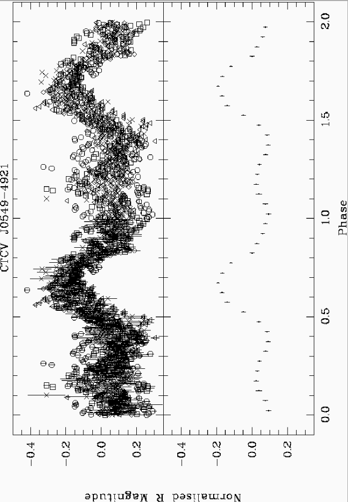
Figure 4: Light curve for CTCV J0549$-$4921 folded on $P$ = 0.080 239 d. The zero point of the phase has been set to the first data point. The symbols in the upper plot refer to the individual data sets from 1998-10-31 ($\circ$), 11-01 ($\Box$), 11-02 ($\triangle$), 11-03 ($\times$), and 11-04 ($\Diamond$). The error bars from phase 0 to 1 correspond to the photometric error as in Fig. 3. The lower plot shows the average light curve. The bin size is 0.05 phases.

3.2 CTCV J1300$-$3052

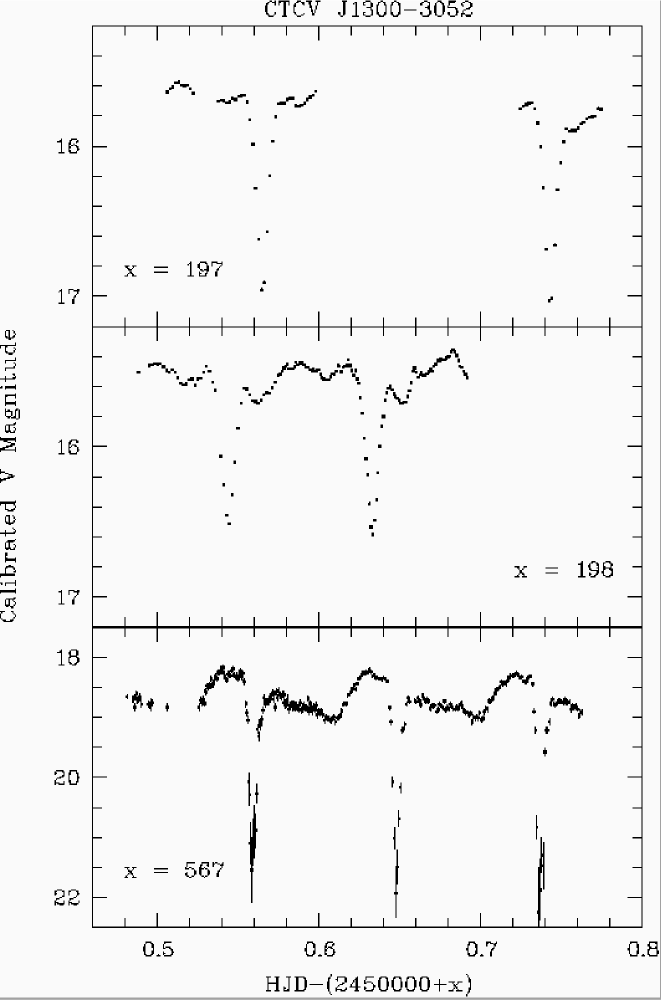
Figure 5: Light curves for CTCV J1300$-$3052 from 1996-04-23 (top), 1996-04-24 (middle), and 1997-04-28 (bottom). Note that the y-axis of the bottom plot has a different scale.

Table 5: Eclipse timings for CTCV J1300$-$3052. Due to the cycle ambiguity between both data sets, each refers to its individual zero point. The estimated error scaled by the reduced $\chi^{2}$ for the 1996 data amounts to $3.4\times 10^{-4}$ d. For the 1997 data, the errors resulting from the parabolic fit already gave reasonable residuals.

cycle	HJD
1996:
0	2 450 197.565 12(05)
2	2 450 197.743 57(06)
11	2 450 198.543 86(08)
12	2 450 198.633 29(08)
1997:
0	2 450 567.559 19(35)
1	2 450 567.648 05(22)
2	2 450 567.736 90(34)

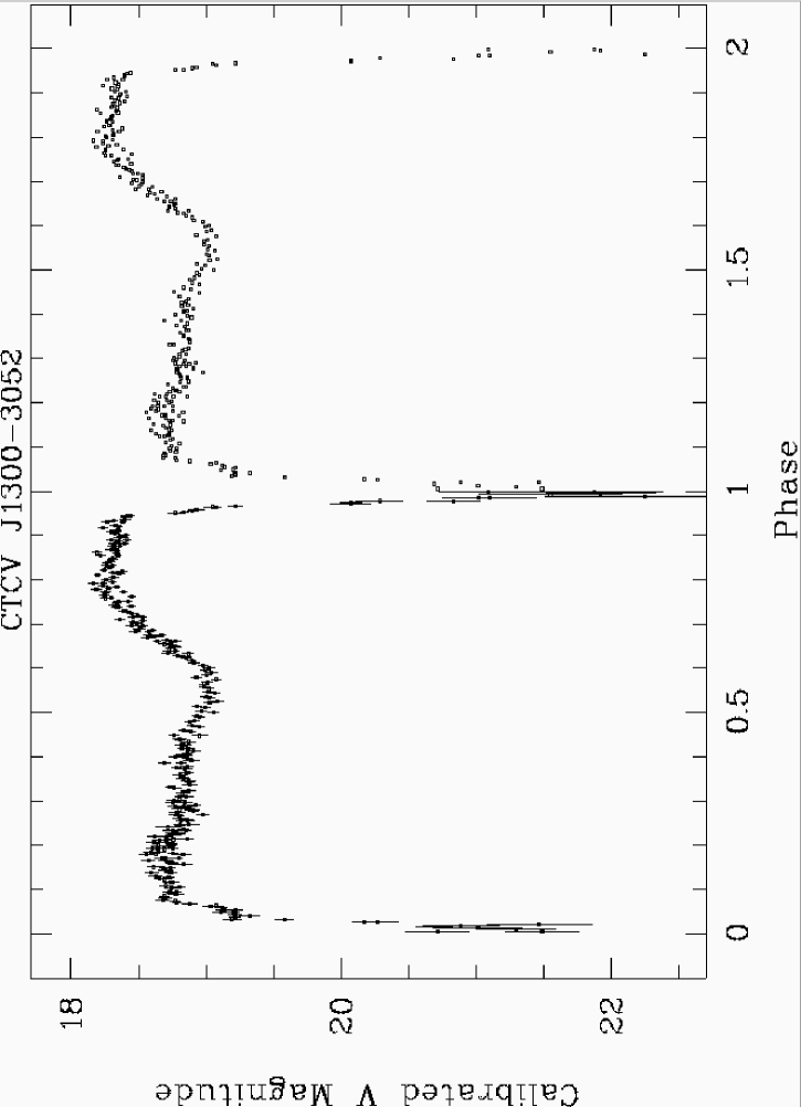
Figure 6: The 1997 light curve for CTCV J1300$-$3052 folded on the ephemeris given in Eq. 3.

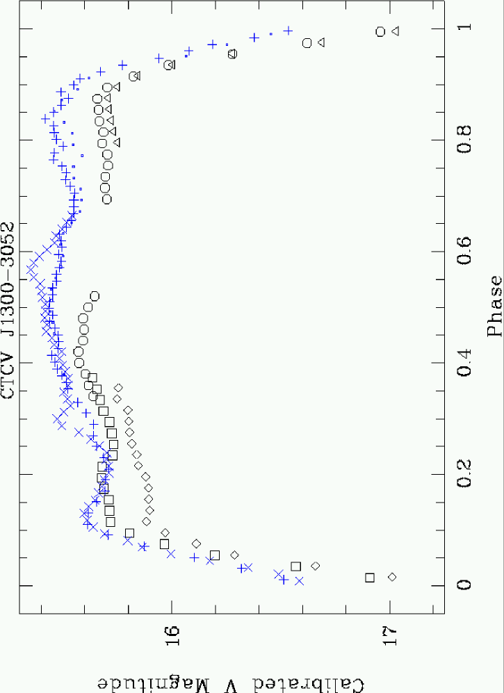
Figure 7: Phase folded outburst data CTCV J1300$-$3052 with respect to the ephemeris given in Eq. 2. Different symbols indicate different orbital cycles: $\circ$, $\Box$, $\triangle$, $\diamond$, for cycles $-1$, 0, 1, 2 (1996-04-23), and dot, $+$, $\times$, for cycles 10, 11, 12 (1996-04-24), respectively.

This object shows a composite spectrum with features from all three components: the typical strong emission lines from the accretion disc, which in the blue part of the spectrum are embedded in broad, shallow absorption troughs from the white dwarf primary, and the red continuum and absorption bands from the secondary star (Fig. 1). A rough comparison with standard star catalogues (Jacoby, Hunter & Cristian, 1984; Silva & Cornell, 1992) indicates an early M type for the latter.

We have observed the system photometrically in two different years, which proved it to be in a state of increased brightness during the first observing run in 1996. The light curves of both runs are given in Fig. 5. It shows the system with a $\sim$3 mag deep eclipse in quiescence. In the system’s high state the eclipse depth is diminished to $\sim$1.1 mag.

We have fitted second order polynomial functions to the eclipse data in order to determine the times of mid-eclipse. The results are given in Table 5. Unfortunately, a period analysis could not be performed on the combined data set, since the time span between the two observing runs proved too large for an unambiguous cycle count. Linear fits to the mid-eclipse timings for the individual runs yielded the ephemerises

$$T_{0}={\rm HJD}~{}2\,450\,197.565\,33(26)+0.088\,981(32)~{}E,$$ (2)

for the 1996 data, and

$$T_{0}={\rm HJD}~{}2\,450\,567.559\,19(29)+0.088\,85(24)~{}E,$$ (3)

for the 1997 data, with $E$ giving the cycle number. Within the errors, both periods are consistent with each other. This period places the system close to the lower edge of the CV period gap (e.g. Fig. 13 in Tappert & Bianchini, 2003).

The quiescence data folded on its ephemeris shows a ‘classical’ shape of a broad hump prior to eclipse (Fig. 6), very similar e.g. to that of U Gem (Krzeminski, 1965). The outburst light curve shows large, apparently irregular, variations from cycle to cycle (Fig. 7). A noteworthy feature of these data is the smaller depth and the larger width of the eclipse with respect to the quiescence data ($\sim$ 1 mag and 30 min for the full eclipse width compared to $\sim$ 3 mag and 19 min), as a consequence of increased disc luminosity and radius.

A more detailed study of the eclipse light curve and additional follow-up spectroscopic observations will be published elsewhere (Augusteijn et al., in preparation).

3.3 CTCV J1928$-$5001

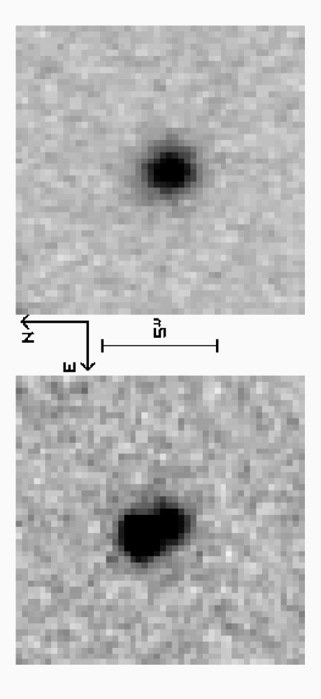
Figure 8: Out-of-eclipse (left) and mid-eclipse (right) $V$ image of CTCV J1928$-$5001 from 1996-07-30.

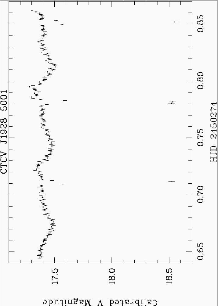
Figure 9: Light curve of CTCV J1928$-$5001 from 1996-07-09. The magnitudes represent the combined data from the CV and its close visual companion ($V$ = 18.5)

Table 6: Eclipse timings for CTCV J1928$-$5001 as measured with a polynomial fit of second order. The estimated uncertainty scaled by the reduced $\chi^{2}$ is $1.8\times 10^{-4}$ d.

cycle	HJD
$-$15	2 450 273.728 37(14)
$-$14	2 450 273.798 92(08)
$-$1	2 450 274.711 02(15)
0	2 450 274.781 39(08)
1	2 450 274.851 29(16)
297	2 450 295.624 47(09)
298	2 450 295.694 26(06)

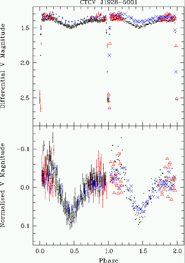
Figure 10: All three light curves of CTCV J1928$-$5001 folded on the ephemeris given in Eq. 4. The upper plots shows the differential magnitudes (the CV plus companion) to give an idea of the brightness variations of the system in its low state. The lower plot represents a close-up of the out-of-eclipse data.The latter light curves have been normalised individually by subtracting the corresponding out-of-eclipse average magnitude. In both plots the symbols $\times$ and $\triangle$ from phases 1 to 2 refer to the 1996-07-08 and 1996-07-30 data, respectively, while the dots represent the 1996-07-09 data. The error bars from phases 0 to 1 correspond to the individual photometric errors.

The spectrum of this object (Fig. 1) also shows contributions from multiple components. In the red part we see the signatures of the secondary star whose spectral type appears to be slightly later than M5V (Jacoby et al., 1984). The blue part is dominated by the Balmer absorption lines from the white dwarf primary. The source was identified as a Polar (or AM Her) type CV by follow-up spectroscopic and polarimetric observations which will be published elsewhere (Potter et al., in preparation).

The object is a close visual binary with a separation $\approx$ 2$\aas@@fstack{\prime\prime}$4. Additionally, the CV is a deeply eclipsing system (Figs. 8, 9). Mid-eclipse photometry of the companion gave $V$ = 18.52(1) mag, yielding out-of-eclipse values for the CV of $V$ = 17.7–18.0 mag. In order to estimate the mid-eclipse magnitude of the target, we subtracted the average PSF from the companion on an eclipse frame. Aperture photometry on the residual yielded $V$ = 21.05(30). Note, however, that the error is a purely photometric one, and does not take into account uncertainties in the PSF fitting or in the time deviation from true mid-eclipse, especially since the exact shape of the eclipse light curve is unknown. Therefore, deep mid-eclipse photometry will be needed to accurately determine the eclipse depth.

A linear fit to the timings of mid-eclipse (Table 6) yielded an ephemeris

$$T_{0}={\rm HJD}~{}2\,450\,274.781\,24(08)+0.070\,179(01)~{}E,$$ (4)

with the error of the zero cycle referring to the error of the linear regression. Fig. 10 shows the corresponding light curve.

3.4 CTCV J2005$-$2934

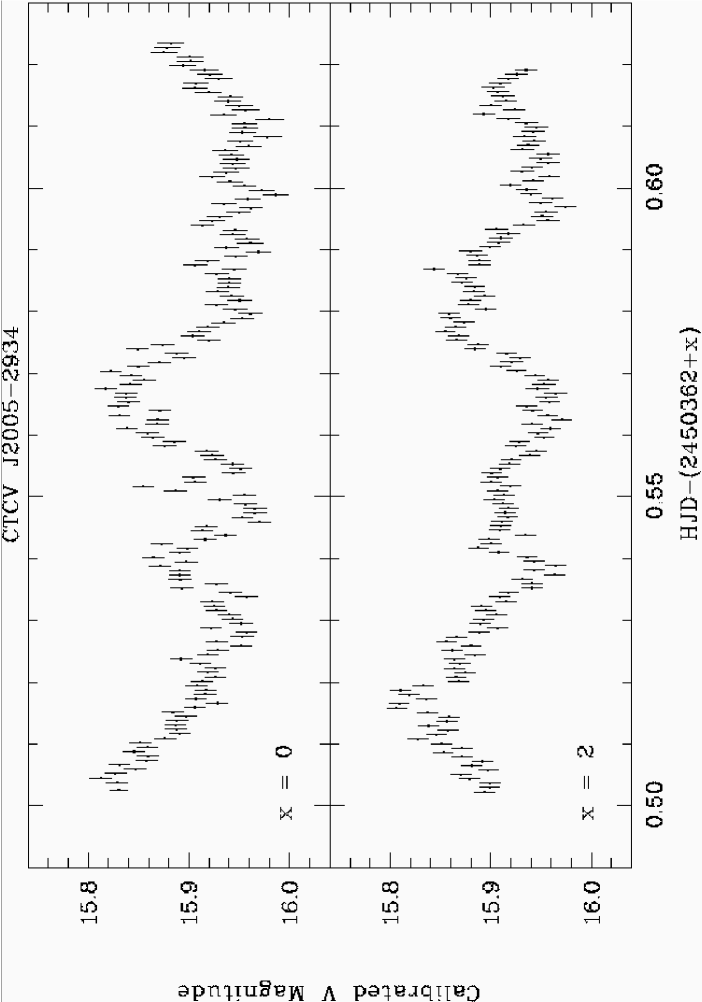
Figure 11: Light curves for CTCV J2005$-$2934 from 1996-10-05 (top) and 1996-10-07 (bottom).

Table 7: Frequencies $f$, corresponding periods $P$, and the discriminatory power $p_{d}$ from the Monte Carlo simulation on the CTCV J2005$-$2934 data.

$f$ [cyc d-1]	$P$ [d]	$p_{d}$	ID
14.901(15)	0.067 111(69)	0.000	$P_{1}$
15.398(05)	0.064 943(21)	0.091	$P_{2}$
15.902(09)	0.062 887(37)	0.637	$P_{3}$
16.401(04)	0.060 972(14)	0.272	$P_{4}$
16.892(07)	0.059 200(25)	0.000	$P_{5}$

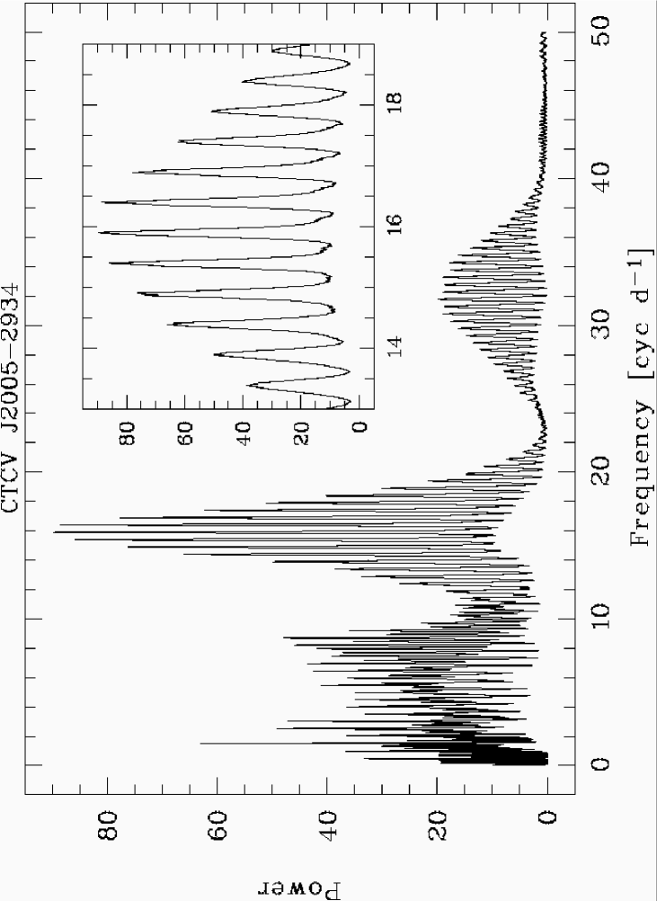
Figure 12: AOV periodogram for the CTCV J2005$-$2934 data. The inlet shows a close-up of the main peaks.

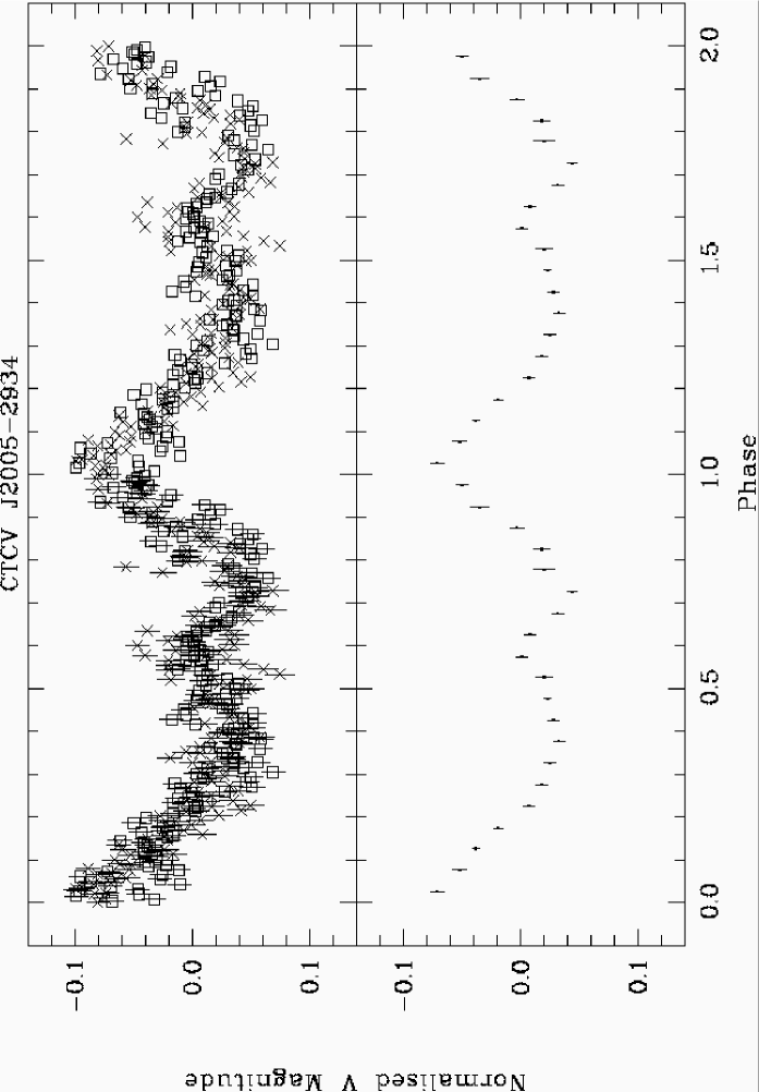
Figure 13: Normalised light curve for CTCV J2005$-$2934 folded on $P$ = 0.062 887 d. The zero point of the phase has been set to the first data point. The symbols in the upper plot refer to the individual data sets from 1996-10-05 ($\times$) and 1996-10-07 ($\Box$). The error bars from phase 0 to 1 correspond to the photometric error as in Fig. 11. The lower plot shows the average light curve. The bin size is 0.05 phases.

Although the spectrum of this system displays all basic ingredients of a typical dwarf nova, it is peculiar in that its H$\alpha$ line is unusually strong, especially in comparison to the other Balmer lines (Fig. 1, Table 3).

The photometric data was taken in two nights, with each data set spanning a very similar time range. The light curves are presented in Fig. 11. Other than in the CTCV J0549$-$4921 data, the time range and the number of covered humps are insufficient to use the arrival times of the principal hump to derive the period. Additionally the hump appears less constant in shape than the one of CTCV J0549$-$4921. After subtracting the nightly averages, we therefore applied the AOV algorithm to the combined data set. The corresponding periodogram shows a number of sharp peaks centred on $f\sim$16 cyc d^-1. For our Monte Carlo simulation we compared the five highest peaks. The corresponding frequencies and the resulting discriminatory power for a specific frequency over the other four are listed in Table 7. Thus, $P_{3}$ emerges as the most probable period, while we can certainly discard $P_{1}$ and $P_{5}$. However, especially $P_{4}$ still represents an important alias, and additional observations will be necessary to properly assign the orbital period.

In Fig. 13 we present individual light curves and the average one folded on the most probable period $P_{3}$. Phase-folding on $P_{2}$ or $P_{4}$ yields very similar scatter and basically identical phasing of the main features. The light curve is in principle similar to that of CTCV J0549$-$4921 in that it consists of two humps of different size. Their amplitudes, however, are only half as strong as those in CTCV J0549$-$4921, which could mean that CTCV J2005$-$2934 is seen at a somewhat lower inclination. Using the same interpretation for the nature of these humps, orbital phase $\sim$0.8 should correspond to our arbitrary phase 0.03 for the maximum of the primary hump.

3.5 CTCV J2315$-$3048

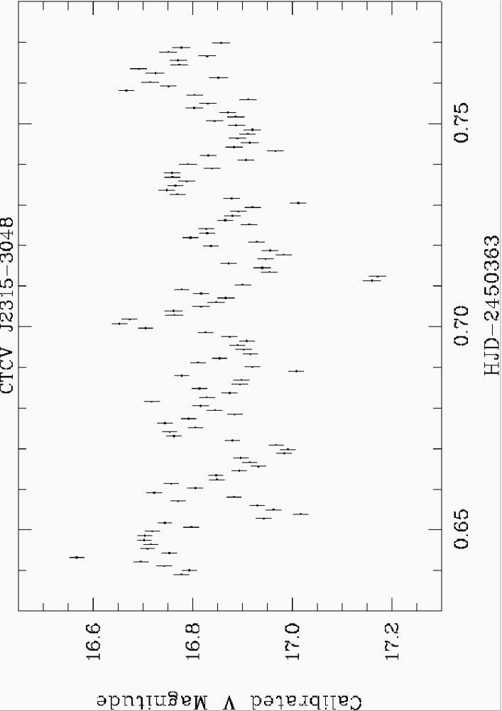
Figure 14: Light curve for CTCV J2315$-$3048 from 1996-10-06.

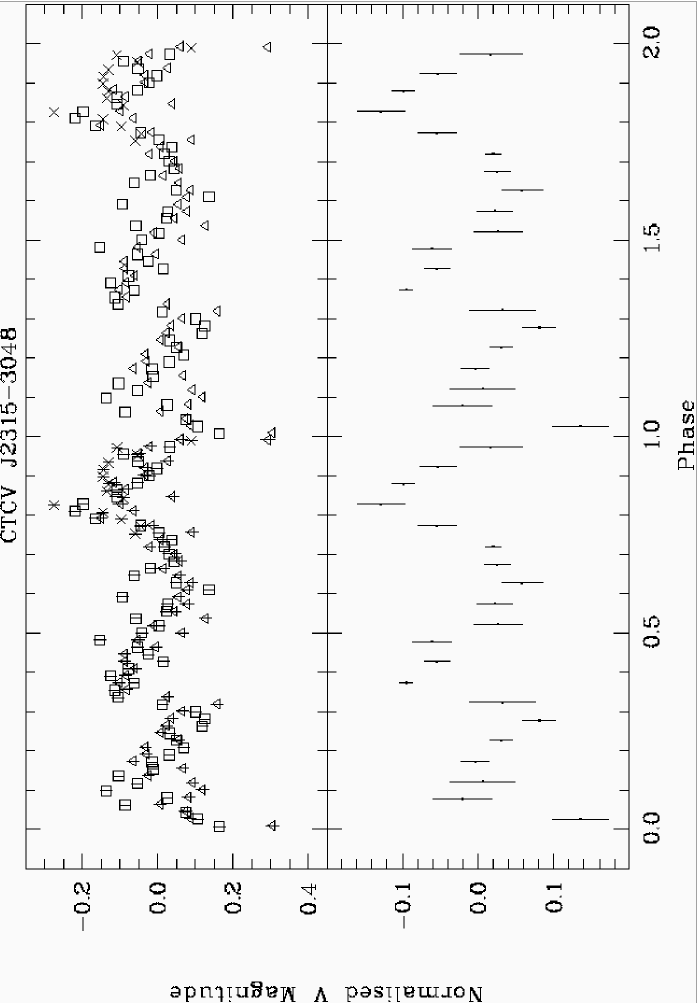
Figure 15: Light curve for CTCV J2315$-$3048 folded on the ephemeris given in Eq. 5. The data have been normalised by subtracting a polynomial of second order. For the fit the eclipse data and the first hump were excluded. The data set in the upper plot has been divided into three parts, each corresponding to a different orbital cycle ($-$2 = $\times$, $-$1 = $\Box$, 0 = $\triangle$). The error bars from phase 0 to 1 correspond to the photometric error as in Fig. 14. The lower plot shows the average light curve with a bin size of 0.05 phases. The y-scale has been set in such a way to enable direct comparison to Fig. 3 of Chen et al. (2001).

This object shows a very typical spectrum of a dwarf nova in quiescence with strong emission lines of the H and He series (Fig. 1, Table 3). It has been independently discovered as the ROSAT source 1RXS J231532.3$-$304855 (Schwope et al., 2000) and in the Edinburgh-Cape Blue Object Survey as EC 23128$-$3105 (Chen et al., 2001). The latter authors derive an orbital period $P$ = 0.0584(2) d from time-resolved spectroscopy. They furthermore find a strong orbital modulation in a photometric light curve from 1991, and report a possibly transient feature resembling a shallow eclipse.

We have observed the system in one night 5 years later, with the data set covering roughly 2.25 orbital cycles. The light curve is presented in Fig. 14. The AOV periodogram yields two broad peaks corresponding to $P$ and $P$/2. Since with our data set we cannot obtain the accuracy of Chen et al. (2001) in the period determination, we have used their value to compute a phase-folded light curve (Fig. 15).

The presence of strong flickering has a distorting effect within an individual orbital cycle. However, in our average light curve we find the same principal features as in Chen et al.’s data (their Fig. 3). Of special interest is that we also detect an eclipse-like dip just after the primary maximum. Chen et al. report that this feature is not found in all their light curves. Also in our data the first eclipse feature is much less evident than the second one. By simply taking the average in time for the two data points that define the second eclipse, and which have the same magnitude within the errors, we obtain an ephemeris

$$T_{0}={\rm HJD}~{}2\,450\,363.711\,90(53)+0.058\,4(2)~{}E,$$ (5)

with the periodic term taken from (Chen et al., 2001). The error for the zero cycle corresponds to half of the separation of the two data points, and is therefore likely to be somewhat overestimated.

3.6 CTCV J2354$-$4700

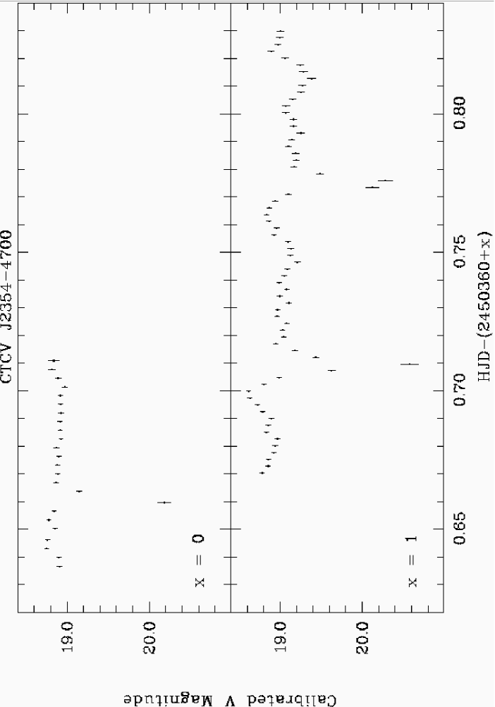
Figure 16: Light curves for CTCV J2354$-$4700 from 1996-10-03 (top) and 1996-10-04 (bottom).

Table 8: Times of mid-eclipse for the CTCV J2354$-$4700 data.

cycle	HJD
0	2 450 360.661 45(56)
16	2 450 361.709 80(47)
17	2 450 361.775 80(46)

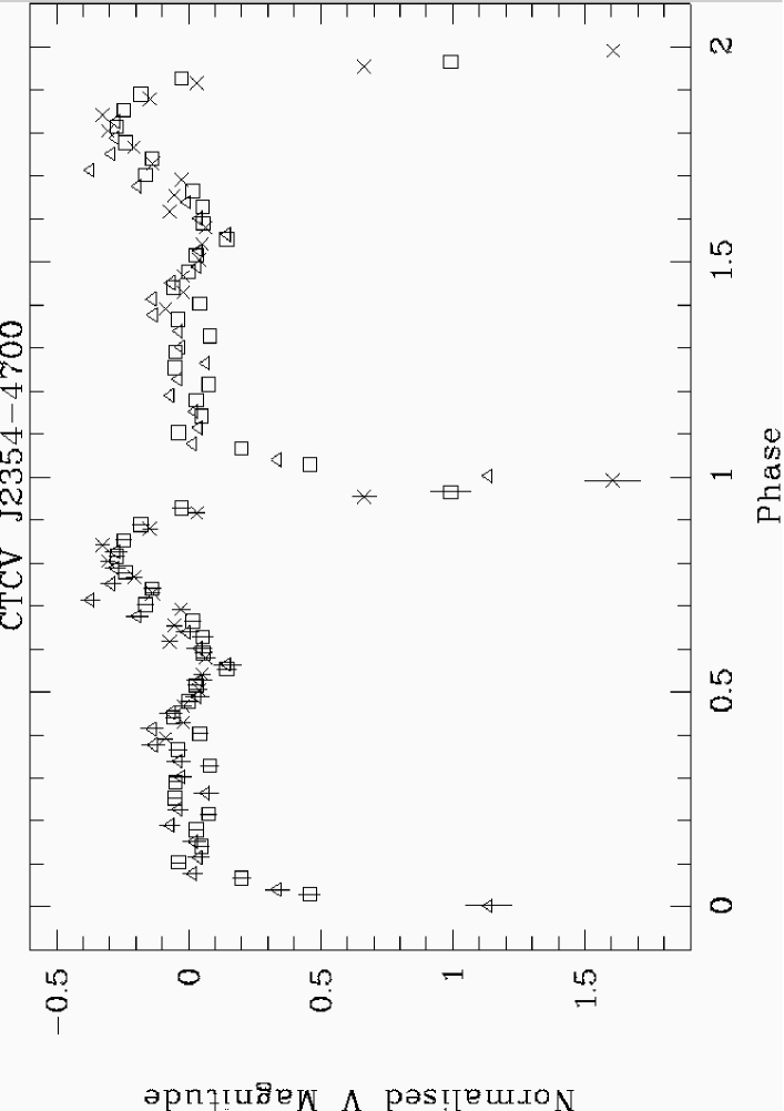
Figure 17: The 1996-10-04 light curve of CTCV J2354$-$4700 folded on the ephemeris given in Eq. 6. The symbols in the plot refer to different orbital cycles (15 = $\times$, 16 = $\Box$, 17 = $\triangle$). The data have been normalised by subtracting a linear fit to the data (excluding humps and eclipses) with a slope of 2.59 mag d^-1.

The spectrum of this object is very similar to the one of CTCV J2315$-$3048, i.e. of a dwarf nova in quiescence (Fig. 1).

CTCV J2354$-$4700 was observed on two subsequent nights. Fig. 16 presents the resulting light curves, and Table 8 lists the times of mid-eclipse which were obtained by fitting a second order polynomial to the eclipse data.

A linear fit to these times yielded the ephemeris

$$T_{0}={\rm HJD}~{}2\,450\,360.661\,43(56)+0.065\,538(39)~{}E.$$ (6)

Both data sets for CTCV J2354$-$4700 show steadily declining light curves. Linear fits, excluding the humps and eclipses, yielded slopes of 1.05(49) mag d^-1 and 2.59(24) mag d^-1 for the 1996-10-03 and the 1996-10-04 data, respectively. Since on both dates the average magnitudes are very similar, it is clear that at least the value for the first night does not reflect the system’s behaviour over a longer period of time. Therefore, either the CV has undergone some slow, non-orbital, variations between the two nights, or the decline (perhaps in both nights) is artificial. For the 1996-10-04 data the airmass has been continuously increasing (from 1.05 to 1.58), and 3 of the 5 stars in the average comparison light curves are very red with $B-V\geq 0.9$, raising the suspicion that the decline may be due to differential extinction. However, light curves for the target computed with respect to the bluest ($B-V=0.4$) and the reddest ($B-V=1.5$) comparison star yield nearly identical decline rates. Computing the difference light curve of the two comparison stars with the most extreme colour coefficient we do find the signature of differential extinction in the form of a decline of $\sim$0.1 mag d^-1 for both nights (in the first night, the standard deviation of the slope even still includes a constant light curve). In the average light curve, this effect can be assumed to be even less pronounced. We therefore do not find any indication for an artificial origin of the observed decline, but due to the rather limited amount of data we have to leave the question on the cause of this apparent long-term variation to be answered by future studies.

In order to fold the data on the above ephemeris, we have subtracted the linear decline from the 1996-10-04 data. Fig. 17 presents the such normalised, phase-folded, light curve. Its shape is very similar to that of CTCV J1300$-$3052, although in the latter both the amplitude of the hump and the depth of the eclipse are roughly twice as strong, suggesting a lower inclination for CTCV J2354$-$4700.

4 Summary

Table 9: Summary of the orbital periods for the six CVs.

object	$P$ [d]	$P$ [h]	notes
CTCV J0549$-$4921	0.080 218(70)	1.9252(17)
CTCV J1300$-$3052	0.088 981(32)	2.135 54(77)	[1]
CTCV J1928$-$5001	0.070 179(01)	1.684 296(24)	[1]
CTCV J2005$-$2934	0.062 887(37)	1.5093(09)	[2]
CTCV J2315$-$3048	0.058 4(2)	1.402(05)	[1], [3]
CTCV J2354$-$4700	0.065 538(39)	1.5729(09)	[1]
[1] eclipsing, [2] most probable alias, [3] period from Chen et al. (2001)

We have presented the results of time-series photometry for six CVs that were detected in the Calán-Tololo Survey, and where we find photometric variations that we believe to be modulated with the orbital period. For five of the systems we derived this previously unknown period, and in the case of CTCV J2315$-$3048 we have confirmed the existence of an eclipse, which has been previously discussed as a possibly transient feature Chen et al. (2001). The resulting periods for all systems are summarised in Table 9.

Appendix A Finding charts

We here present 5′$\times$5′ finding charts for the 6 CVs.

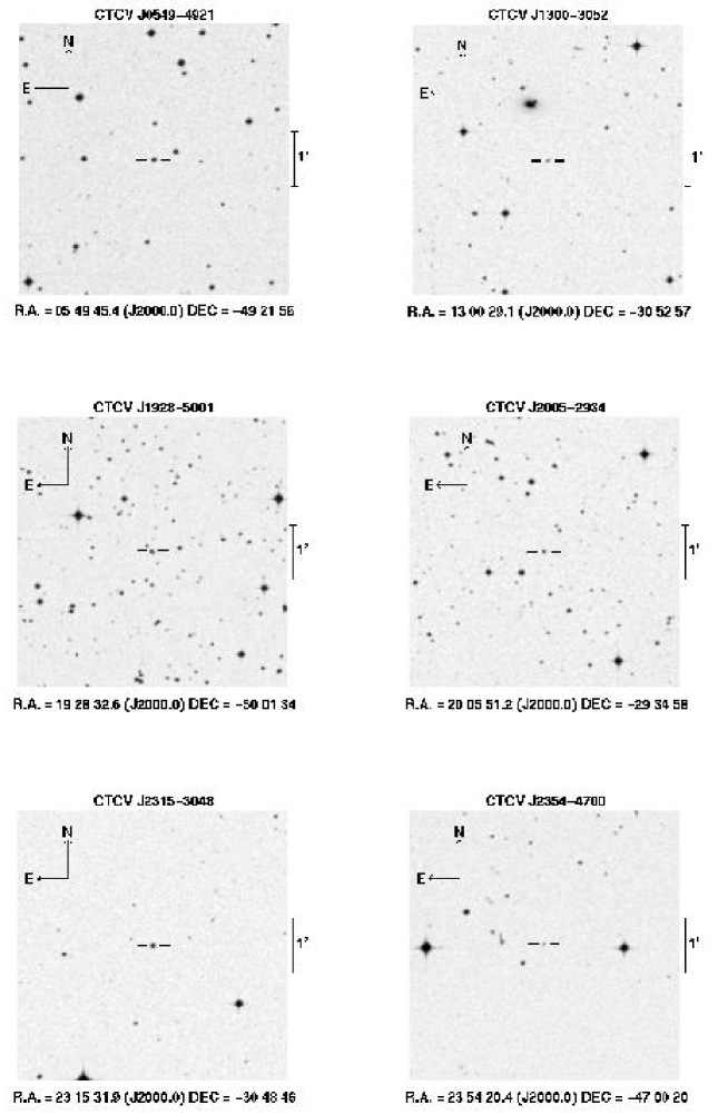
Figure 18: Finding charts from the Digitized Sky Survey.

References

- Andronov et al. (2003) Andronov N., Pinsonneault M., Sills A., 2003, ApJ, 582, 358
- Augusteijn & Wisotzki (1997) Augusteijn T., Wisotzki L., 1997, A&A 324, L57
- Barker & Kolb (2003) Barker J., Kolb U., 2003, MNRAS, 340, 623
- Bessell (1990) Bessell M. S., 1990, PASP, 102, 1181
- Chen et al. (2001) Chen A., O’Donoghue D., Stobie R. S., Kilkenny D., Warner B., 2001, MNRAS, 325, 89
- Echevarría (1984) Echevarría J., 1984, Rev. Mex. Astron. Astrof., 9, 99
- Gänsicke et al. (2002) Gänsicke B.T., Hagen H.-J., Engels D. 2002, in Gänsicke B. T., Beuermann K., Reinsch K., eds, The Physics of Cataclysmic Variables and Related Objects, ASP Conf. Ser., 261, p. 190
- Green et al. (1986) Green R. F., Schmidt M., Liebert J., 1986, ApJS, 61, 305
- Howell et al. (1997) Howell S. B., Rappaport S., Politano M., 1997, MNRAS, 287, 929
- Jacoby et al. (1984) Jacoby G. H., Hunter D. A., Cristian C. A., 1984, ApJS, 56, 257
- King & Schenker (2002) King A. R., Schenker K., 2002, in Gänsicke B. T., Beuermann K., Reinsch K., eds, The Physics of Cataclysmic Variables and Related Objects, ASP Conf. Ser., 261, p. 233
- Kolb (1993) Kolb U., 1993, A&A, 271, 149
- Kolb & Baraffe (1999) Kolb U., Baraffe I., 1999, MNRAS, 309, 1034
- Krzeminski (1965) Krzeminski W., 1965, ApJ, 142, 1051
- Landolt (1992) Landolt A. U., 1992, AJ, 104, 340
- Marsh (2000) Marsh T. R., 2000, New Astron. Rev., 44, 119
- Maza et al. (1989) Maza J., Ruiz M. T., Gonzalez L. E., Wischnjewsky M., 1989, ApJS, 69, 349
- Mennickent & Tappert (2001) Mennickent R.E., Tappert C., 2001, A&A 372, 563
- Patterson (1980) Patterson J., 1980, ApJ, 241, 235
- Patterson (1984) Patterson J., 1984, ApJS, 54, 443
- Patterson (1998) Patterson J., 1998, PASP, 110, 1132
- Ritter & Kolb (2003) Ritter H., Kolb U., 2003, A&A, 404, 301
- Schwarzenberg-Czerny (1989) Schwarzenberg-Czerny A., 1989, MNRAS, 241, 153
- Schwope et al. (2000) Schwope A., Hasinger G., Lehmann I., et al., 2000, Astron. Nachr., 321, 1
- Shara et al. (1986) Shara M.M., Livio M., Moffat A. F. J., Orio M., 1986, ApJ, 311, 163
- Silva & Cornell (1992) Silva D. R., Cornell M. E., 1992, ApJS, 81, 865
- Spruit & Taam (2001) Spruit H. C., Taam R. E., 2001, ApJ, 548, 900
- Stehle et al. (1997) Stehle R., Kolb U., Ritter H., 1997, A&A, 320, 136
- Stetson (1992) Stetson P. B., 1992, in Worrall D. M., Biemesderfer C., Barnes J., eds, Astronomical Data Analysis Software and Systems I, ASP Conf. Ser., 25, p.291
- Stobie et al. (1997) Stobie R. S., Kilkenny D., O’Donoghue D., et al., 1997, MNRAS, 287, 848
- Szkody et al. (2002) Szkody P., Anderson S. F., Agüeros M., et al., 2002, AJ, 123, 430
- Szkody et al. (2003) Szkody P., Fraser O., Silvestri N., et al., 2003, AJ, 126, 1499
- Tappert & Bianchini (2003) Tappert C., Bianchini A. 2003, A&A, 401, 1101
- Tappert et al. (2002) Tappert C., Augusteijn T., Maza J., 2002, in Gänsicke B. T., Beuermann K., Reinsch K., eds, The Physics of Cataclysmic Variables and Related Objects, ASP Conf. Ser., 261, p.299
- Warner (1995) Warner B., 1995, Cataclysmic Variable Stars, Cambridge University Press