The Origins and Evolutionary Status of B Stars Found Far From the Galactic Plane I: Composition and Spectral Features

Abstract

The existence of faint blue stars far above the galactic plane, which have spectra that are similar to nearby Population I B stars, present several interesting questions. Among them are: Can a Population I B star travel from the disk to a position many kiloparsecs above the plane in a relatively short main sequence lifetime? Is it possible that single massive star formation is occurring far from the galactic plane? Are these objects something else masquerading as main sequence B stars? This paper (the first of two) analyzes the abundances of a sample of these stars and reveals several which are chemically similar to nearby Population I B stars while others clearly have abundance patterns more like those expected in BHB or PAGB stars. Several of those with old evolved star abundances also have interesting features of note in their spectra. We also consider why this sample does not have any classical Be stars and identify at least two nearby solar metallicity BHB stars.

1 Introduction

1.1 History

Faint blue stars at high galactic latitudes were first discovered in a survey conducted by Humason & Zwicky (1947). Soon after, Bidelman (1948) brought attention to a number of stars of early spectral type with heliocentric velocities greater than 100 km/s. Their faint apparent magnitudes (sizable distances) and high velocities led to the conclusion that these objects, which appear at low spectroscopic dispersions to be Population I stars, are in fact a part of the galactic halo.

There are currently three basic explanations for B stars found far from the galactic plane:

1. “Normal” massive Population I stars ejected from the galactic disk,

2. Older evolved stars (i.e. blue horizontal branch (BHB) or post asymptotic giant branch (PAGB) stars), or

3. Young massive stars formed in situ in the galactic halo.

We will now briefly discuss the history of these scenarios and characteristics that can be used to distinguish which stars have been affected by each scenario.

Greenstein & Sargent (1974) studied a sample of faint blue stars within 30 degrees of the galactic poles and found that 50 of the 189 objects surveyed at low spectroscopic dispersion were indistinguishable from normal Population I B stars. The radial velocities of these stars implied that twenty of them took longer than their projected main sequence lifetimes to travel from the disk to their present location. Since in situ star formation in the galactic halo seemed an impossible scenario to them, Greenstein & Sargent (1974) concluded that several of these seemingly normal Population I main sequence stars are in fact low mass evolved stars.

Subsequent photometric and spectroscopic surveys continued to identify significant numbers of high galactic latitude B stars as ”normal” Population I stars until Tobin (1987) showed that many of these studies could have mistaken older evolved stars for young main sequence stars. Armed with this information, researchers interested in post asymptotic giant branch (PAGB) stars saw this population of B stars far above the galactic plane as a potential boon to the study of rare and poorly defined stages of stellar evolution (McCausland et al., 1992). The possibility that many of these stars could be old evolved stars masquerading as “normal” Population I stars is the impetus for this research and other studies including Magee et al. (2001), Ramspeck, Heber, & Edelmann (2001), and Ramspeck, Heber, & Moehler (2001). These new studies, realize the importance of using many different analysis tools in concert since no one indicator alone has proven able to characterize the B stars found far from the galactic plane.

The observed spectra of stars are largely a function of effective temperature and surface gravity. Unfortunately, these parameters alone are not enough to distinguish high mass hydrogen burning main sequence stars from low mass post asymptotic giant branch (PAGB) stars or low mass helium burning blue horizontal branch (BHB) stars. Hot PAGB stars may traverse one of many evolutionary tracks with effective temperatures and surface gravities that are comparable to stars on the main sequence. BHB stars with effective temperatures between 10,000 K and 20,000 K, where the horizontal branch crosses the main sequence, are also easily confused with main sequence B stars (Tobin, 1987). In this regime, stars that otherwise have the same atmospheric parameters can have large differences in mass and luminosity depending on their evolutionary status. Temperatures and gravities can be determined for these stars by various means (photometry, absolute flux fitting, fitting of spectral features) but their masses, distances, and intrinsic luminosities remain in most cases only an educated guess. Fortunately, their photospheric compositions and full space velocities provide additional clues the origin and evolutionary stage of a star.

Runaway Population I stars ejected from the galactic disk should have photospheric elemental abundances which are, for the most part, indistinguishable from their parent population (nearby Population I B stars in the galactic disk). At the same time, they should have space velocities which allow them to traverse large distances from the galactic plane to their present location within their main sequence lifetime.

Older evolved stars should exhibit photospheric abundances patterns which are markedly different from Population I stars due to their initial composition and processes which occurred earlier in their lifetimes such as mixing and dust grain formation. Many older evolved stars are also less luminous than main sequence stars with the same effective temperature. Overestimating their luminosity and photometric distance by assuming that they are main sequence stars will inflate their space velocities causing them to stand out kinematically from other populations.

The final possibility is that these are massive stars which have formed far out of the galactic disk. Massive stars formed in situ in the halo should have photospheric elemental abundances which are consistent with the composition of gas clouds found far from the galactic plane (i.e. Intermediate Velocity Clouds (IVCs) or High Velocity Clouds (HVCs)). These stars should kinematically belong to the halo population and need not have velocities which allow them to have traveled from the disk to their present location within their main sequence lifetime.

We undertook a multifaceted study which is designed to try to unravel the various possibilities for these stars. Due to the extent of the work, it has been divided into two papers for publication.

1. This paper analyzes the photospheric elemental abundances and other spectral characteristic of a sample of high galactic latitude B stars.

2. The second paper will analyze the kinematics of the stars in the sample and then use a combination that data and the data from this paper to classify the origin and nature of each star in the sample.

1.2 Distinguishing Stellar Populations Using Relative Photospheric Abundance Analysis

In order to compare the abundances of stars they must be subjected to the same analysis because absolute abundances are subject to systematic errors which are difficult to quantify. This means that a control sample must be analyzed if one wants to make a valid comparison between the stars in a sample and another stellar population. Many past studies of high latitude B stars neglected to use a control sample in their analysis and as such were unable to make strong conclusions about the chemical composition of those stars relative to nearby B stars. In contrast, more recent work by Hambly et al. (1997), Rolleston et al. (1999), and Magee et al. (2001) have compared the abundances of B stars found far from the galactic plane with control samples of nearby Population I B stars. These studies have shown that many of the high galactic latitude B stars have abundances which are strikingly similar to nearby Population I B stars, with some small indication of slight deficits or enhancements in a few elements.

BHB stars have average rotational velocities which are significantly lower than main sequence stars with the same effective temperatures (Peterson, 1993; Peterson, Rood, & Crocker, 1995). Peterson (1983) showed that stars on the horizontal branch in globular clusters have projected rotational velocities (vsin(i)) smaller than 40 km/s, as opposed to main sequence B stars which have average rotational velocities on the order of 100 km/s (Abt, Levato, & Grosso, 2002). While fast rotating BHB stars appear to be ruled out, main sequence B stars with small vsin(i) are not (for example HR 6165, $\gamma$ Peg, HR 8768). For the time being, we will ignore vsin(i) as a selection criterion so that the final selection of runaway B stars is unbiased with respect to this parameter. Detailed abundance analysis should be able to differentiate between these populations since conventional wisdom holds that the abundance pattern of elements in BHB stars should be significantly different from main sequence stars due to their advanced evolutionary state.

The abundances of evolved stars differ from those of main sequence B stars for a variety of reasons including:

• Initial composition,

• Enhancement or depletion of specific elements by nuclear processing, and

• Depletion of refractory elements by dust grain formation.

It is not uncommon to find stars in similar advanced evolutionary states which have differing abundance patterns due to variation in the processes which combined to create the composition of their stellar atmospheres. For the most part, the atmospheres of main sequence stars are influenced by their initial composition, although mixing and other factors may have a small effect. Still there is relatively little variation in the abundances of B stars recently formed in the solar neighborhood between 6 kpc and 10 kpc from the galactic center where the disk abundance gradient appears to be almost flat (Kilian, 1992; Gies & Lambert, 1992; Daflon, Cunha, Smith, & Butler, 2003; Andrievsky, Luck, Martin, & Lépine, 2004). It is reasonable to assume that most runaways which we observe at high galactic latitudes come from this region since most of their ejection velocity is probably directed perpendicular to the galactic plane keeping them close to the galactocentric radius which they formed at. Therefore, under ideal conditions abundance anomalies are a certain way to separate high mass main sequence stars from low mass evolved stars.

There is the unexcluded possibility that some high latitude B stars are the product of ongoing in situ star formation in the galactic halo. van Woerden (1993) and Christodoulou, Tohline, & Keenan (1997) report that the conditions thought to exist in intermediate and high velocity clouds (IVCs and HVCs) found high above the galactic plane are conducive to the formation of individual massive stars. Even if the conditions exist in IVCs and HVCs for ongoing star formation, there is no observational evidence of star formation in these clouds (Hopp, Schulte-Ladbeck, & Kerp, 2003; Willman et al., 2002; Ivezic & Christodoulou, 1997; Hambly et al., 1996). Star formation apparently is occurring under what are thought to be similar environmental conditions in the H I bridge between the LMC and SMC (Christodoulou, Tohline, & Keenan, 1997) and Comerón, Torra, Méndez, & Gómez (2001) report signs of star formation occurring in the halo of the edge-on spiral galaxy NGC 253. However, it should be noted that NGC 253 is a starburst galaxy so those results may not be applicable to the Milky Way. Wakker (2001) found that HVCs and IVCs have significantly metal poor chemical compositions. Therefore, any star formed in the halo would have to have photospheric abundances which are comparable to these clouds. As a result, we expect that B stars formed in situ in the halo should be metal poor by a factor of ten to one hundred with respect to B stars formed in the disk.

2 The Sample & Data

Forty nine (49) high galactic latitude B stars were identified in the Hipparcos catalog (Turon et al., 1997) for this study (Table 1). The sample is restricted to stars above declination -30 degrees which can be observed with the McDonald Observatory 2.1-m Struve Reflector using the Sandiford Echelle Spectrograph (McCarthy, Sandiford, Boyd, & Booth, 1993). Thirty two (32) are from the Greenstein & Sargent (1974) survey list of “normal” B stars. The other seventeen (17) stars are B stars from the Hipparcos Catalog (Turon et al., 1997) which have spectroscopic parallaxes and galactic latitudes placing them at least one kiloparsec above the galactic plane. Contamination of the sample by nearby subdwarfs was minimized by rejecting any star not classified by Greenstein & Sargent (1974) which has a significant Hipparcos geometric parallax ($\pi>2\sigma_{\pi}$). Some of the stars in the sample are not strictly at what some may consider to be high galactic latitude, but all of them are suspected to be a significant distance above the galactic plane.

In addition to the sample of study, three control samples were designated to serve as comparisons for the abundance analysis (Table 2). An abundance control sample of nearby Population I B stars was taken from the Yale Bright Star Catalog (Hoffleit, 1982). Small vsin(i) was favored in the nearby Population I sample because weak metal lines can be measured to higher accuracy in stars with smaller rotational broadening. A few more rapid rotators were included as well because a number of the stars in the sample of study have significant vsin(i) values. In most cases, stellar rotation has no significant effect on the abundance analysis. However, the most rapid rotators were excluded because at the target signal to noise (100:1) it is exceedingly difficult to measure lines in stars rotating in excess of 150 km/s. Two additional samples were selected to serve as comparisons in the abundance analysis: a sample of blue horizontal branch (BHB) stars was selected from the brighter objects listed in Greenstein & Sargent (1974) and a sample of post asymptotic giant branch (PAGB) stars of spectral type B9 or hotter was taken from a list provided by Luck (1998).

2.1 Observations & Reductions

High resolution spectra (R=60000) were obtained for all the stars in the control samples and forty three (43) of the stars in the main sample on six separate observing runs using the McDonald Observatory 2.1-m Struve Reflector with the Sandiford Echelle Spectrograph (McCarthy, Sandiford, Boyd, & Booth, 1993). Constraints on observing time meant that no spectra were observed for six stars in the sample (HD 8323, BD +16 2114, BD +49 2137, HD 121968, HD 125924, and BD +20 3004). The abundances of three of the stars observed were not analyzed because of obstacles that prevented their spectra from being measured: Feige 23 (had no measurable metal lines), BD +13 3224 (is a short period pulsating helium dwarf V652 HER), AG +03 2773 (is not a B star, see section 3.1). Even though these stars are excluded from the abundance analysis, they are included in other aspects of this study.

All the spectra were reduced and extracted using IRAF . The extracted spectra were continuum normalized, wavelength calibrated, and had equivalent widths and feature depths determined using the ASP software package of Luck (2001a). Some of the spectra were binned in order to increase the signal to noise of the data. After combining exposures and binning the data almost all of the spectra have a signal to noise of at least 100:1.

The equivalent widths were measured interactively by direct integration of the line profiles in the spectra. Only single unblended lines and lightly blended lines which could be de-blended were measured. The wavelength overlap of the Echelle orders makes it possible to measure the equivalent width of some lines on two or more adjacent orders. Typically, multiple measures of the same feature varied on the order of the noise level (see below). Individual measures of the equivalent width from adjacent orders and multiple observations were averaged to improve accuracy. Lines with observed equivalent widths which are smaller than the noise level in the data have been dropped from the analysis. The minimum measurable equivalent width is calculated from the noise contribution to the integrated line profile as the area of a Gaussian with the depth of the noise level and the FWHM of the lines in the spectra. Expressing the FWHM as a function of line width in velocity space (vsin(i)) and normalizing the signal to one yields:

$$\sigma_{EW}=\frac{3\lambda_{0}}{2(S/N)}\times\frac{vsin(i)}{c}$$ (1)

Where $\lambda_{0}$ is the wavelength of the line center and c is the speed of light. Therefore, a spectrum with the target S/N of 100 at 4500 Å has 2.3 mÅ of noise for each 10 km/s of line broadening. This means that typically the noise level ranges from a few milliangstroms for the spectrum of a narrow lined star up to 50 mÅ or more for a spectrum with low S/N and very broad lines.

For quality control, the equivalent widths measured from spectra of HR 6165 by this study were compared with those measured by Hambly et al. (1997) and Kilian & Nissen (1989). There is a negligible average difference ($0.3\pm 4.5$ mÅ) between the equivalent widths of the 93 lines measured both this study and Hambly et al. (1997). The small systematic difference ($4.6\pm 4.8$ mÅ) between the equivalent widths measured by both this study and Kilian & Nissen (1989) is most likely attributable to a difference in spectral resolution and subjective uncertainty associated with continuum setting. In any case, 4.6 mÅ is not significant compared to the noise level encountered in most of the data.

3 Stellar Atmospheric Parameters

3.1 Effective Temperature & Surface Gravity

The effective temperature and surface gravity of the stars in the samples were determined by combining results obtained from a number of different photometric indices and flux fitting methods. The photometry is taken from GCPD database (Mermilliod, Mermilliod, & Hauck, 1997) and the references cited therein. The photometry is corrected for interstellar extinction using the E(B-V) values listed in Table 3 (references are listed in the table) and extended to other wavelengths and colors using excess ratios derived from the interstellar extinction curve of Fitzpatrick (1999) (assuming $\frac{E(B-V)}{A_{V}}=3.1$).

The results of the photometric temperature and gravity relations are presented in Table 3. The Johnson (B-V) color-temperature relation (Napiwotzki, Schoenberner, & Wenske, 1993) should be considered only a crude estimate because the large band-passes and effective wavelengths of the Johnson UBV filters make them poorly suited to measure blackbody curves of B stars. The Strömgren temperature relation of Napiwotzki, Schoenberner, & Wenske (1993) was selected over other Strömgren methods because, unlike other relations, it is independent of the $H\beta$ index which can be influenced unpredictably by Balmer line emission which is common in B stars. The Geneva Photometry for each star was processed using the temperature and surface gravity relation of Kunzli, North, Kurucz, & Nicolet (1997).

Surface gravities were also measured from the Balmer line profiles by comparing the observed spectra to synthetic profiles generated using ATLAS9 and BALMER9 (Kurucz, 1993) assuming the effective temperatures derived from the photometry. The wings of the Balmer lines cover most of the Echelle orders so the continua are set by rescaling the continua from the previous or subsequent orders without a hydrogen line. The estimated accuracy of this method is $\pm 0.25$ dex or better.

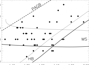
Figure 1: A plot of the effective temperatures and surface gravities of the program stars (diamonds) compared to the position of the zero age (solid line) and terminal age (dotted line) Main Sequence (Tout, Pols, Eggleton, & Han, 1996; Hurley, Pols, & Tout, 2000), the zero age (solid line) and terminal age (dotted line) Horizontal Branch (Dorman, Rood, & O’Connell, 1993), and a representative post-asymptotic branch track for a 1.5 M_☉ star (dashed line) (Schoenberner, 1979). All the tracks represented are for solar metallicity ([Fe/H] = 0).

The results from the individual temperature and gravity relations were combined into single values. The greatest weight given to the effective temperatures determined using Geneva photometry with the Strömgren temperature estimate being a close second. For surface gravities, the highest weights were given to values derived from Balmer line fitting and/or Geneva photometry. Most importantly, the temperature and gravity of each star (Table 4) were accepted only if the observed spectrum could be reasonably synthesized by MOOG (see section 4.2) using an atmospheric model with those parameters. It should be noted that the spectra of stars with significant rotational broadening are reasonably fit by a wider range of atmospheric parameters than stars with sharp spectral features. Therefore, there is less certainty in the atmospheric parameters of more rapidly rotating stars. Figure 1 shows the effective temperature and surface gravity of each star plotted in relation to the main sequence and horizontal branch.

Unfortunately BD +61 996, HIP 41979 and AG +03 2773 have only (B-V) photometry and the temperatures derived from that data do not produce synthetic spectra which match the observed spectra. For HIP 41979 and BD +61 996, the temperatures from the (B-V) data and the gravities from the Balmer profiles were used as starting points to determine the effective temperatures by matching the features in the observed spectra to a series of synthetic spectra produced by MOOG. AG +03 2773 has a unique spectrum with many strong rotationally broadened absorption lines making it nearly impossible to set the continuum. Furthermore, the (B-V) color (0.275) is not consistent with a star of its spectral type (B5) and interstellar extinction along the line of sight is insufficient to explain this discrepancy. The most likely explanation is that this star is actually a late type A or early type F star which has been misclassified.

NLTE effects may impact the photometric effective temperature and surface gravity relations since most of them rely on theoretical colors calculated from stellar atmospheres which assume LTE. The role of NLTE effects with respect to these calibrations is more significant in hotter ($\geq$ 20000 K) and/or lower gravity stars. Kilian, Becker, Gehren, & Nissen (1991) found that temperature estimates for B stars made from the Strömgren [c1] index are systematically 2000 K cooler than temperature estimates made from H I and Si III lines after accounting for NLTE effects. However, Vrancken, Butler, & Becker (1996) found that Kilian, Becker, Gehren, & Nissen (1991) had overestimated this difference by at least 300 K to 500 K. Fortunately, Sigut (1996) found no similar offset between NLTE temperature estimates and the Napiwotzki, Schoenberner, & Wenske (1993) [u-b] temperature relation employed in this study. The exact effect of NLTE on derived stellar parameters is an unresolved subject of ongoing study. The best course of action is to be conscious of the fact that, particularly in hot super giants, there may be a tendency to overestimate the stellar effective temperature.

3.2 Microturbulence

The microturbulent velocity ($\xi_{t}$) is determined by finding the value at which the slope of abundance versus equivalent width for the lines of a given atomic species is zero. Species with many lines that span a large range of equivalent widths are the best barometers of microturbulence. For hotter B Stars, O II, N II, and Si III have well populated curves of growth that are ideal for determining the microturbulence. For cooler B stars, Fe II, Cr II, and Ti II are good species to use. Theoretically, the microturbulent velocity should be the same for all species. However in practice, there is sometimes a discrepancy between the results measured from different elements and ionization stages. Of particular note, in early type B super giants Si III sometimes indicates a smaller LTE microturbulence value than O II (McErlean, Lennon, & Dufton, 1998; Vrancken, 1997). McErlean, Lennon, & Dufton (1999) suggest that in these circumstance the Si III $4550\mbox{\AA}$ triplet gives a better answer since the lines in the triplet cover a range of strengths and are from the same multiplet, thus less susceptible to systematic errors in the atomic data.

For this study the microturbulent velocity obtained by balancing the Si III $4550\mbox{\AA}$ triplet has been given preference. When the Si III $4550\mbox{\AA}$ triplet is not available, a consensus between the other species with the best populated curves of growth is used. In the cases where fewer than three lines of any species were measured, making it impossible to determine the microturbulent velocity, the value used is “borrowed” from another star with a similar effective temperature and gravity. The microturbulent velocities assigned to each star and the species used to determine them are listed in Table 4.

The LTE microturbulence values for B stars are typically on the order of 5 km/s to 10 km/s or more. Microturbulent velocities of this magnitude dominate the broadening parameter for most elements since at 20000 K the thermal velocities of hydrogen and iron atoms are 12.8 km/s and 1.7 km/s respectively. Typically the microturbulent velocity can be determined to better than $\pm 2$ km/s which translates into an uncertainty in the abundances of less than 0.10 dex. However, this uncertainty may be higher for stars using “borrowed” microturbulence values, especially for the abundances of heavier nuclei with slower thermal velocities where the microturbulence thoroughly dominates the line broadening parameter. In extreme cases the abundances may be affected by several tenths of a dex.

3.3 Projected Rotational Velocity

The vsin(i) was determined for each star by synthesizing a piece of spectrum broadened by the method of Gray (1976) using several different broadening parameters and visually picking the one that best fit the observed profiles. The Si III $4550\mbox{\AA}$ triplet or another piece of spectrum containing at least on prominent unblended absorption line were used to determine the best fit vsin(i) for each star listed in Table 4. The error in each vsin(i) value is about 10% with a best possible accuracy of about $\pm 1$ km/s for the narrowest line stars. A comparison of the vsin(i) values measured in this study with other sources shows a good agreement (Figure 2).

As part of this work, we wish to distill an sample of Population I runaways which is unbiased with regards to rotational velocity. Therefore, we are not using vsin(i) as a criterion to classify the stars in the sample. The distribution of rotational velocities in the sample will be discussed further in Paper II after each star has been assigned a final classification based on both its photospheric abundances and space velocity.

4 Abundance Analysis

4.1 Stellar Model Atmospheres

An extensive grid of plane parallel, LTE stellar photospheric models covering the range of stellar atmospheric parameters in B stars was calculated using ATLAS9 (Kurucz, 1993) at steps of 250 K effective temperature and 0.25 dex surface gravity using the standard solar abundance ODFs (Opacity Distribution Functions). We conducted numerical experiments which showed that the metallicity of the ODFs used to calculate the atmospheric models could be changed by up to 2.0 dex and that the constant microturbulent velocity of the models could be varied by up to 15 km/s with no significant effect on the abundance analysis. The models were calculated using a constant microturbulent velocity of 5 km/s for models hotter than 9000 K and a velocity of 2 km/s for cooler models. Note that convection can be ignored in most cases since it does not contribute significantly to energy transport in the atmospheric models of B stars.

Uncertainty in the parameters which define the model atmospheres directly translate into uncertainty in the abundances. Each atomic species is affected differently by these uncertainties. Minor species which represent less than 5% of the population at the level of maximum contribution are very sensitive to temperature and pressure. Therefore, it is minor species which are most affected by perturbations in the structure of the models. These effects can be quantified by comparing the relative abundances calculated from the same equivalent widths using different models. The differences in abundances of selected elements resulting from variation of the atmospheric parameters are given in Table 5. In all cases, the minor species show the largest variation with respect to the temperature and gravity of the selected model. On a fairly consistent basis, the calculated offsets are well within the typical standard deviation of the abundances calculated from the measured equivalent widths.

4.2 LTE Radiative Transfer Code

This study used the LTE radiative transfer codes LINES and MOOG (Sneden, 1973; Luck, 2001b). LINES is used to convert equivalent widths for single transitions into abundances while MOOG is used to synthesize and fit line profiles with one or more components. Both codes were optimized to perform abundance analysis in the B star temperature regime. The dominant line broadening mechanism in B stars is the quadratic Stark effect. Our experiments showed that the Cowley (1971) method is best able to reproduce the observed line profiles so it was installed as the method used to calculate the Stark broadening parameters in both codes.

Both MOOG and LINES passed a number of consistency checks. A piece of spectrum synthesized by MOOG is comparable to the same spectrum synthesized by SYNTHE (Kurucz, 1993). LINES is able to successfully recover the abundances for equivalent widths synthesized by MOOG as well as reasonably reproduce the abundance analysis results of Gies & Lambert (1992) and Hambly et al. (1997) from the data given in those publications.

4.3 LTE versus NLTE

NLTE effects, which are normally characterized as atomic level population perturbations relative to LTE, influence both individual line formation and the overall structure of a stellar atmosphere. These effects are more significant for some lines than others. Kilian (1994) found that at the $\pm$(0.1 to 0.2) dex level there is no difference between the absolute abundances calculated using LTE assumptions versus NLTE calculations. Whereas, Daflon, Cunha, Butler, & Smith (2001b) found that the difference between LTE and NLTE abundances in B stars depend on the atomic species. They showed that differences between LTE and NLTE derived abundances of C III and Al III are negligible while N II, O II, and Si III NLTE abundances are 0.1 to 0.2 dex higher than LTE abundances and Mg II NLTE abundances are up to 0.25 dex lower than LTE abundances. However, these differences are less significant in a relative abundance analysis where the abundances of the control sample are affected in the same manner as the sample of study.

4.4 Line and Atomic Data

The atomic transition data used in this analysis was obtained from the NIST online atomic database and the sources listed therein. The lines used in the analysis were selected from the measured absorption features as the ones that do not show large a abundance spread in the nearby Population I control sample (see the next section). The lines and atomic data used to model each transition are listed in Table 8 (available only in the electronic version of this paper).

4.5 Abundances of the Population I Control Sample

The absolute abundances measured for the stars in the Population I control sample are given in Table 6. The abundances of each element are measured using the dominant species in each star. The average abundances of this control sample compare favorably with the results from a variety of other studies (also Table 6). Note that the observed abundances of some elements in B stars are depressed relative to the established solar values. We assure the reader that this is a universally observed phenomenon which should not cause undue concern especially in the case of a relative abundance analysis (see references at the bottom of Table 6).

4.6 Abundances Measured Relative to the Control Sample

It is easiest to measure the relative abundances between two stars with the same atmospheric parameters because then the only variable which they do not have in common is their composition. In a perfect universe there would be one star that we could observe as a standard which all other stars could be compared to (i.e. the Sun). However in reality, stars cover such a large range of effective temperatures that the atomic transitions and processes in a star on the cool end of the scale have almost no application in a star on the hot end. Unfortunately there is even a large range of physical conditions in B stars ($T_{eff}$= 10000 K to 35000 K). The spectrum of an early type B star bears almost no resemblance to a late type B star, save for the ever present hydrogen and helium lines. In order to do a good job of measuring the relative compositions of B stars, one must find a way to tie the abundances of these stars together over the wide range of parameter space that they occupy. In this study, this is accomplished by building an “average star” from the control sample. Relative stellar abundances are calculated on a line by line basis as the difference with respect the average absolute abundance measured for that line in the Population I control sample (Table 8 with the relative program abundances in Table 9).

The control sample of nearby Population I B stars is drawn from a population that is for the most part chemically homogeneous (Kilian, 1992; Gies & Lambert, 1992; Daflon, Cunha, Smith, & Butler, 2003). In the case of a homogeneous population we can assume that differences in the equivalent width measured for a given line in each of these stars are not due to differences in composition but primarily caused by differences in the structure of the stellar atmosphere as defined by the photospheric parameters. Therefore, transitions that give abundances which show trends with respect to temperature or large random spreads are dropped from the analysis as unreliable indicators of relative abundance.

In the course of generating a list of reliable atomic transitions from the nearby Population I control sample in this manner, it became apparent that some atomic species were reliable indicators of abundance over part of the temperature range, but then became less reliable outside of that range. To compensate for this, the rules in Table 7 were adopted to restrict the use of lines from some species only over a specified range of effective temperatures.

Some lines were measured in only one star in the nearby Population I control sample. The lines in this situation which yield abundances that are consistent with other reliable lines in that star were given the benefit of the doubt and included in the line list. In a perfect world there would have been enough lines to choose from that one would not have to take a chance that some of these lines measured in only one star were unreliable. However there are not a large number of spectral lines in most B stars so it is pragmatic to keep a line in the list until it has proven itself unreliable.

Ideally this method should reduce the standard deviation about the mean abundance measured from several individual lines in the same star. Unfortunately, in practice the promise of the method is not always achieved. The difference between the standard deviations from the absolute analysis subtracted from the relative analysis are given in Table 10. There is a significant improvement in average standard deviations of six species (Al III, Si III, Ti II, Cr II, Fe II, Fe III). Those species most improved either are measured from a small list of very well behaved transitions or are only used over a narrow temperature range. In either of those cases the conditions are most ideal for relative abundance analysis to remove effects from the atomic data and atmospheric parameters to first order. All but one of the other species showed no significant change in precision as a result of relative abundance analysis. The average standard deviation of Si II in the relative abundance analysis is significantly larger than the value computed in the absolute abundance analysis because Si II is very sensitive to changes in temperature and pressure structure of the atmosphere. Therefore Si II is not well suited for relative analysis and when possible Si III was used instead to determine silicon abundance.

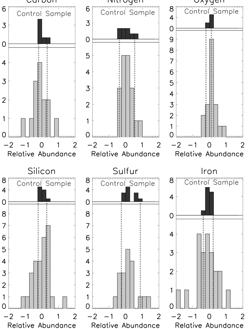
Figure 3: These are histograms of the relative abundances of carbon, nitrogen, oxygen, silicon, sulfur, and iron for the sample of high latitude B stars. The nearby Population I control sample is plotted at the top of each histogram for comparison. The dotted vertical lines are the minimum and maximum value in the nearby Population I control sample.

The elemental ratios and discussion of elemental abundances are based on the major ionization species, which is often the one with the most lines measured. Figure 3 shows the distribution of elemental abundances in the sample of study measured relative to the control sample.

4.7 Abundance Ratios

4.7.1 Selecting Referents

Abundance ratios are helpful for determining the pattern of enhancements and depletions in a stellar atmosphere. Of primary interest to this study are enhancements of carbon, nitrogen, oxygen, s-process, $\alpha$-process, and refractory elements which are used to distinguish between BHB, PAGB, PPN, and main sequence stars. In order for a ratio to effectively detect an enhancement, depletion, or lowered measured abundance of an element it must be compared to another element that is unaffected by the process for which one wishes to test.

An element which is unaffected by all of these processes would be the ideal universal referent. Pragmatism dictates that the referent selected must be measurable over the same range of atmospheric parameters as the element that is being tested for variation. However, it has proven difficult to identify one element with all these qualities so instead several different elements are used as referents, each with its own strengths and weaknesses.

Iron is often used as a referent. However, it can be affected by dust grain formation (especially in PAGB stars). Also, iron has few prominent lines in hotter stars making it difficult to measure its abundance, especially in stars with significant vsin(i). Table 5 demonstrates that minor species of iron tend to be more affected by small changes in the temperature and pressure structure of the stellar atmosphere. Additionally, iron’s high atomic weight gives it a smaller thermal velocity, which makes it more sensitive to changes in microturbulence.

Aluminum is a good referent because it remains untouched by most of the nuclear processes that affect the photospheric composition of stars through the PAGB and PPN phase. Also, Al III lines are prominent and easy to measure in hot B stars. However, aluminum is affected by the initial composition of the star (Edvardsson et al., 1993; Tomkin, Lambert, & Balachandran, 1985) and its measured abundance can be lowered by dust formation. The effect of initial composition is slight and will not hinder the ability to measure significant enhancements in other elements due to most nuclear processes. The influence of dust formation on the aluminum abundance can be more significant. However, aluminum is still a good referent as long as one keeps in mind that its abundance may be lowered in some stars which can be identified by other means.

Oxygen is a good referent to use with carbon and nitrogen to test for the presence of CNO processed material. It is affected less by that process than carbon or nitrogen and the oxygen abundance may be measured from many prominent O II lines over the entire range of stellar atmospheric parameters in B stars. However, one should be aware though that there are processes in later stages of stellar evolution that might enhance oxygen abundances (Imbriani et al., 2001).

Sulfur is the best element in this study to measure the lowering of abundances due to grain formation. However, it is an $\alpha$-process element which is also affected by initial composition. This effect may cancel out to first order if sulfur is used as a referent to measure the lowering of the abundance of another $\alpha$-process element, like silicon.

4.7.2 Ratios in the Program Stars

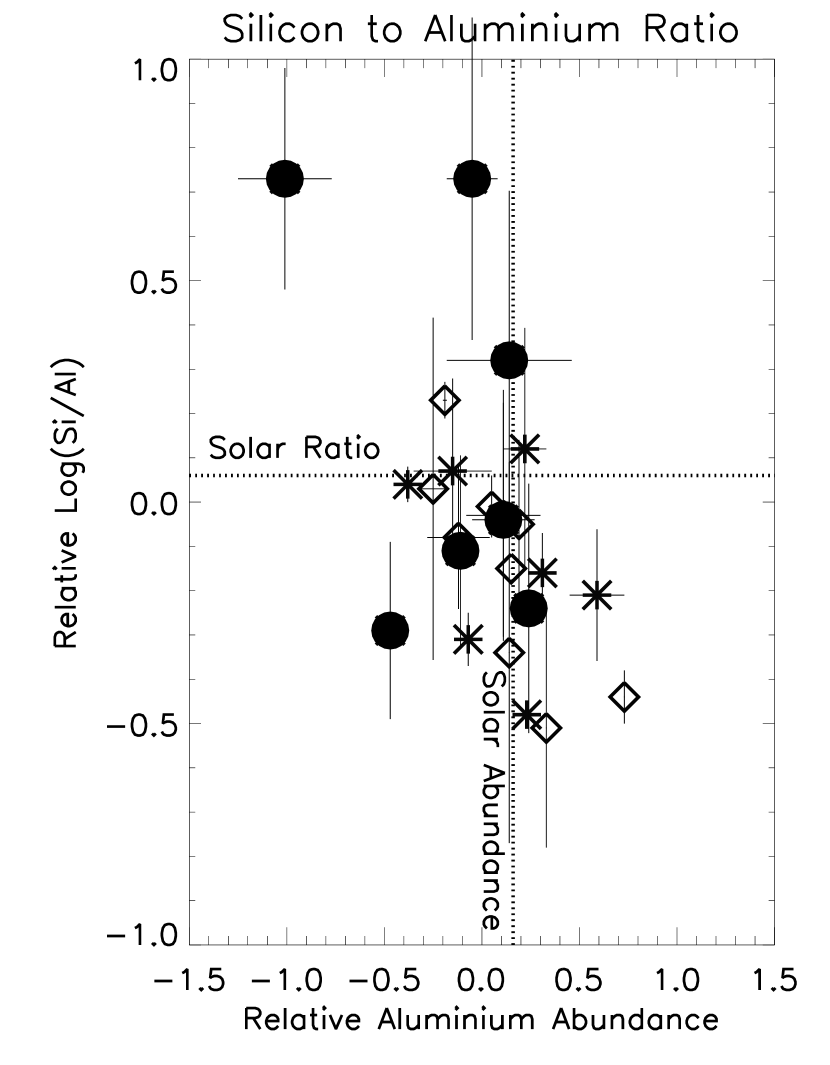
Figure 4: The diamonds are the nearby Population I control sample. The solid circles and *’s are the program stars which respectively have and do not have more than one abundance ratio which are more than two standard deviations from the mean of the control sample (see section 4.7.2).

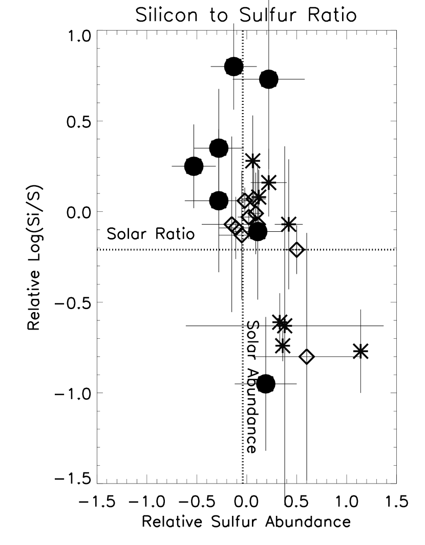
Figure 6: The diamonds are the nearby Population I control sample. The solid circles and *’s are the program stars which respectively have and do not have more than one abundance ratio which are more than two standard deviations from the mean of the control sample (see section 4.7.2).

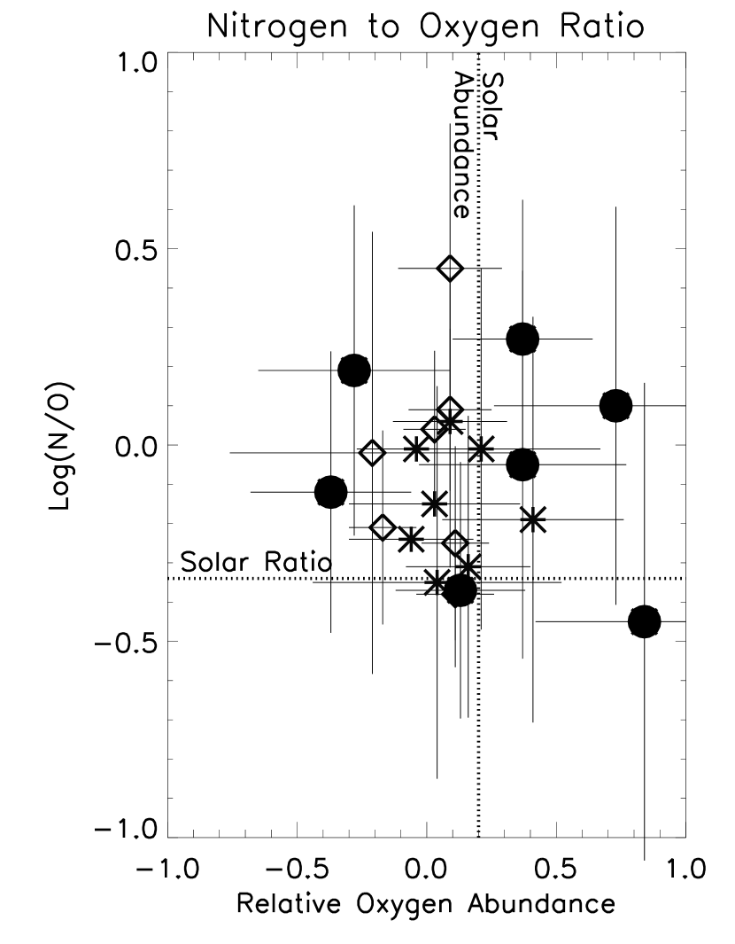
Figure 7: The diamonds are the nearby Population I control sample. The solid circles and *’s are the program stars which respectively have and do not have more than one abundance ratio which are more than two standard deviations from the mean of the control sample (see section 4.7.2).

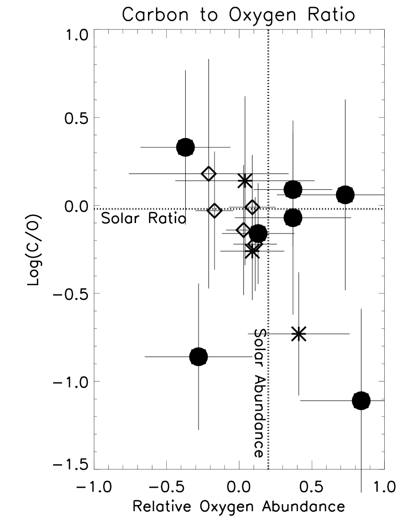
Figure 8: The diamonds are the nearby Population I control sample. The solid circles and *’s are the program stars which respectively have and do not have more than one abundance ratio which are more than two standard deviations from the mean of the control sample (see section 4.7.2).

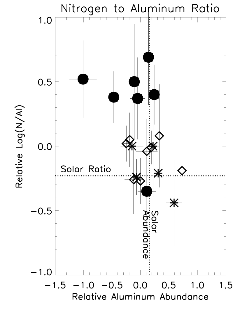
Figure 9: The diamonds are the nearby Population I control sample. The solid circles and *’s are the program stars which respectively have and do not have more than one abundance ratio which are more than two standard deviations from the mean of the control sample (see section 4.7.2).

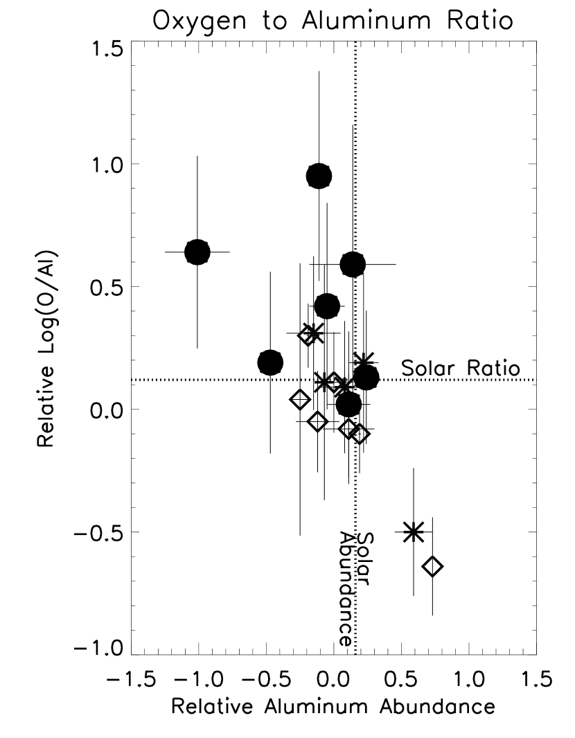
Figure 10: The diamonds are the nearby Population I control sample. The solid circles and *’s are the program stars which respectively have and do not have more than one abundance ratio which are more than two standard deviations from the mean of the control sample (see section 4.7.2).

The abundance ratios measured in the program stars and BHB and PAGB control samples are in Table 9. Three ratios, Si/Al (Figure 4), Mg/Fe (Figure 5), and Si/S (Figure 6), are used in this study to detect the influence of initial composition and dust formation on the measured abundances. Meanwhile, the N/O (Figure 7), C/O (Figure 8), N/Al (Figure 9), and O/Al (Figure 10) ratios are used to identify enhancements that could be due to mixing of processed material into a stellar atmosphere. These ratios must be interpreted keeping in mind that they involve species which are affected by the temperature and pressure structure of the atmosphere. Therefore, in some cases these ratios can be more sensitive to the assumptions made about the atmosphere than the composition.

For each abundance ratio the distribution of values in the nearby star control sample (plotted as open diamonds in Figures 4 through 10) is used to determine the usual distribution of values found among Population I B stars in the disk. Exceptional abundance ratios for program stars (more than two standard deviations from the mean of the control sample) are italicized and underlined in Table 9. Seven program stars (BD -15 115, HD 21305, HD 40276, HIP 41979, BD +36 2268, PB 166, and BD +33 2642) have more than one exceptional abundance ratio. HD 21305, HIP 41979, and PB 166 are probably BHB stars (see section 4.9) and BD +33 2642 has been classified as a proto-planetary nebula with abundances which have been affected by an initial metal poor halo composition and dust formation (Napiwotzki, Heber, & Koeppen, 1994; Napiwotzki, Herrmann, Heber, & Altmann, 2001)(see Appendix A). These stars which have abundance ratios that are persistently different from the nearby Population I control sample (plotted with solid circles in Figures 4 through 10) are the best candidates to be old low mass evolved stars. Eight more program stars (HD 21532, BD +61 996, HD 233622, HD 105183, HD 146813, HD 149363, HD 209684, and HD 218970) have one exceptional ratio each. The argument could be made to also classify these eight stars as low mass evolved stars based on their abundance ratios. However, their status is less certain.

4.8 Classification Based on Abundances

The results of the abundance analysis divide the sample of high galactic latitude B stars into three categories which are given in Table 9: disk, metal poor (MP), or old evolved star (OES). The results for the BHB and PAGB star control samples are also presented in Table 9 for comparison. Unfortunately it was not possible to obtain abundances for every element in each star so in some cases the picture presented by the relative abundances and ratios is incomplete. In those cases the uncertainty has been noted through a question mark (?) after the classification. The “Disk” category contains twenty two (22) stars which have abundances and ratios consistent with nearby Population I B stars. Presumably these stars are the best candidates for consideration as runaway stars ejected from the disk. The “old evolved star” category includes nine stars which have a pattern of enhancements and depletions of key elements which could be the result of advanced stellar evolution. Eight stars can only be characterized as “metal poor” (MP) with abundances which are uniformly lower than the control sample. Those stars could potentially turn out to be old evolved stars or stars which formed in situ in the galactic halo.

4.9 Metal Rich BHB Stars

Two stars in the sample (HIP 41979 and PB 166) have atmospheric parameters, abundance patterns, and projected rotational velocities which are consistent with hot horizontal branch stars. Each of these stars have CNO ratios consistent with post main sequence evolution and mixing as well as high iron abundances which are be indicative of a purely radiative BHB atmosphere affected by diffusion (Michaud, Vauclair, & Vauclair, 1983). Curiously, the magnesium abundance, which is unaffected by radiative diffusion (Behr, Cohen, McCarthy, & Djorgovski, 1999; Behr, Cohen, & McCarthy, 2000), is solar in these stars. This is surprising since metal rich populations should not produce BHB stars (Iben & Rood, 1970; Rood, 1973) and surveys of BHB stars in the solar neighborhood have not found any with abundances above 1/10 solar (Kinman, Suntzeff, & Kraft, 1994; Kinman et al., 2000). Therefore, these BHB stars are a significant find, especially since they are much nearer and brighter than the others discovered to date (Liebert, Saffer, & Green, 1994; Peterson, Terndrup, Sadler, & Walker, 2001; Peterson & Green, 2002).

HD 21305 has an abundance pattern and projected rotational velocity which are also consistent with a solar metallicity BHB star affected by diffusion. However, the atmospheric parameters of HD 21305 ($T_{eff}$ = 18500 K; log(g) = 4.0) are more consistent with a main sequence or PAGB star since its surface gravity is about 0.4 dex above the terminal age horizontal branch (TAHB). The analysis of this star’s kinematics in Paper II will be the decisive factor which will determine if it is the third metal rich BHB in the sample.

5 Other Data from Spectra

5.1 Strength of Helium Lines

The abundance of helium can be affected by stellar evolution. For example, some older evolved stars have helium abundances which are higher than those found in “normal” Population I B stars. On the other hand, radiative diffusion causes the the equivalent widths of He I lines in BHB stars to appear weaker than main sequence stars with solar abundances (Greenstein, Truran, & Cameron, 1967).

The neutral helium lines in the spectra of B stars can be heavily influenced by NLTE factors and multiple blended components which make it difficult to calculate absolute abundances. Relative helium abundances can be determined by comparing the equivalent widths of lines in two stars with the same atmospheric parameters. Figure 11 shows that almost all the high latitude B stars and the nearby Population I B stars fall on the same distribution as a function of effective temperature, indicating that they have similar helium abundances. There are a few stars with equivalent widths that are significantly larger or smaller than the control sample.

HIP 41979 (the high point at 18000 K) has consistently larger equivalent widths than the rest, indicating that it could possibly be helium enriched. BD +13 3224 (V625 Her) is also overabundant in helium (Jeffery, Woolf, & Pollacco, 2001). However, it has not been plotted in Figure 11 because its short pulsational period and rapidly changing photosphere conspired with the long exposure times in this study to render the spectrum recorded for it unmeasurable. Meanwhile, HD 21305, HD 105183, and PB 166 have equivalent widths which are consistently smaller than the control sample, indicating that they could possibly be BHB stars affected by diffusion.

In addition to having abnormal He I equivalent widths, HD 21305, HIP 41979, and PB 166 also have abundance patterns which suggest that they are metal rich BHB stars (see Section 4.9). It is unusual that HIP 41979 has larger than normal He I equivalent widths since BHB stars affected by diffusion should appear to be deficient in helium (leading to smaller than normal equivalent widths). Ramspeck, Heber, & Edelmann (2001) identified three BHB stars with a similar abundance patterns which also appear to have elevated helium abundances. It appears that HIP 41979 also fits into this group of BHB stars which without clear explanation defy conventional wisdom concerning the mechanics of radiative diffusion in BHB atmospheres.

5.2 Emission Features

Exposures were taken in sets so that emission features, which appear in every exposure, could be distinguished from cosmic ray hits. Great care was taken during processing to identify any emission features in the observed spectra. Spectral emission features were only found in two of the sample stars (BD +33 2642 and Feige 23).

BD +33 2642 is a previously identified halo proto-planetary nebula (PPN) (Napiwotzki, 1993; Napiwotzki, Heber, & Koeppen, 1994). It has an unusual spectrum composed of a blend between classic nebular emission lines and a stellar photospheric absorption spectrum, which allows a unique opportunity to analyze the abundances of both the nebula and the central star. This analysis and a more extensive discussion of this object are in presented in Appendix A.

Feige 23 has a normal spectrum with very narrow sodium D emission lines (Figure 12). This emission, combined with inconsistencies in the (B-V) colors measured for this star (Klemola, 1962; Blanco, Demers, & Douglass, 1970; Kilkenny, 1995; Turon et al., 1997) are probably indicative of some kind of dust shell or other aggregation of circumstellar material.

5.2.1 Be Stars

Curiously, there are no stars in this sample which exhibit the classic emission features used to identify Be stars. The frequency of Be stars among nearby stars (Zorec & Briot, 1997) leads to the expectation that a sample of this size and distribution of spectral types should have about ten Be stars. It is important to note that the number of Be stars in a sample will almost always be underestimated because Be stars do not always exhibit emission features. Also, only the runaway Population I B stars in the sample are potentially drawn from the same population as the nearby stars surveyed by Zorec & Briot (1997). Even taking these factors into account it seems unlikely that the sample would have no identifiable Be stars in it unless somehow the ejection mechanisms for runaway B stars select against stars exhibiting the Be phenomenon.

Be stars tend to rotate faster than the general population (Slettebak, 1982) and are also thought to be created through interaction with a close companion in a binary system (for a review and references see Porter & Rivinius (2003a)). Therefore, a population with few fast rotators and no binary companions might have few if any Be stars. Runaway B stars are far less likely to have binary companions than B stars in the disk field population (Gies & Bolton, 1986). However, it will be shown in Paper II that the average vsin(i) of runaway B stars is faster than the average vsin(i) of nearby disk B stars. Is it possible that the lack of binary companions by itself could be responsible for the absence of Be stars from our sample? We do not know. However, further study of high latitude B stars may yield more information about the origin of the Be phenomenon.

6 Conclusions

6.1 Preliminary Classification of the Sample

Detailed photospheric elemental abundance analysis of forty program stars has revealed that while twenty two stars in the sample have abundances which appear to be indistinguishable from nearby Population I B stars, nine others have abundance patterns which strongly indicate that they are old evolved stars, eight have abundance patterns which are metal poor, and one (HD 1112) has an abundance pattern which we are unable to classify. We also found that AG +03 2773 is probably an rapidly rotating F dwarf which has been misclassified as a B star. The lines in the spectrum of AG +03 2773 are broad and numerous so that they effectively obliterate the continuum at most wavelengths and make it difficult to perform an abundance analysis.

In addition to the abundance data, we found that seven stars in our sample have spectral peculiarities which are best interpreted by phenomenon which are not expected in runaway Population I B stars: He I equivalent widths outside the range in ”normal” B stars of a given temperature, and/or odd spectral emission features. Five of these stars also have abundance patterns presented here which verify that they are probably old evolved stars and one of the remaining two (BD +13 3224) is a previously identified pulsating helium dwarf.

Table 11 gives a preliminary classification of each star. The sample is broken into four categories:

• Population I runaway (Pop I; 21 stars),

• Old evolved BHB or PAGB star (OES; 10 stars),

• F dwarf (1 star),

• or unknown (17 stars).

The category “unknown” covers stars with insufficient or conflicting information which preclude their placement in one of the other categories. Therefore at this stage, “unknown” includes any B stars formed in situ in the halo since we require an analysis of a star’s kinematics and past trajectory to make that classification with certainty. These classifications were made conservatively in order to minimize the number of stars that might migrate from the Population I to the old evolved star category when the results from the kinematic data are considered in Paper II.

6.2 Comparison with Other Work

A number of the stars in our sample have been categorized individually or in small groups by other studies. In most cases those classifications agree with the classifications made here. This includes: BD -15 115 (Ramspeck, Heber, & Moehler, 2001; Magee et al., 2001), BD +38 2182 (Conlon, Brown, Dufton, & Keenan, 1989), HD 100340 (Ryans et al., 1999), HD 105183 (Dufton et al., 1993), Feige 40, PB 166 (de Boer, Richtler, & Heber, 1988), Feige 84 (Lynn et al., 2004; Saffer et al., 1997), HD 123884 (Bidelman, 1988), HD 137569 (Danziger & Jura, 1970), HD 138503 (Martin, 2003), BD +33 2642 (See Appendix I), and BD +13 3224 (Jeffery, Woolf, & Pollacco, 2001; Jeffery & Hill, 1986).

Two of the stars in this study have received classifications which potentially conflict with the results from other assorted studies. Conlon et al. (1992) classified HD 121968 as a normal Population I B star. We have no spectrum to measure the abundances for this star. Indications are that it is probably a runaway. However, we are reserving judgment until after we have analyzed its kinematics so for the moment it remains classified “unknown.”

Zboril & North (2000) classified HD 149363 as a slightly helium rich evolved star with carbon enhancement but normal nitrogen and oxygen abundances. However, we classify HD 149363 as a Population I runaway because unlike Zboril & North (2000) we observe no abnormality in the strength of the helium lines and measure carbon, nitrogen, and oxygen abundances which do not differ significantly from stars in the nearby Population I control sample. Zboril & North (2000) used nearly the same temperature and gravity to analyze this star. Therefore, the difference between our results is probably due to the microturbulence and/or the atomic transitions measured. Zboril & North (2000) adopted a microturbulence value of 6km/s while this work measured a microturbulent velocity of 20 km/s. If the microturbulence is reduced to 6 km/s in our analysis then the abundances of carbon, nitrogen, silicon and sulfur rise by 0.3 dex, aluminum abundance rises by 0.4 dex, and oxygen abundance rises by 0.5 dex. This does not completely match the pattern of abundances which they reported. In addition to the difference in microturbulence, Zboril & North (2000) use of the C II 4267 Å doublet alone to measure carbon abundance. It is well established that this feature is an unreliable measure of absolute carbon abundance due to very strong NLTE effects (Sigut, 1996; Kane, McKeith, & Dufton, 1980). Zboril & North (2000) argue that these effects should lead to a systematic underestimate of carbon abundance rather than an over abundance. However, with the difference in microturbulence included, the behavior of this transition may account for the difference between our analyses.

Fifteen stars in our sample were also cited by Conlon et al. (1992) as stars with full space velocities which imply that they were ejected from the galactic disk. We have classified all these stars, with the exception of BD +36 2268, as either Population I runaways (nine stars) or stars which we are reserving judgment about until we have analyzed their space velocities (five stars). BD +36 2268 may well have a space velocity consistent with ejection from the galactic disk but it also has several abnormal abundance ratios (see Table 9) which imply that is is an old evolved star. In this case, the abundance analysis should be given precedence because kinematics alone are unable to determine which stars are old evolved post-main sequence objects.

Behr (2003) classified 21 stars in this study according to their position relative to evolutionary tracks on an $T_{eff}$ versus log(g) plot. The effective temperatures and surface gravities derived by Behr for these stars closely match the values which we have adopted in this study. Behr (2003) also measured the LTE abundances of iron and magnesium relative the solar values. All but one of the iron and magnesium abundances measured in this study are consistent with Behr’s values within the quoted errors. (The discrepancy in the iron abundance of BD +30 2355 is discussed below.) There are also no conflicts between our classifications and Behr’s for 16 of the 21 common stars. The difference in classification for the remaining five stars mostly arises from the consideration of additional information which Behr (2003) did not incorporate into their study.

HD 1112, HD 233622, HD 105183, and BD +36 2268 (classified ”main sequence” by Behr (2003)) are classified as OES or “unknown” here because they have abundance patterns which are not consistent with the nearby Population I star control sample. This study analyzes the abundances of several light elements, including carbon, nitrogen, and oxygen, which are affected by stellar evolution while Behr (2003) only considered the abundances of iron and magnesium in the context of matching stars to evolutionary tracks. In addition to having a pattern of enhancements and depletions of specific elements which is indicative of post-main sequence evolution, HD 105183 also has weaker than expected helium lines, which is more typical of an OES.

BD +30 2355 was classified by Behr (2003) as a “possible” BHB star. Whereas, we classify it as Pop I. In the discussion of their results Behr (2003) expressed some reservations about their own classification for this star since its vsin(i) is rather large (100 km/s) for a BHB star. While Behr measured the [Fe/H] of BD +30 2355 to be $-2.70\pm 35$ from an unspecified number of lines we found that its iron abundance was only $-0.22\pm.38$ dex relative to the Population I control sample (measured from two lines). There is a difference in the microturbulence values which each of us adopt (2km/s for Behr and 5km/s for us). However, lowering the microturbulence to 2 km/s in our analysis raises the iron abundance by almost one dex. In final analysis, the source of the disagreement between this study and Behr (2003) is unclear. Since we have measured a disk-like metallicity and no other spectral peculiarities for BD +30 2355, we have given it a preliminary classification of Pop I, pending verification by examination of its space velocity in Paper II.

6.3 Other Results

Among the stars in the sample with old evolved star abundances, there are as many as three solar metallicity BHB stars. These metal rich BHB stars are much closer and brighter than the others discovered to date. We are reasonably certain that HIP 41979 and PB 166 are correctly identified as metal rich BHB stars. However, conflicting information about HD 21305 means that its classification depends on the kinematic data to be presented in Paper II.

It is surprising to find that there are no active classical Be stars in this sample. While there is a slight chance that small number statistics may be responsible, this seems unlikely. The only difference we can find between runaway B stars and Be stars (other than the defining emission features) is the low incidence of binary companions among runaways. Further study is required to tell whether or not this is the factor responsible for the missing Be stars in our sample.

In Paper II we will present the kinematic data for the stars in the sample. We will use this data and simulations to show that the space velocities of runaways retain a distinct kinematic signature which can be used to separate them from halo stars. We will also calculate and compare the flight times and main sequence lifetimes of the stars in the sample in order to determine which of them could have originated in the disk. That data will be combined with the data from this paper to classify each star as a Population I runaway, an old evolved star, or a star formed in situ in the halo. With a sample of Population I runaways in hand we will analyze their distribution of ejection velocities and projected rotational velocities in order to gain insight into the mechanisms which ejected them from the disk. Additionally, we will also analyze the vsin(i) of PAGB stars and the kinematics and origins of the BHB stars identified in the sample.

7 Acknowledgments

I want to thank my mentor and friend R. Earle Luck for his tireless support of my research and his continued thoughtful questioning and input. Apparently an advisor’s work is never done. I also want to thank the rest of my dissertation committee, Heather Morrison, J. Chris Mihos, and Robert Dunbar for their different perspectives which enriched this final product. I want to thank Kris Davidson and Roberta Humphreys for providing me with the time, environment, and encouragement to finish distilling this research into a publishable form. This work was supported in part by the Jason J. Nassau Scholarship Fund and the Townsend Fund through the generous continued support of the Ford, Nassau, and Townsend families.

Appendix A Appendix A: Proto-planetary Nebula BD +33 2642

BD +33 2642 is a known halo proto-planetary nebula (PPN) (Napiwotzki, 1993; Napiwotzki, Heber, & Koeppen, 1994) which has a spectrum with both classic nebular emission lines and a stellar photospheric absorption lines. This gives the unique opportunity to analyze both the nebula and the central star. Both the nebula and the central star are thought to be significantly iron deficient with enhancements of carbon, nitrogen, oxygen, and $\alpha$-process elements (Napiwotzki, Heber, & Koeppen, 1994; Napiwotzki, Herrmann, Heber, & Altmann, 2001). The abundances derived for the central star by this study and by Napiwotzki, Heber, & Koeppen (1994) for the central star and nebula are listed in Table 12.

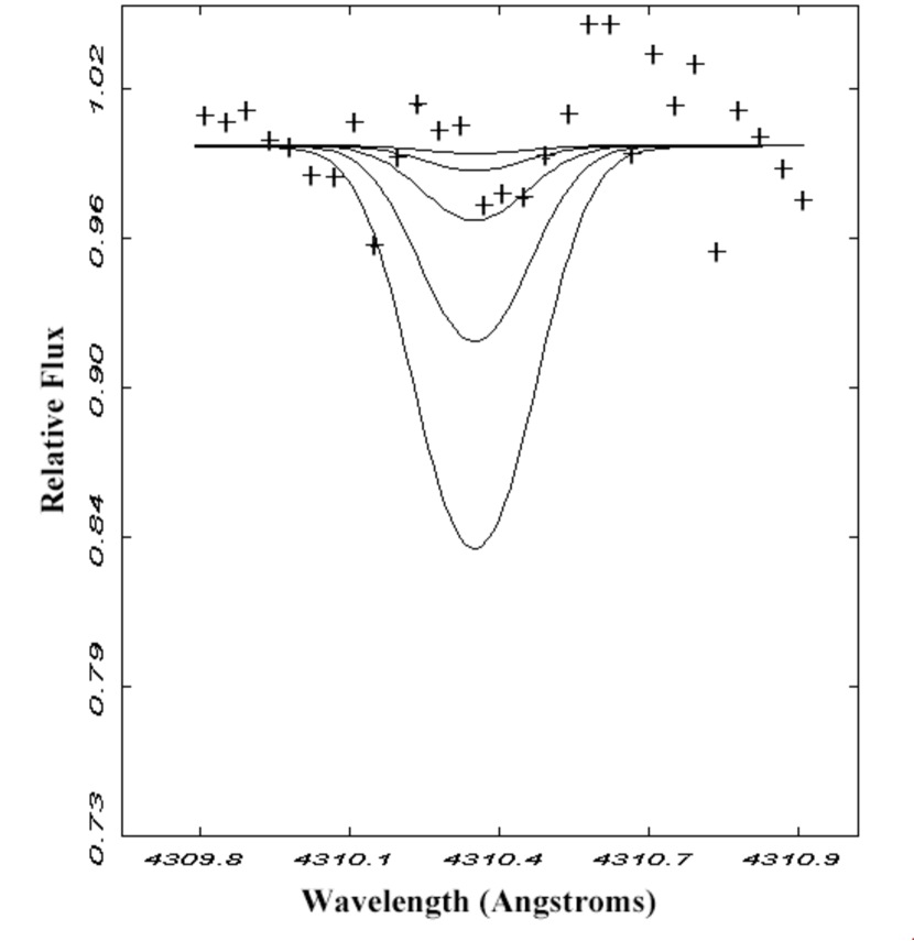
Figure 13: Fitting the Fe III 4310 line. The profiles from deepest to shallowest are: $log(\epsilon_{Fe})$= 7.50, 7.00, 6.50, 6.00, 5.50. The $log(\epsilon_{Fe})$= 6.5 profile appears to be the upper limit on the iron abundance.

Napiwotzki, Herrmann, Heber, & Altmann (2001) reassessed the iron abundance of the central star using a ultraviolet spectra from the HST-STIS spectrograph and found a slightly higher abundance of -1.5 dex relative to solar. A higher iron abundance is not ruled out by the observed nebular lines since they can also be reproduced from model with [Z/H] = -1.3 (Napiwotzki, Heber, & Koeppen, 1994). The data at hand can be used to set an upper limit on the iron abundance using the Fe III 4310 line. Figure 13 shows that the iron abundance can be no higher than about 6.50 dex ([Fe/H]=-1.0).

Both the carbon (from C II) and silicon (from Si III) abundances derived by this study are higher than those reported by Napiwotzki, Heber, & Koeppen (1994). However the abundance measured from Si III is more sensitive to the parameters adopted for the atmosphere. Table 13 compares the abundances derived from the equivalent widths in this study using the atmospheric parameters adopted for BD +33 2642 by Napiwotzki, Heber, & Koeppen (1994) and Fitzpatrick & Massa (1999). The abundances derived from C II, N II, and Al III are fairly insensitive to the choice of model parameters while abundances derived from O II, Si III, S III, and Ar II can be significantly affected. When the model parameters of Napiwotzki, Heber, & Koeppen (1994) are used, the silicon abundance as derived from Si III is in excellent agreement with the value which they published. However, the carbon abundance from C II remains higher.

The difference in carbon abundance is better explained by differences in atomic data. Napiwotzki, Heber, & Koeppen (1994) attempted to use the C II $4267\mbox{\AA}$ feature as one of four lines to measure the carbon abundance. This feature cannot be used to reliably measure LTE carbon abundance (Kane, McKeith, & Dufton, 1980). Two of the other three features (C II $6578\mbox{\AA}$ and C II $6583\mbox{\AA}$) used by Napiwotzki, Heber, & Koeppen (1994) are also used by this study. However, they use gf values which are significantly larger (Table 8). Therefore the difference in the carbon abundance is a result of the line choice and atomic data.

The differences in the carbon and silicon abundance have an impact on the interpretation of BD +33 2642. The higher carbon abundance translates into a significant carbon enhancement relative to nitrogen and oxygen which requires a reassessment of the nuclear processing and mixing that may have occurred in the star.

Likewise a higher silicon abundance may require a change in the grain formation scenario which is invoked to explain the lowered iron and aluminum abundances in the central star. Because different processes affect grain formation for different elements, it is not expected that silicon will be lowered to the same degree as iron or aluminum. However, there is no evidence from the silicon abundance that grain formation occurred since the silicon abundance is not lowered significantly with respect to the non-refractory elements argon and sulfur. It is not clear if any grain formation scenario could lower the abundance of aluminum and iron and leave silicon untouched.

Napiwotzki, Herrmann, Heber, & Altmann (2001) also reported evidence for long-term (on the order of many years) variability in the radial velocity of the central star, which they cite as evidence of an unseen companion. However, the radial velocity data in this study does not conclusively show any variability. Table 14 shows that there is a $4.8\pm 10.6$ km/s difference in the radial velocity measured for BD +33 2642 in July 1998 and March 2001. The heliocentric radial velocity measured in July 1998 ($-92.3\pm 2.1$ km/s) is consistent with the systemic velocity adopted by Napiwotzki, Herrmann, Heber, & Altmann (2001) (-94 km/s). There is enough uncertainty in this measurement that a binary companion cannot be completely ruled out however this data does appear to conflict with the the model presented by Napiwotzki, Herrmann, Heber, & Altmann (2001).

Figure 2: A plot of the logarithm of the vsin(i) measured in this study versus the value given in other sources. The triangles are the nearby B star control sample compared with vsin(i) values from the Yale Bright Star Catalog. The diamonds are stars from the sample of study compared with values measured by Behr (2003). The vertical lines attached to the diamonds represent Behr’s quoted errors.

Figure 5: The diamonds are the nearby Population I control sample. The solid circles and *’s are the program stars which respectively have and do not have more than one abundance ratio which are more than two standard deviations from the mean of the control sample (see section 4.7.2).

Figure 11: The equivalent widths of four He I lines versus effective temperature. The equivalent widths of the nearby Population I control sample are the black diamonds. The + s are the program stars.

Figure 12: The sodium D lines in emission in the spectrum of Feige 23.

Table 1: Sample of Study

Hipparcos	FB	Common	RA	Dec	Spectral		Z	Gal Lat	Parallax
Number	Number	Designation	(J2000)	(J2000)	Class	V mag	(kpc)	(deg)	(mas)
1214	5	HD 1112	00 15 27.28	-03 39 15.1	B9	9.110	0.43	-44.33	$1.67\pm 1.22$
1511	$\cdots$	$\cdots$	00 18 49.79	+30 23 33.7	B8	11.610	1.22	-31.95	$0.37\pm 2.82$
3013	7	BD -15 115	00 38 20.26	-14 59 54.2	B2	10.879	4.42	-77.49	$1.52\pm 1.80$
6419	16	HD 8323	01 22 24.88	-07 17 13.0	A0	9.610	0.59	-68.84	$1.19\pm 1.31$
6727	17	BD -7 230	01 26 38.44	-06 20 18.7	$\cdots$	11.130	1.54	-67.59	$4.64\pm 2.22$
11809	22	Feige 23	02 32 17.19	+02 59 52.7	B6V	11.080	1.94	-51.28	$1.68\pm 4.25$
11844	23	HD 15910	02 32 54.48	-20 20 12.0	B9IV/V	10.105	1.05	-65.85	$0.81\pm 1.64$
12320	25	$\cdots$	02 38 37.78	+05 28 11.3	B7	12.040	2.52	-48.36	$3.92\pm 5.81$
15967	$\cdots$	HD 21305	03 25 35.93	-20 20 03.6	B4III	10.345	3.15	-54.21	$-1.44\pm 2.07$
16130	30	HD 21532	03 27 46.36	-21 23 50.7	B7V	9.880	0.97	-54.05	$-0.89\pm 1.48$
28132	$\cdots$	HD 40276	05 56 47.03	-22 17 55.0	B3II/III	9.700	1.27	-21.56	$0.05\pm 1.44$
37903	$\cdots$	BD +61 996	07 46 02.54	+61 21 47.1	B2	9.800	1.38	+30.06	$1.47\pm 1.29$
41979	$\cdots$	$\cdots$	08 33 20.33	+20 24 24.9	B2V	11.451	3.05	+31.18	$1.02\pm 2.79$
45904	54	HD 233622	09 21 33.60	+50 05 56.4	B5	9.964	1.19	+44.23	$-1.23\pm 1.57$
48394	$\cdots$	HD 237844	09 51 57.97	+55 43 32.4	B3	10.190	1.67	+47.06	$-1.66\pm 1.54$
50750	63	BD +16 2114	10 21 47.06	+15 32 03.6	$\cdots$	9.870	0.72	+53.44	$1.26\pm 1.51$
52906	66	BD +38 2182	10 49 12.92	+38 00 14.8	B2	11.230	4.71	+62.22	$-1.10\pm 2.01$
55461	72	Feige 40	11 21 29.35	+11 19 17.1	B6	11.132	2.28	+63.62	$0.73\pm 2.16$
56322	76	HD 100340	11 32 49.94	+05 16 36.1	B9	10.130	0.85	+61.23	$0.70\pm 1.45$
58046	79	HD 103376	11 54 17.17	+18 37 22.7	B5	10.188	1.83	+74.33	$-1.22\pm 9.19$
59067	83	HD 105183	12 6 47.24	+11 40 12.7	B5	11.100	2.73	+71.31	$0.87\pm 2.39$
59955	92	HD 106929	12 17 49.97	+10 07 12.0	B9	9.800	0.79	+71.24	$0.72\pm 1.41$
60578	96	BD +49 2137	12 25 00.40	+49 08 30.6	B7V	10.640	1.60	+67.40	$1.52\pm 1.76$
60615	97	BD +36 2268	12 25 23.45	+35 58 33.5	B3	10.422	2.50	+79.55	$0.17\pm 1.42$
61800	104	HD 110166	12 39 56.99	+36 59 53.7	B8V	8.760	0.59	+79.84	$2.18\pm 1.16$
63591	119	BD +30 2355	13 01 52.97	+29 34 57.2	B9	10.645	1.23	+41.39	$-4.22\pm 1.73$
65388	$\cdots$	PB 166	13 24 00.75	+49 22 32.2	B2	12.450	8.58	+66.88	$4.07\pm 2.92$
66291	135	Feige 84	13 35 11.99	+13 27 44.2	B3p	11.844	4.67	+72.93	$3.49\pm 2.81$
68297	141	HD 121968	13 58 51.17	-02 54 52.5	B5	10.310	1.65	+55.84	$-0.87\pm 1.68$
69247	$\cdots$	HD 123884	14 10 33.78	-17 59 27.3	B8/B9Iap..	9.324	8.33	+40.97	$1.77\pm 1.40$
70275	146	HD 125924	14 22 42.99	-08 14 53.5	B2IV	9.680	2.67	+48.28	$-1.88\pm 1.40$
71667	153	BD +20 3004	14 39 31.26	+19 25 43.5	B8	10.150	1.03	+64.07	$-0.75\pm 1.44$
75577	158	HD 137569	15 26 20.81	+14 41 36.4	B5III	7.950	0.84	+51.93	$-0.01\pm 0.85$
76161	$\cdots$	HD 138503	15 33 18.91	-25 01 37.0	B2/B3IV:n.	9.180	1.20	+24.87	$-0.71\pm 1.30$
77131	$\cdots$	HD 140543	15 44 56.66	-21 48 53.9	B1Iabn	8.885	4.82	+25.54	$1.36\pm 1.52$
77716	162	BD +33 2642	15 51 59.90	+32 56 54.3	B2	10.835	3.44	+50.79	$-0.46\pm 1.50$
79649	164	HD 146813	16 15 14.80	+55 47 58.4	B8	9.080	0.50	+43.81	$2.41\pm 0.78$
81153	$\cdots$	HD 149363	16 34 28.28	-06 08 10.2	B0.5III	7.772	1.69	+26.69	$0.16\pm 1.12$
82236	168	BD +13 3224	16 48 04.70	+13 15 42.4	B1	10.546	3.08	+33.28	$0.90\pm 1.77$
96130	$\cdots$	HD 183899	19 32 45.18	-26 09 46.6	B1/B2II	9.795	3.77	-20.14	$3.99\pm 1.86$
98136	$\cdots$	HD 188618	19 56 40.48	-17 55 17.0	B2II	9.381	2.59	-22.22	$-2.10\pm 1.50$
104931	$\cdots$	AG +03 2773	21 15 18.47	+03 25 09.5	B5	10.800	1.24	-29.64	$-0.23\pm 2.05$
107027	$\cdots$	HD 206144	21 40 33.38	-17 36 00.5	B2IIn…	9.383	4.86	-45.12	$-0.94\pm 1.33$
109051	$\cdots$	HD 209684	22 05 31.16	-13 46 12.8	B2/B3III	9.841	4.24	-49.13	$2.27\pm 1.49$
111396	180	HD 213781	22 34 04.58	-12 09 29.6	B8/B9III	9.040	0.77	-54.53	$0.51\pm 1.61$
112790	181	HD 216135	22 50 28.24	-13 18 44.2	B5V	10.114	1.56	-58.56	$2.83\pm 1.80$
114569	183	HD 218970	23 12 30.60	-21 06 43.7	B2/B3IV/V	9.740	1.71	-66.68	$1.86\pm 1.59$
115729	187	HD 220787	23 26 45.49	-11 01 57.3	B3III	8.310	1.64	-64.40	$1.75\pm 1.13$
116560	$\cdots$	HD 222040	23 37 17.68	-20 55 54.9	B9IV	10.882	1.57	-72.00	$-6.62\pm 2.31$

Table 2: Abundance Control Samples

	RA	Dec	Spectral		V sin(i)
Star	(J2000)	(J2000)	Class	V mag	(km/s)
Population I B Star Control Sample
Gam Peg	00 13 14	+15 11 01	B2 IV	2.83	3
HR 1220	03 57 51	+40 00 37	B0.5 V	2.90	153
HR 1397	04 26 21	+08 35 25	B6 IV	6.07	25
Bet Ori	05 14 32	-08 12 06	B8Iab	0.12	33
Gam Ori	05 25 08	+06 20 59	B2 III	1.64	59
HR 2010	05 49 33	+12 39 05	B9 IV	4.88	22
HR 2928	07 36 41	-19 42 08	B2 II	5.69	38
HR 4187	10 40 35	+57 27 44	A0 V	5.79	27
HR 6165	16 35 53	-28 12 58	B0 V	2.81	24
Nu Cap	20 20 40	-12 45 33	B9 IV	4.75	17
HR 8404	22 03 19	+11 23 12	B9.5 V	5.82	2
HR 8768	23 02 45	+44 03 32	B2 V	6.41	25
BHB Control Sample
HD 60778	07 36 12	-00 08 16	A1 V	9.12	10
HD 74721	08 45 59	+13 15 49	A0 V	8.71	3
PAGB Control Sample
HD 18100	02 53 41	-26 09 20	B5II/III	8.44	220
HD 44179	06 19 58	-10 38 15	B8 V	9.02	20
HD 105262	12 07 11	+12 59 08	B9	7.09	6
HD 119608	13 44 31	-17 56 13	B1Ib	7.50	50

Table 3: Results From Temperature & Gravity Relations

	Extinction		Johnson	Strömgren	Geneva		Balmer
Star	E(B-V)	Ref	$T_{eff}$	$T_{eff}$	$T_{eff}$	log(g)	log(g)
Program Stars
HD 1112	0.038	b	5703		$11455\pm 51$	$4.15\pm 0.09$	4.00
HIP 1511	0.065	a	7600	9090			3.00
BD -15 115	0.018	a	20322	19427	$19758\pm 198$	$3.94\pm 0.17$	4.00
HD 8323	0.043	a	12906		$13568\pm 80$	$4.05\pm 0.13$
BD -07 230	0.036	a	9876				3.75
Feige 23	0.028	a	5728	13265			4.25
HD 15910	0.023	a	10827	10984	$11205\pm 69$	$4.14\pm 0.08$	4.00
HIP 12320	0.086	a	13056	13382			4.00
HD 21305	0.010	c	15750	18042	$18574\pm 200$	$4.13\pm 0.15$	4.00
HD 21532	0.032	b	11858	13864	$13654\pm 69$	$4.27\pm 0.12$	4.50
HD 40276	0.043	a	19384		$16948\pm 140$	$4.00\pm 0.15$	3.50
BD +61 996	0.047	a	13808				3.00
HIP 41979	0.034	a	20983				4.50
HD 233622	0.016	a	21355	21074	$21321\pm 208$	$3.54\pm 0.21$	3.50
HD 237844	0.008	a	16606	20021			3.75
BD +16 2114	0.046	a	17935		$17171\pm 175$	$4.39\pm 0.14$
BD +38 2182	0.018	a	20322	18820			3.75
Feige 40	0.042	a	17560	15547			4.50
HD 100340	0.027	a	29387	24515	$26030\pm 364$	$4.17\pm 0.22$	4.25
HD 103376	0.010	d	14400	13357			4.25
HD 105183	0.038	a	14277	15145	$14971\pm 99$	$3.89\pm 0.15$	3.75
HD 106929	0.021	a	13865	13773	$13568\pm 92$	$4.42\pm 0.11$	4.00
BD +49 2137	0.013	a	14587	15155	$15413\pm 114$	$4.02\pm 0.14$
BD +36 2268	0.011	a	46451	19167			4.00
HD 110166	0.012	a	16688		$12552\pm 62$	$3.34\pm 0.16$	3.50
BD +30 2355	0.027	a	11533	9963			3.25
PB 166	0.011	a	36389	18954			4.75
Feige 84	0.020	c	18327	17478			4.25
HD 121968	0.066	a	24289	22465	$23756\pm 250$	$4.04\pm 0.19$
HD 123884	0.086	a	9735	11637	$11261\pm 259$	$2.61\pm 0.39$	LOW
HD 125924	0.048	a	23119	21839	$22997\pm 263$	$4.13\pm 0.19$
BD +20 3004	0.027	a	15531	13901
HD 137569	0.040	c	12292	12834	$12371\pm 123$	$2.89\pm 0.20$	LOW
HD 138503	0.227	a	26596	22060
HD 140543	0.270	c	36788	32042	$32095\pm 569$	$3.86\pm 0.25$	3.75
BD +33 2642	0.012	e	16688	21137	$21472\pm 199$	$3.38\pm 0.22$	3.00
HD 146813	0.009	a	23279	21225	$20848\pm 215$	$3.87\pm 0.18$	4.00
HD 149363	0.280	f	14647	29423	$30020\pm 773$	$4.05\pm 0.45$	3.25
BD +13 3224	0.058	a	17201	29867	$28088\pm 1118$	$4.12\pm 0.67$
HD 183899	0.180	d	27243		$23141\pm 239$	$3.63\pm 0.21$	4.25
HD 188618	0.254	a	11943	23678	$23235\pm 241$	$3.61\pm 0.22$	3.75
AG +03 2773	0.068	a	5691				3.75
HD 206144	0.078	b	17323	21762	$21968\pm 236$	$3.65\pm 0.21$	LOW
HD 209684	0.038	b	23093	20865	$20995\pm 256$	$4.14\pm 0.17$	4.25
HD 213781	0.060	f	16524	13946	$13857\pm 69$	$3.87\pm 0.14$	3.75
HD 216135	0.046	a	17027	15555	$15311\pm 108$	$4.15\pm 0.14$	4.00
HD 218970	0.027	a	20200	18677	$17862\pm 171$	$4.20\pm 0.15$	4.25
HD 220787	0.030	c	19384	17353	$17815\pm 178$	$3.92\pm 0.16$	3.75
HD 222040	0.026	a	8514		$8335\pm 70$	$3.10\pm 0.10$	3.25
Nearby Population I B Stars
Gam Peg	0.010	g	29647	20896	$21731\pm 222$	$3.80\pm 0.20$	4.00
HR 1220	0.090	g	27243	28215	$28825\pm 443$	$3.70\pm 0.24$	4.00
HR 1397	0.149	h	11414	14777	$14219\pm 80$	$3.98\pm 0.14$	3.75
Bet Ori	0.113	i	16747	17873	$18015\pm 163$	$3.43\pm 0.20$	LOW
Gam Ori	0.020	g		21697	$21760\pm 248$	$3.96\pm 0.18$	4.00
HR 2010	0.000	j	10723	10619	$10797\pm 134$	$4.20\pm 0.11$	4.00
HR 2928	0.058	h	24847	23056	$23803\pm 252$	$4.00\pm 0.19$	4.00
HR 4187	-0.001	k	9213	10003	$10357\pm 139$	$4.09\pm 0.10$	3.75
HR 6165	0.099	l	89160	32466	$30682\pm 1412$	$3.78\pm 0.68$	4.50
Nu Cap	0.000	j	9934	9714	$10193\pm 134$	$3.93\pm 0.10$	3.75
HR 8404	0.014	k	11206	10275	$10364\pm 124$	$3.56\pm 0.11$	3.50
HR 8768	0.230	g	21913	17620	$17704\pm 171$	$3.83\pm 0.17$	4.00
BHB Stars
HD 60778	0.020	m	8451	8956			3.25
HD 74721	0.000	n	9011	8991	$8707\pm 80$	$3.47\pm 0.10$	3.25
PAGB Stars
HD 18100	0.050	o	36000	24968	$26979\pm 1536$	$4.20\pm.89$	4.00
HD 44179	0.406	m	9084	8537	$8232\pm 112$	$2.67\pm 0.06$	LOW
HD 105262	-0.046	p	8819	9240			LOW
HD 119608	0.160	o	23441	27066	$26413\pm 891$	$4.09\pm 0.57$	3.50

Table 4: Stellar Parameters Used in the Analysis

	$T_{eff}$	Log(g)	Microturb ($\xi_{t}$)		Vsin(i)
Star	(K)	(dex)	(km/s)	Species	(km/s)
Program Stars
HD 1112	11500	4.00	10	Fe II	130
HIP 1511	9000	3.00	2	Fe II, Cr II	20
BD -15 115	19750	4.00	8	Si III	10
BD -07 230	10000	3.00	2	Fe II, Cr II, Ti II	6
Feige 23	13250	4.25	5	borrowed	240
HD 15910	11250	4.00	5	Fe II	130
HIP 12320	13500	4.00	5	borrowed	225
HD 21305	18500	4.00	9	Si III	15
HD 21532	13500	4.25	5	Fe II	60
HD 40276	17000	3.50	6	Si III, O II, N II	100
BD +61 996	18000	3.00	17	Si III, O II, N II	150
HIP 41979	18000	4.50	10	Si III	8
HD 233622	21250	3.50	15	Si III	225
HD 237844	20250	3.75	10	borrowed	225
BD +38 2182	18500	3.75	10	Si III	160
Feige 40	15500	4.50	5	borrowed	140
HD 100340	26000	4.25	10	borrowed	160
HD 103376	13250	4.50	5	borrowed	230
HD 105183	15000	3.75	5	borrowed	70
HD 106929	13500	4.50	5	borrowed	225
BD +36 2268	22000	3.75	7	N II	60
HD 110166	12500	3.25	1	N II, Fe II	150
BD +30 2355	10000	3.25	5	borrowed	100
PB 166	20000	4.75	6	Si III, N II, O II	5
Feige 84	17500	4.25	5	Si III	120
HD 123884	11250	2.50	3	Fe II	20
HD 137569	12250	2.75	5	S II	20
HD 138503	22000	4.00	12	Si III	$\cdots$
HD 140543	32000	3.75	15	Si III	250
BD +33 2642	21500	3.25	7	Si III	5
HD 146813	21000	3.75	10	Si III, O II	90
HD 149363	30000	4.00	20	Si III, O II	80
HD 183899	23000	3.50	15	Si III	60
HD 188618	23250	3.50	15	Si III	140
HD 206144	22000	3.50	10	Si III, O II	150
HD 209684	21000	4.25	10	Si III, O II	105
HD 213781	13750	3.75	5	Fe II	35
HD 216135	15250	4.00	5	borrowed	70
HD 218970	17750	4.25	5	Si III	70
HD 220787	17750	4.00	10.0	Si III	25
HD 222040	8250	3.25	0.5	Fe I	6
Nearby Population I Control Sample
Gam Peg	21750	3.75	7	Si III, O II	4
HR 1220	28750	3.75	19	Si III, O II, N II	130
HR 1397	14250	4.00	0.1	Fe II, S II	20
Bet Ori	18000	3.50	7	Si III, N II, Fe II	36
Gam Ori	21750	4.00	8.7	Si III, O II	50
HR 2010	10750	4.25	3	Fe II	30
HR 2928	23750	4.00	7.6	Si III	20
HR 4187	10250	4.25	3.8	Fe II, Ti II	20
HR 6165	30000	3.75	7	Si III, O II, N II	8
Nu Cap	10250	4.25	2.5	Fe II, Ti II	25
HR 8404	10250	3.50	0.5	Fe II	2
HR 8768	17750	3.75	8	Si III	6
BHB Control Sample
HD 60778	8750	3.25	5	Fe II, Ti II	10
HD 74721	8750	3.50	2.25	Fe II, Ti II	3
PAGB Control Sample
HD 18100	27000	4.25	10	borrowed	220
HD 44179	8250	2.50	2	borrowed	20
HD 105262	9000	2.50	2	Fe II	6
HD 119608	26500	4.00	15	Si III, N II	50

Table 5: Abundance Changes as an Effect of Model Choice

HR 6165
		Log(g)
		3.50		3.75		4.00
		0.25	0.35	-0.03	0.20	0.07	0.10
	31500	0.43	0.70	0.19	0.35	0.05	0.14
		0.33	0.58	0.14	0.31	0.03	0.15
		0.20	0.48	0.07	0.24	0.01	0.10
	30000	0.20	0.13	C II	Al III	-0.11	-0.09
$T_{eff}$		0.16	0.23	N II	Si III	-0.10	-0.13
		0.14	0.19	O II	S III	-0.08	-0.10
		0.07	0.17	Ne II	Fe III	-0.01	-0.10
	28500	-0.07	-0.09	-0.19	-0.20	-0.26	-0.26
		-0.08	-0.12	-0.19	-0.26	-0.26	-0.33
		-0.06	-0.13	-0.15	-0.23	-0.18	-0.26
		0.01	-0.09	0.01	-0.21	0.06	-0.27
HR 8768
		Log(g)
		3.50		3.75		4.00
	18750	-0.17	-0.30	-0.12	-0.19	-0.06	-0.07
		-0.35	-0.40	-0.22	-0.26	-0.08	-0.11
		-0.47	0.05	-0.30	0.04	-0.13	0.05
		$\cdots$	0.29	$\cdots$	0.24	$\cdots$	0.21
	17750	-0.06	-0.13	C II	Al III	0.08	0.13
$T_{eff}$		-0.14	-0.15	N II	Si III	0.14	0.14
		-0.17	-0.02	O II	S II	0.16	0.03
		$\cdots$	0.04	$\cdots$	Fe II	$\cdots$	-0.03
	16750	0.08	0.09	0.16	0.22	0.25	0.36
		0.11	0.13	0.26	0.28	0.40	0.42
		0.16	-0.04	0.33	0.01	0.49	0.06
		$\cdots$	-0.22	$\cdots$	-0.25	$\cdots$	-0.27
Nu Cap
		Log(g)
		4.00		4.25		4.50
	10750	-0.04	0.14	-0.02	0.19	0.01	0.25
		-0.50	0.66	-0.38	0.59	-0.25	0.52
		0.42	0.09	0.43	0.16	0.43	0.23
$T_{eff}$	10250	-0.03	-0.05	Mg II	Cr II	0.03	0.05
		-0.13	0.08	S II	Fe I	0.14	-0.08
		-0.02	-0.06	Ti II	Fe II	0.02	0.06
	9750	-0.01	-0.17	0.02	-0.13	0.05	-0.08
		0.11	-0.28	0.26	-0.35	0.39	-0.43
		-0.25	-0.17	-0.22	-0.12	-0.19	-0.08

Table 6: Abundances of the Population I Control Sample

	C	N	O	Ne	Mg	Al	Si	S	Ar	Fe
High Galactic Latitude B Stars
Gam Peg	8.13	7.55	8.33	8.16	7.53	5.96	7.19	7.12	6.66	7.21
	$\pm$0.16	$\pm$0.10	$\pm$0.23		$\pm$0.07	$\pm$0.02	$\pm$0.22	$\pm$0.21	$\pm$0.25	$\pm$0.29
HR 1220	$\cdots$	8.53	8.69	$\cdots$	$\cdots$	6.93	7.57	$\cdots$	$\cdots$	8.02
		$\pm$0.29	$\pm$0.23				$\pm$0.06
HR 1397	8.73	8.32	$\cdots$	8.41	7.29	6.53	7.40	7.22	6.70	7.08
	$\pm$0.23	$\pm$0.43		$\pm$0.24	$\pm$0.09		$\pm$0.16	$\pm$0.19	$\pm$0.01	$\pm$0.18
Bet Ori	8.17	7.74	8.30	8.31	7.53	6.04	7.02	7.17	6.35	8.59
	$\pm$0.43	$\pm$0.21	$\pm$0.65	$\pm$0.26	$\pm$0.16	$\pm$0.33	$\pm$0.39	$\pm$0.22	$\pm$0.34	$\pm$0.13
Gam Ori	8.25	8.20	8.71	$\cdots$	$\cdots$	6.52	7.48	7.44	6.44	7.74
	$\pm$0.25	$\pm$0.16	$\pm$0.19	$\cdots$	$\cdots$	$\pm$0.33	$\pm$0.35	$\pm$0.25	$\pm$0.08
HR 2010	$\cdots$	$\cdots$	$\cdots$	$\cdots$	7.57	6.47	7.59	7.97		7.36
					$\pm$0.06		$\pm$0.16	$\pm$0.46		$\pm$0.27
HR 2928	$\cdots$	7.79	8.64	$\cdots$	$\cdots$	5.89	7.32	6.99	6.82	7.12
		$\pm$0.10	$\pm$0.19			$\pm$0.17	$\pm$0.02	$\pm$0.39	$\pm$0.07	$\pm$0.04
HR 4187	$\cdots$	$\cdots$	$\cdots$	$\cdots$	7.54	$\cdots$	$\cdots$	$\cdots$	$\cdots$	7.50
					$\pm$0.03					$\pm$0.31
HR 6165	8.11	8.14	8.58	8.58	8.19	6.40	7.49	6.98	8.19	7.22
	$\pm$0.21	$\pm$0.20	$\pm$0.17	$\pm$0.23	$\pm$0.46	$\pm$0.14	$\pm$0.32	$\pm$0.41	$\pm$0.39	$\pm$0.00
Nu Cap	$\cdots$	$\cdots$	$\cdots$	$\cdots$	7.55	$\cdots$	$\cdots$	8.11		7.44
					$\pm$0.07			$\pm$0.10		$\pm$0.28
HR 8404	$\cdots$	$\cdots$	$\cdots$	$\cdots$	7.49	$\cdots$	$\cdots$	7.41		7.31
					$\pm$0.07			$\pm$0.32		$\pm$0.14
HR 8768	8.27	7.62	8.63	8.27	7.34	6.20	7.27	6.99	6.53	7.17
	$\pm$0.27	$\pm$0.10	$\pm$0.18	$\pm$0.23	$\pm$0.01	$\pm$0.23	$\pm$0.06	$\pm$0.17	$\pm$0.14	$\pm$0.37
Compare to:
Average (This Study)	8.28	7.98	8.55	8.35	7.56	6.30	7.36	7.25	6.58	7.40
Sun	8.52	7.92	8.83	8.08	7.58	6.47	7.55	7.33	6.40	7.50
DKBS B Stars	8.18	7.75	8.62		7.65	6.15	7.36	7.27		7.35
B Super Giants	7.82	7.38	8.68		7.09	5.86	7.14
DKB Cep OB1	8.17	7.62	8.61				7.21			7.24
G&L B Dwarfs	8.20	7.81	8.68	7.97		6.45	7.58	7.21		7.72
Kilian B Dwarfs	8.22	7.78	8.52		7.38	5.81	6.81

Table 7: $T_{eff}$ Limits Imposed on Species in the Abundance Analysis

	Upper	Lower
Species	Limit (K)	Limit (K)
Ne II	$\cdots$	17000
Al II	20000	$\cdots$
Si III	$\cdots$	15000
Si II	$\cdots$	15000
S III	$\cdots$	13000
Ar II	$\cdots$	12000
Ti II	15000	$\cdots$
Cr II	15000	$\cdots$
Fe II	18000	$\cdots$

Table 8: Average Normal Star

Species	$\lambda_{0}(\mbox{\AA})$	$E_{i}$	log(gf)	$Avg_{\epsilon}$	$\sigma_{\epsilon}$	N
		(eV)		(dex)	(dex)
C II	4313.106	23.1161	-0.3730	8.39	0.02	2
C II	4318.606	23.1141	-0.4070	8.62	0.09	3
C II	4374.272	24.6535	0.6343	8.19	0.16	3
C II	4376.562	24.6600	0.3533	8.11	0.30	2
C II	4411.200	24.6019	0.5172	8.26	0.10	4
C II	4411.520	24.6033	0.6721	7.99	0.18	2
C II	4637.630	20.1500	-1.3401	8.54	$\cdots$	1
C II	5133.280	20.7040	-0.2100	8.30	0.47	2
C II	5143.490	20.7040	-0.2460	8.22	0.00	1
C II	5145.160	20.7100	0.1569	8.04	0.11	2
C II	5151.090	20.7100	-0.2130	7.98	0.40	2
C II	6098.510	22.5710	0.2261	8.64	$\cdots$	1
C II	6578.050	14.4490	-0.0259	8.21	0.48	4
C II	6582.880	14.4490	-0.3270	8.17	0.35	4
N II	4227.750	21.5995	-0.0610	7.89	0.12	6
N II	4241.800	23.2463	0.7324	7.88	0.09	7
N II	4427.236	23.4220	-0.0044	8.18	0.11	4
N II	4427.964	23.4220	-0.1649	8.30	$\cdots$	1
N II	4432.730	23.4156	0.5775	7.88	0.23	7
N II	4433.480	23.4255	-0.0458	7.87	0.02	3
N II	4441.990	23.4220	0.2967	7.96	0.34	4
N II	4447.030	20.4091	0.2279	7.89	0.16	7
N II	4507.560	20.6655	-0.7962	7.93	0.13	4
N II	4530.410	23.4748	0.6712	7.67	0.16	6
N II	4601.478	18.4662	-0.4279	7.99	0.08	7
N II	4607.153	18.4623	-0.5070	7.83	0.05	6
N II	4613.868	18.4662	-0.6649	8.05	0.11	5
N II	4621.393	18.4662	-0.5140	7.84	0.13	3
N II	4630.539	18.4832	0.0941	7.88	0.21	6
N II	4643.086	18.4831	-0.3590	8.06	0.13	5
N II	4654.531	18.4969	-1.8077	8.45	0.02	2
N II	4674.908	18.4969	-1.8413	8.53	$\cdots$	1
N II	4678.100	23.5721	0.0792	8.18	0.05	2
N II	4694.700	23.5721	0.1106	8.14	$\cdots$	1
N II	4779.722	20.6461	-0.5870	8.07	0.16	2
N II	4788.138	20.6536	-0.3630	7.93	0.04	2
N II	4803.287	20.6655	-0.1130	7.94	0.16	2
N II	4810.299	20.6655	-1.0840	8.04	$\cdots$	1
N II	4895.117	17.8770	-1.3398	8.03	0.32	2
N II	5002.703	18.4623	-1.0220	8.39	$\cdots$	1
N II	5005.150	20.6655	0.5940	7.82	0.00	2
N II	5007.328	20.9400	0.1711	7.96	$\cdots$	1
N II	5010.621	18.4662	-0.6071	7.96	0.17	2
N II	5045.099	18.4831	-0.4070	8.06	0.03	2
N II	5666.629	18.4660	-0.0462	7.87	0.07	3
N II	5676.017	18.4620	-0.3799	7.99	0.04	3
N II	5679.558	18.4830	0.2380	8.08	0.12	3
N II	5686.213	18.4660	-0.5467	7.95	0.12	2
N II	5710.766	18.4830	-0.5302	8.15	0.15	3
N II	5747.300	18.4970	-1.3893	8.54	0.11	2
N II	5941.654	21.1600	0.3118	8.24	$\cdots$	1
N II	6167.755	23.1420	-0.0223	8.35	$\cdots$	1
N II	6173.312	23.1320	-0.1726	8.55	$\cdots$	1
N II	6610.562	21.5990	0.4654	7.76	$\cdots$	1
O II	4185.440	28.3582	0.6040	8.44	$\cdots$	1
O II	4189.790	28.3611	0.7170	8.37	0.27	2
O II	4192.512	28.5098	-0.4701	8.52	0.00	2
O II	4196.697	28.5125	-0.7261	8.55	0.18	2
O II	4274.243	28.8578	-0.5229	8.42	0.16	2
O II	4275.529	28.8581	0.7482	8.24	0.13	5
O II	4277.427	28.8529	0.2041	8.52	0.13	3
O II	4277.894	28.8578	-0.1805	8.73	0.02	3
O II	4281.313	28.8217	-0.0017	8.18	0.08	3
O II	4282.961	28.8568	0.4150	8.31	0.32	3
O II	4283.721	28.8568	-0.1805	8.70	0.10	3
O II	4291.254	28.8217	-0.2306	8.86	0.12	3
O II	4294.782	28.8308	0.3579	8.84	0.47	5
O II	4295.919	28.8308	-0.4737	8.12	$\cdots$	1
O II	4303.832	28.8217	0.6474	8.57	0.08	4
O II	4307.232	28.8390	-0.0516	8.71	0.28	4
O II	4309.007	28.8526	-0.0458	8.48	0.12	3
O II	4312.100	28.8833	-0.2411	8.58	0.10	3
O II	4313.442	28.8833	0.4683	8.12	0.11	3
O II	4315.826	28.8833	-0.3354	8.71	0.18	2
O II	4317.139	22.9663	-0.3861	8.57	0.15	5
O II	4317.696	28.8308	-0.1079	8.39	0.09	2
O II	4319.630	22.9793	-0.3800	8.46	0.26	6
O II	4325.761	22.9663	-1.0980	8.73	0.18	4
O II	4327.460	28.5098	0.0569	8.43	0.05	3
O II	4328.591	28.8296	-0.2010	8.40	0.01	2
O II	4331.857	28.5125	-0.1360	8.32	0.02	2
O II	4336.859	22.9793	-0.7630	8.12	0.14	3
O II	4345.560	22.9793	-0.3460	8.25	0.16	3
O II	4347.413	25.6612	0.0237	8.43	0.24	3
O II	4351.260	25.6614	0.2271	8.51	0.19	3
O II	4358.442	28.8578	-0.8239	8.78	0.23	2
O II	4366.895	22.9990	-0.3480	8.55	0.12	6
O II	4369.272	26.2254	-0.3880	8.45	0.14	4
O II	4378.428	31.3741	0.4150	8.74	0.11	3
O II	4395.935	26.2490	-0.1670	8.80	0.49	3
O II	4405.978	26.2490	-1.3000	8.75	0.00	1
O II	4414.899	23.4415	0.1720	8.41	0.30	6
O II	4416.975	23.4192	-0.0770	8.69	0.23	6
O II	4443.010	28.3582	-0.0470	8.50	0.04	3
O II	4448.191	28.3611	0.0831	8.55	0.20	4
O II	4452.378	23.4415	-0.7881	8.67	0.10	5
O II	4465.407	30.4257	0.3464	8.74	0.03	3
O II	4467.465	28.5919	-0.2690	8.50	$\cdots$	1
O II	4487.712	31.4660	0.1206	8.41	0.17	2
O II	4491.222	28.9417	0.5185	8.51	0.66	4
O II	4590.974	25.6612	0.3499	8.46	0.31	7
O II	4596.177	25.6635	0.2000	8.69	0.11	6
O II	4602.129	29.0623	0.5051	8.34	0.14	3
O II	4609.436	29.0687	0.6721	8.39	0.21	4
O II	4610.202	29.0625	-0.1675	8.90	$\cdots$	1
O II	4638.856	22.9663	-0.3320	8.53	0.21	4
O II	4649.135	22.9990	0.3079	8.28	0.39	3
O II	4650.838	22.9663	-0.3620	8.38	0.42	3
O II	4661.632	22.9793	-0.2780	8.53	0.36	5
O II	4673.733	22.9793	-1.0900	8.84	0.04	2
O II	4676.235	22.9990	-0.3940	8.26	0.35	2
O II	4677.065	29.0686	-0.8239	8.92	$\cdots$	1
O II	4690.888	28.8239	-0.6099	8.52	$\cdots$	1
O II	4691.419	28.8239	-0.3090	8.49	$\cdots$	1
O II	4698.437	28.5098	-0.8831	8.45	$\cdots$	1
O II	4699.218	26.2254	0.2700	8.52	$\cdots$	1
O II	4701.179	28.8297	0.0881	8.64	0.49	2
O II	4701.712	28.8297	-0.6110	8.65	$\cdots$	1
O II	4703.161	28.5125	0.2629	8.58	0.36	3
O II	4705.346	26.2490	0.4770	8.46	0.08	2
O II	4710.009	26.2254	-0.2250	8.68	0.21	2
O II	4906.830	26.3047	-0.1610	8.74	$\cdots$	1
O II	4941.072	26.5537	-0.0530	8.61	$\cdots$	1
O II	4943.005	26.5611	0.2390	8.66	$\cdots$	1
O II	5159.941	26.5537	-0.5897	9.22	$\cdots$	1
O II	5206.651	26.5611	-0.2600	8.94	$\cdots$	1
O II	6641.031	23.4190	-0.8827	8.70	$\cdots$	1
Mg II	4384.640	9.9960	-0.7799	7.44	0.09	5
Mg II	4390.560	9.9990	-0.5300	7.51	0.07	8
Mg II	4427.990	9.9960	-1.2100	7.65	0.14	6
Mg II	4433.990	9.9990	-0.9000	7.52	0.12	7
Al II	4663.046	10.5983	-0.2850	6.34	0.00	6
Al III	4512.565	17.8083	0.4190	5.99	0.16	6
Al III	4528.945	17.8182	-0.2800	6.47	$\cdots$	1
Al III	4529.189	17.8182	0.6710	6.23	0.11	7
Al III	5696.604	15.6420	0.2355	6.52	0.10	3
Al III	5722.730	15.6420	-0.0680	6.51	0.07	3
Si II	4621.418	12.5253	-0.5400	7.34	0.01	2
Si II	4621.722	12.5255	-0.3870	7.23	0.16	2
Si II	5041.024	10.0664	0.1741	7.30	0.38	2
Si II	5055.984	10.0739	0.4411	8.25	$\cdots$	1
Si II	5957.560	10.0660	-0.3497	7.65	0.03	2
Si II	5978.930	10.0740	-0.0615	7.57	0.25	3
Si II	6371.355	8.1200	-0.0501	8.17	0.64	3
Si III	4552.622	19.0163	0.2920	7.33	0.08	7
Si III	4553.997	28.1224	-0.1490	7.71	0.07	2
Si III	4567.840	19.0163	0.0700	7.29	0.11	7
Si III	4574.757	19.0163	-0.4060	7.30	0.13	7
Si III	4683.020	28.1224	0.1847	7.67	$\cdots$	1
Si III	4716.654	25.3338	0.8160	7.18	0.71	3
Si III	4813.330	25.9788	0.7024	7.18	$\cdots$	1
Si III	4828.960	25.9873	0.9243	6.97	0.07	2
Si III	5114.116	28.5500	0.2799	8.09	$\cdots$	1
Si III	5739.730	19.7220	-0.1570	7.44	0.20	3
S II	4259.146	17.4457	0.5140	7.70	$\cdots$	1
S II	4267.762	16.1004	0.2940	7.44	0.15	3
S II	4269.760	16.0920	-0.1198	7.06	0.21	4
S II	4278.540	16.0920	-0.1198	7.00	0.15	4
S II	4282.630	16.1000	-0.0101	7.29	0.33	5
S II	4291.450	16.1000	-0.8097	8.77	0.20	2
S II	4294.402	16.1346	0.5750	6.94	0.07	5
S II	4432.410	15.8670	-0.4600	7.33	$\cdots$	1
S II	4456.430	15.8480	-0.5600	7.92	0.22	3
S II	4463.580	15.9440	-0.0200	7.35	0.16	5
S II	4483.420	15.8990	-0.4300	7.38	0.13	3
S II	4486.660	15.8670	-0.4000	7.30	0.10	2
S II	4524.680	15.0680	-0.9401	7.44	0.01	2
S II	4524.950	15.0680	0.0799	7.41	0.12	7
S II	4552.380	15.0680	-0.1000	8.05	$\cdots$	1
S II	4656.740	13.5840	-0.8099	7.00	0.06	3
S II	4716.230	13.6170	-0.5200	7.30	$\cdots$	1
S II	4792.020	16.1350	-0.1200	6.97	$\cdots$	1
S II	4815.520	13.6720	-0.0500	7.23	0.27	2
S II	4824.070	16.2650	0.0199	7.30	$\cdots$	1
S II	4835.850	16.1000	-0.9901	7.63	$\cdots$	1
S II	4885.630	14.0030	-0.7399	7.45	0.06	2
S II	4917.150	14.0030	-0.4000	7.42	0.01	2
S II	4925.320	13.5840	-0.4701	7.56	$\cdots$	1
S II	4942.470	13.5840	-0.9602	7.20	$\cdots$	1
S II	4991.940	13.6170	-0.6499	7.32	$\cdots$	1
S II	5009.540	13.6170	-0.2800	7.20	$\cdots$	1
S II	5014.030	14.0680	0.0302	7.42	0.12	2
S II	5027.190	13.0930	-0.7201	7.23	$\cdots$	1
S II	5032.410	13.6720	0.1801	7.20	0.30	2
S II	5103.300	13.6720	-0.1100	6.80	$\cdots$	1
S II	5142.330	13.1480	-0.8300	7.19	$\cdots$	1
S II	5606.151	13.7330	0.3096	6.94	0.11	2
S II	5616.633	13.6600	-0.6440	7.06	$\cdots$	1
S II	5647.020	14.0020	0.0374	7.52	0.11	3
S II	5660.001	13.6770	-0.0531	7.67	0.17	3
S II	5664.773	13.6600	-0.2530	7.10	$\cdots$	1
S II	5819.254	14.0670	-0.7630	7.45	$\cdots$	1
S III	4253.499	18.2439	0.3579	6.66	0.26	6
S III	4284.990	18.1931	0.0931	6.76	0.22	4
S III	4332.653	18.1882	-0.2670	6.74	0.18	2
S III	4361.468	18.2439	-0.3990	6.88	0.27	6
S III	4364.661	18.3181	-0.7120	6.78	0.04	2
S III	4439.870	18.2940	-1.6300	7.60	0.12	3
S III	4467.716	18.3115	-0.9670	7.16	$\cdots$	1
Ti II	4171.920	2.5977	-0.5600	4.94	$\cdots$	1
Ti II	4174.050	2.5977	-1.2500	4.66	$\cdots$	1
Ti II	4184.303	1.0800	-2.5100	5.04	$\cdots$	1
Ti II	4287.880	1.0799	-2.0200	5.20	0.11	4
Ti II	4290.220	1.1650	-1.1200	5.05	0.06	4
Ti II	4294.090	1.0841	-1.1100	5.04	0.04	4
Ti II	4300.049	1.1801	-0.4900	4.69	0.28	5
Ti II	4301.920	1.1610	-1.1600	4.79	0.02	4
Ti II	4307.863	1.1649	-1.1000	5.27	0.09	4
Ti II	4312.870	1.1801	-1.1600	4.96	0.04	4
Ti II	4314.970	1.1610	-1.1300	4.95	0.06	4
Ti II	4316.800	2.0477	-1.4200	4.66	0.04	2
Ti II	4320.960	1.1650	-1.8700	5.13	0.29	3
Ti II	4337.880	1.0799	-1.1300	4.42	0.18	2
Ti II	4350.850	2.0613	-1.4000	4.53	0.20	2
Ti II	4367.650	2.5903	-1.2700	5.37	0.08	3
Ti II	4391.040	1.2313	-2.7501	5.28	$\cdots$	1
Ti II	4394.051	1.2214	-1.7701	4.83	0.06	2
Ti II	4395.850	1.2429	-1.9698	4.97	$\cdots$	2
Ti II	4399.790	1.2369	-1.2700	4.93	0.01	4
Ti II	4407.680	1.2214	-2.4701	5.23	0.16	4
Ti II	4409.220	1.2430	-2.2500	4.96	0.30	2
Ti II	4411.100	3.0948	-1.0600	5.34	0.07	4
Ti II	4417.720	1.1650	-1.4300	5.03	0.03	4
Ti II	4418.330	1.2369	-1.9901	4.92	0.14	2
Ti II	4421.950	2.0613	-1.7701	5.08	0.10	3
Ti II	4441.730	1.1801	-2.4101	4.99	$\cdots$	1
Ti II	4443.794	1.0800	-0.7001	4.65	0.14	4
Ti II	4444.558	1.1156	-2.2100	4.92	0.09	3
Ti II	4450.482	1.0842	-1.5100	4.92	0.08	3
Ti II	4464.460	1.1610	-2.0800	5.52	0.28	5
Ti II	4468.507	1.1305	-0.6000	4.67	0.12	4
Ti II	4488.340	3.1236	-0.8199	5.24	0.08	4
Ti II	4501.273	1.1156	-0.7600	4.76	0.08	4
Ti II	4529.480	1.5718	-2.0300	5.46	0.06	4
Ti II	4533.970	1.2369	-0.7701	5.20	0.09	4
Ti II	4549.610	1.5839	-0.4500	5.57	$\cdots$	1
Ti II	4563.770	1.2214	-0.9602	4.93	0.05	4
Ti II	4571.960	1.5718	-0.5300	4.97	0.13	4
Cr II	4539.610	4.0424	-2.5300	6.22	0.12	4
Cr II	4555.010	4.0713	-1.3800	5.81	0.02	4
Cr II	4558.660	4.0734	-0.6600	5.68	0.16	5
Cr II	4565.770	4.0424	-2.1100	6.18	0.13	4
Cr II	4588.220	4.0713	-0.6300	5.50	0.14	5
Cr II	4592.070	4.0735	-1.2200	5.70	0.02	4
Cr II	4616.640	4.0723	-1.2900	5.61	0.04	3
Cr II	4618.820	4.0735	-1.1100	5.82	0.06	3
Cr II	4634.100	4.0723	-1.2400	5.85	0.02	3
Fe II	4173.450	2.5827	-2.1800	7.05	$\cdots$	1
Fe II	4178.860	2.5827	-2.4800	7.25	0.01	2
Fe II	4233.170	2.5827	-2.0000	7.48	0.25	5
Fe II	4258.160	2.7044	-3.4000	7.46	0.13	5
Fe II	4273.320	2.7044	-3.3400	7.76	0.05	5
Fe II	4296.570	2.7044	-3.0100	7.63	0.05	6
Fe II	4303.170	2.7044	-2.4900	7.40	0.12	6
Fe II	4351.760	2.7044	-2.1000	7.20	0.15	6
Fe II	4369.400	2.7785	-3.6700	7.65	0.13	4
Fe II	4384.330	2.6570	-3.5000	7.26	$\cdots$	1
Fe II	4413.600	2.6759	-3.8700	7.46	0.18	4
Fe II	4416.820	2.7785	-2.6000	7.26	0.12	5
Fe II	4472.920	2.8441	-3.4300	7.40	0.33	4
Fe II	4489.190	2.8281	-2.9698	7.63	0.13	6
Fe II	4491.400	2.8555	-2.7001	7.50	0.04	6
Fe II	4508.280	2.8555	-2.2100	7.25	0.11	7
Fe II	4515.340	2.8441	-2.4800	7.45	0.05	6
Fe II	4520.230	2.8067	-2.6000	7.48	0.07	6
Fe II	4522.630	2.8441	-2.0300	7.02	0.14	5
Fe II	4541.520	2.8555	-3.0500	7.67	0.03	6
Fe II	4549.210	5.9110	-1.8700	7.65	$\cdots$	1
Fe II	4549.470	2.8281	-1.7501	7.78	0.41	7
Fe II	4555.890	2.8281	-2.2900	7.35	0.07	6
Fe II	4576.330	2.8441	-3.0400	7.68	0.08	6
Fe II	4582.840	2.8441	-3.1000	7.43	0.09	4
Fe II	4583.830	2.8067	-2.0200	7.45	0.22	7
Fe II	4620.510	2.8281	-3.2800	7.69	0.01	4
Fe II	4629.340	2.8067	-2.3700	7.36	0.08	5
Fe II	4635.330	5.9561	-1.6499	7.75	0.22	6
Fe II	4656.970	2.8911	-3.6300	7.59	0.13	3
Fe II	4666.750	2.8281	-3.3300	7.77	0.07	4
Fe II	4670.170	2.5827	-4.1000	7.71	0.23	3
Fe II	4731.440	2.8911	-3.3600	8.28	0.13	2
Fe II	5197.560	3.2304	-2.1000	8.27	$\cdots$	1
Fe II	5961.710	10.6780	0.6902	7.37	$\cdots$	1
Fe III	4222.271	20.8704	0.2553	7.52	0.42	3
Fe III	4296.851	22.8598	0.9206	7.38	0.19	5
Fe III	4310.355	22.8688	1.1816	7.16	0.08	4
Fe III	4372.536	22.9100	0.9754	8.02	$\cdots$	1
Fe III	4372.823	22.9101	1.1123	7.04	$\cdots$	1

Table 9: Relative Abundances

	Relative Abundance										Abundance Ratios
Star	C	N	O	Mg	Al	Si	S	Cr	Ti	Fe	N/Al	O/Al	C/O	N/O	Si/Al	Mg/Fe	Si/S	Verdict
High Galactic Latitude B Stars
HD 1112	$\cdots$	$\cdots$	$\cdots$	$\cdots$	2.52	$\cdots$	$\cdots$	0.20	$\cdots$	-0.70	$\cdots$	$\cdots$	$\cdots$	$\cdots$	$\cdots$	$\cdots$	$\cdots$	?
										$\pm 0.36$
HIP 1511	$\cdots$	$\cdots$	$\cdots$	$\cdots$	$\cdots$	$\cdots$	$\cdots$	-0.73	-1.25	-1.39	$\cdots$	$\cdots$	$\cdots$	$\cdots$	$\cdots$	$\cdots$	$\cdots$	MP (-1)
								$\pm 0.24$	$\pm 0.19$	$\pm 0.34$
BD -15 115	-0.03	-0.24	0.13	-0.13	0.11	0.07	-0.28	$\cdots$	$\cdots$	0.12	-0.35	0.02	-0.16	-0.37	-0.04	-0.25	0.35	Disk
	$\pm 0.14$	$\pm 0.21$	$\pm 0.25$	$\pm 0.02$	$\pm 0.16$	$\pm 0.21$	$\pm 0.25$				$\pm$0.26	$\pm 0.30$	$\pm 0.29$	$\pm 0.33$	$\pm 0.26$	$\pm 0.02$	$\pm$0.33
BD -07 230	$\cdots$	$\cdots$	$\cdots$	-0.27	$\cdots$	$\cdots$	$\cdots$	-0.13	-0.41	-0.39	$\cdots$	$\cdots$	$\cdots$	$\cdots$	$\cdots$	0.12	$\cdots$	MP (-0.5)
				$\pm 0.08$				$\pm 0.17$	$\pm 0.14$	$\pm 0.26$						$\pm 0.27$
HD 15910	$\cdots$	$\cdots$	$\cdots$	$\cdots$	$\cdots$	$\cdots$	$\cdots$	-0.12	-0.50	-0.54	$\cdots$	$\cdots$	$\cdots$	$\cdots$	$\cdots$	$\cdots$	$\cdots$	MP (-0.5)
										$\pm 0.20$
HIP 12320	$\cdots$	$\cdots$	$\cdots$	0.28	$\cdots$	$\cdots$	$\cdots$	$\cdots$	$\cdots$	$\cdots$	$\cdots$	$\cdots$	$\cdots$	$\cdots$	$\cdots$	$\cdots$	$\cdots$	Disk?
HD 21305	0.30	0.32	0.37	0.35	-0.05	0.68	0.22	$\cdots$	$\cdots$	1.09	0.37	0.42	-0.07	-0.09	0.73	-0.74	0.73	OES
	$\pm 0.28$	$\pm 0.29$	$\pm 0.40$	$\pm 0.37$	$\pm 0.13$	$\pm 0.34$	$\pm 0.53$			$\pm 0.27$	$\pm$0.32	$\pm 0.42$	$\pm 0.55$	$\pm 0.49$	$\pm$0.36	$\pm$0.46	$\pm$0.50
HD 21532	$\cdots$	$\cdots$	$\cdots$	-0.06	0.23	-0.25	0.38	1.04	$\cdots$	-0.13	$\cdots$	$\cdots$	$\cdots$	$\cdots$	-0.48	0.07	-0.63	Disk
					$\pm 0.98$		$\pm 0.99$	$\pm 0.71$		$\pm 0.33$						$\pm 0.33$	$\pm$0.99
HD 40276	-0.27	0.39	0.84	$\cdots$	-0.11	-0.22	-0.28	$\cdots$	$\cdots$	0.35	0.50	0.95	-1.11	-0.41	-0.11	$\cdots$	0.06	OES
	$\pm 0.43$	$\pm 0.44$	$\pm 0.42$		$\pm 0.08$	$\pm 0.20$	$\pm 0.34$				$\pm$0.45	$\pm$0.43	$\pm$0.52	$\pm$0.61	$\pm 0.22$		$\pm 0.39$
BD +61 996	-0.32	0.22	0.41	$\cdots$	0.22	0.34	0.06	$\cdots$	$\cdots$	$\cdots$	0.00	0.19	-0.73	-0.19	0.12	$\cdots$	0.28	Disk?
		$\pm 0.38$	$\pm 0.35$		$\pm 0.11$	$\pm 0.25$					$\pm 0.40$	$\pm 0.37$	$\pm$0.35	$\pm 0.52$	$\pm 0.27$		$\pm 0.25$
HIP 41979	0.79	0.83	0.73	-0.11	0.14	0.46	-0.13	$\cdots$	$\cdots$	0.67	0.69	0.59	0.06	0.10	0.32	-0.78	0.80	OES
	$\pm 0.27$	$\pm 0.19$	$\pm 0.47$	$\pm 0.11$	$\pm 0.32$	$\pm 0.21$	$\pm 0.23$			$\pm 0.06$	$\pm$0.37	$\pm$0.57	$\pm 0.54$	$\pm 0.51$	$\pm$0.38	$\pm$0.13	$\pm$0.24
HD 233622	$\cdots$	$\cdots$	0.14	$\cdots$	$\cdots$	-0.70	1.49	$\cdots$	$\cdots$	$\cdots$	$\cdots$	$\cdots$	$\cdots$	$\cdots$	$\cdots$	$\cdots$	-2.19	OES?
			$\pm 1.07$			$\pm 0.29$	$\pm 0.33$										$\pm$0.44
HD 2337844	$\cdots$	$\cdots$	$\cdots$	$\cdots$	$\cdots$	-0.75	-0.45	$\cdots$	$\cdots$	$\cdots$	$\cdots$	$\cdots$	$\cdots$	$\cdots$	$\cdots$	$\cdots$	$\cdots$	MP (-0.75)
BD +38 2182	$\cdots$	$\cdots$	$\cdots$	$\cdots$	-0.38	-0.34	$\cdots$	$\cdots$	$\cdots$	$\cdots$	$\cdots$	$\cdots$	$\cdots$	$\cdots$	0.04	$\cdots$	$\cdots$	Disk?
						$\pm 0.04$									$\pm 0.04$
Feige 40	$\cdots$	$\cdots$	$\cdots$	$\cdots$	$\cdots$	-0.11	$\cdots$	$\cdots$	$\cdots$	$\cdots$	$\cdots$	$\cdots$	$\cdots$	$\cdots$	$\cdots$	$\cdots$	$\cdots$	Disk?
HD 100340	$\cdots$	$\cdots$	0.06	$\cdots$	$\cdots$	0.00	$\cdots$	$\cdots$	$\cdots$	$\cdots$	$\cdots$	$\cdots$	$\cdots$	$\cdots$	$\cdots$	$\cdots$	$\cdots$	Disk?
			$\pm 0.37$
HD 103376	$\cdots$	$\cdots$	$\cdots$	-0.47	$\cdots$	$\cdots$	$\cdots$	$\cdots$	$\cdots$	-0.15	$\cdots$	$\cdots$	$\cdots$	$\cdots$	$\cdots$	-0.32	$\cdots$	Disk?
HD 105183	-0.33	0.42	$\cdots$	-0.40	$\cdots$	-0.71	$\cdots$	$\cdots$	$\cdots$	0.12	$\cdots$	$\cdots$	$\cdots$	$\cdots$	$\cdots$	-0.52	$\cdots$	OES
				$\pm 0.34$		$\pm 0.43$				$\pm 0.37$						$\pm$0.50
HD 106929	$\cdots$	$\cdots$	$\cdots$	$\cdots$	$\cdots$	$\cdots$	$\cdots$	$\cdots$	$\cdots$	-0.56	$\cdots$	$\cdots$	$\cdots$	$\cdots$	$\cdots$	$\cdots$	$\cdots$	MP (-0.5)
										$\pm 0.48$
BD +36 2268	-1.14	-0.09	-0.28	$\cdots$	-0.47	-0.76	0.19	$\cdots$	$\cdots$	$\cdots$	0.38	0.19	-0.86	0.19	-0.29	$\cdots$	-0.95	OES
	$\pm 0.19$	$\pm 0.20$	$\pm 0.37$			$\pm 0.20$	$\pm 0.31$				$\pm$0.20	$\pm 0.37$	$\pm$0.42	$\pm 0.42$	$\pm 0.20$		$\pm$0.37
HD 110166	$\cdots$	$\cdots$	$\cdots$	$\cdots$	-0.29	$\cdots$	$\cdots$	$\cdots$	$\cdots$	-0.41	$\cdots$	$\cdots$	$\cdots$	$\cdots$	$\cdots$	$\cdots$	$\cdots$	MP (-0.5)
										$\pm 0.09$
BD +30 2355	$\cdots$	$\cdots$	$\cdots$	$\cdots$	$\cdots$	$\cdots$	$\cdots$	$\cdots$	0.62	-0.22	$\cdots$	$\cdots$	$\cdots$	$\cdots$	$\cdots$	$\cdots$	$\cdots$	Disk?
										$\pm 0.38$
PB 166	0.46	0.64	0.37	-0.04	0.24	0.00	0.11	$\cdots$	$\cdots$	0.61	0.40	0.13	0.09	0.27	-0.24	-0.65	-0.11	OES
	$\pm 0.18$	$\pm 0.23$	$\pm 0.27$	$\pm 0.10$	$\pm 0.03$	$\pm 0.28$	$\pm 0.25$			$\pm 0.26$	$\pm$0.23	$\pm 0.27$	$\pm 0.32$	$\pm 0.35$	$\pm 0.28$	$\pm$0.28	$\pm 0.38$
Feige 84	$\cdots$	$\cdots$	$\cdots$	$\cdots$	$\cdots$	0.49	$\cdots$	$\cdots$	$\cdots$	$\cdots$	$\cdots$	$\cdots$	$\cdots$	$\cdots$	$\cdots$	$\cdots$	$\cdots$	Disk?
HD 123884	$\cdots$	$\cdots$	$\cdots$	-0.83	$\cdots$	-1.04	$\cdots$	-0.56	-0.81	-0.71	$\cdots$	$\cdots$	$\cdots$	$\cdots$	$\cdots$	-0.12	$\cdots$	MP (-0.75)
								$\pm 0.11$	$\pm 0.05$	$\pm 0.19$						$\pm 0.19$
HD 137569	-0.60	$\cdots$	$\cdots$	$\cdots$	$\cdots$	$\cdots$	-0.41	$\cdots$	$\cdots$	$\cdots$	$\cdots$	$\cdots$	$\cdots$	$\cdots$	$\cdots$	$\cdots$	$\cdots$	OES?
	$\pm 0.13$						$\pm 0.27$
HD 138503	$\cdots$	-0.15	0.16	$\cdots$	-0.15	-0.08	$\cdots$	$\cdots$	$\cdots$	0.24	0.00	0.31	$\cdots$	-0.31	0.07	$\cdots$	$\cdots$	Disk
		$\pm 0.30$	$\pm 0.24$		$\pm 0.20$	$\pm 0.06$				$\pm 0.08$	$\pm 0.36$	$\pm 0.31$		$\pm 0.38$	$\pm 0.21$
HD 140543	$\cdots$	0.20	0.21	$\cdots$	$\cdots$	1.38	$\cdots$	$\cdots$	$\cdots$	$\cdots$	$\cdots$	$\cdots$	$\cdots$	-0.01	$\cdots$	$\cdots$	$\cdots$	Disk?
			$\pm 0.46$			$\pm 0.43$								$\pm 0.46$
BD +33 2642	-0.04	-0.49	-0.37	$\cdots$	-1.01	-0.28	-0.53	$\cdots$	$\cdots$	$\cdots$	0.52	0.64	0.33	-0.12	0.73	$\cdots$	0.25	OES?
	$\pm 0.31$	$\pm 0.18$	$\pm 0.31$		$\pm 0.24$	$\pm 0.07$	$\pm 0.22$				$\pm$0.30	$\pm$0.39	$\pm$0.44	$\pm 0.36$	$\pm$0.25		$\pm 0.23$
HD 146813	0.18	-0.31	0.04	$\cdots$	-0.07	-0.38	0.36	$\cdots$	$\cdots$	$\cdots$	-0.24	0.11	0.14	-0.35	-0.31	$\cdots$	-0.74	Disk
		$\pm 0.14$	$\pm 0.48$		$\pm 0.00$	$\pm 0.06$	$\pm 0.06$				$\pm 0.14$	$\pm 0.48$	$\pm 0.48$	$\pm 0.50$	$\pm 0.06$		$\pm$0.08
HD 149363	-0.17	0.15	0.09	$\cdots$	0.59	0.38	0.22	$\cdots$	$\cdots$	$\cdots$	-0.44	-0.50	-0.26	0.06	-0.21	$\cdots$	0.16	Disk
	$\pm 0.17$	$\pm 0.30$	$\pm 0.22$		$\pm 0.14$	$\pm 0.05$	$\pm 0.18$				$\pm$0.33	$\pm 0.26$	$\pm 0.28$	$\pm 0.37$	$\pm 0.15$		$\pm 0.19$
HD 183899	$\cdots$	0.10	-0.10	$\cdots$	0.31	0.15	$\cdots$	$\cdots$	$\cdots$	$\cdots$	-0.21	$\cdots$	$\cdots$	$\cdots$	-0.16	$\cdots$	$\cdots$	Disk
		$\pm 0.09$	$\pm 0.25$			$\pm 0.09$					$\pm 0.09$				$\pm 0.09$
HD 188618	$\cdots$	-0.05	-0.04	$\cdots$	$\cdots$	0.35	0.42	$\cdots$	$\cdots$	$\cdots$	$\cdots$	$\cdots$	$\cdots$	-0.01	$\cdots$	$\cdots$	-0.07	Disk
		$\pm 0.00$	$\pm 0.23$			$\pm 0.33$	$\pm 0.14$										$\pm 0.36$
HD 206144	$\cdots$	-0.12	0.03	$\cdots$	$\cdots$	0.20	0.12	$\cdots$	$\cdots$	-0.41	$\cdots$	$\cdots$	$\cdots$	-0.15		$\cdots$	0.08	Disk
			$\pm 0.33$			$\pm 0.15$											$\pm 0.15$
HD 209684	$\cdots$	-0.30	-0.06	$\cdots$	$\cdots$	-0.28	0.33	$\cdots$	$\cdots$	$\cdots$	$\cdots$	$\cdots$	$\cdots$	-0.24	$\cdots$	$\cdots$	-0.61	Disk?
			$\pm 0.24$			$\pm 0.16$											$\pm$0.16
HD 213781	$\cdots$	$\cdots$	$\cdots$	$\cdots$	$\cdots$	$\cdots$	$\cdots$	0.63	0.11	-0.04	$\cdots$	$\cdots$	$\cdots$	$\cdots$	$\cdots$	$\cdots$	$\cdots$	Disk?
								$\pm 0.22$	$\pm 0.36$	$\pm 0.26$
HD 216135	$\cdots$	$\cdots$	$\cdots$	-0.08	$\cdots$	0.34	$\cdots$	$\cdots$	$\cdots$	$\cdots$	$\cdots$	$\cdots$	$\cdots$	$\cdots$	$\cdots$	$\cdots$	$\cdots$	Disk?
															$\pm 0.24$
HD 218970	$\cdots$	$\cdots$	$\cdots$	$\cdots$	$\cdots$	0.37	1.14	$\cdots$	$\cdots$	$\cdots$	$\cdots$	$\cdots$	$\cdots$	$\cdots$	$\cdots$	$\cdots$	-0.77	Disk?
						$\pm 0.23$											$\pm$0.23
HD 220787	-0.10	0.14	0.17	$\cdots$	0.08	0.05	-0.20	$\cdots$	$\cdots$	0.28	0.06	0.09	-0.27	-0.03	-0.03	$\cdots$	$\cdots$	Disk
	$\pm 0.23$	$\pm 0.15$	$\pm 0.18$		$\pm 0.20$	$\pm 0.14$	$\pm 0.23$				$\pm 0.25$	$\pm 0.27$	$\pm 0.34$	$\pm 0.23$	$\pm 24$
HD 222040	$\cdots$	$\cdots$	$\cdots$	$\cdots$	$\cdots$	$\cdots$	$\cdots$	-1.62	-1.74	-1.95	$\cdots$	$\cdots$	$\cdots$	$\cdots$	$\cdots$	$\cdots$	$\cdots$	MP (-1.8)
								$\pm 0.24$	$\pm 0.11$	$\pm 0.09$
PAGB Control Sample
HD 18100	$\cdots$	0.44	$\cdots$	$\cdots$	$\cdots$	-0.48	0.03	$\cdots$	$\cdots$	$\cdots$	$\cdots$	$\cdots$	$\cdots$	$\cdots$	$\cdots$	$\cdots$	-0.51	Disk?
						$\pm 0.21$	$\pm 0.21$										$\pm 0.30$
HD 44179	$\cdots$	$\cdots$	$\cdots$	$\cdots$	$\cdots$	-1.90	$\cdots$	$\cdots$	-1.76	$\cdots$	$\cdots$	$\cdots$	$\cdots$	$\cdots$	$\cdots$	$\cdots$	$\cdots$	MP (-1.8)
HD 105262	$\cdots$	$\cdots$	$\cdots$	$\cdots$	$\cdots$	$\cdots$	$\cdots$	-1.24	-1.60	-1.54	$\cdots$	$\cdots$	$\cdots$	$\cdots$	$\cdots$	$\cdots$	$\cdots$	MP (-1.5)
								$\pm 0.14$	$\pm 0.33$	$\pm 0.13$
HD 119608	0.57	0.27	0.09	$\cdots$	$\cdots$	0.02	0.74	$\cdots$	$\cdots$	$\cdots$	$\cdots$	$\cdots$	0.48	0.18	$\cdots$	$\cdots$	-0.72	OES?
	$\pm 0.14$	$\pm 0.20$	$\pm 0.43$			$\pm 0.31$	$\pm 0.19$						$\pm$0.45	$\pm 0.47$			$\pm$0.36
BHB Control Sample
HD 60778	$\cdots$	$\cdots$	$\cdots$	-0.85	$\cdots$	-1.30	$\cdots$	-0.68	-1.13	-0.87	$\cdots$	$\cdots$	$\cdots$	$\cdots$	$\cdots$	$\cdots$	$\cdots$	MP (-1)
						$\pm 0.81$		$\pm 0.11$	$\pm 0.11$	$\pm 0.10$
HD 74721	$\cdots$	$\cdots$	$\cdots$	-0.94	$\cdots$	$\cdots$	$\cdots$	-0.87	-1.20	-1.26	$\cdots$	$\cdots$	$\cdots$	$\cdots$	$\cdots$	0.02	$\cdots$	MP (-1)
				$\pm 0.18$				$\pm 0.17$	$\pm 0.11$	$\pm 0.10$						$\pm 0.10$

Table 10: Improvement of Abundance Errors by Relative Analysis

	Avg
Species	$\Delta\sigma$	$\sigma_{abs}$
C II	-0.02	0.29
N II	-0.01	0.22
O II	0.01	0.31
Mg II	0.02	0.13
Al III	-0.13	0.26
Si II	0.15	0.27
Si III	-0.03	0.23
S II	0.02	0.30
S III	-0.10	0.37
Ti II	-0.14	0.38
Cr II	-0.10	0.23
Fe II	-0.01	0.27
Fe III	-0.07	0.30

Table 11: Summary of Results

	Abundance		Preliminary
Star	Class	Other	Classification
Sample of Study
HD 1112	?		?
HIP 1511	MP (-1)		?
BD -15 115	Disk		Pop I
HD 8323			?
BD -07 230	MP (-.5)		?
Feige 23		NaD Em	?
HD 15910	MP (-.5)		?
HIP 12320	Disk?		Pop I
HD 21305	OES	Low He EW	OES
HD 21532	Disk		Pop I
HD 40276	OES		OES
BD +61 996	Disk?		Pop I
HIP 41979	OES	High He EW	OES
HD 233622	OES?		OES
HD 237844	MP (-.75)		?
BD +16 2114		ER Leo	?
BD +38 2182	Disk?		Pop I
Feige 40	Disk?		Pop I
HD 100340	Disk?		Pop I
HD 103376	Disk?		Pop I
HD 105183	OES	Low He EW	OES
HD 106929	MP (-.5)		?
BD +49 2137			?
BD +36 2268	OES		OES
HD 110166	MP (-.5)		?
BD +30 2355	Disk?		Pop I
PB 166	OES	Low HE EW	OES
Feige 84	Disk?		Pop I
HD 121968		?
HD 123884	MP (-.75)		?
HD 125924			?
BD +20 3004			?
HD 137569	OES?	RV Var	OES
HD 138503	Disk	IT Lib	Pop I
HD 140543	Disk?		Pop I
BD +33 2642	OES?	PN Em	OES
HD 146813	Disk		Pop I
HD 149363	Disk		Pop I
BD +13 3224		V652 Her	OES
HD 183899	Disk		Pop I
HD 188618	Disk		Pop I
AG +03 2773			F Dwarf
HD 206144	Disk		Pop I
HD 209684	Disk?		Pop I
HD 213781	Disk?		?
HD 216135	Disk?		Pop I
HD 218970	Disk?		Pop I
HD 220787	Disk		Pop I
HD 222040	MP (-1.8)		?
PAGB Control Sample
HD 18100	Disk?		?
HD 44179	MP (-1.8)		?
HD 105262	MP (-1.5)		?
HD 119608	OES?		OES
BHB Control Sample
HD 60778	MP (-1)		?
HD 74721	MP (-1)		?

Table 12: Comparison of Abundances Derived for PPN BD +33 2642

	This Study
	Central Star			NHK94		Nearby Pop I B Star
	Avg	$\sigma$	N	Central Star	Nebula	Control Sample
C	8.15	0.32	3	$7.4\pm 0.4$	8.5	$8.27\pm 0.21$
N	7.47	0.19	13	$7.3\pm 0.4$	7.0	$7.99\pm 0.34$
O	8.16	0.25	26	$8.1\pm 0.4$	$\cdots$	$8.55\pm 0.16$
Al	5.41	0.41	3	$\cdots$	$\cdots$	$6.31\pm 0.33$
Si	7.07	0.11	3	$6.7\pm 0.3$	$\cdots$	$7.33\pm 0.18$
S	6.28	0.12	2	$\cdots$	$\cdots$	$6.88\pm 0.20$
Ar	6.78	$\cdots$	1	$\cdots$	$\cdots$	$6.58\pm 0.16$
Fe	$\leq 6.5$	$\cdots$	$\cdots$	$5.5\pm 0.5$	5.5	$7.46\pm 0.30$

Table 13: Effect of Model Parameters on Abundances of PPN BD +33 2642

	This Study	NHK94	FM99
$T_{eff}$ (K)	21500	22000	18250
log(g)(dex)	3.25	3.00	2.50
$\xi_{t}$ (km/s)	7.0	10.0	6.3
C II	8.15	8.11	8.12
N II	7.47	7.43	7.55
O II	8.16	7.96	8.45
Al III	5.42	5.44	5.38
Si III	7.07	6.70	7.37
S III	6.28	6.11	6.38
Ar II	6.78	6.97	6.62

Table 14: Relative Velocity for BD +33 2642: July 1998 vs March 2001

	July 1998	$\Delta\lambda$	$\Delta V$
Species	Rest $\lambda$	($m\mbox{\AA}$)	(km/s)
S II	$5639.977\mbox{\AA}$	-134	-7.1
S II	$5660.001\mbox{\AA}$	-259	-13.7
N II	$5679.558\mbox{\AA}$	153	+8.1
N II	$5679.558\mbox{\AA}$	-5	-0.3
N II	$5686.213\mbox{\AA}$	-415	-21.9
Al III	$5696.604\mbox{\AA}$	-82	-4.3
Al III	$5722.730\mbox{\AA}$	-103	-5.4
Al III	$5722.730\mbox{\AA}$	-184	-9.6
Si III	$5739.730\mbox{\AA}$	204	+10.7
C II	$6578.050\mbox{\AA}$	312	+14.2
N II	$6610.562\mbox{\AA}$	-34	-15.4
N II	$6610.562\mbox{\AA}$	-444	-20.1
He I	$6678.151\mbox{\AA}$	-92	-4.1
O II	$6721.388\mbox{\AA}$	39	1.7
Average		-96	$-4.8\pm 10.6$

References

- Abt, Levato, & Grosso (2002) Abt, H. A., Levato, H., & Grosso, M. 2002, ApJ, 573, 359
- Andrievsky, Luck, Martin, & Lépine (2004) Andrievsky, S. M., Luck, R. E., Martin, P., & Lépine, J. R. D. 2004, A&A, 413, 159
- Behr (2003) Behr, B. B. 2003, ApJS, 149, 101
- Behr, Cohen, & McCarthy (2000) Behr, B. B., Cohen, J. G., & McCarthy, J. K. 2000, ApJ, 531, L37
- Behr, Cohen, McCarthy, & Djorgovski (1999) Behr, B. B., Cohen, J. G., McCarthy, J. K., & Djorgovski, S. G. 1999, ApJ, 517, L135
- Bidelman (1948) Bidelman, W. P. 1948, PASP, 60, 264
- Bidelman (1988) Bidelman, W. P. 1988, PASP, 100, 1084
- Blanco, Demers, & Douglass (1970) Blanco, M., Demers, S., & Douglass, G. G. 1970, Publications of the U.S.Naval Observatory. Second Series, Washington: United States Government Printing Office (USGPO)
- Boksenberg et al. (1973) Boksenberg, A., et al. 1973, MNRAS, 163, 291
- Cardelli & Clayton (1991) Cardelli, J. A. & Clayton, G. C. 1991, AJ, 101, 1021
- Christodoulou, Tohline, & Keenan (1997) Christodoulou, D. M., Tohline, J. E., & Keenan, F. P. 1997, ApJ, 486, 810
- Comerón, Torra, Méndez, & Gómez (2001) Comerón, F., Torra, J., Méndez, R. A., & Gómez, A. E. 2001, A&A, 366, 796
- Conlon, Brown, Dufton, & Keenan (1989) Conlon, E. S., Brown, P. J. F., Dufton, P. L., & Keenan, F. P. 1989, A&A, 224, 65
- Conlon et al. (1992) Conlon, E. S., Dufton, P. L., Keenan, F. P., McCausland, R. J. H., & Holmgren, D. 1992, ApJ, 400, 273
- Cowley (1971) Cowley, C. R. 1971, The Observatory, 91, 139
- de Boer, Richtler, & Heber (1988) de Boer, K. S., Richtler, T., & Heber, U. 1988, A&A, 202, 113
- Daflon, Cunha, Smith, & Butler (2003) Daflon, S., Cunha, K., Smith, V. V., & Butler, K. 2003, A&A, 399, 525
- Daflon, Cunha, Becker, & Smith (2001a) Daflon, S., Cunha, K., Becker, S. R., & Smith, V. V. 2001a, ApJ, 552, 309
- Daflon, Cunha, Butler, & Smith (2001b) Daflon, S., Cunha, K., Butler, K., & Smith, V. V. 2001b, ApJ, 563, 325
- Daflon, Cunha, & Becker (1999) Daflon, S., Cunha, K., & Becker, S. R. 1999, ApJ, 522, 950
- Danziger & Jura (1970) Danziger, I. J. & Jura, M. A. 1970, ApJ, 161, 997
- Dorman, Rood, & O’Connell (1993) Dorman, B., Rood, R. T., & O’Connell, R. W. 1993, ApJ, 419, 596
- Dufton et al. (1993) Dufton, P. L., Conlon, E. S., Keenan, F. P., McCausland, R. J. H., & Holmgren, D. E. 1993, A&A, 269, 201
- Edvardsson et al. (1993) Edvardsson, B., Andersen, J., Gustafsson, B., Lambert, D. L., Nissen, P. E., & Tomkin, J. 1993, A&A, 275, 101
- Eggen (1998) Eggen, O. J. 1998, AJ, 116, 1314
- Eggen (1984) Eggen, O. J. 1984, ApJS, 55, 597
- Fitzpatrick (1999) Fitzpatrick, E. L. 1999, PASP, 111, 63
- Fitzpatrick & Massa (1999) Fitzpatrick, E. L. & Massa, D. 1999, ApJ, 525, 1011
- Feltz (1972) Feltz, K. A. 1972, PASP, 84, 497
- Gies & Bolton (1986) Gies, D. R. & Bolton, C. T. 1986, ApJS, 61, 419
- Gies & Lambert (1992) Gies, D. R. & Lambert, D. L. 1992, ApJ, 387, 673
- Gray (1976) Gray, D. F. 1976, “The Observation and Analysis of Stellar Photospheres,” (New York: Wiley), 394
- Gray, Corbally, & Philip (1996) Gray, R. O., Corbally, C. J., & Philip, A. G. D. 1996, AJ, 112, 2291
- Greenstein, Truran, & Cameron (1967) Greenstein, G. S., Truran, J. W., & Cameron, A. G. W. 1967, Nature, 213, 871