Mass Segregation in the Globular Cluster Palomar 5 and its Tidal Tails

Abstract

We present the stellar main sequence luminosity function (LF) of the disrupted, low-mass, low-concentration globular cluster Palomar 5 and its well-defined tidal tails, which emanate from the cluster as a result of its tidal interaction with the Milky Way. The results of our deep (B$\sim$24.5) wide-field photometry unequivocally indicate that preferentially fainter stars were removed from the cluster so that the LF of the cluster’s main body exhibits a significant degree of flattening compared to other globular clusters. There is clear evidence of mass segregation, which is reflected in a radial variation of the LFs. The LF of the tidal tails is distinctly enhanced with faint, low-mass stars. Pal 5 exhibits a binary main sequence, and we estimate a photometric binary frequency of roughly 10%. Also the binaries show evidence of mass segregation with more massive binary systems being more strongly concentrated toward the cluster center.

1. Introduction

Globular clusters exhibit a range of different luminosity functions and hence mass functions. Since globular clusters tend to be very old systems with ages $>10$ Gyr, main sequence luminosity functions sample low-mass stars with masses typically below 0.8 M_⊙. In this regime the mass function begins to deviate from the canonical Salpeter (1955) slope of $x=1.35$. For the initial mass function, Kroupa (2001) derives an empirical composite power law with a slope $x=1.3\pm 0.3$ for stars with masses from 0.5 to 1 M_⊙, but $x=0.3\pm 0.5$ in the mass range of 0.08 to 0.5 M_⊙. Comparing globular cluster present-day mass functions, Piotto & Zoccali (1999) find flat slopes with values of $-0.5<x<0.5$ for stars with masses $<0.7$ M_⊙.

Piotto & Zoccali (1999) point out that the global shape of globular cluster luminosity functions is similar. The slope is characterized by a steep rise from brighter absolute magnitudes to $M_{V}\sim 10$ mag and a drop thereafter. This drop in the luminosity functions is caused by the small number of stars over large magnitude bins at fainter magnitudes (corresponding to masses $\leq 0.2$ M_⊙), whereas the mass functions continue to rise roughly monotonically to 0.15 M_⊙ (Chabrier & Méra 1997). Luminosity functions have the advantage that they are directly measurable, while the conversion from luminosity functions to mass functions is still plagued by uncertainties in the mass-luminosity relation (e.g., Chabrier & Méra 1997).

Some globular clusters have flatter present-day mass functions than others. In particular, flatter slopes are found in clusters with smaller half-light radii, at smaller Galactocentric distances, and with higher destruction rates (Piotto & Zoccali 1999). The weak dependence on metallicity, on the other hand, seems to be primarily an effect of Galactocentric distances (Chabrier & Méra 1997). These correlations are believed to be primarily caused by internal dynamical evolution coupled with external tidal stripping. Two-body encounters between individual stars within globular clusters increase the velocities of lower-mass stars, which in turn increases their average distances from the cluster center as compared to higher-mass stars (e.g., Aguilar, Hut, & Ostriker 1988; Oh & Lin 1992; King, Sosin, & Cool 1995; Murray & Lin 1996; Meylan & Heggie 1997). Hence these low-mass stars can more easily be removed by Galactic tides. The stronger gravitational field at smaller Galactocentric radii leads to more extensive stripping, while clusters in the distant halo should be able to hold on to their low-mass stars more easily. To first order, this simple scenario can account for the above described correlations.

Additional properties such as the stellar density within a cluster or concentration as well as the eccentricity and orientation of cluster orbits also play a role and add to the observed scatter in the correlations. In particular, in clusters with low central concentration the stellar encounter rate is reduced. As noted by, e.g., King et al. (1995), the magnitude of mass segregation depends on the depth of the potential well or on the degree of central concentration. Mass segregation, where present, varies as a function of distance from the cluster center. Mass segregation is most pronounced in the cores of globular clusters, but tends to be much less noticeable at larger distances from the cluster center. Measurements of the luminosity function at a cluster’s half-mass or half-light radius typically show little evidence for segregation and dynamical modification (e.g., Lee, Fahlman, & Richer 1991; Chabrier & Méra 1997; Piotto & Zoccali 1999; Paresce & De Marchi 2000).

In this paper we present a study of the luminosity function of Palomar 5, an unusual halo globular cluster. Pal 5 is a very sparse, extended, low-concentration and low-mass cluster on a highly eccentric orbit (see Tab. 1 for a list of properties of Pal 5).

Table 1Pal 5’s main parameters

Parameter	Value	Reference
$\alpha(J2000)$	15 16 04.6	a
$\delta(J2000)$	00 07 15.6	a
Galactocentric distance	18.6 kpc	b
Orbital eccentricity $e$	0.46	c
Core radius rc	3$\farcm$6 (24.3 pc)	a
Tidal radius rt	16$\farcm$1 (109 pc)	a
Concentration c	0.66	a
Mass	5$\cdot$10${}^{3}\,M_{\sun}$	a
Radial velocity (heliocentric)	$-$58.7 km s-1	a
Velocity dispersion	1.1 km s-1	a
Metallicity [Fe/H]	$-$1.43	b
Relaxation time @ half-mass radius	7.8 Gyr	b
Age	11.5 Gyr	e

Recently well-defined, narrow tidal tails emanating from Pal 5 were discovered in wide-field photometric data from the Sloan Digital Sky Survey (SDSS) (Odenkirchen et al. 2001). These tails have since been traced over more than 10$\arcdeg$ across the sky (Odenkirchen et al. 2003). The mass contained in the tails exceeds the current mass of the cluster by at least a factor of 1.2; possibly by more since the tails probably extend over a much larger area than surveyed to date. With a total present-day mass of only about 5000 $M_{\odot}$, Pal 5’s main body has suffered severe mass loss. An estimate of the loss rate yields 5 $M_{\odot}\,$Myr^-1, which implies that at least 90% of its initial stellar content have been lost (Odenkirchen et al. 2003). Following the N-body simulations of Dehnen et al. (2004), the original mass of Pal 5 is estimated to have been $\sim 70,000$ M_⊙ if the mass loss rate of Pal 5 had been constant over its lifetime.

One would expect that a low-concentration cluster should have experienced little internal dynamical evolution if its low concentration was typical for most of its evolution. Consequently, one would also expect that its luminosity function should show nothing out of the ordinary, and that dynamical mass segregation should be non-existent.

The most recent detailed analysis of Pal 5’s main sequence is based on observations with the Hubble Space Telescope (HST) (Grillmair & Smith 2001, hereafter GS01). GS01 found a significant flattening at the faint end of the main sequence luminosity function of Pal 5 compared to other globular clusters. The limiting magnitude of the HST photometry is V$<$27.5, providing the deepest existing color-magnitude diagram until now. The HST data do not show evidence for spatial variations in the luminosity function, but also only cover a small field of view (two fields of $\approx 2\farcm 4$ squared each). GS01 interpret this as lack of mass segregation within the cluster core (both of their overlapping fields lie within Pal 5’s core radius).

The detection of tidal tails around Pal 5 prompted us to revisit the unusually flat luminosity function (LF) of the cluster itself and to extend this kind of study to its tails. The deficiency in low-mass stars observed in the center of Pal 5 raises the question whether this cluster might have had an unusual luminosity and mass function to begin with, or whether other effects might have played a role during its evolution, e.g., internal (relaxation) and external (disk shocking) dynamical effects. A recent analysis of the LF both of Pal 5’s central region and its tidal tails, based on SDSS data, revealed no variation of the LF between these two areas (Odenkirchen et al. 2003). However, these LFs only comprised the giant branch down to the upper main sequence to approximately 1 mag below the turn-off (i.e., i${}^{\ast}\lesssim 21.8$). Effects of mass loss and mass segregation, if present, should become more pronounced at fainter magnitudes along the main sequence, where luminosity reflects mass, but these magnitudes are beyond the limits of SDSS data.

In the present study we measure LFs for different regions of the faint globular cluster Pal 5 and its tails. While our photometry is not as deep as the HST data, our wide-field observations cover a much larger area, providing us with good number statistics several magnitudes below the main sequence.

This paper is organized as follows: Section 2 describes our observations and the photometric reduction steps. Color-magnitude diagrams and the derivation of the LFs are described in Section 3. In Section 4, the resulting LFs for different regions of Pal 5 are presented. Section 5 presents the mass functions, which were derived from the observed LFs, whereas Section 6 deals with the cluster’s photometric binary component. A recapitulatory comparison of Pal 5 with other globular clusters’ LFs is given in Section 7. Finally, Section 8 summarizes the results.

2. Data and Reduction

Imaging data of the cluster Palomar 5 and several regions located in its tidal tail were obtained in two observing runs using two different wide-field instruments: The Wide Field Imager camera (WFI) at the ESO/MPG 2.2 m telescope at the European Southern Observatory at La Silla in Chile, and the Wide Field Camera (WFC) at the 2.5 m Isaac Newton Telescope (INT) at the Observatorio de Roque de los Muchachos (La Palma, Spain). These instruments both cover a large field of view, which is vital for efficient observations of portions of the very extended, low-density tidal tail. Odenkirchen et al. (2003) have shown that the stellar surface density in the tails does not exceed 0.2 arcmin^-2, a very low density indeed when compared to the field star density of 0.16 arcmin^-2 in the surroundings. Furthermore, the cluster itself has a large angular extent on the sky: Its apparent tidal radius is approximately 16$\arcmin$; again making wide-field imagers the instruments of choice. Our follow-up observations with these instruments aim at an analysis of the cluster’s LF down to magnitudes below the SDSS detection limit in order to search for possible spatial variations and mass segregation effects.

2.1. WFI observations

The observations were performed with the WFI during photometric conditions (Table 2). The WFI camera consists of a mosaic of eight CCDs, each comprising 2046$\times$4098 pixels with a pixel scale of $0\farcs 238$ pixel^-1. The field of view of the WFI is $34\arcmin\times 34\arcmin$. The individual CCDs are separated by gaps with a width of $23\arcsec$. Apart from the central part of the cluster (labelled field F1) we targeted a second field in the trailing tail (F2). Furthermore we observed a comparison field (F3), located well away from the cluster (1$\fdg$5) and the tails, in order to estimate the characteristics of field stars in this region. Observations were taken in the WFI’s V and R filters, which are similar, but not identical to the Johnson-Cousins V,R_C bands (Johnson & Morgan 1953; Cousins 1978; Girardi et al. 2002). Each of the fields was observed five times in each filter. The exposures were dithered against each other by approximately 15$\arcsec$ in the vertical and horizontal direction in order to cover the gaps between the single WFI CCDs. The seeing during both nights did not exceed 1$\farcs$4, and the airmass was 1.2 on average.

2.2. INT observations

In addition, observations of Palomar 5 and its tidal tails were carried out using the WFC in the prime focus of the INT. The WFC contains four $2048\times 4096$ pixels EEV CCDs. The pixel scale is $0\farcs 333$, which provides a total field of $35\arcmin\times 35\arcmin$. In this run, four fields in and around Palomar 5 were observed: One targeting the cluster’s center (labelled A), two targeting the density clumps located in the northern (trailing) tail (B) and the southern (leading) tail (C), and finally a control field (D), $1\fdg 4$ away from the central field. Additionally bias and twilight flatfield exposures were obtained in each night. The observations were obtained using a Harris B and an SDSS r filter (for filter definitions see Gunn et al. 1998; for a comparison with Johnson-Cousins filters see Grebel 2001) under photometric conditions. The seeing ranged from $1\arcsec$ to $1\farcs 2$ in both bands.

An overview of our observations is presented in Table 2. The location of our fields is depicted in Fig. 1.

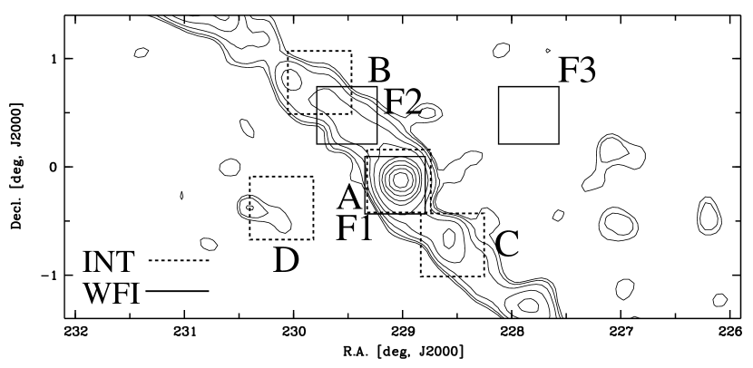
Figure 1.— Observed fields, overlaid on a contour map of the stellar surface density of Pal 5 from SDSS data (Odenkirchen et al. 2003).

Table 2Summary of the observations.

Field	$\alpha$	$\delta$	Instrument	Exp. time	Date
	(J2000)	(J2000)	& Filter	[s]
Pal 5 center (F1)	15 16 21	$-$00 10 48	WFI R	5$\times$600	2001 May 18
			WFI V	5$\times$900	2001 May 18
Northern tail (F2)	15 18 10	$+$00 31 48	WFI R	5$\times$600	2001 May 17
			WFI V	5$\times$900	2001 May 17
Control field 1 (F3)	15 11 12	$+$00 31 48	WFI R	5$\times$600	2001 May 18
			WFI V	5$\times$900	2001 May 17
Pal 5 center (A)	15 16 05	$-$00 06 36	INT B	2$\times$1000	2001 Jun 23
			INT r	3$\times$900	2001 Jun 23
Northern Tail (B)	15 19 00	$+$00 48 00	INT B	2$\times$1000	2001 Jun 24
			INT r	3$\times$900	2001 Jun 24
Southern Tail (C)	15 14 07	$-$00 42 00	INT B	2$\times$1000	2001 Jun 25
			INT r	3$\times$900	2001 Jun 25
Control field 2 (D)	15 20 24	$-$00 22 12	INT B	2$\times$1000	2001 Jun 26
			INT r	3$\times$900	2001 Jun 26

2.3. Photometric reduction

2.3.1 Basic reduction

The raw data files were split into four (INT WFC) or eight (WFI) single images, respectively, each corresponding to one individual CCD chip. Thus, during all of the subsequent reduction steps, each of the chips was treated separately. The standard reduction steps were carried out using the IRAF package. Readout bias was removed to first order by subtracting a fit of the overscan region from the frames. Any residual bias was subtracted using a mean over approximately 30 bias frames. Flatfield calibration was carried out using the qualitatively best of the observed twilight flats. Finally, bad pixels and columns were masked out. Neither dark current nor fringing causes any considerable effect in either our WFI and INT observations.

2.3.2 WFI Photometry

Details of the photometric processing and calibration of the WFI frames are described in a separate paper (Koch et al. 2004). Basically, the reduced frames were processed using the DoPHOT package (Schechter, Mateo & Saha 1993). The actual photometry was calculated by fitting an analytic point spread function to all detected objects. As we are only interested in stars for our following work, we rejected all non-pointlike objects from our photometry list. Afterwards V and R output data were matched against each other regarding position on the images, retaining only objects detected in both filters. Since the WFI does not produce entirely spatially homogeneous photometry due to central light concentration (e.g., Manfroid, Selman & Jones 2001; Koch et al. 2004), we applied photometric correction terms to remove large-scale spatial gradients. These correction terms were derived by comparing our instrumental magnitudes to the well-calibrated sample of stars from the SDSS Early Data Release (EDR, Stoughton et al. 2002), which coincide with our fields. For this purpose we defined equations of the kind

$$R^{\ast} \,=\, r+\alpha_{R}\,(g-r)\,+\,\beta\,(r-i)\,+\,c_{R},$$ (1)

$$V^{\ast} \,=\, g+\alpha_{V}\,(g-r)\,+\,c_{V},$$ (2)

with g, r, and i being SDSS magnitudes. WFI instrumental magnitudes are denoted by an asterisk. The remaining residuals after applying the transformation equations (1, 2), $\varepsilon$, showed strong spatial dependence and were fitted by a second order model ($\varepsilon=\varepsilon(x,y)$), which then was subtracted from the instrumental magnitudes. Finally, the transformation to standard Johnson magnitudes was obtained from Table 7 of Smith et al. (2002), where sets of transformation equations between the SDSS and Johnson standard systems are provided. Accounting for zero-point offsets between our data and the tabulated values of Smith et al. (2002), we get

$$R \,=\, R^{\ast}\,-\,c_{R}\,-\,\varepsilon_{R}(x,y)$$ (3)

$$V \,=\, V^{\ast}\,-\,c_{V}\,-\,\varepsilon_{V}(x,y).$$ (4)

The actual values of the coefficients ($\alpha,\,\beta$) and zeropoints ($c$) are tabulated for each of the eight WFI CCDs in Koch et al. (2004), together with the spatial model for the variations in $\varepsilon(x,y)$.

2.3.3 INT Photometry

DAOPHOT and ALLSTAR (Stetson 1987, 1994) were used to obtain the stellar photometry. To avoid contamination with background galaxies, we imposed the following constraints on crucial ALLSTAR parameters: CHI$\,<\,$2 and $-1<\,$SHARP$\,<1$. This basically rejects extended objects and merely leaves point sources with stellar point spread functions. To transform these data to a standard photometric system we proceeded analoguously to Sect. 2.3.2, i.e., by comparing our set of instrumental magnitudes to the SDSS EDR photometry, which may be regarded as a set of local tertiary standards and which overlap fully with our observed fields. INT’s r-filter is identical to the SDSS r-definition, hence a linear fit yielded the transformation to the standard SDSS sytem for each chip.

The B-magnitudes were converted into Johnson magnitudes similar to eqs. (1,3), where B is written as a linear combination of u, g and r, again with final account for offsets when compared to Smith et al. (2002).

The formal transformation errors from the fit dispersion are smaller than 0.01 mag for each chip and likewise for the zero-point error from the comparison with Smith et al. (2002) thus placing an estimate of approximately 0.02 mag on this error source. Additionally, DAOPHOT provides a dispersion of the PSF fitting for each star. These uncertainties $\sigma$ are (0.005, 0.008, 0.015, 0.035, 0.1) on average at B = (20, 21, 22, 23, 24) mag. Putting all these errors together, the total photometric error of our data can be estimated to be no larger than 0.15 mag at the very faintest magnitude bin that is going to be used in the subsequent analyses. Due to, e.g., the stronger spatial variations in the WFI photometry the respective uncertainties are larger, reaching approximately 0.2 mag at the faint end.

3. Color-magnitude diagrams and number counts

3.1. Color-magnitude diagrams

The diagrams presented in Figures 2 (WFI data) and 3 (INT data) contain data of all stellar objects found in the observed fields. The INT data reach magnitudes fainter by approximately 1 mag than the WFI data. The main sequence seen in the INT data is significantly narrower than that derived from the WFI observations, which we ascribe to the better seeing, larger color baseline, fainter magnitude limits, and hence better signal to noise of the INT data. Despite the limitations of the WFI data quality we chose to keep them for further analysis. These data do not only provide a second control field for estimating field star contamination, but also cover a different part of the tidal tails than the INT data.

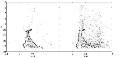
Figure 2.— Color-magnitude diagrams (CMDs) of different regions observed with the WFI. The left panel shows stars within one core radius (3$\farcm$6, field F1), whereas the CMD of field F2 in the northern tail is shown in the right panel. Additionally shown is the 2$\sigma$-envelope around the observed, averaged main sequence from the central part of the cluster that will be used for an assessment of the field contamination in Section 3.3.

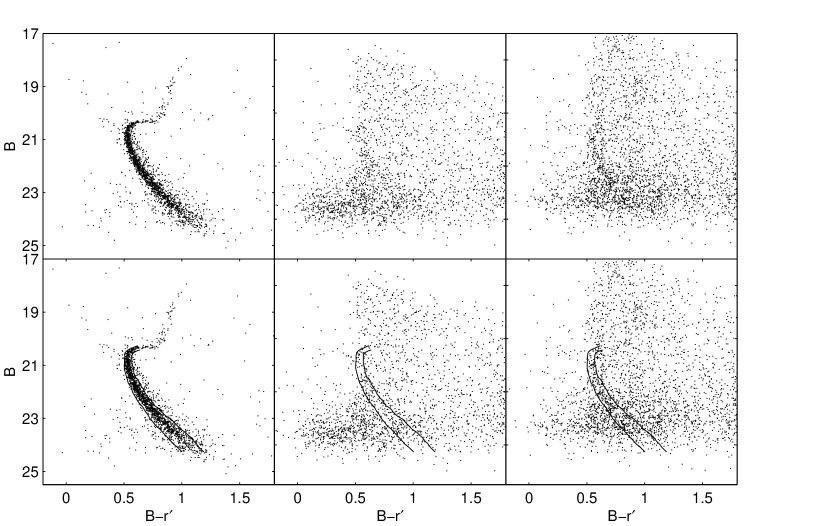
Figure 3.— Same as Figure 2, but for data taken with the INT: Left panels show the central region, middle panels display stars from field B in the northern tail, whereas the CMD for the southern tail is depicted on the right hand side. The lower panel additionally shows the 2$\sigma$-envelope of the main sequence.

The basic features of the color-magnitude diagrams (CMDs) are as follows.

1. Cluster population (left panels): Within the core radius of Pal 5 of 3$\farcm$6, the contamination with field stars is rather small ($\sim 4$%). Thus the CMD contains mainly stars belonging to the cluster population. Characteristic features are the main sequence of unevolved stars below V$\approx$20 mag, the turnoff-point at V$\approx$20.8 (Smith et al. 1986) and the narrow subgiant branch. The red giant branch is visible, although sparsely populated (see also Odenkirchen et al. 2001). Obvious horizontal branch stars are not present in our CMDs. Redward of the main sequence, there is a binary sequence visible in the INT data, which will be investigated in more detail in Sect. 6.

2. Tail population (middle/right panels): As the sparsely populated regions in the tails contain a large fraction of field stars, the signature of the evaporated cluster stars does not stand out clearly. However, the main sequence within the southern tail is more distinct than that of the northern tail, which may be due to the closer distance of field C to the cluster (at 3.3 tidal radii compared to 4.3 radii for field B). As was shown by Odenkirchen et al. (2002), the density declines with increasing distance from the cluster’s main body.

3.2. Incompleteness

In order to account for incompleteness effects in our data we performed artificial star experiments. The magnitudes of the stars added to the WFI frames were chosen to cover a range of 20.25 to 23.25 mag in steps of 0.5 mag, which we defined as central value for each magnitude interval [V$-0.25$,V$+0.25$]. One star-added image was produced for each magnitude bin for each initial image and again for each of the eight WFI chips. The artificial stars were spatially distributed on a predefined grid such that their total number amounts approximately 10% of the stellar objects found by DoPHOT on the initial frames. This procedure was chosen to avoid introducing artificial crowding (Andreuzzi et al. 2001).

Colors and magnitudes chosen for 9000 artificial stars on the INT images were obtained from an isochrone resembling the observed main sequence (11.2 Gyr, [Fe/H]=$-$1.30, see Section 5) and distributed on a grid across the entire images. Afterwards all star-added frames were processed through the DoPHOT and DAOPHOT routines using exactly the same parameter set as in the original reductions. An artificial star was defined as recovered if it met two conditions: Firstly, its position had to be identical (to within the fitting uncertainties) to the input grid position. And secondly the output magnitude was required to still lie within the input magnitude bin.

We define the limiting magnitude as the magnitude where the incompleteness fraction $\chi$, defined as the number ratio of stars recovered to those injected, drops below 50% and find V_lim = 23 mag for our WFI data and a limiting B-band magnitude of B${}_{lim}\approx 24$ mag for the INT frames. The incompleteness fraction versus B- and V-magnitude (INT and WFI, respectively) is presented in Fig. 4.

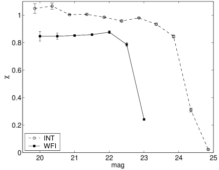
Figure 4.— Photometric completeness fraction $\chi$ for the WFI frames versus V-magnitude for one sample frame (solid line). The dashed line represents values for $\chi$ from our artificial star experiments on the INT data.

3.3. Field contamination

In order to count cluster main-sequence star candidates, it is necessary to statistically remove field star contamination. This was done in two steps. First, the mean locus of the main sequence was calculated by averaging the photometric data of stars within the cluster’s core radius (left panels of Figs. 2,3). Stars obviously not belonging to the cluster (e.g., thick disk stars at B$-$r$\,\gtrsim$ 1.3) were excluded from the averaging process. Afterwards an envelope comprising two standard deviations (2$\sigma$) of this averaged main sequence fiducial was calculated for each magnitude bin. The bin size for this process was chosen to be 0.1 mag. Finally, this 2$\sigma$-envelope was smoothed in order to encompass a maximum number of obvious cluster members. This 2$\sigma$-method for defining the cluster in color-magnitude space and transferring it to other fields provides a compromise between a complete estimate of the cluster population and minimizing the field contamination.

Table 3Field star contribution

	Central 3$\farcm$6		Northern Tail		Southern Tail	Comparison field
Field $i$	INT (A)	WFI (F1)	INT (B)	WFI (F2)	INT(C)	INT (D)	WFI (F3)
N($i$)	1701	669	525	615	451	170	869
$\frac{A_{i}}{A_{Field}}$	0.040	0.036	1.013	0.47	1.013	1	1
N($Field$)$\cdot\frac{A_{i}}{A_{Field}}$	7	31	172	408	172	170	869

However, we will inevitably enclose field stars located within 2$\sigma$-limits of the main sequence. To correct for this residual contamination, observations of two comparison fields (F3 and D) were taken. The number of stars in the respective magnitude bin in the comparison fields was subtracted from the number of stars in the science fields, weighted by the ratio of areas covered. The fractional importance of contaminants is almost negligible if one restricts the data to the region enclosed within the core radius (4%), but it accounts for a considerable fraction of stars the farther one proceeds outward from the cluster center (where the area weights are $\sim$50%, 100% respectively – see Table 3).

To get an estimate for the magnitude of field contamination in each of the observed regions (labelled $i$), Table 3 gives an overview over the total number of stars N($i$) enclosed within the 2$\sigma$-envelope down to the completeness limit and the ratio of the covered areas ($A$), which – combined with the density of cluster stars – is a measure of the fractional contribution of field stars. Also listed is the number of field stars that is statistically expected in each region, which is given by the number N($Field$)$\cdot\frac{A_{i}}{A_{Field}}$.

4. The luminosity functions

We derive the LF from number counts in field $i$ in bins with a size of 0.5 mag. Regarding this bin size, the small photometric uncertainties (see Sect. 2.3.3) do not introduce larger errors in the final LFs due to bin migration. Such an effect would only affect the data at fainter magnitudes, where the incompleteness already becomes severe. Accounting for incompleteness and field contamination, we define the LF in the B band as

$$LF_{i}(B)\,=\,\frac{N_{i}(B)}{\chi_{i}(B)}\,-\,\frac{A_{i}}{A_{Field}}\,\frac{N_{Field}(B)}{\chi_{Field}(B)}$$ (5)

and likewise for the V band. Here $N$ is the number of stars recovered per bin and $A$ is the corresponding area of the field. As the only uncertainties we assume purely statistical errors in the number counts and the incompleteness estimates. The errors in the counts are assumed to follow a Poisson distribution, whereas uncertainties in the determination of $\chi$ are derived from a binomial distribution (see Bolte 1989; Andreuzzi et al. 2004). Conversion from apparent to absolute magnitudes was obtained using a distance modulus of (m$-$M)${}_{V}=\,$16.9 and a reddening of E(B$-$V) = 0.03 (Harris 2003).

Our completeness-corrected, field-subtracted stellar main sequence LFs both for stars within Pal 5’s core radius and in the tidal tails are listed in Tables 4 (WFI) and 5 (INT). These LFs are illustrated in Figs. 5 and 6.

Table 4WFI Luminosity Functions

	Cluster Center		Tidal Tail
V	N	LF	N	LF
20.0	19	21.6	14	6.4
20.5	65	76.1	21	13.2
21.0	103	121.2	31	22.6
21.5	114	132.8	53	30.8
22.0	120	128.0	119	62.7
22.5	165	153.8	238	72.8
23.0	246	153.9

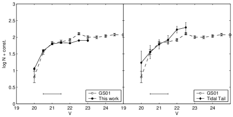
Figure 5.— Left panel: Completeness and field star corrected WFI luminosity function (LF) in [V,V+0.5] for radii $r<r_{c}$. Data from GS01 are shown as a dashed curve. These comprise both their core and off-center field. The solid line at the bottom indicates the magnitude interval used for normalization of the LFs. The right panel displays our results for the northern tidal tail, also compared to the central LF from GS01. Errorbars derive from Poisson errors in the number counts.

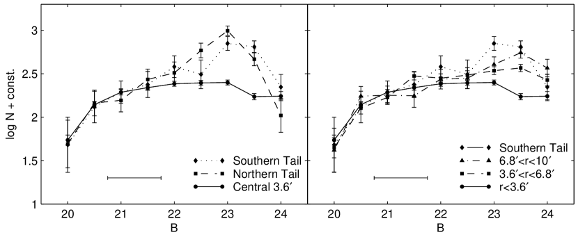
Figure 6.— Same as Fig. 5, but based on INT data. Left panel: Comparison of the cluster center and both tidal tails. Right panel: LFs in different annuli around Pal 5’s center. For the ease of comparison, the curves were normalized to fit the LF of the central region at the bright end.

Table 5INT Luminosity Functions

	Cluster Center		Northern Tail		Southern Tail		$3\farcm 6\leq r\leq 6\farcm 8$		$6\farcm 8\leq r\leq 10\arcmin$
B	N	LF	N	LF	N	LF	N	LF	N	LF
20.0	58	54.4	10	5.6	9	4.7	18	16.7	6	5.2
20.5	142	139.4	25	16.6	21	12.7	49	47.7	23	21.6
21.0	195	193.7	24	17.8	25	18.8	64	63.2	23	22.1
21.5	217	218.6	50	31.1	42	23.0	112	111.9	24	21.8
22.0	235	242.6	70	36.9	70	36.9	104	105.5	37	33.9
22.5	244	248.2	113	67.0	77	30.1	115	114.5	40	34.8
23.0	238	250.7	144	112.9	102	68.4	124	128.7	52	50.1
23.5	149	172.2	55	53.1	63	62.4	120	138.3	60	68.2
24.0	73	174.6	5	12.0	9	21.5	42	100.4	19	45.4

For comparison the combined results from both the central fields in GS01 are also shown in the WFI plot. We chose to normalize each LF to the curves from the central parts at the bright end using a simple least-squares algorithm (Piotto, Cool & King 1997) in the magnitude range from V=20.5 mag to V=21.5 mag (likewise for B), as indicated by a solid bar at the bottom of the diagrams.

4.1. Central region

Generally, our WFI observations are in good agreement with the V-band LF from GS01, thus confirming the flattening of the LF towards the faint end (M${}_{V}\gtrsim 4$) in a region located within the core radius. This trend is also visible in the INT data (Fig. 6). If we confined our data to the same region as covered by the HST in GS01, we find that our LFs coincide with those from GS01 to within the uncertainties. One should note that the “faint end” in our work is far brighter than the limiting luminosity reached by GS01, as their LF extends out to M${}_{V}=10.1$. Yet our curves drop below the HST-based reference LF in the faintest magnitude bins of our ground-based observations, leading to an even more pronounced flattening. However, it cannot be ruled out that this is caused by increasing incompleteness or difficulties in accounting for field contamination in these faint-magnitude bins. GS01 did not apply any correction for field star contamination. Field stars were only excluded by a hand-drawn main-sequence envelope, similar to our 2$\sigma$ envelope. Thus there may be remaining contamination of the main sequence with non-cluster members in the stellar sample of GS01. Another difference is that of the area sampled. The HST field of view covered by the GS01 data is $3\farcm 4$ squared whereas our LF of the central region covers $6\farcm 4$ squared, leading to an improved statistics of our larger sample.

In the brightest bin (V=20 mag) our scaled number exceeds the reference curve, a fact that can possibly be attributed to a preferential saturation of the HST data for brighter stars as well as to statistical fluctuations because of the small number of stars at brighter magnitudes. One distinctive feature of GS01’s LF is a dip at M_V=5.6 mag, which does not coincide with our WFI data within GS01’s statistical (Poisson) uncertainties. Considering the larger area covered of our analysis it appears more likely that the LF flattens constantly towards the faint end, which is strengthened by the fact that this trend is present in data taken with two different instruments. This flattening points to a strong deficiency of Pal 5’s core in low-mass stars.

4.2. Tidal tails

After statistical removal of field contamination in the entire fields B and C, and also in the WFI field F2, there still was a non-zero number of stars present. Complementary to the previous selection in color-magnitude space, these can be statistically ascribed to the cluster population.

In contrast to the LF of Pal 5 itself, the LFs of the tidal tails are rather steep compared to the LF of the cluster center at the faint end, i.e., the tails contain a higher fraction of low-mass stars than the central region of the cluster. The LFs of the tails agree within the uncertainties indicated by the error bars (left panel of Fig. 6).

The strong decline in the LFs of both streams at B$\gtrsim$23.5 is due to systematic effects because of incompleteness effects and field contamination and is not believed to be a real levelling off at that point. To test the relevance of outliers and to explore whether the differences between the northern and southern tail are significant, we applied a Kolmogorov-Smirnov (KS) test the three samples presented in Fig. 2. The test was truncated at B=23.5 mag, where incompleteness effects become severe. We find a probability of 57% that northern and southern tail are drawn from the same population. Thus the results from both northern and southern stream show consistently a similar, high degree of enhancement in low-mass stars within the uncertainties. On the other hand, the KS probability is practically zero for the hypothesis that the tails and the cluster center have the same luminosity distribution.

In order to estimate the degree of depletion or enhancement of faint stars in terms of LF flattening, we performed an error-weighted least squares fit of a power-law function to our observed LFs. The LF of the cluster center is the flattest ($x=-0.65\pm 0.22$) compared to those of the northern and southern tail ($x=4.7\pm 0.7$ and $x=3.3\pm 0.8$) at the faint end, i.e., for $21\leq$B$\leq 23.5$. These numbers suggest a distinct steepening of the tails’ LF compared to that of the core.

This is the first evidence of mass segregation effects in this cluster: The tails, composed of stars evaporated from outer regions of the cluster, contain a higher fraction of faint stars. Since the tidal shocks removed at first stars from these outer regions, there must have been a pre-existing differentiation in the stellar mass distribution between the central part and the outskirts of the cluster. This conjecture is consistent with the observed depletion of faint stars in the core of Pal 5.

4.3. Mass segregation within Palomar 5

In order to look for further evidence of mass segregation in terms of a radial variation of the LF, number counts were performed in two additional regions around the cluster center on our INT data. These consist of two annuli each of which has a width of 3$\farcm$2. This width was chosen in order to ensure that the annuli cover roughly the same area. The LFs derived for these regions are given in Table 5 and shown in the right panel of Fig. 6. There is a gradual rise in slope with increasing distance from the cluster center, starting with the strongly flattened LF of the central cluster population via the annuli’s LFs toward the low-mass-enhanced function of the tail. Power-law fits in the same magnitude range as used above yield indices of $x=1.3\pm 0.4$ and $x=2.1\pm 0.7$ for $3\farcm 6<r\leq 6\farcm 8$, $6\farcm 8<r\leq 10\arcmin$, respectively.

A KS-test revealed a probability of $<3\%$ that stars in the annuli and in the center are drawn from the same population. Hence we find our conjecture of mass segregation within Pal 5 confirmed (which then also permeates to the tails). GS01 did not find any evidence of spatially varying segregation, but they concentrated on a small region (within our central field) in the cluster center itself and did not have coverage that would have permitted them to analyze the outer cluster regions.

5. Mass functions

In order to be able to unambiguously compare our results, which were obtained in different photometric bands, we convert luminosities into masses using the M/L relations of Girardi et al. (2002, 2004). These relations offer the advantage of being available in several photometric systems and thus to be well suited for our purposes, and reproduce well the observed main sequences in the WFI and INT data. Isochrones with an age of 11.2 Gyr and a metallicity of [Fe/H]=$-$1.30 were chosen, since these values represent Pal 5’s actual characteristics (see Table 1) and yielded satisfactory results.

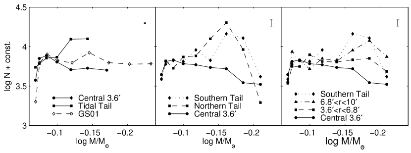
Figure 7.— Mass Functions for all observed regions in Pal 5, translated from the LFs in Figs. 5, 6 using M/L relations from Girardi et al. (2002, 2004) for 11.2 Gyr and [Fe/H]=$-1.30$. The left panel shows the WFI based data, whereas the middle and right panels display MFs derived from the INT LFs, each scaled to fit the low-mass end of the cluster center. Typical error bars derived from the number counts are indicated.

In Fig. 7 we compare the mass functions (MFs) derived from the V- and B-band LFs of all regions as presented in Section 4. As before, the curves were normalized to the curve of the cluster center at the high-mass end. The magnitude range covered by our observations corresponds to a mass range of $M=0.58-0.86\,M_{\sun}$. Errors in the mass functions were adopted from the LFs and propagated through the M/L relations.

Neither one of the curves is particularly well described by a power law over the mass range in question. Still, to assess the significance of the low-mass-star depletion of the cluster core in comparison with the tails, we determined best-fit power law indices for masses below 0.82$\,M_{\sun}$. These values are:

$$x\, = \,-0.48\pm 0.04\mathrm{,\quad GS01}$$

$$x\, = \,-0.63\pm 0.20\mathrm{,\quad WFI,\,\,r<3\farcm 6}$$

$$x\, = \,-0.63\pm 0.11\mathrm{,\quad INT,\,\,r<3\farcm 6}$$

$$x\, = \,\,\,\,\,\,0.77\pm 0.17\mathrm{,\quad INT,\,\,3\farcm 6<r\leq 6\farcm 8}$$

$$x\, = \,\,\,\,\,\,0.90\pm 0.31\mathrm{,\quad INT,\,\,6\farcm 8<r\leq 10\arcmin}$$

$$x\, = \,\,\,\,\,\,0.97\pm 0.36\mathrm{,\quad INT,\,\,Southern\,\,Tail}$$

$$x\, = \,\,\,\,\,\,1.31\pm 0.35\mathrm{,\quad INT,\,\,Northern\,\,Tail}$$

$$x\, = \,\,\,\,\,\,1.35\pm 0.82\mathrm{,\quad WFI,\,\,Tail\,\,(Field\,\,F2)}$$

In this notation, $x=1.35$ is the power-law slope of a Salpeter MF. The MFs from all observations of the central parts of Pal 5 show a high degree of flattening and good agreement within their uncertainties. Although our data cover only the higher-mass range of the main sequence, the resulting slopes are consistent with the estimate of Pal 5 having a MF index no larger than $-0.5$ (GS01). The slopes of the tidal tails, on the other hand, differ considerably from the cluster center, and their formal errors indicate a high degree of significance. It is worth noticing that the MFs of the outermost regions in the tidal tails approach the classical Salpeter MF with slopes around 1.35. Similarly, here the values are consistent with Kroupa’s (2001) multiple-part power-law MF of $x=1.3\pm 0.3$ in the mass range of $0.5$ M${}_{\odot}<M<1.0$ M_⊙. The mass segregation between cluster and tails is well confirmed by the MFs.

6. Photometric Binaries

Figure 2 (left panels) and Figure 8 show a fairly well-defined sequence of stars redward of the main sequence of Pal 5, which we ascribe to binary stars.

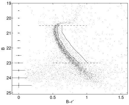
Figure 8.— CMD of stars within $3\,r_{c}$. The solid line is the same 2$\sigma$ envelope as in Fig. 2, shifted by 0.75 mag to encompass the binary main sequence. Dashed lines mark the magnitude limits within which we carried out the analysis of the secondary sequence. At the left edge of the diagram typical photometric errors are displayed.

In principle, other effects such as rotation (e.g., Collins & Sonneborn 1977; Grebel, Roberts, & Brandner 1996) can also account for a color and magnitude shift in the locus of main-sequence stars, but these affect primarily high-mass stars. Rotational velocities of unevolved stars in globular clusters have been found to be low (Lucatello & Gratton 2003).

Only certain types of binaries can be distinguished as “photometric binaries” because of their location in a CMD. Binaries with large mass ratios will be embedded within the primary main sequence (Hurley & Tout 1998; Elson et al. 1998). A visible binary sequence will be composed primarily of stars with a mass ratio of $q>0.6$ (Pols & Marinus 1994). We will miss wide-separation binaries whose components are resolved in our photometry, although these should only contribute sparsely. In the following, we will call only those stars “binaries” whose photometric properties place them at a location outside of the chosen $2\sigma$-envelope around the main sequence. Hence our binaries are at best a subset of the true number of binaries.

In order to estimate the stellar content of the binary sequence, we performed number counts similar to those described in Sect. 4. Since the mean locus of the secondary main sequence should be shifted by no more than 0.75 mag (unevolved equal-mass binaries) toward brighter magnitudes, we chose to shift the 2$\sigma$-envelope by this maximum amount and counts of binary candidates were obtained within this shifted envelope. As the CMD in Fig. 8 implies, the observed binary sequence can be excellently accounted for by this shift, and there is no apparent overdensity near the main sequence that would correspond to a magnitude shift of more that 0.75 mag. We confined our analysis to the magnitude range $20.5<B<23$, where the secondary main sequence is defined most clearly. Field star contamination was accounted for in the usual way via counts in the identical region of the CMD of the comparison field D.

Another source of data points that appear to be photometric binaries is crowding. Regular main-sequence stars may be scattered away from the primary sequence due to their photometric errors (see Fig. 8) and pollute the second sequence, hampering the determination of the cluster’s true binary content.

Crowding and blends will particularly contribute to these spurious binaries (Walker 1999). On the other hand, Pal 5 is a very loose, sparse cluster with little crowding, so one would expect less of an effect than in more typical, rich, dense globular clusters.

In order to test the possibility of photometric scatter as the major source of the redward spread in the CMD, we divided our data into two samples following the procedure employed by Walker (1999): “Sample 1” was purged of stars with standard errors (as determined by DAOPHOT) larger than two median standard errors of all stars within a given magnitude bin of 1 mag width. Yet this procedure only removed a few outliers and is thus basically identical to the inclusion of all stars. Our “sample 2” contains only those stars within two standard deviations of the mean of the photometric errors. Additionally, the data were cut off at standard errors greater than 0.02 mag, thus forming a low-error “sample 3”. This cut basically removes stars with B $\gtrsim 22.5$ mag. For all samples, we determined the distribution of colors around the main sequence fiducial. As the left panel of Fig. 9 shows, neither of the distributions is symmetric across the peak. Each distribution shows a clear excess of stars with redder colors. The difference between the three samples is small, and the samples 1 and 2 are almost identical. Sample 3 exhibits a narrower color distribution both blueward and redward of the fiducial. This behavior is different from what was found by Walker (1999) for the rich globular cluster NGC 2808.

The same procedure was carried out on our artificial star sample, which is shown in the right panel of Fig. 9. Also these distributions are asymmetric and all show an excess in numbers toward redder colors. Again, the samples 1 and 2 are essentially indistinguishable. Only sample 3 shows a slightly reduced red excess.

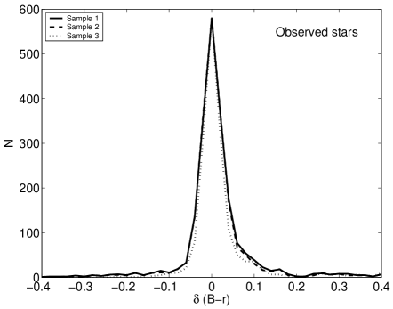
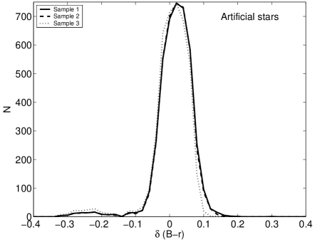
Figure 9.— Histograms of the colour distribution of stars around the MS fiducial (normalized to the peak values). On the left side, observed stars from our INT data are shown. The three samples were drawn from stars within 3 core radii according to cut offs in their photometric errors. The right panel displays the respective results from our artificial star experiments.

We conclude that photometric scatter alone cannot explain the secondary sequence seen in the CMD, since also the observed low-error samples unequivocally exhibit such a feature. Furthermore, the differences between sample 2 and 3 indicate that photometric scatter becomes mainly significant at B $\gtrsim 22.5$ mag.

It is worth noticing, however, that the color distribution of the artificial stars is generally more dispersed towards the red: Its average of 0.015 mag (with a 1 $\sigma$-width of 0.04 mag) compares to an average of practically zero (and a width of 0.02 mag) of the distribution of INT-observed stars. One reason for this shift is the high occurrence of red field stars (see our CMDs, Fig. 3), resulting in a larger probability that an artificial star will blend with such a red star (Aparicio & Gallart 1995). This will yield a redder color of the recovered star.

6.1. Radial variations in binary fractions versus single stars?

We define the binary fraction $f_{b}$ as the field- and completeness-corrected number ratio of binary candidates within the shifted $2\sigma-$envelope to the combined number of binaries and prima facie single stars (primary sequence within the original 2$\sigma$-region). In the cluster center, i.e., for $r<r_{c},\,f_{b}$ is found to be (9 $\pm$ 1)%, with the uncertainty being purely based on (Poisson-) uncertainties in number counts. This is a value in good agreement with typical globular cluster binary frequencies of 3–30% (see reviews of Hut et al. 1992; Meylan & Heggie 1997, and references therein). There is now strong evidence that most globular clusters began their lives with a significant primordial binary content of at least 10% (McMillan, Pryor & Phinney 1998). Moreover, low density globular clusters suffering from extensive tidal mass loss have been shown to maintain a fraction of soft binaries at the high end of this observed range (Yan & Cohen 1996; McMillan et al. 1998). Under elaborate assumptions about the binary mass spectrum and orbits, Odenkirchen et al. (2002) simulated the behavior of binaries in Pal 5 and estimated $f_{b}$ to be roughly (40 $\pm$ 20)%, which is significantly higher than our observations imply. This may be due to our insensitivity to binaries that are not near-equal-mass pairs. Hence, a concise determination of binary fractions necessitates allowance for their mass ratios or the use of statistical methods (Bellazzini et al. 2002a), but this is beyond the scope of our rough photometric estimate.

To determine radial variations in the occurrence of binaries, the secondary sequence was analyzed out to 3 core radii. The resulting values for $f_{b}$ are illustrated in Fig. 10.

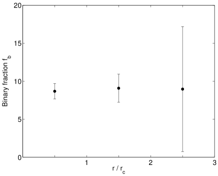
Figure 10.— Estimated binary fraction as measured in concentric annuli around the center of Pal 5: $r\leq r_{c}$, $r_{c}<r\leq 2\,r_{c}$ and $2\,r_{c}<r\leq 3\,r_{c}$. Also indicated are Poisson error bars.

In the outer parts of the cluster, $f_{b}$ is (9 $\pm$ 8)% for $2r_{c}<r<3r_{c}$, hence the uncertainties here are too large to permit a meaningful measurement. Within two core radii, the binary fraction remains roughly constant as a function of radius within the uncertainties. Based on these data we do not find evidence of mass segregation in the binary component as a function of radius in the sense that more binaries are residing in the central region.

6.2. Radial variations in binary masses?

Finally, we consider the question whether more massive binary systems differ in their radial distribution from that of less massive ones. To distinguish between the two, we adopt a simple luminosity cut and then measure the ratio N${}_{b}(20.5<B<22)$/N${}_{b}(22<B<23)$ within different radial bins. These cuts correspond to approximate mass ranges of $0.76-0.84\,M_{\odot}$, $0.69-0.76\,M_{\odot}$, respectively. Between two and three core radii, number statistics are too poor. In the annulus within one core radius, we find a ratio of $1.00\pm 0.25$ and in the annulus ranging from two to three core radii, this ratio is $0.55\pm 0.25$. This compares to 1.12$\pm$ 0.07 and 1.01$\pm$ 0.11 in the same two annuli for stars on the primary main sequence. While the ratios do not vary much along the “single”-star main sequence, the binary ratios may indicate a tendency for more massive binaries to be more centrally concentrated (although the uncertainties are large).

6.3. Binaries: primordiality versus dynamical evolution

The origin of the binaries can be explored by comparing rates of the processes that produce binaries (Bellazzini et al. 2002a). Tidal captures should only have contributed marginally during Pal 5’s evolution, regardless of the environment in which the cluster resided (i.e., at apocenter in the halo or during disk shocks). The latter becomes obvious when inserting Pal 5’s low velocity dispersion $\sigma$ and respective estimates for the stellar density $\nu$ into the formula by Lee & Ostriker (1986)

$$t_{tid.capt.}\,\approx 10^{12}\,yr\,\times\,\left(10^{5}\,pc^{-3}/\nu\right)\,\left(\sigma/100\,km\,s^{-1}\right)^{1.2}$$

(after Binney & Tremaine 1994) – both assuming the current value (Odenkirchen et al. 2002, 2003) and allowing for a variation of an order of magnitude. The resulting capture rates are less than 1 over Pal 5’s present age. The rate of binary systems forming by three-body interactions is estimated to be $\sim 0.1/(N\ln N)$ per relaxation time (Binney & Tremaine 1994). Using Pal 5’s total present-day mass of $\sim 5000$ $M_{\sun}$ (Odenkirchen et al. 2002) and an average stellar mass of 1 $M_{\sun}$, this corresponds to $\sim 10^{-7}$ during the cluster’s lifetime. Hence, the most likely origin of Palomar 5’s binary population is primordiality if the present properties of Pal 5 are representative of its past mass and density, and if the cluster is in dynamical equilibrium.

Dehnen et al. (2004) argue that the large size and low concentration of Pal 5’s main body are due to expansion after the last disk shock. They note that Pal 5 is at least two times larger than its theoretical tidal radius. The internal dynamical time scales of Pal 5 exceed the time between disk passages, so that the external tidal shocks dominate the dynamical evolution. Pal 5 may have been already a low-concentration, low-mass cluster to begin with, which together with its highly eccentric orbit would have facilitated its dissolution. Extrapolating back, Dehnen et al. (2004) estimate Pal 5’s original mass to have been $\leq 70,000$ M_⊙. The estimates provided by these authors again suggest long dynamical time scales with a two-body relaxation time of $\sim 20$ Gyr. This, too, then supports the assumption that the binaries in Pal 5 and its mass segregation are largely primordial. On the other hand, Dehnen et al.’s (2004) N-body simulations only cover a few Gyr, and they caution that extrapolating back further may be dangerous because of the unknown changes in the Galactic disk potential. Hence it cannot be excluded that Pal 5 was initially significantly denser and did experience dynamical mass segregation.

7. Comparison with other clusters

We have shown that Pal 5’s main sequence LF is significantly deficient in faint stars compared to the LF of its tidal tails and that its mass function thus is strongly flattened. Now the question arises how this behavior compares to other globular clusters. Or in other words: how strong is the depletion of the cluster itself compared to the LF or MF of other clusters? Table 6 lists four different clusters that will be used for an illustrative comparison.

Table 6Comparison Clusters

Object	[Fe/H]	concentration	$\log\,t_{rh}$	Reference
Pal 5	$-$1.43	0.66	9.89	cf. Table 1
M 10	$-$1.52	1.40	8.86	Piotto & Zoccali (1999)
M 22	$-$1.64	1.31	9.22	Albrow, DeMarchi & Sahu (2002)
NGC 288	$-$1.39	0.96	9.26	Bellazzini et al. (2002b)
NGC 6397	$-$1.82	2.50	8.46	Andreuzzi et al. (2004)

All of these globular clusters were found to exhibit hints of flattening at the faint end of their overall LF, which becomes manifest in the comparison to a whole sample of globular clusters (e.g., Piotto & Zoccali 1999). Likewise, power-law indices of many cluster MFs tend to be fairly shallow as the comparison of the LFs of a few GCs implies (see Fig. 11).

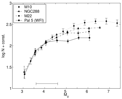
Figure 11.— Luminosity functions of Pal 5’s center (WFI data), M 10 (Piotto & Zoccali 1999), M 22 (Albrow, DeMarchi & Sahu 2002) and NGC 288 (Bellazzini et al. 2002b). M 10’s LF can be described best by a mass function with a power-law exponent $x=0.5$, whereas Pal 5’s LF is significantly flatter ($x\approx$–0.6).

Among these, M 10 is the cluster with the steepest LF (an index of $x\approx+0.5$ fits this cluster’s MF). Leon, Meylan & Combes (2000) found weak evidence for a tidal extension resulting from a recent disk crossing. They predict mass segregation, although there is no observational evidence for this effect so far (Hurley, Richer & Fahlman 1989). The differences to other clusters’ LFs are attributed to primordial differences, i.e., different IMFs, or to a moderate internal dynamical evolution, as reflected in its short relaxation time (Piotto & Zoccali 1999). The LFs of M 22 and NGC 288 are, on the other hand, distinctly flattened compared to M 10. In both these clusters, mass segregation has been established and it is known for NGC 288 that it exhibits a highly inclined and eccentric orbit making it sensitive to tidal shocks during passages close to the Galactic center (see reference in Table 6). It then appears even more remarkable that Pal 5’s LF falls below the already significantly depleted LFs of the other potentially tidally pruned clusters (although similar tidal features as around Pal 5 have yet to be detected in these clusters). This may support the suggestion by Dehnen et al. (2004) that in order to be so significantly disrupted, a cluster must have been of comparatively low mass and low concentration ab initio, whereas M22 and NGC 288 are both more compact and more massive.

The presence or absence of mass segregation is also demonstrated in Fig. 12, where we compare LFs of the globular clusters from Table 6 that were obtained at different distances from each cluster’s center.

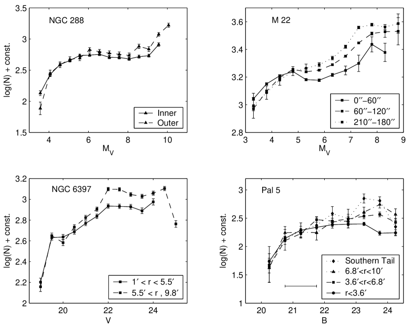
Figure 12.— Spatially resolved LFs of the clusters in Table 6, each scaled such that their number counts match one another at their bright end. The inner and outer curves of NGC 288 refer to a field near its half-mass radius (“inner”) and a region located at a larger distance from the cluster center. M 22’s LF was analyzed in annuli around the center ($r_{c}\,=\,1\farcm 4$). The data are from Bellazzini et al. (2002b) for NGC 288, Albrow, DeMarchi & Sahu (2002) for M 22 and Andreuzzi et al. (2004) for NGC 6397. Pal 5’s LF is the INT-based LF derived in the previous chapters.

A comparison of two LFs from HST observations of fields near two and three core radii in NGC 288 (top left) reveals a significant deficiency of faint stars in the inner field compared to the outer one, thus confirming the occurrence of mass segregation, which is in good agreement with the theoretical predictions (Bellazzini et al. 2002b). M 22’s LF (top right panel) has been analyzed in annuli reaching out to five core radii (Albrow, DeMarchi & Sahu 2002). There is a significant enhancement of massive stars in the core compared to the regions outside the core. As the authors show by numerical modelling, the high degree of observed mass segregation can be entirely explained by standard relaxation processes within the cluster. Various observations (Andreuzzi et al. 2004; De Marchi, Paresce & Pulone 2000; Piotto & Zoccali 1999) have shown that the core collapsed metal poor cluster NGC 6397, which is also the Galactic GC closest to us, has a remarkably flattened MF. Estimates of a power-law yielded $x=-0.5$ for the present-day MF, placing it at the lower end of the MF scale. The deficit in low-mass stars in this cluster is attributed to evaporation and tidal shocking, both effects operating simultaneously. Its vulnerability to tidal shocks is underscored by the cluster’s highly oscillating orbit (Dauphole et al. 1996), bringing it close to the dense regions of the Galacit plane near the center.

In addition to this high degree of depletion, analyses of the MFs of NGC 6397 at different radii have revealed a significant difference in the MF slope, where this mass segregation indicates that NGC 6397 is a dynamically relaxed system (see its short relaxation time, Table 6).

Hence mass segregation is a common phenomenon in globular clusters. Depending on the intrinsic cluster properties and on their orbits, it may be primordial or evolutionary; most likely a mixture of both.

8. Summary

The halo globular cluster Pal 5 is the first globular cluster around which well-defined, extended tidal tails were detected. The cluster is believed to be in the final stages of total dissolution and stands out due to its low mass, low density, and comparatively large angular extent. If Pal 5 was a low-concentration cluster to begin with, one would expect that internal dynamical effects should have had little impact on its evolution owing to the long stellar encounter time scales. Under these assumptions, one may also expect that mass segregation within the cluster would be small unless primordial mass segregation took place. External tidal effects due to disk shocks should dominate. Consequently one might expect that the mass spectrum in Pal 5’s tails would closely resemble the mass spectrum in the cluster itself.

In the present paper LFs for different regions in the globular cluster Pal 5 were measured. The LF of the cluster’s central region was found to be in good agreement with that previously published by Grillmair & Smith (2001) based on HST data. Comparison with other globular clusters shows that Pal 5’s central LF is significantly depleted in low mass stars.

We measured LFs also in various annuli around the cluster center as well as in the tidal tails of Pal 5. While the cluster center is depleted in low-mass stars, the LFs become increasingly steep with increasing distance from the cluster center, and the tidal tails are enhanced in faint, low-mass stars.

This trend is also to be seen in the mass functions that were derived from the observed LFs. With a power-law exponent of $x\approx-0.6$ Pal 5 itself is at the lower limit of globular cluster MFs. This high degree of flattening is unusual for globular clusters. Likewise, the tidal tails’ MFs differ significantly from that of the core and are similar to Salpeter’s (1955) or Kroupa’s (2001) power-law MFs.

Hence there is clear evidence of a radially varying mass spectrum and thus segregation.

Mass segregation is not obvious when investigating the distribution of photometric binary stars identified via a binary main sequence in color-magnitude space in comparison to the primary, single-star main sequence. However, more massive binary system candidates are more strongly concentrated toward the cluster center than less massive ones.

The discovery of mass segregation does not appear to be self-evident, since the time scales for dynamical mass segregation for low-concentration clusters are of the order of more than a Hubble time. On the other hand, mass segregation has been shown to occur in open clusters (e.g., Bonatto & Bica 2003 and references therein). In the case of Pal 5, it is difficult to assess how much of the observed mass segregation might be primordial and how much might be due to evolutionary effects. While we can fairly accurately determine Pal 5’s present-day mass, structural parameters, and kinematics, it remains unclear what its initial conditions were. N-body simulations by Dehnen et al. (2004) together with the mass loss rates derived by Odenkirchen et al. (2003) suggest that Pal 5 once was more than 10 times as massive than observed today (present-day mass: $\sim 5000$ M_⊙). It may have been a low-density cluster to begin with, possibly with a certain amount of primordial mass segregation. As lower mass stars would then have had a more extended spatial distribution, they would also have been more easily stripped from the cluster during disk passages. The effect of external tidal forces on cluster stars increases with their distance from the cluster center proportionally to $r^{3}$. The internal dynamics will certainly have been affected by external tides as those led to structural changes in the cluster as a whole (in particular, expansion and oscillations). Possibly external effects may even have sped up mass segregation within the cluster. Detailed N-body simulations with star particles covering a range of masses are required to explore the interplay of these effects in more detail.

References

- Aguilar, Hut, & Ostriker (1988) Aguilar, L., Hut, P., & Ostriker, J. P. 1988, ApJ, 335, 720
- (2) Albrow, M.D., DeMarchi, G., & Sahu, K.C 2002, ApJ, 579, 660
- (3) Aparicio, A., & Gallart, C. 1995, AJ, 110, 2105
- (4) Andreuzzi, G., De Marchi, G., Ferraro, F.R., Paresce, F., Pulone, L., & Buonanno,R. 2001, A&A, 372, 851
- (5) Andreuzzi, G., Testa, V., Marconi, G., Alcaino, G., Alvarado, F., & Buonanno, R. 2004, A&A subm. (astro-ph/0406309)
- (6) Bellazzini M., Fusi Pecci, F., Messineo, M., Monaco, L., & Rood, R.T. 2002a, AJ, 123, 1509
- (7) Bellazzini M., Fusi Pecci, F., Montegriffo, P., Messineo, M., Monaco, L., & Rood, R.T. 2002b, AJ, 123, 2541
- (8) Binney, J., & Tremaine, S. 1994 Galactic Dynamics, Princeton University Press
- (9) Bolte, M. 1989, ApJ, 341,168
- Bonatto & Bica (2003) Bonatto, C. & Bica, E. 2003, A&A, 405, 525
- Chabrier & Méra (1997) Chabrier, G. & Méra, D. 1997, A&A, 328, 83
- Collins & Sonneborn (1977) Collins, G. W. & Sonneborn, G. H. 1977, ApJS, 34, 41
- (13) Cousins, A.W.J. 1978, MNASSA, 37, 8
- (14) Dauphole, B., Geffert, M., Colin, J., Ducourant, C., Odenkirchen, M., & Tucholke, H.-J. 1996 A&A, 313, 119
- Dehnen et al. (2004) Dehnen, W., Odenkirchen, M., Grebel, E.K., & Rix, H.-W. 2004, AJ, 127, 2753
- (16) De Marchi, G., Paresce, F., & Pulone L. 2000, ApJ, 530, 342
- (17) Elson, R.A.W., Sigurdsson, S., Davies, M., Hurley, J., & Gilmore, G. 1998, MNRAS, 300, 857
- Girardi et al. (2002) Girardi, L., Bertelli, G., Bressan, A., Chiosi, C., Groenewegen, M. A. T., Marigo, P., Salasnich, B., & Weiss, A. 2002, A&A, 391, 195
- Girardi et al. (2004) Girardi, L., Grebel, E.K., Odenkirchen, M., & Chiosi, C. 2004, A&A, 422, 205
- Grebel (2001) Grebel, E. K. 2001, Reviews of Modern Astronomy, 14, 223
- Grebel, Roberts, & Brandner (1996) Grebel, E. K., Roberts, W. J., & Brandner, W. 1996, A&A, 311, 470
- (22) Grillmair, C.J., & Smith, G.H. 2001, AJ, 122, 3231
- Gunn et al. (1998) Gunn, J. E., et al. 1998, AJ, 116, 3040
- (24) Harris, W.E. 1996, AJ, 112, 1487
-
(25)
Harris, W.E. 2003, http://www.physics.mcmaster.ca/resources/
globular.html - (26) Hurley, J., & Tout, C.A. 1998, MNRAS, 300, 977
- Hurley, Richer, & Fahlman (1989) Hurley, D. J. C., Richer, H. B., & Fahlman, G. G. 1989, AJ, 98, 2124
- (28) Hut, P. et al. 1992, PASP, 104, 981
- (29) Johnson, H.L., & Morgan, W.W. 1953, ApJ, 117, 313
- King, Sosin, & Cool (1995) King, I. R., Sosin, C., & Cool, A. M. 1995, ApJ, 452, L33
- (31) Koch, A., Odenkirchen, M., Grebel, E.K., & Caldwell, J.A.R. 2004, AN, 325, 299
- Kroupa (2001) Kroupa, P. 2001, MNRAS, 322, 231
- (33) Lee, H.M., & Ostriker, J.P. 1986, ApJ, 310, 176
- Lee, Fahlman, & Richer (1991) Lee, H. M., Fahlman, G. G., & Richer, H. B. 1991, ApJ, 366, 455
- (35) Leon, S., Meylan, G., & Combes, F. 2000, A&A, 359, 907
- Lucatello & Gratton (2003) Lucatello, S. & Gratton, R. G. 2003, A&A, 406, 691
- (37) Manfroid, J., Selman, F., & Jones 2001, ESO Messenger 104, 16
- (38) Martell, S.L., Smith, G.H., & Grillmair, C.J. 2002, BAAS, 201, 711
- (39) McMillan, S.L.W., Pryor, C., & Phinney, E.S. 1998, Highlights in Astronomy, 11, 616
- (40) Meylan, G., & Heggie, D.C. 1997, A&ARv, 8, 1
- Murray & Lin (1996) Murray, S. D. & Lin, D. N. C. 1996, ApJ, 467, 728
- Odenkirchen et al. (2001) Odenkirchen, M. et al. 2001, ApJ, 548, L165
- Odenkirchen et al. (2002) Odenkirchen, M., Grebel, E. K., Dehnen, W., Rix, H., & Cudworth, K. M. 2002, AJ, 124, 1497
- Odenkirchen et al. (2003) Odenkirchen, M. et al. 2003, AJ, 126, 2385
- Oh & Lin (1992) Oh, K. S. & Lin, D. N. C. 1992, ApJ, 386, 519
- (46) Paresce, F., & De Marchi, G. 2000 , ApJ, 534, 870
- (47) Piotto, G., Cool, A.M., & King, I.R. 1997, AJ, 113, 1345
- Piotto & Zoccali (1999) Piotto, G. & Zoccali, M. 1999, A&A, 345, 485
- Pols & Marinus (1994) Pols, O.R., & Marinus, M. 1994, A&A, 288, 475
- Salpeter (1955) Salpeter, E. E. 1955, ApJ, 121, 161
- (51) Schechter, P.L., Mateo, M., & Saha, A. 1993, PASP, 105, 1342
- (52) Smith, G.H., McClure, R.D., Stetson, P.D., Hesser, J.E., & Bell, R.A. 1986, AJ, 91, 842
- (53) Smith, J.A. et al. 2002, AJ, 123, 2121
- Stetson (1987) Stetson, P. B. 1987, PASP, 99, 191
- (55) Stetson, P.B. 1994, PASP, 106, 250
- (56) Stoughton, C. et al. 2002, AJ, 123, 485
- (57) Walker, A. 1999, AJ, 118, 432
- (58) Yan, L., & Cohen, J.G. 1996, AJ, 112, 1489