The running-mass inflation model and WMAP

Abstract

We consider the observational constraints on the running-mass inflationary model, and in particular on the scale-dependence of the spectral index, from the new Cosmic Microwave Background (CMB) anisotropy measurements performed by WMAP and from new clustering data from the SLOAN survey. We find that the data strongly constraints a significant positive scale-dependence of $n$, and we translate the analysis into bounds on the physical parameters of the inflaton potential. Looking deeper into specific types of interaction (gauge and Yukawa) we find that the parameter space is significantly constrained by the new data, but that the running mass model remains viable.

I Introduction

The measurements of the Cosmic Microwave Background (CMB) anisotropies provided by the Wilkinson Microwave Anisotropy Probe (WMAP) mission Bennett03 have truly marked the beginning of the era of precision cosmology. In particular, the shape of the measured temperature and polarization angular power spectra are in spectacular agreement with the expectations of the standard model of structure formation, based on primordial adiabatic and nearly scale invariant perturbations. Assuming this model of structure formation, accurate albeit indirect constraints on several cosmological parameters have been reported spergel in agreement with those previously indicated (see e.g. cjo ) but with much larger error bars.

Moreover, new, complementary, results from the Sloan Digital Sky Survey (SDSS) on galaxy clustering (see e.g. Tg04 ) and, more recently, on Lyman-alpha Forest clouds (Se04 ) are now further constraining the scenario.

The question naturally arises if this new cutting-edge cosmological data can tell us something about inflation, assuming of course that the vacuum fluctuation of the inflaton generates the primordial perturbation. (If instead some ‘curvaton’ field curvaton1 ; curvaton2 does the job, the data give information mostly about the properties of the curvaton, during some post-inflationary era.) It is therefore not a surprise that several recent works have attempted to use this new cosmological data to constraint and/or falsify inflationary physics. In particular, constraints have been placed on the general form of the single field inflationary potential, for instance in WMAP-peiris , kkmr , SL03 and Se04 . A different approach is to ask about constraints on specific well-motivated models, constructed in accordance with present ideas about what lies beyond the Standard Model of the interactions. A comprehensive survey of such models has been provided treview ; book , which in general predict an almost scale-invariant spectral index $n<1$. Unfortunately, the data do not yet discriminate between these scale-invariant models Se04 .

In this paper, we study instead a specific inflationary scenario, Stewart’s running-mass model st97 ; st97bis ; clr98 ; cl98 ; c98 ; rs , a type of inflationary model which emerges naturally in the context of supersymmetric extensions of the Standard Model. The model is of the single-field type (i.e. the slowly-rolling inflaton field has only one component treview ; book ), but nevertheless it has the striking signature of a very specific and relatively strong scale dependence of the spectral index. It is therefore a natural question to ask, if such a dependence is compatible or even preferred by the present data: in fact the WMAP collaboration claimed to have a slight evidence for non-vanishing running of the spectral index in their first year data. Even if their best fit value for $n^{\prime}$ is too strong to be accommodated in the usual paradigm of slow-roll models and probably is generated mostly by the Lyman $\alpha$ Lya-run or even the low multipole data, we will attempt a conservative comparison and repeat our analysis in clm03 , on order to test the predictions of the running-mass model.

Our paper is organized as follows: In section II we discuss the running mass model. In section III we present our data analysis method and results. Finally, in section IV, we discuss our conclusions.

II The Running Mass Model

II.1 The inflationary potential

In common with all supersymmetric models, the running mass model st97 ; st97bis ; clr98 ; cl98 ; c98 ; rs chooses for the inflaton $\phi$ a flat direction, in order to suppress all the renormalizable inflaton couplings. Also, $\phi$ is many orders of magnitude less than the reduced Planck scale $M_{\rm P}=2.4\times 10^{18}\,\mbox{GeV}$ which ensures that the Planck-suppressed non-renormalizable terms are negligible. Symmetries can moreover guarantee that odd powers of $\phi$ and in particular the possible lower order linear term bcd are absent. The tree-level potential is therefore a constant $V_{0}$ plus a soft supersymmetry breaking mass term. Note then that in the running-mass model, inflation takes place in a region of field space in which one (or more) of the fields are strongly displaced from the vacuum, typically by an amount $\sim M_{\rm P}$. The model is typically a realization of Linde’s hybrid inflation linde91 , where the displaced field is a ‘waterfall field’, different from the slowly-rolling inflaton, and stabilized temporarily during inflation by an effective mass term. At tree-level, the running-mass model then reduces to the version of hybrid inflation proposed in rsg , distinguished from more general models by the fact that the waterfall field is displaced from the vacuum by an amount of order $M_{\rm P}$, and it has also a mass not far above the generic supergravity-mediated supersymmetry breaking value.

So in this setting, the inflaton potential is dominated simply by the soft supersymmetry-breaking mass term generated by $V_{0}$ and its radiative corrections. These are taken into account by using the Renormalization Group (RG) improved potential. To construct this, one just needs to substitute the tree mass with the running mass st97 ; st97bis :

$$V=V_{0}+\frac{1}{2}m^{2}(\ln\phi)\phi^{2}+\dots\,.$$ (1)

Here $m^{2}(\ln\phi)$ is obtained by integrating the RG equation of the form

$${\mbox{d}m^{2}\over\mbox{d}\ln\phi}={\mbox{d}m^{2}\over\mbox{d}\ln Q}=\beta_{m}\,,$$ (2)

with $\beta_{m}$ being the $\beta$-function of the soft inflaton mass and depending on all its couplings. A crucial assumption of the running mass model is that the radiative corrections are substantial, as they are exploited to realize slow-roll in some region of the potential. In fact at the Planck scale $\phi\sim M_{\rm P}$, the mass-squared is supposed to have the generic supergravity value $|m^{2}|\simeq H_{I}^{2}=V_{0}/(3M_{\rm P}^{2})$. The radiative corrections drive down $m^{2}$, so that, when $\phi$ is many orders of magnitude below $M_{\rm P}$, it has the much smaller value which is needed for viable inflation. There are four types of model, depending on the sign of $m^{2}$ at the Planck scale, and on whether or not that sign has changed by the time that the inflationary regime is reached.

Note that sufficiently strong running is realized for example in the case of radiative EW symmetry breaking in the Minimal Supersymmetric Standard Model, where the running turns one of the Higgs doublet’s mass from positive to negative: the main difference is that in this case it is sufficient to suppress the mass and so we do not need to rely on a very large coupling, as the top Yukawa. Unfortunately, since some of the fields take a large $M_{\rm P}$ v.e.v. after inflation, it is not viable to implement the running mass model directly within the MSSM, but possibly in some of its extensions .

In general at one loop $\beta_{m}$ is given by st97bis ; c98

$$\beta_{m}=-\frac{2C}{\pi}\alpha\widetilde{m}^{2}+{D\over 16\pi^{2}}|\lambda|^{2}m^{2}_{loop}\,,$$ (3)

where the first term arises from the gauge interaction with coupling $\alpha$ and the second from the Yukawa interaction $\lambda$. It is easy to generalize to the case of more gauge groups or Yukawas. In the expression above, $C,D$ are positive group-theoretic numbers of order one, counting the degrees of freedom present in the one-loop diagrams contributing to the running, $\widetilde{m}$ is the gaugino mass, while $m^{2}_{\rm loop}$ is the common susy breaking mass-squared of the scalar particles interacting with the inflaton via Yukawa interaction. Note that the first term in Eq. (3) is always negative, while the second has no definite sign, since $m^{2}_{\rm loop}$ is defined as the mass squared splitting between scalar and fermionic superpartners and can have either sign. Also the case of a non-interacting inflaton gives directly $\beta_{m}=0$ and it coincides with the constant mass potential. Anyway, in realistic cases the inflaton must have some interaction in order to reheat the universe or to secure a hybrid end to inflation and so in any model we expect naturally some running, even if perhaps below the level required by the running-mass model .

Over a sufficiently small range of $\phi$, or for small inflaton couplings, it is a good approximation to take a truncated Taylor expansion of the running mass $m^{2}(\ln\phi)$ around a particular scale, which we will choose as $\phi_{\rm 0}$, the inflaton value at the epoch of horizon exit for the pivot scale $k_{\rm 0}$; for comparison with the WMAP results WMAP-peiris we choose $k_{\rm 0}=0.002h\,\mbox{Mpc}^{-1}$. Then we have:

$$V=V_{0}+\frac{1}{2}m^{2}(\ln\phi_{\rm 0})\phi^{2}-\frac{3}{2}cH_{I}^{2}\phi^{2}\;\ln\left({\phi\over\phi_{\rm 0}}\right)\,,$$ (4)

where we have rescaled the last term w.r.t. $3H_{I}^{2}$ for future convenience. The dimensionless constant $c$ is proportional to the mass beta function at the particularly chosen point,

$$c=-{\beta_{m}(\ln\phi_{\rm 0})\over 3H_{I}^{2}}\,.$$ (5)

The linear expansion corresponds on the quantum field theory side to the one–loop expansion, since it practically neglects the running of $\beta_{m}$, which arises at two–loops. It has been shown cl98 that for small $c$, as is required by the slow roll conditions, this linear approximation is more than sufficient over the range of $\phi$ corresponding to horizon exit for astronomically interesting scales, i.e. between $k_{\rm 0}$ and $8h^{-1}\,\mbox{Mpc}$.

To simplify the expressions, it is very useful to introduce a new parameter $\phi_{*}$ via

$$m^{2}(\ln\phi_{\rm 0})=3H_{I}^{2}\,c\left[\ln\left({\phi_{*}\over\phi_{\rm 0}}\right)+\frac{1}{2}\right]\,.$$ (6)

Then Eq. (7) takes the simple form cl98

$$V=V_{0}-\frac{3}{2}cH_{I}^{2}\phi^{2}\left(\ln\left(\frac{\phi}{\phi_{*}}\right)-\frac{1}{2}\right)\,,$$ (7)

leading to

$$\frac{V^{\prime}}{V_{0}}=-c\frac{\phi}{M_{\rm P}^{2}}\ln\left(\frac{\phi}{\phi_{*}}\right)\,,$$ (8)

In typical cases the linear approximation is valid at $\phi=\phi_{*}$, and that point is then a maximum or a minimum of the potential.

The running-mass model supposes that all soft masses at the Planck scale (or some other high scale) have magnitude roughly of order

$$\tilde{m}^{2},|m_{loop}^{2}|\sim 3H_{I}^{2}\,,$$ (9)

and that the couplings (gauge or Yukawa) are perturbative, but not too small for the running to be substantial. In general then, in the RG equation, one product of coupling times mass scale will dominate over the others and be relevant besides the inflaton mass. Then we expect the coupling $c$ defined by Eq. (5) to be roughly

$$|c|\sim\left\{\begin{array}[]{c}\alpha{\tilde{m}^{2}\over 3H_{I}^{2}}\\ \\ |\lambda|^{2}{m_{loop}^{2}\over 3H_{I}^{2}}\end{array}\right\}\sim 10^{-1}\mbox{ to }10^{-2}\,.$$ (10)

A bigger value of $|c|$ would not allow slow roll inflation and infringe upon the validity of our Taylor expansion Eq. (4). On the other hand, using Eq. (7) as a very crude estimate of the inflaton mass at the Planck scale, one can see that a much smaller value of $|c|$ is probably not viable either, since it would require the inflaton mass at that scale to be suppressed below the estimate Eq. (9).

The value of $c$ is directly related to the supersymmetry breaking masses in the scalar and gauge sector and therefore the theoretical question arises under which conditions we expect Eq. (9) to be satisfied. We will assume that supersymmetry breaking originates from an F-term not a D-term and that the inflationary scale $V_{0}$ is obtained due to the mismatch between the two contributions in the SUGRA potential, the F-term part and the negative part proportional to the superpotential $3|W|^{2}/M_{\rm P}^{2}$. Note that we do not need to assume that the second term vanishes (so the gravitino remains all the time massive), but it is for our purposes sufficient that the F-term during inflation is such that

$$H_{I}\geq m_{3/2}^{infl}.$$ (11)

The most economical cases are probably if the two quantities are of the same order and/or if the gravitino mass during inflation is very near to the vacuum value.

Taking both assumption seriously, we can get some estimate of $H_{I}$, depending on the mechanism for supersymmetry breaking:

$$H_{I} \sim 10^{4}\,\mbox{GeV}\quad\mbox{anomaly-mediation}$$

$$H_{I} \sim 10^{2}\,\mbox{GeV}\quad\mbox{gravity-mediation}$$

$$H_{I} \sim 10^{-3}\,\mbox{GeV}\quad\mbox{gauge-mediation}\,.$$ (12)

But note that the assumptions above can be easily relaxed and any larger value could be plausible.

In this setting, if the dominant contribution to the scalar masses comes from supergravity and barring cancellations, we naturally expect Eq. (9). For what regards the gaugino mass, the expectation of Eq. (9) is not so straightforward because gaugino masses can be very small with some types of SUSY breaking, depending on the gauge kinetic function and its dependence from the moduli fields. But it is not unreasonable, as long as the inflationary scale is of the order of the gravitino mass in the vacuum.

We will investigate in the following how good does the model compare with the data for reasonable values of $c$ and try to reach conclusions on the naturalness of the allowed parameters.

II.2 The spectrum and the spectral index

Let us now discuss the more phenomenological issues of the predicted spectrum and spectral index of the primordial density perturbation. We suppose that it is generated by the inflaton field perturbation, which means that it is purely adiabatic and gaussian. It is therefore specified by the curvature perturbation ${\cal R}(k)$, with $k$ as usual the comoving wavenumber. This quantity is gaussian and hence specified by its spectrum ${{\cal P}_{\cal R}}(k)$.

To express such spectrum in the running mass model, it is convenient to define yet another parameter

$$s\equiv c\ln\left({\phi_{*}\over\phi_{\rm 0}}\right)\,,$$ (13)

where the subscript 0 denotes as before the epoch of horizon exit for the pivot scale $k_{\rm 0}=0.002h\,\mbox{Mpc}^{-1}$.

Note that $s$ is directly related to a physical parameter of the potential by the relation:

$$s+\frac{1}{2}c\equiv{m^{2}(\ln\phi_{0})\over 3H_{I}^{2}}\,;$$ (14)

so from $s$ and $c$ we can directly access the inflaton mass and its couplings at $\phi_{0}$. Note also that the inflaton mass at that scale should be smaller than the expected value at $M_{\rm P}$ and therefore, barring cancellations, the parameter $s$ is expected to be smaller than unity. We will later plot our results not only in the $s$ and $c$ plane, but also in the physical parameters space $m^{2}(\ln\phi_{0})/(3H_{I}^{2})$ and $-\beta_{m}(\ln\phi_{0})/(3H_{I}^{2})$ for fixed value of $H_{I}$.

At the pivot scale, the prediction of the running-mass model is

$${\cal P}_{{\cal R}}^{1/2}(k_{\rm 0}) = \frac{1}{2\pi\sqrt{3}}\frac{V_{0}^{\frac{1}{2}}}{M_{\rm P}|\phi_{\rm 0}\,s|}$$ (15)

$$= \frac{1}{2\pi\sqrt{3}}\frac{V_{0}^{\frac{1}{2}}}{M_{\rm P}|\phi_{*}\,s|}\exp(s/c)\,.$$ (16)

This quantity is related to the normalization of the CMB power spectrum by the relation WMAP-peiris

$${\cal P}_{{\cal R}}^{1/2}(k_{\rm 0})=5.43\times 10^{-5}A^{1/2}=(4.7\pm 0.5)\times 10^{-5}$$ (17)

where we have used $A=0.75^{+0.08}_{-0.09}$, obtained by the global WMAP fit WMAP-peiris . This normalization can be easily satisfied for choices of $V_{0}$ and $\phi_{\rm 0}$ or $\phi_{*}$ that correspond to reasonable particle physics assumptions. Note that eq. (16) can also be recast in the form:

$$|\phi_{0}|\;|s|=\frac{H_{I}}{2\pi{\cal P}_{{\cal R}}^{1/2}(k_{\rm 0})}$$ (18)

where $s$ also depends logarithmically on $\phi_{0}$ as given in Eq. (13). This expression can be also used for estimating $|s|$

$$|s|=\frac{1}{2\pi{\cal P}_{{\cal R}}^{1/2}(k_{\rm 0})}\frac{H_{I}}{|\phi_{0}|}\,,$$ (19)

and therefore the parameter $s$ is also directly related to the value of the inflaton field compared to the inflationary scale. So for $|s|<1$ we must have

$$\frac{H_{I}}{2\pi{\cal P}_{{\cal R}}^{1/2}(k_{\rm 0})}\leq|\phi_{0}|\ll M_{\rm P}\,,$$ (20)

where the last inequality stems from the requirement of negligible higher order supergravity corrections. We see therefore that in this kind of models we expect the inflationary scale $H_{I}$ to be much lower than $2\pi{\cal P}_{{\cal R}}^{1/2}(k_{\rm 0})M_{\rm P}\simeq 1.14\times 10^{14}$ GeV. It could be therefore natural to link $V_{0}\simeq H_{I}^{2}M_{\rm P}^{2}$ to an intermediate scale like the supersymmetry breaking scale. Also the inflaton value $\phi_{\rm 0}$ must indeed be larger than any mass splitting and therefore our use of the RGE-improved potential is perfectly consistent.

In this paper we would like to constrain the strong scale-dependence of the spectrum, which is given by

$$\frac{{\cal P}_{{\cal R}}(k)}{{\cal P}_{{\cal R}}(k_{\rm 0})}=\exp\left[{2s\over c}\left(e^{c\Delta N(k)}-1\right)-2c\Delta N(k)\right]\,,$$ (21)

where $\Delta N(k)\equiv N_{\rm 0}-N(k)\equiv\ln(k/k_{\rm 0})$.

To discuss the spectral index and its running, we need the first four flatness parameters treview ; book , given by

$$\epsilon \equiv \frac{1}{2}\left(\frac{M_{\rm P}^{2}V^{\prime\prime}}{V}\right)^{2}\simeq{s^{2}\phi^{2}\over M_{\rm P}^{2}}e^{c\Delta N(k)}$$ (22)

$$\eta \equiv \frac{M_{\rm P}^{2}V^{\prime\prime}}{V}\simeq se^{c\Delta N(k)}-c$$ (23)

$$\xi^{2} \equiv \frac{M_{\rm P}^{4}V^{\prime}V^{\prime\prime\prime}}{V}\simeq-cse^{c\Delta N(k)}$$ (24)

$$\sigma^{3} \equiv \frac{M_{\rm P}^{6}V^{\prime 2}V^{\prime\prime\prime\prime}}{V}\simeq cs^{2}e^{2c\Delta N(k)}\,.$$ (25)

The parameters are evaluated at the epoch of horizon exit for the scale $k$. The first parameter $\epsilon$ is negligible because $\phi/M_{\rm P}$ is taken to be very small. The condition for slow-roll inflation is therefore just $|\eta|\ll 1$, which is satisfied in the regime $\phi\sim\phi_{*}$ provided that $|c|,|s|\ll 1$, disregarding the fine-tuned cancellation between the two terms.

Additional and generally stronger constraints on $s$ follow from the reasonable assumptions that the mass continues to run to the end of slow-roll inflation, and that the linear approximation remains roughly valid. Discounting the possibility that the end of inflation is very fine-tuned, to occur close to the maximum or minimum of the potential, we have the lower bound

$$|s|\mathrel{\hbox to0.0pt{\lower 4.0pt\hbox{\hskip 1.0pt$\sim$}\hss}\raise 1.0pt\hbox{$>$}}e^{-cN_{\rm 0}}|c|\,.$$ (26)

Note that for negative $c$, this constraint is very strong, requiring a very large value of $s$ even for small $c$ and a kind of fine-tuning between $s$ and $c$ to give a reasonable value of $n-1$.

For positive $c$, we also obtain a significant upper bound by setting $\Delta N=N_{\rm 0}$ in Eq. (29), and remembering that slow-roll requires $|n-1|\mathrel{\hbox to0.0pt{\lower 4.0pt\hbox{\hskip 1.0pt$\sim$}\hss}\raise 1.0pt\hbox{$<$}}1$:

$$|s|\mathrel{\hbox to0.0pt{\lower 4.0pt\hbox{\hskip 1.0pt$\sim$}\hss}\raise 1.0pt\hbox{$<$}}e^{-cN_{\rm 0}}\hskip 20.00003pt(c>0)\,.$$ (27)

In the simplest case, if slow-roll inflation ends when $n-1$ actually becomes of order 1, this bound becomes an actual estimate, $|s|\sim e^{-cN_{\rm 0}}$. As discussed in cl98 , this upper bound can be relaxed for positive $s$ if the running of the mass ceases before the end of slow-roll inflation. The approximate region of the $s$ versus $c$ plane excluded by these considerations is shown in Figure 1.

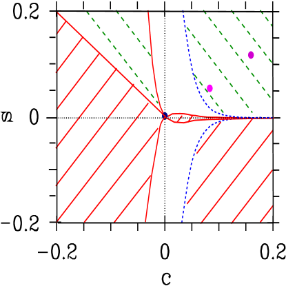
Figure 1: The theoretically expected region for the parameters $s$ and $c$ for a value of $N_{\rm 0}=50$; the solid(red)-line-hatched region is strongly excluded, while the dashed(green)-line-hatched region is excluded only if the mass is supposed to run up to the end of inflation. The dotted (blue) line gives the prediction for the case when the end of inflation is triggered by $\eta=1$. The circles correspond to the values in the explicit models discussed in section II.C: the upper ones (magenta) refer to the case of gauge coupling dominance, while the (blue) one at the origin to the case of Yukawa coupling dominance.

Since $\epsilon$ is negligible, the spectral index to second order is

$$n(k) = 1+2\eta\left(1+{\eta\over 3}\right)+2.13\,\xi^{2}\,.$$ (28)

This gives cl98

$${n(k)-1\over 2} = se^{c\Delta N(k)}\left(1-1.06c\right)-c$$ (29)

$$+{1\over 3}\left(se^{c\Delta N(k)}-c\right)^{2}\,.$$

The first derivative of the spectral index is given by

$$n^{\prime}(k)\equiv\frac{\mbox{d}n(k)}{\mbox{d}\ln k}=2sc\,e^{c\Delta N(k)}\,.$$ (30)

Clearly the spectral index is not constant within cosmological scales unless $s$ or $c$ is very close to zero. Note that for this type of models, $n^{\prime}$ is a higher order effect (suppressed by both $c$ and $s$) as in usual slow-roll inflation, but it is not proportional to $(n-1)^{2}$. So it is perfectly allowed to have $n=1$ at a particular scale, with a non-zero running. This is again a consequence of our initial assumption that in the region of the potential where inflation takes place the one-loop contribution to the inflaton mass is of the same order as the tree one. Note anyway that the perturbative expansion is not endangered by our assumption, since the higher orders stay always smaller than the one-loop. Similarly for the slow-roll expansion, the second order can become larger than the first one in case of strong cancellation between $s$ and $c$, but the perturbative expansion is still solid.

At the pivot scale, we have, for example, to second order in $s,c$

$$n_{\rm 0}-1 = 2(s-c-1.06sc)+{2\over 3}(s-c)^{2}$$ (31)

$$n^{\prime}_{\rm 0} = 2sc\,.$$ (32)

The line $s=c/(1-1.06c)$ in the $s$ vs $c$ plane corresponds approximately to $n_{\rm 0}=1$. The Harrison-Zeldovich case of constant $n=1$ is given by the origin $s=c=0$, while constant spectral index different from $1$ is realized either near the $c=0$ axis for $s=(n-1)/2$ or near the $s=0$ axis for $c=-(n-1)/2$.

Since the phenomenological parameters only depend on $s-c$ and $sc$, as long as higher orders are negligible, the allowed region is expected to be symmetric under reflection along the $s+c=0$ line. We can solve the system of equations exactly and extract the parameters $s$ and $c$ from a measurement of $n_{\rm 0}$ and $n^{\prime}_{\rm 0}$; one solution is given as

$$c_{1} = -{1\over 4}\left[n_{\rm 0}-1+1.06n^{\prime}_{\rm 0}\right.$$

$$\left.-\sqrt{\left(n_{\rm 0}-1+1.06n^{\prime}_{\rm 0}\right)^{2}+8n^{\prime}_{\rm 0}}\right].$$

$$s_{1} = {1\over 4}\left[n_{\rm 0}-1+1.06n^{\prime}_{\rm 0}\right.$$

$$\left.+\sqrt{\left(n_{\rm 0}-1+1.06n^{\prime}_{\rm 0}\right)^{2}+8n^{\prime}_{\rm 0}}\right]\;.$$

the second solution is given just by the symmetry, i.e. $c_{2}=-s_{1}$ and $s_{2}=-c_{1}$.

From the expressions above, it is clear that not all values of $n^{\prime}_{\rm 0}$ are allowed in the running mass model: we obtain the constraint

$$n^{\prime}_{\rm 0}\geq-{(n_{\rm 0}-1)^{2}\over 4}\,,$$ (35)

so that a decreasing spectral index is possible only if $n_{\rm 0}$ is different from 1. So in general the prediction of the running mass model tends toward positive $n^{\prime}$, contrary to the result claimed by WMAP WMAP-peiris . Both due to this constraint and the exponential dependence on $c$, we see that fitting for arbitrary value of $n^{\prime}$ is not equivalent to performing a fit for the running mass model. Note also that, as discussed in clm03 , the fact that the running mass model tends in general to give more power at low scales for sufficiently large $c$, can give naturally a large value of the reionization redshift in the Press-Schechter approximation and accommodate easily the value obtained by WMAP spergel .

We will show in the following the allowed region both in the $s,c$ parameter space and in the $n^{\prime}_{\rm 0}$ vs $n_{\rm 0}-1$ plane.

II.3 Explicit minimal models

1. Dominance of the gauge interaction

The first model to be proposed st97 ; st97bis considered the case of an inflaton charged under an asymptotically free $SU(N)$ group. We will consider the case of two matter superfields in the adjoint representation as in c98 , where one has very simply a superpotential given by

$$W=gS\,{\rm Tr}\,\left(\phi_{1}\phi_{2}\right)\;,$$ (36)

then e.g. the direction $\phi=\phi_{1}^{1}$ is D- and F-flat for vanishing other fields. Note that here for the case of universal SUSY breaking masses, the role of the waterfall field can be played by the singlet $S$ c98 and the gauge symmetry is unbroken in the true vacuum.

We can then write easily the $\beta$-functions,

$$\beta_{m}=-{2N\over\pi}\alpha\tilde{m}^{2}\;\quad\quad\tilde{m}\propto\alpha\,,$$ (37)

while for the gauge coupling

$${d\alpha\over d\ln Q}=-{N\over 2\pi}\alpha^{2}\,,$$ (38)

giving

$$\alpha(\ln\phi)={\alpha(M_{\rm P})\over 1+{N\alpha_{0}\over 2\pi}\ln\phi}.$$ (39)

So the RG equation for the soft mass can be solved analytically to give

$$m_{\phi}^{2}\left(\ln\phi\right) = m_{\phi}^{2}(M_{\rm P})-2\tilde{m}^{2}(M_{\rm P})$$ (40)

$$+{2\tilde{m}^{2}(M_{\rm P})\over(1+{N\over 2\pi}\alpha(M_{\rm P})\ln\phi)^{2}}\;,$$

where we have defined the boundary conditions at $M_{\rm P}$ .

It is then clear that the inflaton mass increases for decreasing $\phi<M_{\rm P}$ and therefore to obtain a reduction of the mass absolute value a negative initial mass is necessary.

For the linear approximation, we have then

$$c = {2N\over\pi}\alpha\left(\ln\phi_{0}\right)\;{\tilde{m}^{2}(\ln\phi_{0})\over 3H_{I}^{2}}$$ (41)

$$= {2N\alpha(M_{\rm P})\over\pi}{\tilde{m}^{2}(M_{\rm P})\over 3H_{I}^{2}}{\alpha^{3}(\ln\phi_{0})\over\alpha^{3}(M_{\rm P})}\,;$$ (42)

which is a positive number, and

$$s+{1\over 2}c = {m_{\phi}^{2}(\ln\phi_{0})\over 3H_{I}^{2}}$$ (44)

$$= {m_{\phi}^{2}(M_{\rm P})-2\tilde{m}^{2}(M_{\rm P})\over 3H_{I}^{2}}$$

$$+{2\tilde{m}^{2}(M_{\rm P})\over 3H_{I}^{2}}\;{\alpha^{2}(\ln\phi_{0})\over\alpha^{2}(M_{\rm P})}$$

so $s$ can be positive or negative.

The power spectrum normalization gives us instead:

$$\ln\left(\phi_{0}\right)+\ln(2\pi|s|)=\ln\left({\cal P}_{{\cal R}}^{1/2}(k_{\rm 0})H_{I}\right).$$ (45)

The expression above can provide directly an estimate of the order of magnitude of $\phi_{0}$, but unfortunately it is not possible to solve directly for this quantity. We can instead turn the formula around and use it to define the inflationary scale, after we have singled out the region where the spectral index is small.

For $\phi_{0}$ we can use as a very rough estimate instead the scale where $m^{2}_{\phi}$ exactly vanishes, $\phi_{m=0}$:

$$\ln\left(\phi_{m=0}\right)\simeq{-2\pi\over N\alpha(M_{\rm P})}\left[1-\left(1+{|m^{2}_{\phi}(M_{\rm P})|\over 2\tilde{m}^{2}(M_{\rm P})}\right)^{-1/2}\right];$$ (46)

depending on the value of the coupling constant, the scale $\phi_{m=0}$ changes very strongly. Note that in order for $n_{\rm 0}$ to be phenomenologically acceptable, $\phi_{0}$ must be not much far away: the value of the spectral index at $m^{2}_{\phi}=0$ is in fact already small,

$$n_{m=0}-1\simeq-3c\;.$$ (47)

Assuming $\alpha(M_{\rm P})\simeq 1/24$ as in SUSY-GUT models, $N=3$ and $|m_{\phi}^{2}(M_{\rm P})|=\tilde{m}^{2}(M_{\rm P})=3H_{I}^{2}$, we obtain for example

$$\phi_{m=0}=9.9\times 10^{-5}M_{\rm P}\,;$$ (48)

so that the inflationary scale must therefore be

$$H_{I}\sim 10^{-9}M_{\rm P}\sim 10^{9}\,\mbox{GeV}.$$ (49)

For the parameters $c,s$ at that point we obtain the values:

$$c_{m=0} \simeq 0.15$$ (50)

$$s_{m=0} \simeq -0.07$$ (51)

as expected. This corresponds to

$$n(k_{m=0})-1=-0.44$$ (52)

too large to be phenomenologically acceptable, but e.g for $\phi_{0}=0.25\,\phi_{m=0}$ one has

$$c \simeq 0.16$$ (53)

$$s \simeq 0.13$$ (54)

and therefore

$$n(k_{0})-1 = -0.06$$ (55)

$$n^{\prime}(k_{0}) = 0.04\;.$$ (56)

We see clearly that the spectral index can be very small, but with a running of the same order.

Note anyway that changing $\alpha(M_{\rm P})$ by only a factor $1/2$, we obtain much smaller values:

$$\phi_{m=0}=9.74\times 10^{-9}M_{\rm P}\,;$$ (57)

so that the inflationary scale must therefore be

$$H_{I}\sim 10^{-13}M_{\rm P}\sim 10^{5}\,\mbox{GeV}.$$ (58)

This strong dependence on the coupling is characteristic of dimensional transmutation and allows us to construct viable models spanning a very large range of $H_{I}$, while presenting similar values for the spectral index and its running. It is therefore possible to accommodate practically all the scales in eq. 12, and in general smaller $H_{I}$ corresponds to smaller gauge coupling, which for the same gaugino mass means smaller $c$. In fact in this case we have at $\phi_{0}=\;0.25\phi_{m=0}$:

$$c \simeq 0.08$$ (59)

$$s \simeq 0.06$$ (60)

and therefore

$$n(k_{0})-1 = -0.02$$ (61)

$$n^{\prime}(k_{0}) = 0.01\;.$$ (62)

2. Dominance of the Yukawa coupling

We consider here the simplest of the cases studied in c98 , where the superpotential is given by

$$W=\lambda\phi_{1}\phi_{2}\phi_{3}$$ (63)

and all fields are singlet under gauge interaction. If the trilinear susy breaking coupling vanishes, we have:

$${d\lambda\over d\ln Q} = {3\lambda\over 16\pi^{2}}|\lambda|^{2}$$ (64)

$${dm_{i}^{2}\over d\ln Q} = {|\lambda|^{2}\over 8\pi^{2}}\sum_{j}m_{j}^{2}\;.$$ (65)

Then for the average scalar mass $\bar{m}^{2}=\sum_{i}m_{i}^{2}/3$, we obtain the simple expression:

$$\bar{m}^{2}(\ln\phi/M_{\rm P})={\bar{m}^{2}(M_{\rm P})\over 1-{3\over 8\pi^{2}}\lambda^{2}(M_{\rm P})\ln\phi}\;.$$ (66)

The mass differences instead are constant, so for the single masses we have:

$$m_{i}^{2}(\ln\phi)=\bar{m}^{2}(\ln\phi)-\bar{m}^{2}(M_{\rm P})+m^{2}_{i}(M_{\rm P})\;.$$ (67)

Note that in this case the masses run from positive to negative and that the running is strong at the beginning and then tends to flatten out at the value given by $\bar{m}^{2}=0$. In fact in this case the Yukawa is non-asymptotically free and tends to zero at small scales. So in the plateau region, if $m^{2}(M_{\rm P})\simeq\bar{m}^{2}(M_{\rm P})$, we have automatically a flat potential.

In this specific model, slow roll inflation can be realized in any of the 3 field directions, but we have to consider some non-universal initial masses, since the hybrid end is assured only if one of them becomes negative, but not all at the same time. For example assume $\phi_{1}$ to be the inflaton and some non-universal mass terms coming from higher order term in the Kähler potential so that $m_{1}^{2}(M_{\rm P})=H_{I}^{2}$, but $m_{2}^{2}(M_{\rm P})+m_{3}^{2}(M_{\rm P})=5H_{I}^{2}$. Then we have for the inflaton mass

$$m^{2}(\ln\phi)={2H_{I}^{2}\over 1-{3\over 8\pi^{2}}\lambda^{2}(M_{\rm P})\ln\phi}-H_{I}^{2}$$ (68)

and in the linear approximation this gives

$$c = -\frac{\lambda^{2}(\phi_{0})\,\bar{m}^{2}(\phi_{0})}{8\pi^{2}\,H_{I}^{2}}$$ (69)

$$= -\frac{\lambda^{2}(M_{\rm P})}{12\pi^{2}}{1\over\left(1-{3\over 8\pi^{2}}\lambda^{2}(M_{\rm P})\ln\phi_{0}\right)^{2}}$$

$$s = -\frac{c}{2}+\frac{2}{3}\left[{1\over 1-{3\over 8\pi^{2}}\lambda^{2}(M_{\rm P})\ln\phi_{0}}-\frac{1}{2}\right]\;;$$

so that $c$ is negative, while $s$ can have either sign. We note that in this type of models, the parameter $c$ is related to second power of the coupling constant and therefore $\lambda$ has to be sufficiently large to give an effect.

As long as $s$ does not vanish in the interesting region, we can find an estimate of $\phi_{0}$ from the COBE normalization. Since the running is slower in this case, we can solve iteratively eq. (45) for $\phi_{\rm 0}$ and $s$, taking $H_{I}=10^{-15}M_{\rm P}\sim 10^{3}\,\mbox{GeV}$ and $\lambda(M_{\rm P})=1$. We obtain then

$${\phi_{\rm 0}\over M_{\rm P}}=1.3\times 10^{-10}$$ (71)

and

$$c = -0.002$$ (72)

$$s = 0.026\;.$$ (73)

We can in this case have $|c|<0.01$ since we have assumed a somewhat suppressed initial inflaton mass $m^{2}(M_{\rm P})=H_{I}^{2}<3H_{I}^{2}$. So in this case we have very small scale dependence:

$$n(k_{\rm 0})-1 = 0.056$$ (74)

$$n^{\prime}(k_{\rm 0}) = -0.0001.$$ (75)

III Observational constraints

III.1 Method

Our analysis method is based on the computation of a likelihood distribution over a grid of precomputed theoretical models.

We restrict our analysis to a flat, adiabatic, $\Lambda$-CDM model template computed with a modified version of CMBFAST CMBFAST , sampling the parameters as follows: $\Omega_{cdm}h^{2}\equiv\omega_{cdm}=0.05,...0.20$, in steps of $0.01$; $\Omega_{b}h^{2}\equiv\omega_{b}=0.0018,...,0.030$, in steps of $0.001$ and $h=0.55,...,0.85$, in steps of $0.05$. The value of the cosmological constant $\Lambda$ is determined by the flatness condition. Our choice of the above parameters is motivated by Big Bang Nucleosynthesis bounds on $\omega_{b}$ (both from $D$ burles and ${}^{4}He+^{7}Li$ cyburt ), from supernovae super1 and galaxy clustering observations (see e.g. thx ). Current data also does not show evidence for additional physics like quintessence (see e.g. bean ), extra-relativistic particles (see e.g. bowen ), topological defects (see e.g. dkm ) or isocurvature perturbations (see e.g. jxd ). We do not consider massive neutrino which may have an effect on our results but that are probably negligible (see e.g. fogli ). From the grid above we only consider models with age of the universe $t_{0}>11$ Gyrs. We allow for a possible (instantaneous) reionization of the intergalactic medium by varying the reionization redshift $5<z_{ri}<25$ and we allow a free re-scaling of the fluctuation amplitude by a pre-factor of the order of $C_{110}$, in units of $C_{110}^{WMAP}$ as measured by the WMAP satellite. Finally, we let the running parameters $c$ and $s$ vary as follows: $-0.2<c<0.2$, and $-0.2<s<0.2$ in steps of $0.008$.

The theoretical models are compared with the recent temperature and temperature-polarization WMAP data using the publicly available likelihood code WMAPanalysis03 .

In addition to the CMB data we also consider the constraints on the real-space power spectrum of galaxies from the SLOAN galaxy redshift surveys using the data and window functions of the analysis of  Tg04 . We restrict the analysis to a range of scales over which the fluctuations are assumed to be in the linear regime ($k<0.2h^{-1}\rm Mpc$). When combining with the CMB data, we marginalize over a bias $b$ considered as an additional free parameter.

We also include information from the Lyman-alpha Forest in the Sloan Digital Sky Survey using the results of the analysis of Se04 and Mc04 which probes the amplitude of linear fluctuations at very small scales. For this dataset, small-scale power spectra are computed at high redshifts and compared with the values presented in Mc04 .

III.2 Results

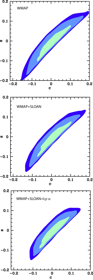
Figure 2: Likelihood contour plot in the $c-s$ plane showing the $1$,$2$ and $3\sigma$ contours from the WMAP data (Top Panel), WMAP+SLOAN (Middle Panel) and WMAP+SLOAN+Ly-$\alpha$ (Bottom Panel).

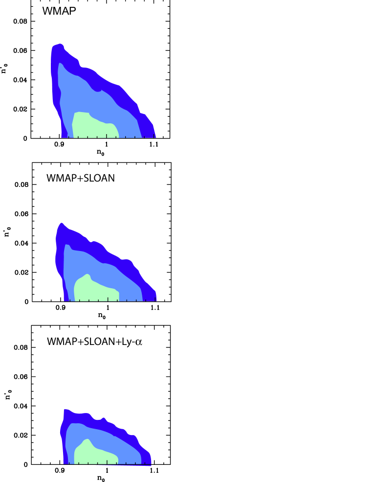
Figure 3: Likelihood contour plot in the $n_{\rm 0}-n^{\prime}_{\rm 0}$ plane showing the $1$,$2$ and $3\sigma$ contours from the WMAP data (Top Panel), WMAP+SLOAN (Middle Panel) and WMAP+SLOAN+Ly-$\alpha$ (Bottom Panel).

Figure 4: Likelihood contour plot in the plane $c-(s+c/2)$ showing the $1$,$2$ and $3\sigma$ contours from the WMAP+SLOAN+Ly-$\alpha$ data. We recall that these parameters are related to the physical inflaton potential parameters by $c=-\beta_{m}(\ln\phi_{0})/(3H_{I}^{2})$ and $s+c/2=m^{2}(\ln\phi_{0})/(3H_{I}^{2})$.

In Fig. 2 we plot the likelihood contours in the $c-s$ plane showing the $1$, $2$ and $3\sigma$ contours. The top panel is WMAP, middle WMAP+SLOAN and bottom panel WMAP+SLOAN+Ly-$\alpha$. As we can see there is a strong correlation between the two parameters along the $c-s$ direction and the inclusion of the SLOAN data does not improve significantly the CMB constraints. However adding the Lyman-$\alpha$ datasets breaks the degeneracy and shrinks the likelihoods. As already noticed by Se04 , we find that the Lyman $\alpha$ data are able to restrict more strongly the scale dependence of the spectral index and therefore exclude the parameter space at large $|c|$; in particular at $68\%$ we have $sc<0.0043$.

Focusing on the region ($s+c>0$), we plot the likelihood contours in the $2(s-c)+1$ vs. $2sc$ plane in Figure 3. As we explained before, $2(s-c)+1$ gives the value of the spectral index $n_{0}$, while $2sc=n^{\prime}_{0}$ gives the bend in the spectrum. Note that due to the bound (35), the viable negative running region is practically indistinguishable from the $n_{0}^{\prime}=0$ axis in our scale and therefore we do not show it. The maximal negative running is in fact $-0.0015$ at $95\%$ c.l. and it does not basically change with the different datasets. As we can see from the figure, the WMAP data alone constrains $n^{\prime}_{\rm 0}<0.05$ at $95\%$ C.L.. Including the constraints from SLOAN and Ly-$\alpha$ limits the amount of deviation from scale invariance to $n^{\prime}_{\rm 0}<0.024$ at $95\%$ c.l..

Finally, in Fig.4 we plot the likelihood contours in the $c$ vs. $s+c/2$ plane. As discussed previously, this variables correspond to the physical parameters in the inflaton potential rescaled by the inflationary scale $3H_{I}^{2}$. It is clear from the graph that the data require a correlation between the inflaton mass and the $\beta$-function for large $c$ in order to give a small $n_{0}-1$. It is questionable if such correlation corresponds to a fine-tuning, and in general depends on the explicit realization of the model. In fact in the gauge dominated case, we have already emphasized that there is relatively large freedom, since the physical parameters are more than the observables. For the Yukawa dominated case the situation is more constraint, also because the running is weaker and to be effective requires always large couplings. In Figure 1 are shown the three points in the parameter space that we looked at in detail in Section III C. We see that WMAP+SLOAN datasets are not able to exclude any of the models, but the inclusion of Ly-$\alpha$ excludes the first model discussed at $99\%$ c.l..

IV Conclusions

The rather full analysis that we have described confirms the general picture indicated by previous analysis covi ; clm03 . The allowed region in the $c$ vs $s$ plane depicted in Figure 2 should be compared with the region shown in Figure 1 which approximately delineates the theoretically disfavoured region, and also with the minimum value $|c|\sim 10^{-2}$ which is probably needed to generate enough running of the mass even if we go from the Planck scale to $100\,\mbox{GeV}$. Combining all of these, we see that if $|c|$ is significantly above the minimum value, only the version of the model with $c$ and $s$ both positive is viable. In that case, the spectral index has significant running which will be detectable in the foreseeable future. On the other hand, if $|c|$ is really of order $10^{-2}$, all choices of the signs of $c$ and $s$ are possible except maybe negative $c$ with positive $s$. Furthermore, if that extreme case can be realized in a viable running-mass model the running of $n$ will be so small that it may never be detectable. The data are now starting to squeeze the allowed region to values $|c|\leq 0.1$, still away from the lower bound $10^{-2}$. The smallness of $|c|$ could be interpreted as a hint that the inflationary scale needs probably to be low, to make the running from $M_{\rm P}$ effective. Note anyway that $H_{I}$ values of the order of $100\,\mbox{GeV}$, the expected soft SUSY breaking masses in the true vacuum from gravity mediation, are still acceptable, as demonstrated in the cases of the simple models presented.

Looking at the observational situation in more detail, our results show again that the CMB data can put very strong constraints on the value of the spectral index at large scales, $n_{0}=1+2(s-c)$, but still allow a pretty large scale-dependence. Other information on the power spectrum, like Lyman $\alpha$ data, are needed to reduce the parameter space in the orthogonal direction. Even with this inclusion, though, values of $|c|$ of the order of 0.1 are allowed and we have $n^{\prime}_{\rm 0}\leq 0.037$ at $99\%$ c.l.. Our allowed region also looks still symmetric under reflection with respect to the $s+c=0$ line: this means that the present data are not sensitive enough to distinguish the variation of $n^{\prime}$ that is predicted by the running-mass model.

Acknowledgments

LC would like to thank D. Schwarz and C. Scrucca for useful discussions. CJO is supported by a Marie Curie Intra-European Fellowship, grant $501007$.

References

- (1) C.L. Bennett et al., Astrophys. J. Suppl. 148 (2003) 1 [arXiv:astro-ph/0302207].
- (2) D. N. Spergel et al., Astrophys. J. Suppl. 148 (2003) 175 [arXiv:astro-ph/0302209].
- (3) A. Melchiorri and C. Odman, arXiv:astro-ph/0302361.
- (4) SDSS Collaboration, M. Tegmark et al., Phys. Rev. D69 (2004) 103501 [arXiv:astro-ph/0310723].
- (5) U. Seljak et al., arXiv:astro-ph/0407372.
- (6) D. H. Lyth and D. Wands, Phys. Lett. B524, 5 (2002) [arXiv:hep-ph/0110002]; T. Moroi and T. Takahashi, Phys. Lett. B522 (2001) 215 [arXive:hep-ph/0110096] and Phys. Rev. D66 (2002) 063501 [arXive:hep-ph/0206026].
- (7) S. Mollerach, Phys. Rev. D42 (1990) 313; A. D. Linde and V. Mukhanov, Phys. Rev. D56 (1997) 535 [arXive:astro-ph/9610219].
- (8) H. V. Peiris et al., Astrophys. J. Suppl. 148 (2003) 213 [arXiv:astro-ph/0302225].
- (9) W. H. Kinney, E. W. Kolb, A. Melchiorri and A. Riotto, Phys. Rev. D69 (2004) 103516 [arXiv:hep-ph/0305130].
- (10) S. M. Leach and A. R. Liddle, Phys. Rev. D68 (2003) 123508 [arXiv:astro-ph/0306305].
- (11) D. H. Lyth and A. Riotto, Phys. Rept. 314 (1999) 1 [arXiv:hep-ph/9807278].
- (12) A. R. Liddle and D. H. Lyth, “Cosmological Inflation And Large-Scale Structure,” Cambridge, UK: Univ. Pr. (2000) 400 p.
- (13) E. D. Stewart, Phys. Lett. B391 (1997) 34 [arXiv:hep-ph/9606241].
- (14) E. D. Stewart, Phys. Rev. D56 (1997) 2019 [arXiv:hep-ph/9703232].
- (15) L. Covi, D. H. Lyth and L. Roszkowski, Phys. Rev. D60 (1999) 023509 [arXiv:hep-ph/9809310].
- (16) L. Covi and D. H. Lyth Phys. Rev. D59 (1999) 063515 [arXiv:hep-ph/9809562].
- (17) L. Covi Phys. Rev. D60 (1999) 023513 [arXiv:hep-ph/9812232].
- (18) G. German, G. Ross and S. Sarkar, Phys. Lett. B469 (1999) 46 [arXiv: hep-ph/9908380].
- (19) U. Seljak, P. McDonald and A. Makarov, Mon. Not. Roy. Astron. Soc. 342 (2003) L79 [arXiv:astro-ph/0302571]; M. Viel, J. Weller and M. G. Haehnelt, arXiv:astro-ph/0407294.
- (20) L. Covi, D. H. Lyth and A. Melchiorri Phys. Rev. D67 (2003) 043507 [arXiv:hep-ph/0210395].
- (21) W. Buchmüller, L. Covi and D. Delépine, Phys. Lett. B491 (2000) 183 [arXiv:hep-ph/0006168].
- (22) A. D. Linde, Phys. Lett. B259 (1991) 38.
- (23) L. Randall, M. Soljacic and A. H. Guth, Nucl. Phys. B 472 (1996) 377 [arXiv:hep-ph/9512439].
- (24) M. Zaldarriaga & U. Seljak, Astrophys. J. 469 (1996) 437 [arXiv:astro-ph/9603033].
- (25) S. Burles, K. M. Nollett and M. S. Turner,Astrophys. J. 552 (2001) L1 [arXiv:astro-ph/0010171].
- (26) R. H. Cyburt, B. D. Fields and K. A. Olive, New Astron. 6 (1996) 215 [arXiv:astro-ph/0102179].
- (27) P.M. Garnavich et al, Astrophys. J. Letters 493 (1998) L53 [arXiv:astro-ph/9710123]; S. Perlmutter et al, Astrophys. J. 483 (1997) 565 [arXiv:astro-ph/9608192]; S. Perlmutter et al (The SupernovaCosmology Project), Nature 391 (1998) 51 [arXiv:astro-ph/9712212]; A.G. Riess et al, Astron. J. 116 (1998) 1009 [arXiv:astro-ph/9805201].
- (28) M. Tegmark, A. J. S. Hamilton and Y. Xu, Mon. Not. Roy. Astron. Soc. 335 (2002) 887 [arXiv:astro-ph/0111575].
- (29) R. Bean and A. Melchiorri, Phys. Rev. D65 041302 (2002) [arXiv:astro-ph/0110472].
- (30) R. Bowen, et al. Mon. Not. Roy. Astron. Soc. 334 (2002) 760 [arXiv:astro-ph/0110636].
- (31) R. Durrer, et al. Phys. Rev. D 59 (1999) 123005 [arXiv:astro-ph/9811174].
- (32) J. Dunkley, M. Bucher, P. G. Ferreira, K. Moodley and C. Skordis, arXiv:astro-ph/0405462.
- (33) G. L. Fogli, et al. arXiv:hep-ph/0408045.
- (34) L. Verde et al., Astrophys. J. Suppl. 148 (2003) 195 [arXiv:astro-ph/0302218]; G. Hinshaw et al., Astrophys. J. Suppl. 148 (2003) 135 [arXiv:astro-ph/0302217].
- (35) SDSS Collaboration, P. McDonald et al., arXiv:astro-ph/0405013.
- (36) D. H. Lyth and L. Covi, Phys. Rev. D62 (2000) 103504 [arXiv:astro-ph/0002397]; L. Covi and D. H. Lyth, Mon. Not. Roy. Astron. Soc. 326 (2001) 885 [arXiv:astro-ph/0008165].