Metallicities of $0.3<z<1.0$ Galaxies in the GOODS-North Field

Abstract

We measure nebular oxygen abundances for 204 emission-line galaxies with redshifts $0.3<z<1.0$ in the Great Observatories Origins Deep Survey North (GOODS-N) field using spectra from the Team Keck Redshift Survey (TKRS). We also provide an updated analytic prescription for estimating oxygen abundances using the traditional strong emission line ratio, $R_{23}$, based on the photoionization models of Kewley & Dopita (2003). We include an analytic formula for very crude metallicity estimates using the $[N~{}II]_{\lambda 6584}/H\alpha$ ratio. Oxygen abundances for GOODS-N galaxies range from $8.2\leq 12+\log(O/H)<9.1$ corresponding to metallicities between 0.3 and 2.5 times the solar value. This sample of galaxies exhibits a correlation between rest-frame blue luminosity and gas-phase metallicity (i.e., an L-Z relation), consistent with L-Z correlations of previously-studied intermediate-redshift samples. The zero point of the L-Z relation evolves with redshift in the sense that galaxies of a given luminosity become more metal poor at higher redshift. Galaxies in luminosity bins $-18.5<M_{B}<-21.5$ exhibit a decrease in average oxygen abundance by 0.14$\pm 0.05$ dex from $z=0$ to $z=1$. This rate of metal enrichment means that $28\pm 0.07$% of metals in local galaxies have been synthesized since $z=1$, in reasonable agreement with the predictions based on published star formation rate densities which show that $\sim 38$% of stars in the universe have formed during the same interval. The slope of the L-Z relation may evolve in the sense that the least luminous galaxies at each redshift interval become increasingly metal poor compared to more luminous galaxies. We interpret this change in slope as evidence for more rapid chemical evolution among the least luminous galaxies ($M_{B}>-20$), consistent with scenarios whereby the the formation epoch for less massive galaxies is more recent than for massive galaxies.

1 Metallicity in Galaxy Evolution and Modeling

The chemical composition of galaxies is fundamentally important for tracing galaxy evolution and for modeling galaxy properties. Galaxy evolution prescriptions dating from Tinsley (1974, 1980) to present computational codes (e.g., STARBURST99 – Leitherer et al. 1999; Bruzual & Charlot 2003; Pégase – Fioc, M. & Rocca-Volmerange 1999; GRASIL – Silva et al. 1998) incorporate metallicity as a primary ingredient in tracking a galaxy’s growth. Metallicity determines a galaxy’s UV and optical colors at a given age, the strength of stellar and interstellar metallic absorption lines, the shape of its interstellar extinction curve (e.g., Prévot et al. 1984), its dust to gas ratio (Dwek 1998; Issa, MacLaren, & Wolfendale 1990), its nucleosynthetic yields (e.g., Woosley & Weaver 1995), and perhaps even its rate of star formation (Nishi & Tashiro 2000). Overall metal abundance and elemental abundance ratios trace the star formation history and nucleosynthetic history of a galaxy (reviewed by Wheeler, Sneden & Truran 1989). These abundances and ratios also reflect the importance of gas inflow and outflow in a galaxy’s evolution (galactic winds–Matthews & Baker 1971; metal-rich galactic winds–Vader 1987) . Observational studies have now begun to provide detailed optical and infrared measurements of thousands of galaxies at redshifts from 0.1 to 6 (e.g., Rowan-Robinson et al. 2001; Hippelein et al. 2003; Sullivan et al. 2004; van Dokkum et al. 2004; Steidel et al. 2004, and references therein), spanning the vast majority of cosmic time. Successful modeling of the evolutionary paths of these galaxies will require, among other parameters, secure measurements of their chemical compositions.

Direct measurements of metallicities in distant galaxies are now becoming routine, spurred on by larger telescopes and more capable spectrographs used in deep galaxy surveys. Kobulnicky & Zaritsky (1999) first applied classical nebular diagnostic techniques developed for H II regions in local galaxies to the global spectra of 14 compact star-forming galaxies at $0.1<z<0.5$. Their sample spanned a range of galaxy luminosities from $-17>M_{B}>-22$ and oxygen abundances from $8.25<12+log(O/H)<9.02$. Carollo & Lilly (2001) presented oxygen abundances for 15 luminous galaxies from the Canada-France Redshift Survey (CFRS; Lilly et al. 1995) over the range $0.60<z<0.98$ and $-20.1>M_{B}>-22.6$. Both of these early works concluded that intermediate redshift galaxies were consistent with the same correlation between luminosity and metallicity (i.e., the L-Z relation) observed in local samples (e.g., Faber 1973; Lequeux et al. 1979; Skillman, Kennicutt, & Hodge 1989; Zaritsky, Kennicutt, & Huchra 1994, hereafter ZKH). Meanwhile, Kobulnicky & Koo (2000), Pettini et al. (2001), and Shapley et al. (2004) used near-infrared spectroscopy of $2.1<z<3.5$ Lyman break galaxies to measure gas-phase oxygen abundances. These authors concluded that the high redshift objects were 2-4 magnitudes more luminous than $z=0$ galaxies with comparable $8.3<12+log(O/H)<9$ metallicities and thus were inconsistent with the local L-Z relation. Evidence for evolution of the L-Z relation with epoch, particularly among sub L* galaxies with $M_{B}$ fainter than $-20$, grew with metallicity measurements of 64 $0.26<z<0.82$ field galaxies in the Groth Strip Survey (DGSS–Kobulnicky et al. 2003; Ke03) and 66 additional CFRS galaxies at $0.47<z<0.92$ (Lilly, Carollo & Stockton 2003–LCS03; Carollo & Lilly, 2001–CL01). Recently, Maier, Meisenheimer & Hippelein (2004) measured metallicities for 5 sub L* galaxies at $z\sim 0.4$ and 10 sub L* galaxies at $z\sim 0.64$ from the CADIS emission-line survey. These additional sub L* galaxies provide further support for the evolution of the L-Z relation with epoch.

In this paper we present gas-phase oxygen abundance measurements for 204 emission-line galaxies from $0.3<z<0.93$ in the Great Observatories Origins Deep Survey-North (GOODS-North; Dickinson et al. 2001) field using the publicly available spectra obtained as part of the Team Keck Treasury Redshift Survey (TKRS; Wirth et al. 2004). The new data double the number of metallicities previously available for this redshift range and constitute the highest quality spectra yet available for chemical analysis. In addition to providing new constraints on the chemical enrichment of galaxies over the last 8 Gyr, it is our hope that these measurements will prove useful for the community in modeling the evolution of galaxies in this well-studied cosmological field. We combine these new TKRS data with existing emission line measurements from the literature (CFRS–LCS03 ; DGSS–Kobulnicky et al. 2003) to assess the chemo-luminous evolution of star-forming galaxies out to $z=1$. Where applicable, we adopt a cosmology with $H_{0}$=70  km s^-1 Mpc^-1, $\Omega_{m}=0.3$, and $\Omega_{\Lambda}=0.7$.

2 Data Analysis

2.1 Target Selection

The TKRS consists of Keck telescope spectroscopy with the DEIMOS (Faber et al. 2003) spectrograph over the nominal wavelength range 4600 Å – 9800 Å. Targets include both stars and galaxies, selected in an unbiased manner from all objects with $R\leq 24.4$ in ground-based optical images (Wirth et al. 2004). Slitmasks with 1^′′ wide slits tilted to align with a galaxy’s major axis provided up to 100 spectra per 1200 s exposure. Spectra have typical resolutions of $\sim$3.5 Å and total integration times of 3600 s.

We searched the publicly available TKRS spectroscopic database for galaxies with nebular emission lines suitable for chemical analysis. Only galaxies where it was possible to measure all of the requisite [O II]$\lambda 3727$, H$\beta$, and [O III]$\lambda$5007 lines were retained. These criteria necessarily exclude objects at redshifts of $z\lesssim 0.3$ since the requisite [O II]$\lambda$3727 line falls below the blue limit of the spectroscopic setup. Likewise, objects with redshifts $z\gtrsim 1.0$ are excluded because the [O III]$\lambda$5007 line falls beyond the red wavelength limit of the survey. In the 2004 February public release of the TKRS there were 1536 objects with secure redshifts. Of these, 1044 fell within our redshift limits. Of the 1044 candidates, 497 were removed from consideration because no emission lines were present in the spectrum. Next, 94 galaxies were removed from the sample because one of the requisite strong emission lines fell off the end of the wavelength coverage (or in between the red and blue spectral regions) due to the object’s placement on the slitmask. Following Kobulnicky et al. 2003), we removed 94 objects in the redshift ranges $0.410<z<0.426$, $0.52<z<0.54$, and $0.56<z<0.58$. For these intervals, atmospheric $O_{2}$ absorption troughs between 6865 Å – 6920 Å (the “B band”) and between 7585 Å – $\sim 7680$ Å (the “A band”) prohibit accurate measurement of emission lines. Another 122 objects were removed from the sample because the $H\beta$ emission line was absent or too weak (S/N$<$8:1) for reliable chemical determinations (see Kobulnicky, Kennicutt, & Pizagno 1999 for a discussion of errors and uncertainties). The spectra of objects rejected due to a weak $H\beta$ line are usually dominated by stellar continuum rather than nebular emission from star-forming regions. Most local early-type spirals and elliptical galaxies share these spectral characteristics. For these objects, H$\beta$ is seen in absorption against the stellar spectrum of the galaxy. Thus early type galaxies with older stellar populations are preferentially rejected in favor of late type galaxies with larger star formation rates. An additional 31 galaxies had to be rejected because some combination of strong night sky emission bands, low continuum, or poor continuum subtraction caused the extracted 1-D spectrum to have continuum levels that were either negative or very close to zero. Because chemical analysis requires emission lines powered by normal stellar ionizing radiation fields (as opposed to nonthermal sources from active galactic nuclei), we rejected 9 objects exhibiting canonical AGN or LINER signatures: broad emission lines (2 objects), or $EW_{[Ne~{}III]\lambda 3826}/EW_{[O~{}II]\lambda 3727}$ ratios exceeding 0.4 (7 objects) (e.g., Osterbrock 1989). The resulting usable sample contained 204 emission-line galaxies.

Twenty-seven of the 204 selected galaxies have measurable $H\beta$ but immeasurably weak ($S/N<3:1$) [O III] lines. In principle, such objects should be included in the sample to avoid introducing a metallicity bias, but it is not possible to compute reliable metallicities if the oxygen lines are not detected with S/N ratio of 8:1 or better. We have retained these objects in the sample and measure upper limits on the [O III] line strengths which are used below to compute lower limits on oxygen abundances.

The 204 galaxies in our sample appear in Table 5, along with their TKRS identifications from Wirth et al. (2004) in column 2, their GOODS-N designations in column 3, spectroscopic redshifts in column 4, TKRS R-band magnitude in column 5, and GOOD-N “i” (F775W), photometry in column 6. From the observed magnitudes and and known redshifts, we computed restframe absolute blue magnitudes, $M_{B}$, and colors, $U-B$, which appear in columns 7 and 8 of Table 5.

In order to assess whether the 204 selected objects are representative of the GOODS-N TKRS galaxies with spectra in the $0.3<z<1.0$ redshift range, Figure 1 shows histograms of their redshifts and photometric properties. The four panels show the redshift distribution, $z$, the absolute B magnitudes, $M_{B}$, the observed i-band (F774W) magnitudes, and the rest-frame colors, $(U-B)$. Shaded histograms denote the selected objects while hatched histograms show the entire TKRS sample of 1044 objects. Examination of Figure 1 reveals that the 204 galaxies selected for chemical analysis are representative of the entire TKRS sample in terms of their blue luminosities and redshift distribution. The lower left panel indicates that the faintest galaxies in the survey, those near the cutoff limit, tend to be preferentially selected by our criteria. The lower right panel indicates that our selection criteria also choose preferentially the bluest galaxies in the TKRS. This disproportionate fraction of blue galaxies is consistent with our emission line criteria. Those galaxies undergoing strong episodes of star formation will have the bluest colors and will necessarily be the ones with nebular $H\beta$, [O II], and [O III] emission lines.

Figure 2 shows this selection in a slightly different way, plotting redshift, $z$, versus photometric properties $M_{B}$, $(U-B)$, and i-band magnitude. Small dots indicate the whole set 1044 TKRS galaxies between $0.3<z<1.0$ and solid symbols show just the 204 selected galaxies. This figure shows that, at any given redshift, the objects chosen for chemical analysis are representative of the distribution of i-band magnitudes of $M_{B}$. The middle panel of Figure 2 shows that the selected galaxies preferentially fall among the bluest half of the TKRS sample, for the reasons mentioned above. Thus, it is important to emphasize that this study is only sensitive to the evolution of the chemical and luminous properties of the bluest (i.e., most actively star-forming) galaxies from $0.3<z<1.0$.

2.2 Emission Line Measurements and Uncertainties

We utilized the boxcar extracted (not the optimally extracted) 1-dimensional spectra made publicly available by the TKRS Team. We manually measured equivalent widths of the [O II] $\lambda\lambda 3726/29$, H$\beta$, and [O III] $\lambda$5007 emission lines present in each of the TKRS spectra with the IRAF SPLOT routine using Gaussian fits with variable baseline, width and height. The [O II] $\lambda\lambda 3726/29$ doublet, when spectrally resolved, was fit with a blend of two Gaussian profiles. Visual inspection of this doublet showed that the $\lambda\lambda 3726/29$ ratio, where sufficiently resolved, was always consistent with low electron densities less than a few hundred $cm^{-3}$. We required that the fits to the H$\beta$ and [O III] $\lambda 5007$ lines have the same Gaussian width. This constraint helped to make EW measurements more robust when one or the other of these nebular lines was affected by night sky emission lines. Table 5 lists the measured equivalent widths and measurement uncertainties for each line in columns 9–11. The reported equivalent widths are corrected from the observed to the rest frame using

$$EW_{rest}=EW_{observed}/(1+z).$$ (1)

In all cases, we add 2 Å to the EW of H$\beta$ as a general correction for underlying stellar absorption (see Ke03). The EW reported for [O III] in column 11 includes the (unmeasured) contribution from [O III] $\lambda$4959 using the assumption that $I([O~{}III]_{\lambda 5007})/I([O~{}III]_{\lambda 4959})=3$ so that

$$EW([O~{}III])=1.3\times EW([O~{}III]_{\lambda 5007})=EW([O~{}III]_{\lambda 5007})+EW([O~{}III]_{\lambda 4959}).$$ (2)

In a few cases, the $[O~{}III]_{\lambda 5007}$ line was hopelessly lost in the noise from imperfectly subtracted night sky lines. For these objects, EW([O III]) is measured using

$$EW([O~{}III])=4\times EW([O~{}III]_{\lambda 4959}),$$ (3)

and such instances are denoted by the numeric code 2 in column 14 of Table 5. For 35 low-redshift objects, equivalent widths of the $H\alpha$ and [N II] $\lambda$6584 lines or upper limits could also be measured. The ratio $EW_{H\alpha}/EW_{[N~{}II]\lambda 6584}$ is recorded in column 12. Where only an upper limit on [N II] $\lambda$6584 could be measured, we give the 3$\sigma$ lower limits on the $EW_{H\alpha}/EW_{[N~{}II]\lambda 6584}$ ratio.

In 27 of the galaxies, only upper limits on [O III] $\lambda 5007$ could be measured. These objects are located at the bottom of Table 5 and are denoted by the numeric code 3 in column 14. To avoid a potential metallicity bias in the sample, we include these objects in our analysis and list the 3$\sigma$ upper limits on the EW([O III]) in column 11 of Table 5. The upper limits on [O III] (and [N II], where possible) are estimated by

$$EW=3\times RMS\times\sqrt{1.8\times npix_{FWHM}},$$ (4)

where RMS is the rms in an offline region adjacent to the line and $npix_{FWHM}$ is the number of pixels across the FWHM of the line profile, typically 4-10 pixels.

Associated uncertainties on each line EW in columns 9-11 are computed taking into account both the uncertainty on the line strength and the continuum level placement using

$$\sigma_{EW}=\sqrt{{{1}\over{C^{2}}}\sigma_{L}^{2}+{{L^{2}}\over{C^{4}}}\sigma_{C}^{2}},$$ (5)

where $L$, $C$, $\sigma_{L}$, and $\sigma_{C}$ are the line and continuum levels in photons and their associated $1~{}\sigma$ uncertainties. We determine $\sigma_{C}$ manually by fitting the baseline regions surrounding each emission line. We adopt $\sigma_{L}=RMS\times\sqrt{1.8\times npix_{FWHM}}$. Using this empirical approach, the stated uncertainties implicitly include internal error from one emission line relative to another due to Poisson noise, sky background, sky subtraction, readnoise, and flatfielding. In nearly all cases, the continuum can be fit along a substantial baseline region, so that $\sigma_{C}\ll\sigma_{L}$. There are, however, additional uncertainties on the absolute values of the equivalent widths due to uncertainties on the continuum placement, particularly for the [O II] $\lambda$3727 line, which are difficult to include in the error budget.

Using the observed H$\beta$ equivalent widths and calculated blue luminosities, we estimate the star formation rate for each of the TKRS galaxies in our sample. The H$\beta$ luminosity is estimated as

$$L_{H\beta}(erg/s)=5.49\times 10^{31}\times 2.5^{-M_{B}}\times EW_{H\beta},$$ (6)

and then the star formation rate is calculated following Kennicutt (1998),

$$SFR(M_{\odot}/yr)=2.8\times L_{H\beta}/1.26\times 10^{41}$$ (7)

The resulting star formation rate estimates, in solar masses per year, appear in column 13 of Table 5. This is necessarily a lower limit on the star formation rate because we do not correct for extinction or stellar absorption.

2.3 Additional Galaxies

To supplement the data on 204 TKRS galaxies analyzed here, we have collected the 64 emission line measurements from the DEEP Groth Strip Survey (Kobulnicky et al. 2003; filled symbols), and additional objects from the Canada-France Redshift Survey from LCS03 and Corollo & Lilly (2002). We use the published emission line measurements from those original works, and include only the subset of those galaxies where the $EW_{H\beta}$ is measured with a signal-to-noise of 8:1 or better, in keeping with our selection criteria described above.

2.4 Chemical Analysis

Following traditional nebular diagnostic techniques (e.g., Osterbrock 1989; Pagel et al. 1979) and extensions of these techniques for distant galaxies developed by Kobulnicky, Kennicutt, & Pizagno (KKP; 1999) and Kobulnicky & Phillips (2003), we use the equivalent width ratios of the collisionally excited [O II]$\lambda$3727 and [O III]$\lambda$4959,5007 lines relative to the H$\beta$ Balmer series recombination lines to estimate gas-phase oxygen abundances. The ratio of emission line equivalent widths, while being one step further removed from the emission line flux ratios calibrated against photoionization models, has the advantage of being reddening-independent, to first order.

The principle diagnostic is the metallicity-sensitive emission line ratio,

$$\log R_{23}\equiv\Biggr{(}{{I_{[O~{}II]\lambda 3727}+I_{[O~{}III]\lambda 4959}+I_{[O~{}III]\lambda 5007}}\over{I_{H\beta}}}\Biggr{)}\equiv x,$$ (8)

formulated by Pagel et al. (1979) and subsequently developed and recalibrated by many authors since (reviewed in KKP). The $R_{23}$ ratio is sensitive to both metallicity and to the ionization state of the gas, or “ionization parameter”. The ionization parameter ($q$) is defined as

$$q=\frac{S_{{\rm H}^{0}}}{n}$$ (9)

where $S_{{\rm H}^{0}}$ is the ionizing photon flux passing through a unit area, and $n$ is the local number density of hydrogen atoms. This ionization parameter is divided by the speed of light to give the more commonly used ionization parameter; ${\cal U}\equiv q/c.$ Some $R_{23}$–O/H calibrations have attempted to correct for the ionization parameter (e.g., McGaugh 1991; Kewley & Dopita 2003, hereafter KD03) by using the ratio of the oxygen lines, known as $O_{32}$:

$$\log(O_{32})\equiv\ \log\Biggr{(}{{I_{[O~{}III]\lambda 4959}+I_{[O~{}III]\lambda 5007}}\over{I_{[O~{}II]\lambda 3727}}}\Biggr{)}\equiv y,$$ (10)

In Figure 3, we show the relationship between the $R_{23}$ ratio and $O_{32}$ for the TKRS galaxies. The colored curves represent the theoretical photoionization models calculated by (a) Kewley & Dopita (2003) and (b) McGaugh (1991). The grids in Figure 3a show the theoretical relationship between $R_{23}$ and $O_{32}$ for various values of metallicity mass fraction, $Z$, and ionization parameter, $q$. For reference, the metal mass fraction, $Z$, is related to the oxygen abundance, $12+\log({\rm O/H})$, by

$$Z\simeq 29\times 10^{[12+\log(O/H)]-12}$$ (11)

for the standard solar abundance distribution (e.g., Anders & Grevesse 1989) with the newer solar oxygen abundance of Allende Prieto et al. (2001) which yields a solar metallicity of $Z_{\odot}\simeq 0.015$ and $12+\log(O/H)_{\odot}=8.72$. The grid points for Figure 3 are provided in Table 2. The models predict an upper limit to $\log(R_{23})$. This upper limit occurs because at low metallicity the intensity of the forbidden lines scales roughly with the chemical abundance while at high abundance the nebular cooling is dominated by the infrared fine structure lines and the electron temperature becomes too low to collisionally excite the optical forbidden lines. The position of the theoretical upper limit is similar for the Kewley & Dopita (2003) and McGaugh (1991) models. A few of the TKRS galaxies have $\log(R_{23})$ maximum that is slightly higher by $\sim 0.1-0.2$ dex than the theoretical limits. The theoretical models were calculated assuming that the star-formation occurred in an instantaneous burst. This assumption may be reasonable for H II regions or for galaxy spectra dominated by one or two H II regions. However, continuous burst models may be more appropriate for modeling the emission-line spectra of active star-forming galaxies (e.g., Kewley et al. 2001). Continuous burst models would increase the theoretical upper limit by $\sim 0.2$ dex, making the data consistent with model limits (Kewley 2005). We will compute new metallicity diagnostics utilizing continuous burst models in a future paper.

Figure 3 illustrates the difficulty in using ${\rm R}_{23}$ to diagnose metallicity. Not only is ${\rm R}_{23}$ sensitive to ionization parameter but it is double valued in terms of the metallicity. To break the degeneracy, other metallicity-sensitive line ratios are required. For the 30 galaxies in our sample with measured [N II]/H$\alpha$ ratios, we calculate an initial metallicity using the [N II]/H$\alpha$$--$metallicity formulation from KD03. A further 2 galaxies have small [N II]/H$\alpha$ upper limits that allowed us to break the ${\rm R}_{23}$ degeneracy. For the potential ionization parameter and metallicity range of our sample (Figure 3), the KD03 [N II]/H$\alpha$-metallicity relation can be parameterized as

$$12+\log({\rm O/H}) = 7.04+5.28X_{NII}+6.28X_{NII}^{2}+2.37X_{NII}^{3}$$ (12)

$$-\log(q)(-2.44-2.01X_{NII}-0.325X_{NII}^{2}+0.128X_{NII}^{3})$$

$$+10^{X_{NII}-0.2}\log(q)(-3.16+4.65X_{NII})$$

where $X_{NII}=\log EW([N~{}II])_{6584}/EW(H\alpha)$. The ionization parameter is calculated from the KD03 [O III]/[O II]–$q$ relation that we parameterize as

$$\log(q)=\frac{32.81-1.153y^{2}+[12+log(O/H)](-3.396-0.025y+0.1444y^{2})}{4.603-0.3119y-0.163y^{2}+[12+log(O/H)](-0.48+0.0271y+0.02037y^{2})}$$ (13)

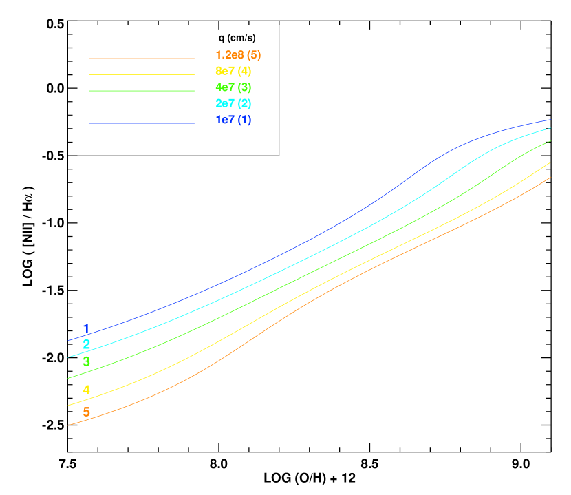
Figure 4: The metallicity-sensitive line ratio [N II]/H$\alpha$ versus the metallicity $12+\log(O/H)$. The colored curves show our new parameterization (equation 12) to the theoretical photoionization models of Kewley & Dopita (2003) for various values of ionization parameter, $q$, in cm s^-1 shown in the legend. Note that the [N II]/H$\alpha$ ratio is very sensitive to ionization parameter and is a not a robust indicator of metallicity. The metallicity corresponding to any particular value of [N II]/H$\alpha$ spans 0.4—0.6 dex in O/H, depending on ionization parameter.

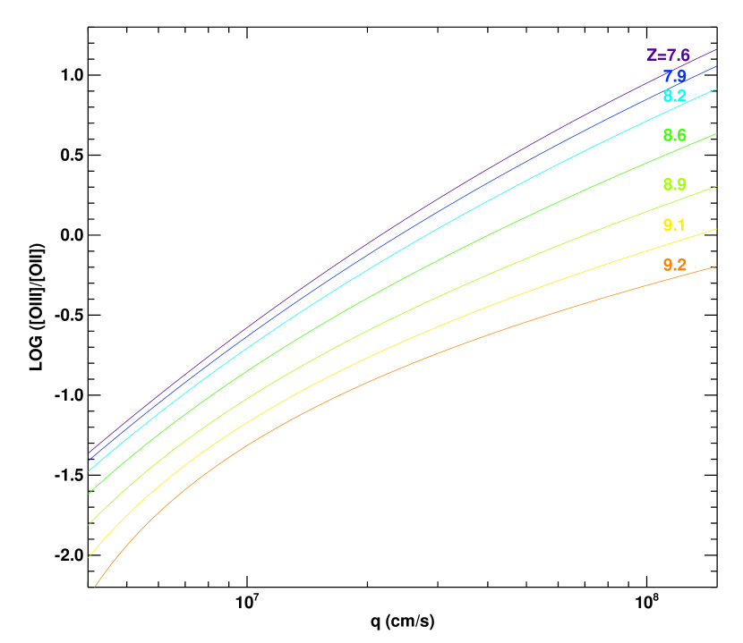
Figure 5: The [O III]/[O II] ratio versus ionization parameter, $q$, in cm s^-1. The colored curves show our new parameterization (equation 13) to the theoretical photoionization models of Kewley & Dopita (2003) for various values of metal mass fraction, $Z$, shown. The relation between $Z$ and O/H is discussed in Section 2.4 and Equation 11.

where $y=\log(O_{32})$. Figures 4 and 5 show the parameterizations in equations 12 and 13 for various values of ionization parameter. Equation 12 is only valid for ionization parameters $q$ between $5\times 10^{6}-1.5\times 10^{8}$ cm/s. KD03 show that for log([N II]/H$\alpha$)$>-0.8$, the [N II]/H$\alpha$$--$metallicity relationship breaks down. Although such high [N II]/H$\alpha$ ratios indicate that the metallicity is on the upper branch ($12+\log({\rm O/H})>8.4$), [N II]/H$\alpha$ cannot be used to estimate a metallicity in this regime. At lower [N II]/H$\alpha$ values, the [N II]/H$\alpha$ ratio is less sensitive to metallicity and is more dependent on the ionization parameter than the ${\rm R}_{23}$ ratio. Therefore, [N II]/H$\alpha$ should only be used as a crude initial estimate for a more sensitive metallicity diagnostic such as ${\rm R}_{23}$.

Because the [N II]/H$\alpha$ ratio depends strongly on the ionization parameter and the [O III]/[O II] ratio depends on metallicity, we iterated equations 12 and 13 until the metallicity varied less than the model errors ($\sim 0.1$ dex). Typically 2-3 iterations were required. The resulting metallicity estimates indicate that 29/32 (91%) of the galaxies with useable [N II]/H$\alpha$ ratios or upper limits lie on the upper ${\rm R}_{23}$ branch ($12+log(O/H)>8.4$). In column 20 of Table 5 we list the oxygen abundance derived from the strength of the [N II] $\lambda$6584/H$\alpha$ equivalent width ratios for the 35 (necessarily the lowest redshift) galaxies where these lines can be measured. In many cases, only 3$\sigma$ upper limits on the [N II] $\lambda$6584 equivalent widths are measured, so only upper limits on the oxygen abundances are given. Of the galaxies where [N II] can be measured, only 2 of the least luminous galaxies ($M_{B}\sim-17$) have [N II] $\lambda$6584/H$\alpha$ ratios consistent with very low metallicities that would place them on the lower branch of the $R_{23}$–O/H calibration. These objects are noted in Table 5.

For the TKRS galaxies without [N II]/H$\alpha$ ratios, we are unable to break the ${\rm R}_{23}$ degeneracy. We make the motivated assumption (see Kobulnicky & Zaritsky 1999, Kobulnicky et al. 2003) that these galaxies fall on the upper-branch ($12+log(O/H)>8.4$) of the double-valued $R_{23}-O/H$ relation, consistent with the majority of galaxies in our sample with [N II]/H$\alpha$ ratios. We next compute the oxygen abundances of TKRS galaxies using several different, independent but related ${\rm R}_{23}$–O/H calibrations from the literature.

2.4.1 Zaritsky, Kennicutt, & Huchra 1994, (ZKH)

Zaritsky, Kennicutt, & Huchra 1994, (ZKH) provide a simple analytic relation between O/H and $R_{23}$ only without regard to ionization parameter:

$$12+\log({\rm O/H})_{\rm ZKH}=9.265-0.33\,{R}_{23}-0.202\,{R}_{23}^{2}-0.207\,{R}_{23}^{3}-0.333\,{R}_{23}^{4}$$ (14)

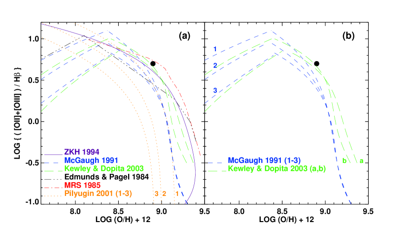
Figure 6: Metallicity calibration between strong line ratio $R_{23}$ and oxygen abundance, $12+\log(O/H)$ from several different authors as indicated in the legend. A solid circle marks the Orion Nebula value (based on data of Walter, Dufour, & Hester 1992). For reference, the currently accepted value of solar abundance is $12+\log(O/H)_{\odot}=8.7$ (Allende Prieto, Lambert, & Asplund 2001). Panel (a) shows the variation in ${\rm R}_{23}$ calibrations from the literature, while panel (b) shows the M91 and KD03 calibrations. The three curves labeled 1,2,3 denote the Pilyugin 2001 and M91 models corresponding to $\log({\rm O_{32}})=1,0,-1$ respectively. Two curves labeled a,b denote the Kewley & Dopita (2003) models corresponding to ionization parameters of $q=1\times 10^{7}$ and $q=1.5\times 10^{8}$ cm/s respectively.

The ZKH formula is an average of three previous calibrations in the literature, namely Dopita & Evans (1986), McCall, Rybski & Shields (1985), and Edmunds & Pagel (1984). Figure 6 shows these relations. The ZKH average relation was compared with a sample of disk H II regions with metallicities $\log({\rm O/H})+12$$>8.35$. As a result, the ZKH calibration is only suitable for H II regions in the metal-rich regime.

2.4.2 McGaugh 1991 (M91)

McGaugh (1991) calibrated the relationship between the $R_{23}$ ratio and gas-phase oxygen abundance using H II region models from the photoionization code CLOUDY (Ferland & Truran 1981). McGaugh’s models include the effects of dust and variations in ionization parameter. Adopting the analytical expressions of McGaugh (1991, 1998 as expressed in KKP) which are based on fits to photoionization models for the metal-rich (upper) branch of the $R_{23}$–O/H relation. In terms of the reddening corrected line intensities, this relation is

$$12+log(O/H)_{\rm M91,upper} = 12-2.939-0.2x-0.237x^{2}-0.305x^{3}-0.0283x^{4}-$$ (15)

$$y(0.0047-0.0221x-0.102x^{2}-0.0817x^{3}-0.00717x^{4}).$$

Figure 6 shows graphically the relation between $R_{23}$ and O/H for the McGaugh (1991) and other calibrations from the literature. A circle marks the Orion Nebula value (based on data of Walter, Dufour, & Hester 1992) which is in excellent agreement with the most recent solar oxygen abundance measurement of $12+log(O/H)_{\odot}=8.7$ (Prieto, Lambert, & Asplund 2001). Oxygen abundances computed in this manner appear in Table 5 column 17, along with a $1\sigma$ uncertainty computed by propagating the uncertainties on the emission line equivalent widths. This uncertainty estimate does not include the error introduced by the model uncertainties in the theoretical calibrations (typically $\sim 0.1$ dex).

2.4.3 Pilyugin (2001)

Pilyugin (2001) developed an $R_{23}$–O/H calibration based on a sample of H II regions with measurements of the [O III] $\lambda 4363$ auroral line. The [O III] $\lambda 4363$ auroral line provides a “direct” measurement of the electron temperature of the gas, and therefore, the metallicity. The use of the [O III] $\lambda 4363$ auroral line to derive metallicities is known as the T_e method. Pilyugin (2001) calculated direct metallicities for a sample of H II regions spanning $8.2\lesssim 12+\log(O/H)\lesssim 8.6$. His resulting $R_{23}$–O/H calibration provides three curves, depending on a parameter $P$ that accounts for the range in ionization parameter in the H II regions. Pilyugin was unable to provide a fit to H II regions for $12+\log(O/H)\gtrsim 8.6$ because high metallicity galaxies have weak or undetectable [O III] $\lambda 4363$ (see Stasinska 2002 for a discussion). Therefore, Pilyugin extrapolated the $8.2\lesssim 12+\log(O/H)\lesssim 8.6$ curves to higher metallicities. The Pilyugin curves are discussed further in Kennicutt, Bresolin, & Garnett (2003).

2.4.4 Kewley & Dopita (2003)

Kewley & Dopita (2003) provide a suite of abundance calibrations depending on the availability of particular nebular emission-lines. Their calibrations are based on a combination of stellar population synthesis models (Pégase and STARBURST99) and detailed photoionization models using the MAPPINGS code (Sutherland et al. 1993). Like M91, the KD03 models include the effects of dust. KD03 include separate calibrations for ionization parameter. KD03 point out that the $R_{23}$ curve is dependent on ionization parameter, while the common ionization parameter diagnostic ($O_{32}$) depends on metallicity. They advocate the use of an iterative scheme to solve for both quantities if only [O III], [O II] and H$\beta$ are available. We provide a new parameterization of the KD03 ${\rm R}_{23}$ method (from Section 4.3 in in KD03) with a similar form to the M91 calibration to facilitate metallicity estimation and comparisons to estimates made using M91. For the potential ionization parameter and metallicity range of our sample (Figure 3), the lower branch ($12+\log(O/H)<8.4$) is parameterized by:

$$12+\log({\rm O/H})_{\rm KD03,lower}=9.40+4.65x-3.17x^{2}-\log(q)(0.272+0.547x-0.513x^{2})$$ (16)

where $x=\log(R_{23})$. The upper branch (12+log(O/H)$\geq 8.4$) is parameterized by:

$$12+\log({\rm O/H})_{\rm KD03,upper} = 9.72-0.777x-0.951x^{2}-0.072x^{3}-0.811x^{4}-$$ (17)

$$\log(q)(0.0737-0.0713x-0.141x^{2}+0.0373x^{3}-0.058x^{4}).$$

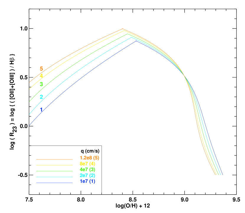
Figure 7: The metallicity-sensitive line ratio ${\rm R}_{23}$ versus the metallicity $12+\log(O/H)$. The colored curves show our new parameterization (equation 17) to the theoretical photoionization models of Kewley & Dopita (2003) for various values of ionization parameter, $q$, in cm s^-1 shown in the legend.

Figure 7 shows graphically the relation between the metallicity and ${\rm R}_{23}$ from equation 17 for various values of ionization parameter $q$ . The ionization parameter, $q$, is found using equation 13 in an iterative manner. Typically 2-3 iterations were required to reach convergence. This new parameterization is an improvement over the tabulated model coefficients of the KD03 calibration because (1) the new calibration does not fix the ionization parameter or metallicity to the finite set of model values during iteration, and (2) there is an increased sensitivity to the metallicity around the local maximum ($Z=8.4$) because we have introduced different equations for the two branches rather than being limited to one equation. Oxygen abundances calculated via this method are given in column 18 of Table 5. This parameterization should be regarded as an improved, implementation-friendly approach to be preferred over the tabulated $R_{23}$ coefficients of KD03.

2.4.5 “Best” Adopted Oxygen Abundances

Of all the above methods for oxygen abundance computation, many arguments could be made for which are the “best” or most “accurate”. In Figure 8 we compare the ‘P-method’, M91, ZKH and KD03 ${\rm R}_{23}$ metallicity estimates for the TKRS data. Differences between published calibrations shown in Figure 8 serve to illustrate the magnitude and severity of the possible systematic errors introduced by the different calibrations. The uncertainties from any published calibration method are dominated by systematic uncertainties and/or biases in the data and/or models used to construct the calibration. The ‘P-method’ produces a strong systematic offset and large scatter in the metallicity estimates compared to the three other calibrations. This offset probably occurs because the P-method was not calibrated using any data or theoretical models for the metallicity range of our sample. We therefore do not use the P-method in our preferred metallicity estimates.

The three remaining calibrations show smaller systematic offsets that are consistent with the error estimates of the calibrations ($\sim 0.1$ dex). Principle differences among the models include different photoionizing radiation fields from the various stellar atmospheres, stellar libraries, and stellar tracks. Different photoionization models employ various atomic data and dust prescriptions. Different calibration data from observations of Galactic or extragalactic H II regions over a range of metallicities and ionization parameters may also affect the resulting calibrations. Analyzing the nuances and resolving the differences between the published strong-line—metallicity calibrations is beyond the scope of this work. The exact choice of metallicity calibration is not crucial to the first of the two goals in this paper. Relative differences in metallicity between samples at different redshifts will not be sensitive to the exact form of the $R_{23}$–O/H calibration adopted. Section 3 below deals primarily with this question. Any of the three above methods which require only measurements of $R_{23}$ and $O_{32}$ will suffice for discerning trends with redshift.

Kennicutt, Bresolin, & Garnett (2003) and Garnett, Kennicutt, & Bresolin (2004) present evidence from observations of metal-rich H II regions in M 51 and M 101 that there is a discrepancy of several tenths of a dex (factor of 2 or more) between the metallicities derived using traditional strong line methods and models compared to methods using direct measurements of [N II] electron temperatures. See these works for an extensive discussion regarding possible systematic effects in the $R_{23}$–O/H calibrations. hence, absolute metal abundances may have systematic uncertainties of 0.2–0.5 dex, particularly at the high metallicity end of our sample. Until these initial results are confirmed and a more robust calibration is available, we proceed to adopt a combination of the KD03 and M91 strong line formulation.

For the purposes of providing the most meaningful metallicities to aid in modeling of distant galaxies, we adopt a final “best estimate” oxygen abundance by averaging the KD03 and M91 ${\rm R}_{23}$ methods; $12+\log({\rm O/H})_{\rm avg}=1/2[12+\log({\rm O/H})_{\rm KD03}+\log({\rm O/H})_{\rm M91}]$. We use the new KD03 parameterization (equations 17 and 13). Because the ZKH parameterization is based upon an ad-hoc average of 3 relatively old models and calibrations, we do not consider it for our best estimate in light of improvements to photoionization models (see for example Dopita et al. 2000, Kewley et al. 2001 and references therein).

The resulting average abundances appear in Table 5. For $12+\log({\rm O/H})>8.4$, the average of the KD03 and M91 methods can be approximated by the following simple form:

$$12+\log({\rm O/H})_{\rm avg-upper} \sim 9.11-0.218x-0.0587x^{2}-0.330x^{3}-0.199x^{4}$$ (18)

$$-y(0.00235-0.01105x-0.051x^{2}-0.04085x^{3}-0.003585x^{4})$$

where $x=\log(R_{23})$ (equation 8) and $y=\log(O_{32})$ (equation 10). Note that this equation is only valid for the upper branch, and for the range of ${\rm R}_{23}$ and ${\rm O}_{32}$ values covered by our sample (Figure 3).

2.5 Comparison with other properties

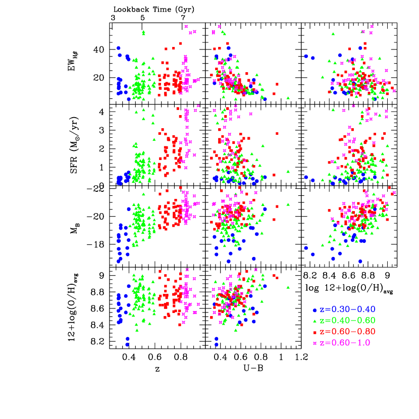
Figure 9: Distribution of $H\beta$ equivalent width, star formation rate, absolute B-band magnitude, oxygen abundance, U-B color, and redshift for the 204 selected TKRS galaxies.

Figure 9 shows the relations between the “best estimate” oxygen abundance, $H\beta$ equivalent width, star formation rate, absolute B-band magnitude, U-B color, and redshift for the 204 selected TKRS galaxies. This Figure illustrates that the colors and emission line equivalent widths of selected TKRS galaxies are distributed approximately uniformly across the full observed range of parameter space within each redshift bin. It also shows that galaxies at increasingly higher redshifts tend to be more luminous and have higher star formation rates. This is a type of selection effect due to the magnitude limited nature of the spectroscopic TKRS sample.

3 The L-Z Relation at $0.3<z<1.0$.

3.1 Evolution of the L-Z Relation

The addition of 204 new metallicities at $0.3<z<1.0$ allows us to explore more robustly than before the chemo-luminous evolution of galaxies over the last 8 Gyr. Figure 10 shows the oxygen abundance, $12+\log(O/H)_{M91}$ versus $M_{B}$ for four redshift ranges. Filled symbols show the DGSS data from Kobulnicky et al. (2003), crosses denote the CFRS data of LCS03 and CL01, and open symbols denote the TKRS data. Stars in the lower right panel are the $z>2$ Lyman break galaxies from Kobulnicky & Koo (2000) and Pettini et al. (2001). The dashed lines, which are the same in each panel, represent the fits to local emission line galaxy samples as described in Kobulnicky et al. (2003). The solid lines are fits to the DGSS data alone. The new TKRS data are in good agreement with the previous L-Z relations found for each redshift interval. It becomes possible, for the first time with these data, to see the L-Z correlation at redshifts $z>0.8$ in the lower right panel. The most significant departure from the DGSS L-Z correlation seen in the TKRS data occurs in the $0.4<z<0.6$ bin (lower left panel). There are galaxies located to the faint/metal-rich side of the best fit line in the TKRS sample which do not appear in the DGSS sample. This scatter is present to a lesser extent in the $0.6<z<0.8$ range (upper right panel). Examination of these objects in Table 5 reveals these to be mostly objects with extreme values of the ionization parameter indicator, $O_{32}$. Most of these galaxies have $\log O_{32}<-0.5$, placing them in an regime where the correlation between $R_{23}$ and $EWR_{23}$ (KP03, Figure 5) has a large dispersion and a systematic deviation from unity, making these points additionally uncertain. The conclusion of Figure 10 is to highlight the overall good correspondence of TKRS metallicities with other surveys for similar magnitude and redshift ranges.

Figure 11 shows our adopted oxygen abundances, $12+\log(O/H)_{avg}$, for the DGSS+CFRS+TKRS galaxies versus $M_{B}$ in each of four redshift intervals. Lines now represent fits to the combined data in each redshift interval. The dotted line is a fit of $M_{B}$ on O/H, the dashed line is the inverse fit of O/H on $M_{B}$. Since neither metallicity uncertainties nor the magnitude uncertainties are well characterized, we also use the method of linear bisectors described by Isobe et al. (1990), shown by the solid line. Parameters for the linear fits appear in Table 5. The fits show that, regardless of the fitting method adopted, there is evidence that the slope of the L-Z correlation changes with redshift. For the linear bisector fits, the L-Z relation evolves monotonically from $12+\log(O/H)=-0.164\pm 0.031\times M_{B}+5.57$ in the lowest redshift bin to $12+\log(O/H)=-0.241\pm 0.030\times M_{B}+3.73$ in the highest redshift bin. For the O/H on $M_{B}$ fits, the L-Z relation evolves monotonically from $12+\log(O/H)=-0.074\pm 0.032\times M_{B}+7.20$ in the lowest redshift bin to $12+\log(O/H)=-0.134\pm 0.032\times M_{B}+5.97$ in the highest redshift bin. This change is driven mainly by the appearance of a population of relatively luminous ($M_{B}\sim-20$) but metal-poor ($12+log(O/H)$=8.5–8.6) galaxies in the two highest redshift bins. Ke03 reported this change in slope of the L-Z relation using data out to $z=0.8$, and Figure 11 shows that this trend continues to higher redshifts. Based on plausible galaxy evolution models, optical morphologies, and their present metallicities, this population of galaxies is likely to evolve at roughly constant luminosity into comparatively metal-rich disk galaxies in the local universe rather than fade into “dwarf” galaxies (see Ke03, LCS03).

The evolution of mean galaxy metallicity with redshift can be seen more easily in Figure 12 which shows oxygen abundance, $12+\log(O/H)_{avg}$, versus redshift for three different luminosity bins. The upper row displays only distant galaxies, $z>0.3$. Lines show least squares fits to the data with errors in O/H only. The left panel shows the lowest luminosity galaxies with $-18.5>M_{B}>-19.5$. The slope of the least squares linear fit is -0.19$\pm 0.10$ dex per unit redshift. The linear correlation coefficient for the 60 galaxies in this panel is -0.201, indicating that the probability of obtaining such a strong correlation at random is 12%. For the middle panel showing 100 galaxies in the luminosity range $-19.5>M_{B}>-20.5$, the best fit slope is -0.19$\pm 0.08$ dex per unit redshift. The correlation coefficient is -0.228, indicating that the probability of exceeding this degree of correlation by chance is 2%. For the right panel showing 69 galaxies in the luminosity range $-20.5>M_{B}>-21.5$, the best fit slope is -0.18$\pm 0.09$ dex per unit redshift. The correlation coefficient is -0.197, indicating that the probability of exceeding this degree of correlation by chance is 10%. Note that the relation between redshift and mean galaxy metallicity may not be (indeed, is theoretically not expected to be) a linear one if the star formation rate is not a linear function of redshift (e.g., Somerville 2001). However, the observed dispersion and limited range of luminosity and redshift of the current data do not warrant additional parameters in the fit.

The lower row of Figure 12 shows the same galaxies as the upper row, but with the addition of local $z=0$ galaxies from Kennicutt (1992) and Jansen et al. (2001) used by Ke03 to define the local L-Z relation. Lines show least squares fits to the sample. The slopes are now somewhat smaller, 0.14$\pm 0.05$ dex/z for the low- and intermediate-luminosity bins and 0.13$\pm 0.05$ dex/z in the high-luminosity bin. This high-luminosity bin lacks the population of low-redshift ($0.3<z<0.6$), low-metallicity (12+log(O/H)¡8.7) galaxies present in the middle and left panels. It is this population, or rather the lack thereof, which is responsible for the change in slope of the L-Z relation in Figures 10 and 11. The metallicities of the most luminous objects could be described as reaching a plateau near $12+log(O/H)=8.9$ with increasing scatter to lower oxygen abundances at larger redshifts. Such a plateau is expected in chemical evolution models as galaxies expend their gas supplies near the cessation of star formation activity. However, this plateau may also be a consequence of the $R_{23}$ to O/H formulation (Figure 6) which asymptotes at high metallicities, folded with observational selection effects which will preferentially exclude very high metallicity objects which have very weak [O III] emission lines.

The mean rate of metal enrichment observed in Figure 12 is at least 0.14 dex per unit redshift for all luminosity bins. This rate of metal enrichment is significantly greater (2-3$\sigma$) than the increase of $0.08\pm 0.02$ dex estimated by Lilly, Carollo, & Stockton (2003) over the same redshift interval. The smaller ${d(O/H)}\over{dz}$ measured by LCS03 stems from the fact that 1) the mean luminosity of the LCS03 sample would lie in our high-redshift bin ($-20.5<M_{B}<-21.5$), and 2) LCS03 compare the oxygen abundance average (weighted by the H$\beta$ luminosity) of relatively luminous $M_{B}<-19.5$ CFRS galaxies with an average of NFGS galaxies spanning a range of luminosities from $M_{B}=-16$ to $M_{B}=-22$. The inclusion of these low luminosity galaxies in the local mean reduces the metallicity difference between the local and distant samples.

3.2 The Effects of Sample Selection

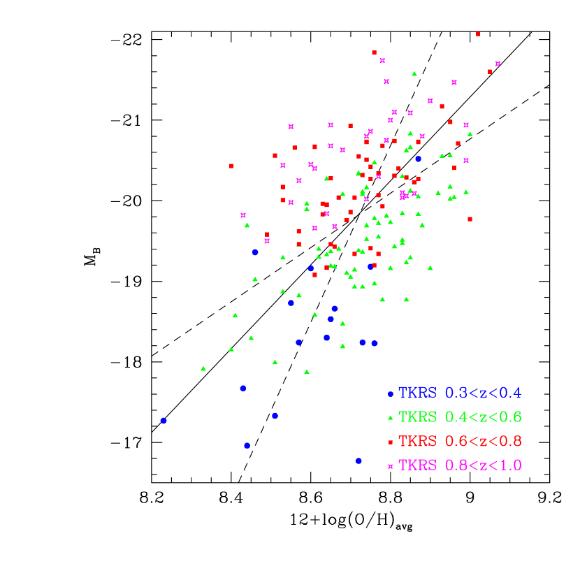
Figure 14: L-Z relation for 177 TKRS galaxies with symbols denoting the four redshift bins. Dashed lines are unweighted linear least squares fits of x-on-y and y-on-x, while the solid line is the linear bisector of the two fits. This figure shows that the highest redshift TKRS galaxies lie systematically to the bright/metal-rich side of the overall L-Z relation.

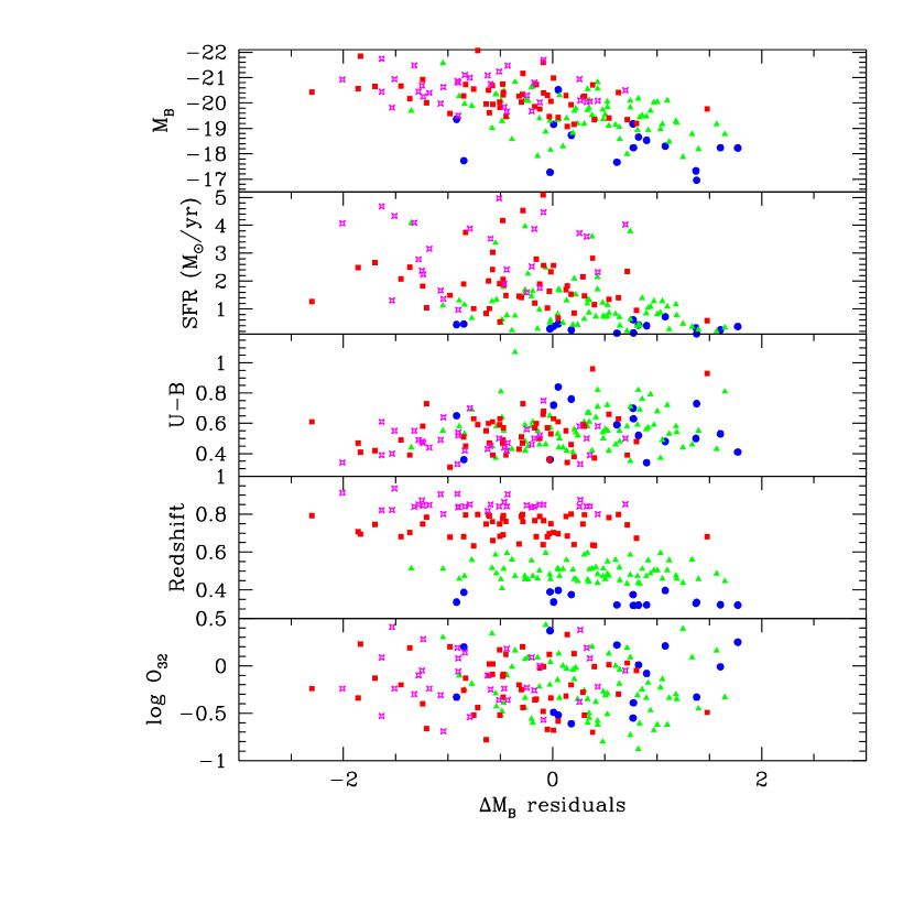
Figure 15: Magnitude residuals, $\Delta M_{B}$, from the best-fit luminosity-metallicity relation in Figure 14 for 177 TKRS galaxies as a function of luminosity, star formation rate, color, redshift, and ionization parameter indicator, $O_{32}$. Symbols denote redshift bins. There is a strong correlation between magnitude residuals and the three closely related parameters $z$, $SFR$, and $M_{B}$. There is no correlation between residuals and U-B or $O_{32}$.

Could some selection effect in the chosen galaxy sample produce the signature of evolution in the L-Z relation? Kobulnicky et al. (2003) discuss possible selection effects in the Deep Groth Strip Survey sample and conclude that no identifiable selection effect can produce the observed signature of chemo-luminous evolution with cosmic epoch. Here we test the TKRS sample for selection effects which could mimic the signature of genuine evolution in the L-Z relation. Figure 14 shows the correlation between luminosity and $12+\log(O/H)$ for 177 TKRS galaxies coded by redshift interval. Dashed lines are unweighted linear least squares fits of x-on-y and y-on-x, while the solid line is the linear bisector of the two fits. This figure shows that the highest redshift TKRS galaxies lie systematically to the bright/metal-rich side of the overall L-Z relation. To examine whether some parameter other than redshift might be responsible for this trend, we show in Figure 15 the magnitude residuals from the best fit L-Z relation (solid line in Figure 14) as a function of other fundamental galaxy parameters: $M_{B}$, star formation rate, U-B color, redshift, and ionization parameter indicator $O_{32}$. There is no correlation between magnitude residuals and $U-B$ or $O_{32}$. There is a strong correlation between magnitude residuals and $z$, SFR, and $M_{B}$. These three parameters are not independent quantities. As noted in the discussion of Figure 9, $M_{B}$ is tightly coupled with $SFR$ because it is used, along with $EW_{H\beta}$, to calculate the star formation rate. The $SFR$ scales with $M_{B}$. Redshift and the mean $M_{B}$ at a given redshift are also closely coupled by the characteristics of a magnitude-limited survey. Figures 2 and 9 illustrate that galaxies as faint as $M_{B}=-17$ populate the lowest redshift bin while the highest redshift bin contains no objects fainter than $M_{B}=-19.5$. The lowest redshift bin also lacks the population of luminous $M_{B}=-22$ galaxies found at larger distances. The correlations in Figure 15, then, may all be understood as a consequence of a single underlying cause, namely the inter-relation between $z$, $M_{B}$, and $SFR$ among sample galaxies.

Which of the three parameters is the fundamental one driving the observed change in the L-Z relation? We argue that redshift is fundamental. Because the least squares fit in Figure 14 uses $M_{B}$ as one of the correlative variables, residuals should not depend on $M_{B}$. If the star formation rate were the fundamental parameter driving the evolution of the L-Z relation (i.e., galaxies with the highest star formation rates preferentially lie on the bright/metal-poor side of the L-Z relation), then we would also expect related parameters like the U-B color, which is sensitive to the star formation rate, to show a correlation with $\Delta M_{B}$ as well. Figure 15 shows that $U-B$ is not correlated with $\Delta M_{B}$. We are left with the conclusion that the evolution of the L-Z relation is driven primarily by the redshift of the galaxies under consideration. Galaxies of a given luminosity are, on average, increasingly metal poor at higher redshifts. Said another way, galaxies of a given metallicity are, on average, more luminous at higher redshifts. This effect is most pronounced among the least luminous galaxies, those with $M_{B}$ fainter than $\sim-20$. None of the identified sample selection effects would produce the changes in the nature of the L-Z relation seen in Figures 11 and 12.

3.3 Comparison to Metallicity Evolution in the Milky Way

One goal of studying galaxy populations at cosmological distances is to understand the evolutionary paths of individual galaxies. However, observing the evolution of the mean chemo-luminous properties of the population of star-forming galaxies over the last 8 Gyr (Figure 11, 12) is not the same thing as observing the evolution of any particular galaxy. Events shaping the evolution of any given galaxy at any particular point in its history, could, in principle, be unique to that galaxy and not be reflected in the mean properties of galaxies at the equivalent lookback time in the distant universe. A galaxy, may, for example, spend most of its existence in a quiescent passively evolving phase after a brief initial period of star formation. Other galaxies might form stars continuously throughout their existence, while still others may not begin the star formation process until comparatively recent times. However, if the boundary conditions for galaxy evolution are determined primarily by global cosmological parameters, such as the age of the universe, the expansion rate, and the density of dark matter and gas available to form stars, then evolutionary paths of most galaxies ought to be observable in the mean evolution of galaxy properties with redshift.

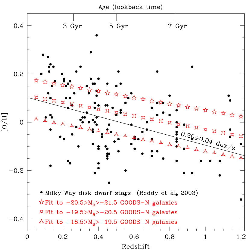
Figure 13: Relation between age (a.k.a lookback time) and oxygen abundance, relative to solar, for Milky Way disk stars from Reddy et al. (2003). The ages of the stars are plotted in terms of their equivalent redshifts (using the adopted cosmology) for direct comparison to Figure 12. The line shows a least squares linear fit to the Galactic data. The tracks of symbols show the fits from Figure 12 (lower row) for galaxies in three different luminosity bins. The mean slope and zero point for the evolution of Milky Way stars are in good agreement with the overall metallicity and rate of enrichment for distant galaxies.

Measuring ages and chemical abundances of stars in the Milky Way provides a glimpse into the history of one, presumably typical, disk galaxy. Figure 13 shows [O/H], the logarithmic oxygen abundances relative to solar, of F and G stars in the Galactic disk as a function of age (Reddy et al. 2003). We have plotted on the ordinate the redshift corresponding to the lookback time of the measured age of the star. For our adopted cosmology of $H_{0}=70$ km s^-1 Mpc^-1, $\Omega_{M}=0.3$, $\Omega_{\Lambda}=0.7$, the relation between redshift, $z$, and the lookback time or age, $a$, in Gyr is closely approximated by a polynomial,

$$z=1.3356-2.0847a+1.2431a^{2}-0.33620a^{3}+0.046737a^{4}-0.0032106a^{5}+0.000086938a^{6}.$$ (19)

The solid line shows the least squares O/H on $z$ fit to the stellar measurements. The tracks of starred symbols show the least-squares linear fits to distant GOODS-N+CFRS+TKRS galaxies in the three luminosity bins from the lower row of Figure 12. We use [O/H] = 12+log(O/H) -8.7 in keeping with the most recent solar oxygen abundance measurements (Allende-Prieto et al. 2001). Both the overall level of metal enrichment (zero point) for $M_{B}\sim 20$ galaxies and the rate at which oxygen abundance increases with time (slope) among all GOODS-N galaxies over the redshift range $z$=1–0 agree well with the trend observed in Galactic stars. The slopes of the best fit relations for galaxies from the lower panel of Figure 12, $0.14\pm 0.05$ dex, are within the uncertainties of the slope for Milky Way stars, $0.20\pm 0.04$ dex over the range $0.0<z<1.0$.

LCS03 presented a diagram similar to Figure 13 where they compare CFRS and NFGS oxygen abundances to [Fe/H] measurements of Galactic disk stars and noted that the stars were consistently 0.2-0.3 dex more metal poor than the galaxies. This offset may be understood as the signature of super-solar O/Fe ratios found in Galactic stars over most of the history of the Milky Way reflecting varying nucleosynthetic sources (reviewed by Wheeler, Sneden, & Truran 1989). Using oxygen measurements for Milky Way stars in Figure 13 shows good agreement with the oxygen abundance measurements in distant galaxies. While the luminosity history of the Milky Way is not known, and while the dispersion in oxygen abundances for Galactic stars is large, the chemical enrichment process that occurred in the disk of the Milky Way appears to be a good representation of the chemical enrichment process in the bulk of the star-forming galaxies over the last 8 Gyr. Ke03 observed that the majority of the star–forming galaxies in the DEEP Groth Strip Survey over a similar redshift range appeared to have substantial disk components based on Hubble Space Telescope imaging. Thus, it appears we are able to observe directly, in ensembles of disk-like galaxies at cosmological distances, the same chemical histories encoded in Galactic stellar populations. In general, we expect that the luminosity-weighted nebular oxygen abundance of the entire Milky Way would be 0.1–0.3 dex higher than the metallicity of the solar neighborhood, given that the bulk of star formation occurs in the molecular ring at smaller radii where the average composition is more metal rich (e.g., Shaver et al. 1983; Maciel, DaCosta, & Uchida 2003).

For a galaxy that evolves as a “closed box” (i.e., no gas inflow or outflow), converting gas to stars with a fixed initial mass function and chemical yield, the metallicity is determined by a single parameter: the gas mass fraction, $\mu=M_{gas}/(M_{gas}+M_{stars})$. The metallicity, $Z$, is the ratio of mass in elements heavier than He to the total mass and is given by

$$Z=Y~{}ln(1/\mu),$$ (20)

where $Y$ is the “yield” as a mass fraction. A typical total metal yield for a Salpeter IMF integrated over 0.2–100 $M_{\odot}$ is $Y=0.012$ by mass (i.e., 2/3 the solar metallicity of 0.018; see Pagel 1997, Chapter 8). A total oxygen yield for the same IMF would be $Y_{O}=0.006$. Effective yields in many local galaxies range from solar to factors of several lower (Kennicutt & Skillman 2001; Garnett 2002). The change in metallicity with gas mass fraction is independent of yield and is given by

$${{d\log Z}\over{d\mu}}={{d}\over{d\mu}}~{}\big{[}Y~{}ln({{1}\over{\mu}})\big{]}={{0.434}\over{\mu~{}ln(\mu)}}.$$ (21)

For reasonable values of the gas mass fraction (0.1-0.3), the change in gas mass fraction, $\Delta\mu$, corresponding to $\Delta\log(Z)=0.14$ is 0.07 to 0.12. Such a change in average gas content should be observable with future radio wave interferometers.

3.4 Comparison to Expectations of Cosmic Star Formation Models

The observed 0.14 dex increase in oxygen abundance of galaxies from $z=1$ to $z=0$ is equivalent to a 38% increase in metallicity since $z=1$. In other words, 28% of the metals in $z=0$ star-forming galaxies $-18.5<M_{B}<20.5$ have been produced in the last 7.7 Gyr since $z=1$. This conclusion can be tested for consistency against expectations from the global rate of cosmic star formation over the same period. Given that the magnitude range of our sample encompasses the bulk of luminosity produced by all galaxies (given a typical local galaxy luminosity function), the observed 28% increase in metal content should reflect the overall level of chemical enrichment in the universe. The rate of metal enrichment should correlate directly with the rate of star formation, subject to the condition that the stellar initial mass function and the chemical yield per mass of stars formed is constant.

The cosmic rate of star formation as a function of redshift has been extensively studied, and we adopt, for illustrative purposes, the models from Figure 9 of Somerville et al. (2001). Figure 16 shows the star formation rate versus time for their “collisional starburst” and “accelerated quiescent” models which give reasonable agreement with the observations. We have transformed redshift into linear time on the ordinate, using our adopted cosmology, and plotted linear star formation rate on the abscissa. The shaded regions in each figure show the integral of the star formation rate over time from $z=0$ to $z=1$ (0 Gyr to 7.7 Gyr lookback time). The fraction of all stars formed in the last 7.7 Gyr, $f_{*}({{z1-0}\over{z6-0}})$, is 0.38 and 0.42 in the two models. This fraction compares favorably with the fraction of metals formed during the same time period, $0.28\pm 0.07$, from the previous section. Any difference, if real, between the predicted fraction based on star formation rate indicators and the observed fraction may be explained in several ways.

• The present data/models may be underestimating the fraction of star formation which occurred before $z=1$. A star formation rate which is, on average, not more than 10% higher at $z>1$ would be required to produce agreement.

• The stellar initial mass function or metal yield may vary with redshift so that the assumption of a linear relationship between star and metal production is violated. A stellar initial mass function which is more shallow or more top heavy, or a higher effective nucleosynthetic yield at $z>1$ would be required.

Given the significant uncertainties on the star formation rate and the metal enrichment rate in galaxies as a function of redshift, no firm conclusion can be drawn except to say that the two rates are generally consistent with one another. Given that all models and data on the star formation rate (e.g., see Figure 16 and the summary in Somerville et al. 2001) show a decline in the star formation rate with time after $z=1$, the rate of metal enrichment in galaxies should also drop. In principle, this drop in the rate of metal enrichment should be observable in chemical studies of galaxies at cosmological distances, but will require a level of measurement precision and/or a sample size beyond current capabilities.

4 Discussion

Our findings with the GOODS-N data here are in agreement with the conclusions of Ke03, namely that chemo-luminous evolution is most pronounced among the least luminous (and possibly the least massive) galaxies during the 8 Gyr since $z\sim 1$. The change in slope of the L-Z relation with redshift in Figure 11 is due to the emergence of a population of moderately luminous ($M_{B}\sim-20$) galaxies with intermediate metallicities (12+log(O/H)$\sim 8.5-8.6$) at redshifts beyond $z=0.6$ which are not seen in local samples. This observation is consistent with the conclusions of LCS03 who advocate a progression of star formation activity from massive galaxies to less massive galaxies with decreasing redshift, a process generically termed as “downsizing” (Cowie et al. 1996). In the context of single-zone Pégase2 galaxy evolution models, Kobulnicky et al. (2003), concluded that the change in slope of the L-Z relation could be explained by at least two of the following three phenomena: 1) low-mass galaxies have lower effective chemical yields than massive galaxies, 2) low-mass galaxies assemble on longer timescales than massive galaxies, 3) low-mass galaxies began the assembly process at a later epoch than massive galaxies, i.e., “downsizing”. The possibility that low mass galaxies begin their assembly at a later cosmic epoch has received several independent sources of support, both theoretical and observational. Babul & Rees (1992) proposed a theoretical model whereby photoionization from the first generations of cosmic star formation keeps gas in galaxies with small potential wells ionized (and thus unable to form stars) until some relatively late epoch, approximately $z=1$. Skillman et al. (2003) concluded from an Hubble Space Telescope study of the star formation history in the Local Group galaxy IC 1613 that its star formation may have been inhibited until $z\sim 1$. Kodama et al. (2004) concluded from color-magnitude relations that galaxies in the Subaru/XMM Deep Survey were consistent with “downsizing” scenario as well.

Can the evidence for the “downsizing” scenario be predicted or modeled theoretically? Theoretical hydrodynamic simulations have been used recently to predict the variation of metallicity with redshift for Damped Lyman $\alpha$ (DLA) absorbers (e.g., Nagamine, Springel, & Hernquist 2004) or for the stellar metallicity of galaxies (e.g., Nagamine, Fukugita, & Ostriker 2001). Unfortunately, the current models suffer from a lack of resolution in the $0<z<1$ range. The direct simulations by Nagamine et al. predict that the mean metallicity at $z=1$ is $\sim 0.4$ ${\rm Z}_{\odot}$, corresponding to $\log({\rm O/H})+12$$\sim 8.3$, significantly lower than the metallicities of our sample, even at $z$ close to 1. However, both absorption line measurements and simulations of chemical abundances in DLA systems are not directly comparable to emission line measurements because the former probe the more extended gaseous halos surrounding galaxies while the latter probe the H II regions and sites of active star formation within the inner disks of galaxies. These chemical measurements of galaxies in the GOODS-N provide a significant dataset for comparison with future cosmological simulations which will have the temporal and spatial resolution to track the composition of the galaxies on 10 kpc scales with redshift.

5 Conclusions

We have parameterized an updated analytic formulation of the $R_{23}$–O/H relations for estimating nebular oxygen abundances based on the photionization models of Kewley & Dopita (2003). After reviewing existing calibrations, we also provide a parameterization for the average of this calibration and that of McGaugh (1991) for the upper branch only. An additional parameterization may be used to estimate, albeit very crudely, the metallicities of galaxies based on the nebular [N II]/H$\alpha$ ratios.

Analyzing spectra of 204 galaxies at $0.3<z<1.0$ from the GOODS-N TKRS, we measure galaxy-averaged nebular oxygen abundances of $8.2<12+\log(O/H)<9.1$, corresponding to metallicities between 0.3 and 2.5 times the solar value. The overall oxygen abundance of galaxies in the luminosity range $-18.5<M_{B}<-21.5$ increases by 0.14$\pm$0.05 dex from $z=1$ to $z=0$. Said another way, galaxies in this intermediate-redshift sample are 1-3 magnitudes more luminous at a given metallicity than are local counterparts. For closed box chemical evolution models, the implied change in gas mass fraction, $\mu$, over the $z=$1–0 interval as gas is cycled through stars to produce heavy elements is $\Delta\mu\sim 0.10$. This sample of galaxies exhibits a luminosity-metallicity correlation, but with different zero points, and possibly different slopes at each redshift interval. The change in slope is driven mostly by the appearance of a population of moderate luminosity ($M_{B}\sim-20$) galaxies at $z>0.6$ with intermediate metallicities (12+log(O/H)=8.5-8.6). This population is likely to evolve into the comparatively luminous, metal rich disk galaxy population of today. This change in galaxy populations is consistent with a later formation epoch for lower mass galaxies. The increase in the mean oxygen abundance of $-18.5<M_{B}<-21.5$ galaxies is broadly consistent with the global picture of cosmic star formation activity which suggests that $\sim 38$% of the stars and $\sim 28\pm 0.07$% of the metals in the universe have formed in the 7.7 Gyr since $z=1$.

Figure 1: Histogram of 204 galaxies selected for chemical analysis (large symbols) compared to the total 1044 objects in the TKRS survey survey with spectroscopic redshifts $0.3<z<1.0$. We show the distribution as a function of redshift, observed i-band magnitude, $M_{B}$, and U-B color. This figure demonstrates that galaxies selected as suitable for chemical analysis are reasonably representative of the larger TKRS sample in GOODS-North field in terms of their redshift distributions, magnitudes, and luminosities. However, the 204 selected galaxies preferentially have bluer U-B colors consistent with higher rates of star formation, and they comprise a disproportionate fraction of galaxies near the faint end of the survey limit at $R\sim 24$.

Figure 2: Distribution of apparent magnitude, U-B color, and B-band luminosity as a function of redshift for 204 galaxies selected for chemical analysis (large symbols) and the 1044 objects in the TKRS survey with spectroscopic redshifts $0.3<z<1.0$ (dots).

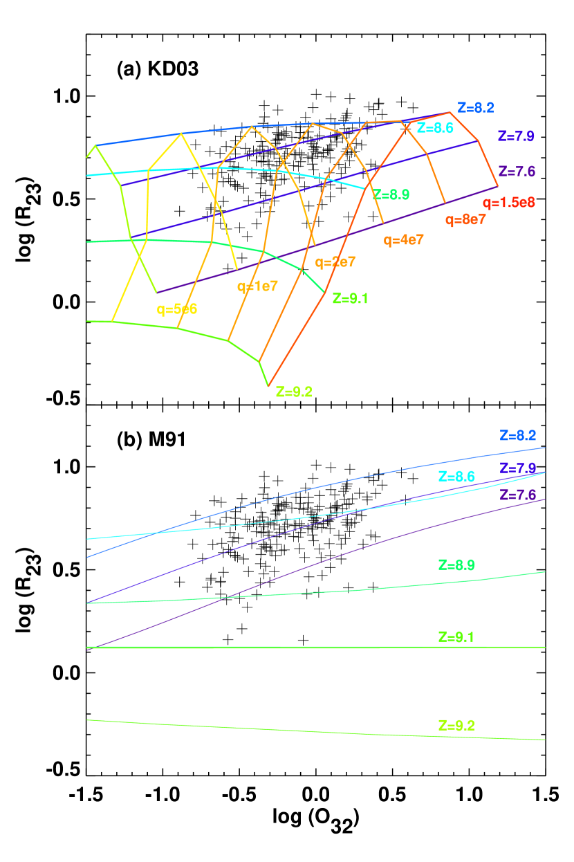
Figure 3: The logarithm of the metallicity-sensitive line ratio $R_{23}$ versus the logarithm of the ionization-parameter sensitive ratio $O_{32}$ for the TKRS galaxies. The colored curves represent the theoretical photoionization models of (a) Kewley & Dopita (2003) and (b) McGaugh (1991). Models are shown for metallicities between $12+\log(\rm{O/H})=7.6$ (violet) to $12+\log(O/H)=9.1$ (green). For reference, solar metallicity is $12+\log(\rm{O/H})\sim 8.7$ (Allende Prieto et al. 2001). The Kewley & Dopita (2003) models for ionization parameters between $q=5\times 10^{6}-1.5\times 10^{8}$ cm/s are shown (yellow-red curves). The TKRS data span ionization parameters $q=1\times 10^{7}-8\times 10^{7}$ cm/s.

Figure 8: Comparison of difference oxygen abundance computation methods for TKRS galaxies. The solid y=x line indicates where the data would lie if the different metallicity estimates reach agreement. The ‘P-method’ proposed by Pilyugin (2001) produces a strong systematic offset and significant scatter compared to the other three calibrations: McGaugh (1991; M91), Zaritsky, Kennicutt & Huchra (1994; ZKH94), and Kewley & Dopita (2003; KD03). Overall, the M91, ZKH94 and KD03 methods (with our new parameterization of the KD03 ${\rm R}_{23}$ and [O III]/[O II]models) produce metallicity estimates that reach agreement to within the error estimates for the calibrations ($\sim 0.1$ dex each). The ZKH94 method should not be used for $12+\log(O/H)<8.35$ because the ZKH94 method places these galaxies on the upper ${\rm R}_{23}$ branch.

Figure 10: Relation between blue luminosity and oxygen abundance in four redshift bins for the TKRS galaxies in the GOODS-North field (open symbols), the DEEP Groth Strip Survey from Kobulnicky et al. (DGSS, 2003; filled symbols), and the Canada-France Redshift Survey from Lilly et al. (2003; crosses) and Corollo & Lilly (2002; crosses). Broken symbols denote 3$\sigma$ O/H lower limits for TKRS galaxies with [O III]$\lambda$5007 non-detections. Solid lines are fits to the DGSS data from Ke03 and dashed lines are fits to the local galaxies samples defined in Ke03. This figure shows oxygen abundances from column 17 of Table 5. Stars denote the high redshift $z>2$ galaxies from Kobulnicky & Koo (2000) and Pettini et al. (2001). The TKRS data are consistent with the previous results from smaller datasets.

Figure 11: Relation between blue luminosity and oxygen abundance as in Figure 10 except that oxygen abundances are $(O/H)_{avg}$ from column 19 of Table 5. Dotted and dashed lines are linear least squares fits for x-on-y and y-on-x while the solid lines are linear bisectors of the two fits. Parameters of the fits appear in Table 5.

Figure 12: Relation between redshift and oxygen abundance for TKRS plus CFRS (LCS03) and DGSS (Ke03) galaxies in three different luminosity ranges. The upper row shows only distant galaxies. Large open symbols indicate mean values in two redshift bins: $z<0.6$ and $z>0.6$. The lower row shows the same data with a sample of local $z=0$ galaxies from Jansen et al. (2001) and Kennicutt (1992) as defined by Ke03. The slopes of least squares fits are given in each panel. The evolution of mean oxygen abundance with redshift is $\sim 0.19$ dex/z in the upper row and is consistent across redshift bins. When local galaxies are considered, the slopes of the metallicity-redshift relations in all bins drop to $\sim 0.14\pm 0.05$ dex/z.

Figure 16: Star formation rate density as a function of time, for our adopted cosmolgy, based on two models from Figure 9 of Somerville et al. (2001). The shaded regions in each figure show the integral of the star formation rate over the period from $z=0$ to $z=1$ (0 Gyr to 7.7 Gyr lookback time). The fraction of all stars formed in the last 7.7 Gyr, $f_{*}({{z1-0}\over{z6-0}})$, is 0.38 and 0.42 respectively, for the “collisional starburst” and “accelerated quiescent” models.

Table 1: GOOD-North TKRS Selected Galaxies

	ID	GOODS ID	z	${R}$	$i_{775W}$	$M_{B}$	$U-B$	$EW$	$EW$	$EW$	$EW$	$SFR$	code	$log(O_{32})$	$R_{23}$	$O/H$	$O/H$	$O/H$	$O/H$	$O/H$
				mag	mag	mag	mag	$[O~{}II]$	$H\beta$	$[O~{}III]$	Hα/NII	$M_{\odot}/yr$				$M91$	$KD$	$avg$	$N\sc{II}$	$final$
(1)	(2)	(3)	(4)	(5)	(6)	(7)	(8)	(9)	(10)	(11)	(12)	(13)	(14)	(15)	(16)	(17)	(18)	(19)	(20)	(21)
1	3551	J123651.06+621732.0	0.31870	22.57	22.12	-18.24	0.630	40.9$\pm$2.1	6.6$\pm$ 0.5	16.5$\pm$ 0.7	7.1	0.14	0	-0.39	6.67	8.5$\pm$0.04	8.65	8.57	8.63	8.57$\pm$0.15
2	3792	J123656.21+621743.2	0.31911	24.21	24.00	-16.77	0.480	79.4$\pm$6.5	39$\pm$ 1.9	157.8$\pm$ 1.8	$\cdots$	0.22	0	0.29	5.78	8.66$\pm$0.02	8.79	8.72	$\cdots$	8.72$\pm$0.15
3	9483	J123652.47+621036.0	0.32036	22.18	21.89	-18.66	0.520	46.7$\pm$4.9	13.3$\pm$ 1.3	47.9$\pm$ 1.5	10.43	0.43	0	0.01	6.18	8.59$\pm$0.04	8.73	8.66	8.62	8.66$\pm$0.15
4	7972	J123658.06+621300.8	0.32040	22.73	22.45	-18.23	0.410	36.7$\pm$3.4	17.1$\pm$ 1.3	65.8$\pm$ 1.7	17.35	0.37	0	0.25	5.36	8.69$\pm$0.02	8.83	8.76	8.46	8.76$\pm$0.15
5	11168	J123704.28+621000.0	0.32129	23.35	23.07	-17.67	0.590	45.2$\pm$7.4	10.4$\pm$ 1.2	75.3$\pm$ 1.5	$>$7.16	0.13	0	0.22	9.71	8.36$\pm$0.07	8.51	8.43	$<$8.96	8.43$\pm$0.16
6	11004	J123703.91+621009.7	0.32144	22.45	22.21	-18.53	0.340	54.4$\pm$3.1	14$\pm$ 1.1	45.1$\pm$ 1.4	$>$9	0.4	0	-0.08	6.21	8.58$\pm$0.03	8.72	8.65	$<$8.65	8.65$\pm$0.15
7	12136	J123744.51+621411.1	0.32238	22.62	22.28	-18.24	0.530	37.7$\pm$3.8	11.5$\pm$ 1.0	36.3$\pm$ 1.3	10.46	0.25	0	-0.01	5.48	8.66$\pm$0.04	8.8	8.73	8.61	8.73$\pm$0.15
8	7105	J123715.86+621559.8	0.32930	23.58	23.38	-17.33	0.500	59.3$\pm$9.9	33.9$\pm$ 2.3	255.3$\pm$ 3.2	$>$7.08	0.32	0	0.63	8.76	8.5$\pm$0.03	8.52	8.51	$<$8.56	8.51$\pm$0.15
9	5152	J123725.33+621925.6	0.33519	24.22	23.66	-16.96	0.730	112.7$\pm$13.0	16.3$\pm$ 2.2	51.8$\pm$ 2.6	$\cdots$	0.11	0	-0.33	8.98	8.31$\pm$0.10	8.57	8.44	$\cdots$	8.44$\pm$0.18
10	9208	J123717.27+621356.8	0.33635	21.59	21.20	-19.36	0.650	49.8$\pm$3.9	7.2$\pm$ 0.9	23.0$\pm$ 0.9	8.35	0.44	0	-0.33	7.91	8.41$\pm$0.07	8.51	8.46	8.59	8.46$\pm$0.16
11	2476	J123617.96+621457.6	0.33690	21.48	21.06	-19.16	0.720	45.7$\pm$5.2	7.5$\pm$ 1.2	14.7$\pm$ 1.2	6.37	0.38	0	-0.49	6.35	8.52$\pm$0.09	8.68	8.60	8.64	8.6$\pm$0.17
12	1563	J123617.44+621551.6	0.37584	22.03	21.62	-19.18	0.700	51.9$\pm$1.4	11.8$\pm$ 0.5	14.3$\pm$ 1.4	3.86	0.61	2	-0.55	4.79	8.66$\pm$0.14	8.85	8.75	8.79	8.75$\pm$0.2
13	6493	J123704.02+621523.6	0.37593	22.53	22.08	-18.73	0.760	51.5$\pm$3.8	7.5$\pm$ 0.7	12.4$\pm$ 2.5	4.76	0.25	2	-0.61	6.72	8.47$\pm$0.17	8.63	8.55	8.69	8.55$\pm$0.22
14	2246	J123652.36+621910.1	0.38741	23.84	23.45	-17.73	0.360	89.2$\pm$9.7	33.2$\pm$ 2.8	141.8$\pm$ 3.4	$>$21.04	0.46	1	0.2	6.56	8.11$\pm$0.14	8.22	8.16	$<$8.36	8.16$\pm$0.2
15	2336	J123605.49+621331.4	0.38990	24.15	23.96	-17.27	0.360	26.2$\pm$5.6	31.9$\pm$ 3.7	61.9$\pm$ 4.0	$>$14.98	0.29	1	0.37	2.59	7.43$\pm$0.13	9.02	8.23	$<$8.59	8.23$\pm$0.19
16	4648	J123619.84+621229.9	0.39740	23.20	22.94	-18.30	0.480	82.5$\pm$3.0	31$\pm$ 1.4	135.9$\pm$ 1.3	16.83	0.72	0	0.21	6.61	8.58$\pm$0.01	8.7	8.64	8.46	8.64$\pm$0.15
17	4822	J123621.55+621227.2	0.39847	20.78	20.32	-20.52	0.840	13.2$\pm$1.1	2.6$\pm$ 0.3	3.9$\pm$ 0.3	2.11	0.46	0	-0.52	3.71	8.78$\pm$0.15	8.95	8.87	9.19	8.87$\pm$0.21
18	1475	J123605.97+621436.1	0.40836	22.16	21.80	-19.29	0.640	67.5$\pm$4.2	10.8$\pm$ 1.6	22.2$\pm$ 1.1	4.85	0.62	0	-0.48	7.00	8.46$\pm$0.08	8.6	8.53	8.74	8.52$\pm$0.17
19	11619	J123706.92+621000.1	0.43348	22.22	21.81	-19.43	0.690	28.4$\pm$1.3	6.3$\pm$ 0.5	6.9$\pm$ 0.6	6.1	0.41	0	-0.61	4.25	8.72$\pm$0.15	8.9	8.81	8.61	8.81$\pm$0.21
20	3203	J123613.96+621336.9	0.43407	23.69	23.36	-17.99	0.580	44.5$\pm$3.3	12.3$\pm$ 1.2	70.5$\pm$ 2.0	$\cdots$	0.21	0	0.19	8.04	8.47$\pm$0.05	8.54	8.51	$\cdots$	8.51$\pm$0.15
21	3741	J123616.66+621310.8	0.43720	24.08	23.53	-17.87	0.440	68.9$\pm$6.4	30.1$\pm$ 1.8	169.4$\pm$ 2.2	$\cdots$	0.47	0	0.39	7.42	8.54$\pm$0.02	8.63	8.59	$\cdots$	8.59$\pm$0.15
22	3709	J123713.29+621954.0	0.43785	20.81	20.26	-20.82	0.820	19.9$\pm$0.6	9.1$\pm$ 0.3	5.2$\pm$ 0.8	2.42	2.14	2	-0.58	2.26	8.93$\pm$0.12	9.07	9.00	9.0	9$\pm$0.19
23	9316	J123748.69+621724.3	0.43813	21.48	20.92	-20.17	0.820	13.2$\pm$0.7	3.4$\pm$ 0.2	1.7$\pm$ 0.2	1.84	0.44	0	-0.88	2.75	8.87$\pm$0.13	9.04	8.95	9.11	8.95$\pm$0.19
24	11986	J123643.03+620659.1	0.44359	21.83	21.34	-19.81	0.670	39.1$\pm$2.4	9.4$\pm$ 0.6	12.2$\pm$ 0.7	$\cdots$	0.87	0	-0.5	4.50	8.7$\pm$0.03	8.88	8.79	$\cdots$	8.79$\pm$0.15
25	12020	J123654.15+620821.8	0.44643	22.91	22.33	-18.77	0.810	31.9$\pm$3.5	9.4$\pm$ 1.4	14.8$\pm$ 5.0	$\cdots$	0.33	2	-0.33	4.09	8.75$\pm$0.07	8.92	8.84	$\cdots$	8.84$\pm$0.16
26	5630	J123733.46+621952.4	0.44676	22.63	22.11	-19.19	0.520	42.6$\pm$2.2	8.2$\pm$ 0.9	18.7$\pm$ 2.6	$\cdots$	0.43	2	-0.35	6.00	8.57$\pm$0.05	8.72	8.65	$\cdots$	8.65$\pm$0.15
27	8577	J123728.74+621553.1	0.45098	23.35	22.89	-18.58	0.480	54.7$\pm$6.0	13.5$\pm$ 2.0	48.9$\pm$ 5.5	$\cdots$	0.4	0	-0.04	6.68	8.55$\pm$0.08	8.67	8.61	$\cdots$	8.61$\pm$0.17
28	7111	J123642.92+621216.7	0.45375	21.21	20.76	-20.55	0.670	22.9$\pm$1.8	7.3$\pm$ 0.4	5.7$\pm$ 1.0	$\cdots$	1.34	0	-0.6	3.07	8.85$\pm$0.14	9.01	8.93	$\cdots$	8.93$\pm$0.2
29	2837	J123644.32+621737.2	0.45468	21.68	21.33	-20.08	0.450	52.1$\pm$0.9	19$\pm$ 0.4	64.2$\pm$ 0.9	7.08	2.26	0	0.09	5.53	8.66$\pm$0.01	8.8	8.73	8.86	8.73$\pm$0.15
30	5621	J123658.39+621549.0	0.45652	21.69	21.29	-20.16	0.420	82.1$\pm$1.2	30.9$\pm$ 0.7	97.7$\pm$ 1.3	6.79	3.96	0	0.07	5.46	8.66$\pm$0.01	8.81	8.74	8.87	8.74$\pm$0.15
31	5056	J123621.01+621204.3	0.45679	21.43	20.79	-20.08	0.810	26.9$\pm$2.0	4.2$\pm$ 0.5	8.0$\pm$ 1.4	$\cdots$	0.5	0	-0.52	5.62	8.59$\pm$0.17	8.76	8.68	$\cdots$	8.68$\pm$0.22
32	13261	J123802.24+621536.3	0.45686	21.60	21.28	-20.16	0.480	53.4$\pm$4.4	13.2$\pm$ 0.8	24.3$\pm$ 1.5	$\cdots$	1.69	0	-0.34	5.11	8.66$\pm$0.03	8.82	8.74	$\cdots$	8.74$\pm$0.15
33	5634	J123631.17+621236.7	0.45694	22.20	21.74	-19.69	0.560	81.8$\pm$2.5	25.1$\pm$ 0.9	58.9$\pm$ 1.8	7.16	2.09	0	-0.14	5.19	8.67$\pm$0.01	8.82	8.74	8.73	8.74$\pm$0.15
34	3272	J123605.01+621226.0	0.45724	23.89	23.4	-18.15	0.570	79.2$\pm$4.9	29.6$\pm$ 1.6	88.4$\pm$ 2.8	43.44	0.6	0	0.04	5.30	8.67$\pm$0.02	8.13	8.40	7.98	8.4$\pm$0.15
35	8525	J123725.16+621502.8	0.45766	22.11	21.60	-19.55	0.560	38.6$\pm$2.9	9.9$\pm$ 1.0	18.8$\pm$ 2.7	$\cdots$	0.72	0	-0.31	4.82	8.68$\pm$0.04	8.85	8.77	$\cdots$	8.77$\pm$0.15
36	2964	J123604.25+621244.1	0.45776	23.77	23.23	-18.19	0.550	60.8$\pm$6.6	12.7$\pm$ 1.4	21.1$\pm$ 2.8	$\cdots$	0.26	0	-0.45	5.57	8.6$\pm$0.07	8.77	8.68	$\cdots$	8.68$\pm$0.16
37	6480	J123633.74+621156.8	0.45859	22.42	21.95	-19.23	0.540	44.7$\pm$3.1	14.1$\pm$ 1.4	19.7$\pm$ 1.6	$\cdots$	0.77	0	-0.35	4.00	8.76$\pm$0.03	8.93	8.84	$\cdots$	8.84$\pm$0.15
38	6215	J123637.64+621241.3	0.45873	21.21	21.08	-20.27	0.580	39.5$\pm$1.9	9.2$\pm$ 0.8	30.8$\pm$ 1.9	9.88	1.3	0	-0.1	6.27	8.58$\pm$0.03	8.71	8.64	8.6	8.64$\pm$0.15
39	1217	J123621.26+621640.4	0.45874	22.01	21.61	-19.78	0.540	49.4$\pm$1.2	16.8$\pm$ 0.5	46.5$\pm$ 0.6	8.48	1.52	0	-0.02	5.10	8.69$\pm$0.01	8.84	8.76	8.71	8.76$\pm$0.15
40	2296	J123552.40+621204.1	0.45886	22.66	22.18	-19.16	0.490	72.3$\pm$7.9	25$\pm$ 3.1	51.6$\pm$11.7	$\cdots$	1.28	2	-0.14	4.58	8.72$\pm$0.06	8.88	8.80	$\cdots$	8.8$\pm$0.16
41	4253	J123638.57+621510.4	0.46196	23.92	23.48	-17.91	0.550	88.5$\pm$5.1	18.1$\pm$ 1.4	110.7$\pm$ 4.3	$>$24.56	0.29	0	0.09	9.91	8.32$\pm$0.04	8.33	8.33	$<$8.25	8.33$\pm$0.15
42	448	J123653.60+622112.0	0.47244	22.16	21.73	-19.73	0.540	58.6$\pm$2.9	14.1$\pm$ 1.0	9.2$\pm$ 1.3	$\cdots$	1.22	0	-0.8	4.21	8.71$\pm$0.15	8.9	8.80	$\cdots$	8.8$\pm$0.21
43	4397	J123711.25+621850.4	0.47280	22.46	22.05	-19.47	0.560	41.6$\pm$1.0	12.4$\pm$ 0.7	18.9$\pm$ 0.7	$\cdots$	0.84	0	-0.34	4.20	8.74$\pm$0.01	8.91	8.83	$\cdots$	8.83$\pm$0.15
44	2279	J123609.91+621406.1	0.47281	22.98	22.59	-18.93	0.590	41.2$\pm$4.8	9.4$\pm$ 1.7	20.1$\pm$ 2.0	$\cdots$	0.39	0	-0.31	5.37	8.63$\pm$0.09	8.79	8.71	$\cdots$	8.71$\pm$0.17
45	4259	J123619.47+621252.9	0.47325	20.95	20.06	-20.83	1.070	8.9$\pm$1.1	3.2$\pm$ 0.4	13.0$\pm$ 0.6	$\cdots$	0.75	0	0.16	4.21	8.78$\pm$0.03	8.92	8.85	$\cdots$	8.85$\pm$0.15
46	2011	J123545.67+621140.0	0.47344	21.61	21.25	-20.30	0.500	38.6$\pm$1.6	11.4$\pm$ 0.4	17.5$\pm$ 0.7	$\cdots$	1.66	0	-0.34	4.18	8.74$\pm$0.01	8.91	8.83	$\cdots$	8.83$\pm$0.15
47	7557	J123650.22+621240.1	0.47415	21.20	20.75	-20.66	0.610	31.0$\pm$1.3	8.1$\pm$ 0.4	7.7$\pm$ 0.5	3.84	1.64	0	-0.6	3.83	8.76$\pm$0.13	8.94	8.85	8.77	8.85$\pm$0.19
48	7992	J123657.30+621300.0	0.47436	22.00	21.39	-19.96	0.530	54.5$\pm$1.9	10.8$\pm$ 0.6	30.4$\pm$ 0.9	10.73	1.15	0	-0.25	6.63	8.52$\pm$0.02	8.66	8.59	8.51	8.59$\pm$0.15
49	9087	J123650.74+621059.0	0.47452	21.80	21.34	-20.11	0.590	56.2$\pm$1.7	12.9$\pm$ 0.8	20.0$\pm$ 0.6	5.09	1.58	0	-0.44	5.11	8.65$\pm$0.02	8.82	8.73	8.73	8.73$\pm$0.15
50	6912	J123649.37+621311.6	0.47582	22.71	22.20	-19.29	0.580	57.9$\pm$5.9	20.2$\pm$ 2.0	29.0$\pm$ 2.8	$>$4.03	1.16	0	-0.3	3.91	8.77$\pm$0.04	8.94	8.85	$<$8.89	8.85$\pm$0.15
51	12654	J123730.33+621129.3	0.47646	22.74	22.49	-19.10	0.420	49.3$\pm$6.3	17.5$\pm$ 1.9	67.4$\pm$ 1.9	$>$9.89	0.85	0	0.13	5.98	8.63$\pm$0.05	8.76	8.69	$<$8.7	8.69$\pm$0.15
52	10829	J123721.77+621225.6	0.47968	22.11	21.63	-19.83	0.710	26.4$\pm$2.0	6.7$\pm$ 0.4	4.8$\pm$ 0.6	3.18	0.63	0	-0.73	3.58	8.78$\pm$0.14	8.96	8.87	8.79	8.87$\pm$0.2
53	7572	J123630.26+621014.6	0.48176	22.71	22.30	-19.30	0.650	42.7$\pm$3.6	8.8$\pm$ 1.0	26.8$\pm$ 1.2	$\cdots$	0.51	0	-0.2	6.43	8.55$\pm$0.05	8.69	8.62	$\cdots$	8.62$\pm$0.15
54	3943	J123623.04+621346.7	0.48446	21.41	20.93	-20.56	0.710	25.1$\pm$0.5	9.2$\pm$ 0.2	6.0$\pm$ 0.3	2.83	1.7	0	-0.62	2.77	8.88$\pm$0.12	9.03	8.95	8.89	8.95$\pm$0.19
55	4277	J123726.47+622043.8	0.48524	21.94	21.38	-20.05	0.720	23.4$\pm$2.4	6.4$\pm$ 0.6	7.2$\pm$ 1.1	$\cdots$	0.74	0	-0.51	3.64	8.79$\pm$0.16	8.96	8.87	$\cdots$	8.87$\pm$0.21
56	1577	J123703.97+622113.3	0.48545	22.94	22.48	-19.16	0.430	8.7$\pm$0.8	4$\pm$ 0.4	12.7$\pm$ 0.7	$\cdots$	0.2	0	0.16	3.56	8.83$\pm$0.02	8.97	8.90	$\cdots$	8.9$\pm$0.15
57	9034	J123746.17+621731.0	0.48657	22.32	21.79	-19.69	0.790	40.0$\pm$3.8	13$\pm$ 0.8	13.5$\pm$ 1.2	$\cdots$	1.08	0	-0.47	3.56	8.8$\pm$0.03	8.97	8.88	$\cdots$	8.88$\pm$0.15
58	2568	J123636.15+621657.0	0.48793	21.40	21.05	-20.33	0.580	41.7$\pm$1.1	8.9$\pm$ 0.5	15.3$\pm$ 0.7	3.81	1.33	0	-0.43	5.22	8.64$\pm$0.02	8.81	8.72	8.84	8.72$\pm$0.15
59	1226	J123618.89+621621.7	0.50232	22.66	22.24	-19.40	0.460	70.1$\pm$5.3	15.4$\pm$ 1.6	41.9$\pm$ 2.1	$\cdots$	0.98	0	-0.22	6.43	8.55$\pm$0.05	8.69	8.62	$\cdots$	8.62$\pm$0.15
60	760	J123629.99+621818.2	0.50325	22.08	21.51	-20.02	0.590	31.9$\pm$1.2	11.4$\pm$ 0.8	6.6$\pm$ 0.7	4.22	1.28	0	-0.68	2.87	8.87$\pm$0.14	9.03	8.95	8.71	8.95$\pm$0.2
61	4210	J123649.99+621637.4	0.50348	22.12	21.55	-20.04	0.680	20.2$\pm$1.1	7.1$\pm$ 0.9	4.8$\pm$ 0.5	$\cdots$	0.81	0	-0.62	2.74	8.88$\pm$0.15	9.03	8.96	$\cdots$	8.96$\pm$0.21
62	1987	J123716.20+622214.4	0.50449	22.02	21.49	-20.10	0.720	21.4$\pm$1.3	9$\pm$ 0.6	5.1$\pm$ 0.4	$\cdots$	1.09	0	-0.62	2.40	8.91$\pm$0.13	9.06	8.99	$\cdots$	8.99$\pm$0.19
63	4192	J123634.27+621448.7	0.50716	23.37	22.91	-18.82	0.410	51.0$\pm$2.1	11.6$\pm$ 1.2	45.6$\pm$ 1.7	$\cdots$	0.43	0	-0.04	7.10	8.51$\pm$0.05	8.62	8.57	$\cdots$	8.57$\pm$0.15
64	7843	J123615.32+620808.5	0.50858	22.76	22.34	-19.37	0.440	80.5$\pm$2.1	27.4$\pm$ 1.1	109.1$\pm$ 1.5	$\cdots$	1.7	0	0.13	6.44	8.59$\pm$0.01	8.71	8.65	$\cdots$	8.65$\pm$0.15
65	9435	J123624.64+620727.6	0.50870	21.90	21.52	-20.12	0.610	38.2$\pm$1.8	10.7$\pm$ 0.6	10.6$\pm$ 0.9	$\cdots$	1.32	0	-0.55	3.84	8.77$\pm$0.13	8.94	8.85	$\cdots$	8.85$\pm$0.19
66	10701	J123732.32+621345.4	0.51011	23.89	23.37	-18.29	0.440	122.0$\pm$11.5	22$\pm$ 1.8	122.5$\pm$ 2.0	$\cdots$	0.5	0	0	10.18	8.29$\pm$0.06	8.6	8.45	$\cdots$	8.44$\pm$0.16
67	11802	J123746.56+621414.8	0.51130	22.41	21.70	-19.51	0.760	58.7$\pm$4.2	19.7$\pm$ 2.8	32.6$\pm$ 2.6	$\cdots$	1.39	0	-0.25	4.20	8.75$\pm$0.05	8.91	8.83	$\cdots$	8.83$\pm$0.15
68	6082	J123702.72+621543.9	0.51236	20.34	19.70	-21.57	0.550	6.1$\pm$0.3	2.4$\pm$ 0.2	12.4$\pm$ 0.2	$\cdots$	1.12	0	0.3	4.20	8.78$\pm$0.01	8.93	8.86	$\cdots$	8.86$\pm$0.15
69	7889	J123617.75+620819.4	0.51241	22.68	22.17	-19.52	0.420	111.4$\pm$1.8	50.4$\pm$ 1.0	178.9$\pm$ 1.3	$\cdots$	3.6	0	0.2	5.54	8.67$\pm$0.01	8.81	8.74	$\cdots$	8.74$\pm$0.15
70	8749	J123638.20+620953.8	0.51264	21.81	21.24	-20.47	0.550	43.0$\pm$1.7	10.5$\pm$ 0.8	17.5$\pm$ 0.6	$\cdots$	1.79	0	-0.39	4.84	8.68$\pm$0.03	8.85	8.76	$\cdots$	8.76$\pm$0.15
71	3653	J123650.22+621718.4	0.51283	22.97	22.47	-19.33	0.530	58.0$\pm$1.4	13.6$\pm$ 0.6	40.4$\pm$ 0.8	$\cdots$	0.81	0	-0.15	6.30	8.57$\pm$0.01	8.7	8.64	$\cdots$	8.64$\pm$0.15
72	2154	J123649.44+621855.8	0.51294	22.84	22.36	-19.36	0.500	47.7$\pm$2.5	12$\pm$ 1.2	25.4$\pm$ 0.8	$\cdots$	0.74	0	-0.27	5.22	8.65$\pm$0.04	8.81	8.73	$\cdots$	8.73$\pm$0.15
73	10625	J123727.34+621319.2	0.51309	22.44	21.95	-19.69	0.440	103.2$\pm$2.5	48.9$\pm$ 2.0	373.0$\pm$ 2.9	$\cdots$	4.08	0	0.55	9.35	8.44$\pm$0.01	8.44	8.44	$\cdots$	8.44$\pm$0.15
74	3130	J123655.06+621824.9	0.51604	23.19	22.70	-19.02	0.450	83.1$\pm$1.6	28.2$\pm$ 1.0	184.3$\pm$ 1.5	$\cdots$	1.27	0	0.34	8.85	8.44$\pm$0.01	8.47	8.46	$\cdots$	8.46$\pm$0.15
75	2470	J123627.73+621602.4	0.51808	23.17	22.69	-19.05	0.550	58.5$\pm$6.8	15.2$\pm$ 1.9	37.2$\pm$ 4.2	$\cdots$	0.7	2	-0.19	5.56	8.63$\pm$0.06	8.78	8.70	$\cdots$	8.69$\pm$0.16
76	3711	J123633.14+621514.0	0.51962	22.92	22.33	-19.38	0.640	51.1$\pm$2.3	11.7$\pm$ 1.3	21.0$\pm$ 5.8	$\cdots$	0.73	2	-0.38	5.26	8.63$\pm$0.05	8.8	8.72	$\cdots$	8.72$\pm$0.15
77	8617	J123643.04+621030.7	0.55013	22.47	21.98	-19.84	0.550	39.1$\pm$3.1	12$\pm$ 1.1	19.8$\pm$ 1.8	$\cdots$	1.14	0	-0.29	4.20	8.74$\pm$0.03	8.91	8.83	$\cdots$	8.83$\pm$0.15
78	8730	J123626.71+620830.1	0.55530	21.54	20.99	-20.62	0.580	29.7$\pm$1.2	7.5$\pm$ 0.5	8.0$\pm$ 0.7	$\cdots$	1.46	0	-0.56	3.96	8.75$\pm$0.13	8.93	8.84	$\cdots$	8.84$\pm$0.19
79	10183	J123713.00+621209.8	0.55639	23.51	22.9	-18.93	0.570	85.9$\pm$4.5	25$\pm$ 2.4	56.0$\pm$ 3.1	$\cdots$	1.04	0	-0.18	5.25	8.65$\pm$0.04	8.81	8.73	$\cdots$	8.73$\pm$0.15
80	4231	J123635.40+621450.1	0.55671	23.87	23.43	-18.47	0.530	47.3$\pm$3.6	10$\pm$ 1.3	21.2$\pm$ 1.7	$\cdots$	0.27	0	-0.34	5.70	8.6$\pm$0.06	8.76	8.68	$\cdots$	8.68$\pm$0.16
81	10113	J123707.79+621138.1	0.55748	23.00	22.48	-19.40	0.420	70.6$\pm$1.6	20.5$\pm$ 1.0	65.2$\pm$ 1.9	$\cdots$	1.31	0	-0.03	6.03	8.6$\pm$0.02	8.74	8.67	$\cdots$	8.67$\pm$0.15
82	7425	J123718.76+621604.9	0.55766	22.39	21.93	-19.89	0.690	35.5$\pm$2.1	6.7$\pm$ 0.8	22.8$\pm$ 1.4	$\cdots$	0.67	0	-0.19	6.70	8.53$\pm$0.05	8.66	8.59	$\cdots$	8.59$\pm$0.15
83	8993	J123655.63+621135.8	0.55855	23.00	22.78	-19.14	0.460	51.4$\pm$3.9	16.3$\pm$ 1.3	51.7$\pm$ 2.7	$\cdots$	0.82	0	0	5.63	8.64$\pm$0.03	8.79	8.71	$\cdots$	8.71$\pm$0.15
84	4191	J123636.29+621501.2	0.55986	23.67	23.18	-18.77	0.460	27.1$\pm$2.9	10.1$\pm$ 1.6	33.5$\pm$ 2.7	$\cdots$	0.36	0	0.09	5.00	8.71$\pm$0.05	8.85	8.78	$\cdots$	8.77$\pm$0.15
85	10354	J123639.30+620800.1	0.56000	23.78	23.30	-18.57	0.430	44.4$\pm$5.3	7.9$\pm$ 1.3	42.5$\pm$ 2.7	$\cdots$	0.23	0	-0.01	8.77	8.38$\pm$0.09	8.44	8.41	$\cdots$	8.41$\pm$0.17
86	5668	J123736.93+622009.6	0.58557	23.47	22.82	-19.18	0.610	55.0$\pm$3.6	12.4$\pm$ 1.2	29.9$\pm$ 4.1	$\cdots$	0.64	0	-0.26	5.89	8.58$\pm$0.04	8.74	8.66	$\cdots$	8.66$\pm$0.15
87	5759	J123736.59+622006.0	0.58570	22.16	21.70	-20.34	0.370	85.4$\pm$2.2	22.3$\pm$ 1.4	43.3$\pm$ 1.7	$\cdots$	3.37	0	-0.29	5.29	8.64$\pm$0.02	8.8	8.72	$\cdots$	8.72$\pm$0.15
88	5694	J123735.77+622005.7	0.58571	22.40	21.91	-20.09	0.350	48.5$\pm$2.1	31.5$\pm$ 3.5	60.1$\pm$ 4.2	$\cdots$	3.79	0	0.09	3.24	8.85$\pm$0.03	8.99	8.92	$\cdots$	8.92$\pm$0.15
89	2013	J123707.21+622104.5	0.59430	23.61	23.06	-18.97	0.370	70.3$\pm$2.9	20.3$\pm$ 1.9	40.8$\pm$ 1.3	$\cdots$	0.87	0	-0.23	4.98	8.68$\pm$0.04	8.84	8.76	$\cdots$	8.76$\pm$0.15
90	9757	J123707.24+621158.1	0.59442	23.11	22.57	-19.45	0.430	53.4$\pm$1.9	11.5$\pm$ 1.4	42.2$\pm$ 1.4	$\cdots$	0.77	0	-0.1	7.08	8.51$\pm$0.05	8.62	8.57	$\cdots$	8.57$\pm$0.15
91	7887	J123625.01+620913.1	0.59449	22.95	23.25	-18.87	0.460	143.0$\pm$5.5	63.1$\pm$ 2.5	387.2$\pm$ 2.7	$\cdots$	2.48	0	0.43	8.14	8.5$\pm$0.01	8.56	8.53	$\cdots$	8.52$\pm$0.15
92	10248	J123631.67+620714.7	0.59578	22.80	22.33	-19.72	0.580	53.2$\pm$2.4	14$\pm$ 1.0	23.4$\pm$ 1.1	$\cdots$	1.2	0	-0.35	4.78	8.69$\pm$0.03	8.85	8.77	$\cdots$	8.77$\pm$0.15
93	10545	J123736.93+621433.4	0.63320	22.12	21.50	-20.55	0.630	30.2$\pm$1.3	5.5$\pm$ 0.6	9.0$\pm$ 0.6	$\cdots$	1.01	0	-0.52	5.22	8.63$\pm$0.15	8.8	8.72	$\cdots$	8.72$\pm$0.21
94	8481	J123716.29+621433.0	0.63471	23.16	22.93	-19.34	0.370	61.4$\pm$2.8	19.3$\pm$ 2.4	59.6$\pm$ 1.8	$\cdots$	1.16	0	-0.01	5.68	8.63$\pm$0.05	8.78	8.71	$\cdots$	8.71$\pm$0.15
95	3169	J123548.06+621035.1	0.63728	22.08	21.42	-20.71	0.960	33.3$\pm$1.4	13.3$\pm$ 0.8	6.5$\pm$ 0.5	$\cdots$	2.82	0	-0.7	2.60	8.89$\pm$0.13	9.05	8.97	$\cdots$	8.97$\pm$0.19
96	2227	J123622.50+621544.8	0.63934	21.07	20.41	-21.60	0.660	15.5$\pm$0.9	10.6$\pm$ 0.7	5.1$\pm$ 0.6	$\cdots$	5.09	0	-0.48	1.63	9.0$\pm$0.01	9.11	9.05	$\cdots$	9.05$\pm$0.15
97	1865	J123625.29+621621.9	0.63990	23.69	23.09	-19.17	0.380	50.2$\pm$1.8	16.4$\pm$ 1.7	69.3$\pm$ 1.1	$\cdots$	0.85	0	0.13	6.49	8.58$\pm$0.04	8.71	8.64	$\cdots$	8.64$\pm$0.15
98	2841	J123625.44+621519.9	0.64211	22.48	21.97	-20.27	0.430	38.7$\pm$1.9	10.3$\pm$ 1.4	24.1$\pm$ 1.5	$\cdots$	1.46	0	-0.2	5.10	8.67$\pm$0.05	8.83	8.75	$\cdots$	8.75$\pm$0.15
99	4375	J123700.52+621733.8	0.66031	23.05	22.38	-19.95	0.390	95.4$\pm$2.4	28.6$\pm$ 1.2	100.6$\pm$ 3.1	$\cdots$	3.03	0	0.02	6.40	8.58$\pm$0.01	8.71	8.64	$\cdots$	8.64$\pm$0.15
100	2553	J123646.41+621804.2	0.67301	23.77	23.25	-19.20	0.480	53.2$\pm$4.1	18$\pm$ 1.8	47.2$\pm$ 3.2	$\cdots$	0.95	0	-0.05	5.02	8.68$\pm$0.04	8.84	8.76	$\cdots$	8.76$\pm$0.15
101	12739	J123753.22+621417.2	0.67858	23.39	22.84	-19.58	0.310	69.2$\pm$2.8	19.8$\pm$ 1.6	110.7$\pm$ 2.9	$\cdots$	1.49	0	0.2	8.25	8.46$\pm$0.04	8.52	8.49	$\cdots$	8.49$\pm$0.15
102	9553	J123648.23+621003.0	0.68064	22.65	22.09	-20.28	0.510	60.3$\pm$5.9	13.3$\pm$ 1.8	33.0$\pm$ 4.4	$\cdots$	1.9	0	-0.26	6.09	8.57$\pm$0.07	8.72	8.65	$\cdots$	8.65$\pm$0.16
103	5619	J123712.00+621727.4	0.68069	22.25	21.68	-20.67	0.490	49.1$\pm$2.6	10.1$\pm$ 1.5	30.3$\pm$ 2.5	$\cdots$	2.07	0	-0.2	6.56	8.54$\pm$0.07	8.67	8.61	$\cdots$	8.61$\pm$0.16
104	5312	J123735.55+622030.7	0.68131	22.73	22.07	-20.31	0.570	31.1$\pm$2.3	7$\pm$ 0.5	6.6$\pm$ 1.9	$\cdots$	1.03	0	-0.67	4.18	8.72$\pm$0.16	8.91	8.81	$\cdots$	8.81$\pm$0.21
105	2644	J123624.31+621525.6	0.68166	23.49	22.59	-19.77	0.930	14.8$\pm$2.1	6.5$\pm$ 0.9	4.7$\pm$ 1.6	$\cdots$	0.58	0	-0.49	2.29	8.93$\pm$0.04	9.07	9.00	$\cdots$	9$\pm$0.15
106	2514	J123638.74+621706.8	0.68209	22.25	21.67	-20.73	0.600	38.9$\pm$1.0	12.9$\pm$ 0.4	17.0$\pm$ 1.4	$\cdots$	2.79	0	-0.35	3.75	8.79$\pm$0.01	8.95	8.87	$\cdots$	8.87$\pm$0.15
107	8938	J123649.95+621059.1	0.68313	23.41	22.55	-19.83	0.630	35.9$\pm$2.7	5.7$\pm$ 0.9	10.7$\pm$ 1.1	$\cdots$	0.54	0	-0.52	6.05	8.54$\pm$0.20	8.71	8.63	$\cdots$	8.63$\pm$0.25
108	1953	J123613.72+621453.3	0.68536	23.97	23.46	-19.08	0.340	91.4$\pm$9.1	38.4$\pm$ 2.7	197.3$\pm$16.9	$\cdots$	1.83	0	0.33	7.14	8.56$\pm$0.04	8.65	8.61	$\cdots$	8.61$\pm$0.15
109	8190	J123724.53+621547.4	0.69101	22.75	22.11	-20.32	0.490	57.1$\pm$2.9	13.9$\pm$ 1.1	26.2$\pm$ 1.8	$\cdots$	2.06	0	-0.33	5.23	8.65$\pm$0.03	8.81	8.73	$\cdots$	8.73$\pm$0.15
110	4389	J123619.85+621252.0	0.69442	21.15	20.58	-21.84	0.410	59.8$\pm$0.9	28.4$\pm$ 0.8	102.0$\pm$ 0.8	$\cdots$	17.0	0	0.23	5.32	8.69$\pm$0.01	8.83	8.76	$\cdots$	8.76$\pm$0.15
111	4712	J123642.73+621503.2	0.69731	24.02	23.15	-19.43	0.610	55.1$\pm$4.6	10.2$\pm$ 1.7	14.3$\pm$ 1.8	$\cdots$	0.67	0	-0.58	5.68	8.57$\pm$0.21	8.75	8.66	$\cdots$	8.66$\pm$0.25
112	8126	J123720.58+621520.1	0.69780	23.69	23.08	-19.46	0.360	71.6$\pm$4.4	24.2$\pm$ 1.9	95.1$\pm$ 3.3	$\cdots$	1.63	0	0.12	6.36	8.59$\pm$0.03	8.72	8.65	$\cdots$	8.65$\pm$0.15
113	13234	J123703.93+620841.9	0.70356	22.88	22.36	-20.17	0.390	64.9$\pm$5.1	19.3$\pm$ 1.8	101.5$\pm$ 2.6	$\cdots$	2.5	0	0.19	7.81	8.49$\pm$0.05	8.57	8.53	$\cdots$	8.52$\pm$0.15
114	13683	J123701.49+620842.4	0.70376	22.16	21.43	-20.98	0.630	26.7$\pm$1.1	9.4$\pm$ 0.3	5.5$\pm$ 0.6	$\cdots$	2.56	0	-0.68	2.82	8.87$\pm$0.13	9.03	8.95	$\cdots$	8.95$\pm$0.19
115	3738	J123730.26+622130.2	0.70781	22.40	21.77	-20.56	0.470	78.2$\pm$2.4	13.4$\pm$ 1.5	35.3$\pm$ 2.2	$\cdots$	2.48	0	-0.34	7.37	8.45$\pm$0.05	8.57	8.51	$\cdots$	8.51$\pm$0.15
116	5167	J123702.48+621645.5	0.74411	24.06	23.47	-19.34	0.390	98.9$\pm$7.0	38.9$\pm$ 5.2	108.4$\pm$ 3.7	$\cdots$	2.35	0	0.03	5.06	8.69$\pm$0.06	8.84	8.77	$\cdots$	8.77$\pm$0.16
117	7818	J123703.83+621353.8	0.74502	22.46	21.99	-20.66	0.420	61.7$\pm$2.0	13.1$\pm$ 0.5	45.7$\pm$ 0.9	$\cdots$	2.66	0	-0.13	7.11	8.49$\pm$0.01	8.62	8.56	$\cdots$	8.56$\pm$0.15
118	6988	J123618.63+620933.6	0.74729	22.45	21.65	-20.93	0.580	35.0$\pm$1.8	7$\pm$ 1.0	13.7$\pm$ 1.0	$\cdots$	1.82	0	-0.4	5.41	8.62$\pm$0.06	8.79	8.70	$\cdots$	8.69$\pm$0.16
119	1432	J123604.13+621425.2	0.74789	23.14	22.54	-20.23	0.590	45.8$\pm$3.5	15.8$\pm$ 1.7	23.6$\pm$ 2.3	$\cdots$	2.16	0	-0.28	3.89	8.77$\pm$0.04	8.94	8.86	$\cdots$	8.86$\pm$0.15
120	3405	J123558.10+621131.9	0.74799	23.53	22.79	-19.96	0.550	49.4$\pm$3.2	7.9$\pm$ 0.9	8.1$\pm$ 0.9	$\cdots$	0.84	0	-0.78	5.80	8.54$\pm$0.17	8.73	8.63	$\cdots$	8.63$\pm$0.22
121	7872	J123614.83+620801.1	0.74806	23.27	22.73	-20.04	0.590	46.7$\pm$2.1	16.6$\pm$ 1.8	69.6$\pm$ 3.6	$\cdots$	1.91	0	0.17	6.25	8.61$\pm$0.04	8.73	8.67	$\cdots$	8.67$\pm$0.15
122	11299	J123701.99+620939.3	0.74985	23.16	22.68	-20.07	0.530	72.0$\pm$4.1	19.7$\pm$ 2.2	32.6$\pm$ 3.2	$\cdots$	2.33	0	-0.34	4.82	8.68$\pm$0.05	8.85	8.77	$\cdots$	8.77$\pm$0.15
123	8720	J123715.71+621417.0	0.76093	22.82	22.01	-20.68	0.610	36.6$\pm$2.0	11.7$\pm$ 1.6	29.1$\pm$ 2.9	$\cdots$	2.42	0	-0.09	4.79	8.7$\pm$0.05	8.86	8.78	$\cdots$	8.77$\pm$0.15
124	6570	J123659.92+621450.3	0.76101	22.38	21.58	-21.17	0.730	36.4$\pm$1.5	14$\pm$ 1.0	13.2$\pm$ 1.9	$\cdots$	4.53	0	-0.44	3.10	8.85$\pm$0.02	9.01	8.93	$\cdots$	8.93$\pm$0.15
125	4794	J123629.67+621325.3	0.76122	24.10	23.30	-19.46	0.390	75.3$\pm$2.0	22$\pm$ 1.7	100.0$\pm$ 4.0	$\cdots$	1.48	0	0.12	7.30	8.52$\pm$0.03	8.62	8.57	$\cdots$	8.57$\pm$0.15
126	6157	J123624.02+621110.2	0.76543	23.27	22.4	-20.40	0.680	40.1$\pm$2.6	16$\pm$ 2.2	38.7$\pm$ 4.2	$\cdots$	2.56	0	-0.01	4.37	8.75$\pm$0.05	8.9	8.82	$\cdots$	8.82$\pm$0.15
127	9720	J123636.85+620829.6	0.76557	23.57	22.81	-19.86	0.570	55.0$\pm$2.7	12.4$\pm$ 1.4	23.7$\pm$ 2.8	$\cdots$	1.21	0	-0.36	5.46	8.62$\pm$0.04	8.78	8.70	$\cdots$	8.69$\pm$0.15
128	11370	J123711.61+621042.8	0.77781	22.76	22.11	-20.74	0.470	54.4$\pm$1.2	19.1$\pm$ 1.8	41.8$\pm$ 2.7	$\cdots$	4.17	0	-0.11	4.55	8.73$\pm$0.03	8.88	8.81	$\cdots$	8.81$\pm$0.15
129	2681	J123612.30+621355.4	0.78192	24.31	23.51	-19.41	0.660	59.4$\pm$2.3	20.9$\pm$ 2.3	61.2$\pm$ 2.7	$\cdots$	1.35	0	0.01	5.26	8.67$\pm$0.04	8.82	8.75	$\cdots$	8.75$\pm$0.15
130	10713	J123711.39+621122.5	0.78426	23.85	22.80	-20.01	0.730	64.1$\pm$4.4	9.4$\pm$ 1.2	13.9$\pm$ 3.0	$\cdots$	1.05	0	-0.66	6.84	8.45$\pm$0.19	8.61	8.53	$\cdots$	8.52$\pm$0.24
131	8745	J123708.36+621321.0	0.78755	23.54	22.85	-20.04	0.510	50.4$\pm$2.7	12.3$\pm$ 1.3	28.1$\pm$ 1.7	$\cdots$	1.41	0	-0.25	5.48	8.63$\pm$0.04	8.79	8.71	$\cdots$	8.71$\pm$0.15
132	3173	J123708.53+622001.0	0.78871	23.33	22.66	-20.29	0.550	37.7$\pm$1.3	11.7$\pm$ 0.9	17.9$\pm$ 2.2	$\cdots$	1.69	0	-0.32	4.05	8.76$\pm$0.02	8.92	8.84	$\cdots$	8.84$\pm$0.15
133	4628	J123705.27+621746.7	0.78879	23.98	23.25	-19.76	0.500	70.7$\pm$3.2	21.4$\pm$ 3.0	66.5$\pm$ 4.0	$\cdots$	1.9	0	-0.02	5.86	8.62$\pm$0.06	8.76	8.69	$\cdots$	8.69$\pm$0.16
134	10727	J123700.47+621002.1	0.79023	24.03	23.30	-19.62	0.470	52.5$\pm$2.6	12.9$\pm$ 1.7	55.5$\pm$ 4.0	$\cdots$	1.01	0	0.02	7.24	8.52$\pm$0.06	8.61	8.57	$\cdots$	8.57$\pm$0.16
135	12114	J123739.27+621339.4	0.79201	23.24	22.50	-20.43	0.610	53.0$\pm$1.8	7.7$\pm$ 0.8	29.9$\pm$ 1.5	$\cdots$	1.26	0	-0.24	8.54	8.36$\pm$0.04	8.44	8.40	$\cdots$	8.4$\pm$0.15
136	11667	J123726.93+621218.3	0.79296	23.01	22.50	-20.42	0.570	38.7$\pm$3.9	11.5$\pm$ 1.7	31.2$\pm$ 3.3	$\cdots$	1.87	0	-0.09	5.17	8.67$\pm$0.06	8.83	8.75	$\cdots$	8.75$\pm$0.16
137	3305	J123555.38+621118.9	0.79688	22.86	22.20	-20.73	0.450	57.5$\pm$1.3	17.3$\pm$ 0.7	42.5$\pm$ 1.1	$\cdots$	3.74	0	-0.13	5.18	8.67$\pm$0.01	8.82	8.74	$\cdots$	8.74$\pm$0.15
138	4008	J123558.91+621048.3	0.79709	23.43	22.63	-20.27	0.580	35.3$\pm$2.4	10.4$\pm$ 1.2	10.5$\pm$ 1.3	$\cdots$	1.47	0	-0.52	3.69	8.78$\pm$0.16	8.95	8.87	$\cdots$	8.87$\pm$0.21
139	2968	J123619.40+621429.1	0.79740	23.41	22.53	-20.41	0.630	19.6$\pm$1.3	8.7$\pm$ 0.8	9.8$\pm$ 1.4	$\cdots$	1.4	0	-0.3	2.74	8.89$\pm$0.02	9.03	8.96	$\cdots$	8.96$\pm$0.15
140	1468	J123618.46+621601.9	0.79803	23.18	22.67	-20.34	0.470	88.7$\pm$3.5	42.3$\pm$ 2.7	142.2$\pm$ 4.0	$\cdots$	6.4	0	0.2	5.21	8.7$\pm$0.01	8.84	8.77	$\cdots$	8.77$\pm$0.15
141	5730	J123606.99+620937.2	0.79834	23.18	22.45	-20.51	0.600	39.5$\pm$1.8	11.3$\pm$ 1.3	30.9$\pm$ 2.0	$\cdots$	2.0	0	-0.1	5.29	8.66$\pm$0.04	8.81	8.74	$\cdots$	8.74$\pm$0.15
142	10518	J123629.54+620646.9	0.79839	21.52	20.79	-22.07	0.590	25.0$\pm$0.9	14.3$\pm$ 0.6	8.9$\pm$ 1.0	$\cdots$	10.5	0	-0.44	2.07	8.96$\pm$0.01	9.08	9.02	$\cdots$	9.02$\pm$0.15
143	6754	J123744.62+621945.5	0.79988	23.72	23.04	-19.93	0.460	48.3$\pm$3.8	14.7$\pm$ 1.6	30.4$\pm$ 2.2	$\cdots$	1.52	0	-0.2	4.71	8.7$\pm$0.05	8.87	8.78	$\cdots$	8.77$\pm$0.15
144	9785	J123700.76+621107.5	0.80031	23.63	22.85	-20.09	0.580	52.3$\pm$2.6	19.3$\pm$ 1.2	31.2$\pm$ 1.6	$\cdots$	2.32	0	-0.22	3.92	8.78$\pm$0.01	8.94	8.86	$\cdots$	8.86$\pm$0.15
145	10462	J123634.41+620719.0	0.80127	23.05	22.35	-20.63	0.640	39.8$\pm$2.3	6.9$\pm$ 0.7	8.1$\pm$ 2.0	$\cdots$	1.36	0	-0.69	5.38	8.59$\pm$0.17	8.78	8.68	$\cdots$	8.68$\pm$0.22
146	3186	J123617.57+621402.5	0.81659	22.49	21.88	-21.09	0.430	55.3$\pm$0.9	22.6$\pm$ 0.9	43.2$\pm$ 0.7	$\cdots$	6.8	0	-0.1	4.00	8.77$\pm$0.01	8.93	8.85	$\cdots$	8.85$\pm$0.15
147	11643	J123714.14+621044.8	0.82058	23.15	22.59	-20.44	0.390	103.9$\pm$1.2	28.2$\pm$ 1.0	130.1$\pm$ 0.9	$\cdots$	4.68	0	0.09	7.74	8.49$\pm$0.01	8.57	8.53	$\cdots$	8.52$\pm$0.15
148	10478	J123739.17+621454.9	0.82068	21.96	21.28	-21.74	0.610	44.3$\pm$1.4	10.6$\pm$ 0.7	12.9$\pm$ 0.9	$\cdots$	5.79	0	-0.53	4.53	8.7$\pm$0.14	8.87	8.78	$\cdots$	8.77$\pm$0.2
149	12095	J123713.82+621038.0	0.82167	23.92	23.27	-19.82	0.400	41.0$\pm$3.8	13.9$\pm$ 1.2	105.7$\pm$ 1.8	$\cdots$	1.3	0	0.41	9.22	8.43$\pm$0.04	8.43	8.43	$\cdots$	8.43$\pm$0.15
150	4332	J123650.64+621629.3	0.83567	24.01	23.4	-19.68	0.460	91.4$\pm$3.2	30.5$\pm$ 2.9	113.5$\pm$ 2.6	$\cdots$	2.52	0	0.09	6.30	8.6$\pm$0.04	8.72	8.66	$\cdots$	8.66$\pm$0.15
151	3021	J123705.47+621951.2	0.83571	22.97	22.29	-20.80	0.540	86.1$\pm$1.6	33$\pm$ 2.9	104.0$\pm$ 1.9	$\cdots$	7.62	0	0.08	5.43	8.66$\pm$0.03	8.81	8.74	$\cdots$	8.74$\pm$0.15
152	7072	J123708.37+621515.0	0.83920	22.40	21.63	-21.48	0.550	35.8$\pm$2.3	9.5$\pm$ 1.2	17.7$\pm$ 1.7	$\cdots$	4.09	0	-0.3	4.65	8.7$\pm$0.05	8.87	8.79	$\cdots$	8.79$\pm$0.15
153	6865	J123706.58+621513.5	0.83937	24.07	23.64	-19.50	0.520	67.5$\pm$3.7	13.9$\pm$ 1.8	57.8$\pm$ 3.8	$\cdots$	0.97	0	-0.06	7.88	8.45$\pm$0.07	8.53	8.49	$\cdots$	8.49$\pm$0.16
154	6786	J123706.31+621518.4	0.83977	22.52	22.00	-21.10	0.420	52.5$\pm$2.0	25.2$\pm$ 1.6	74.1$\pm$ 1.9	$\cdots$	7.66	0	0.14	4.65	8.74$\pm$0.01	8.89	8.81	$\cdots$	8.81$\pm$0.15
155	7075	J123714.06+621549.6	0.83987	24.00	23.48	-19.66	0.420	86.9$\pm$6.6	29.7$\pm$ 2.6	133.4$\pm$ 2.9	$\cdots$	2.41	0	0.18	6.94	8.55$\pm$0.03	8.66	8.61	$\cdots$	8.61$\pm$0.15
156	5707	J123608.31+620952.2	0.84029	22.99	22.11	-20.94	0.580	27.5$\pm$2.1	14.2$\pm$ 1.8	11.3$\pm$ 1.8	$\cdots$	3.72	0	-0.38	2.39	8.93$\pm$0.03	9.06	8.99	$\cdots$	8.99$\pm$0.15
157	9067	J123713.11+621334.1	0.84072	22.93	22.27	-20.80	0.500	45.0$\pm$2.5	16.8$\pm$ 1.6	24.5$\pm$ 2.0	$\cdots$	3.87	0	-0.26	3.69	8.8$\pm$0.03	8.96	8.88	$\cdots$	8.88$\pm$0.15
158	9211	J123727.59+621459.3	0.84092	23.81	23.09	-20.04	0.500	58.5$\pm$4.0	31.3$\pm$ 3.1	91.0$\pm$ 4.5	$\cdots$	3.6	0	0.19	4.48	8.75$\pm$0.03	8.9	8.83	$\cdots$	8.83$\pm$0.15
159	7400	J123627.22+621002.4	0.84142	22.52	21.87	-21.24	0.500	38.7$\pm$0.0	14.4$\pm$ 1.3	16.8$\pm$ 0.9	$\cdots$	4.97	0	-0.36	3.38	8.83$\pm$0.02	8.98	8.90	$\cdots$	8.9$\pm$0.15
160	7878	J123719.17+621530.4	0.84173	23.54	23.02	-20.06	0.390	107.5$\pm$6.6	54.4$\pm$ 4.0	131.4$\pm$ 4.3	$\cdots$	6.37	0	0.08	4.23	8.77$\pm$0.02	8.92	8.84	$\cdots$	8.84$\pm$0.15
161	8109	J123643.97+621107.4	0.84532	23.77	22.95	-20.25	0.470	46.1$\pm$2.2	16.1$\pm$ 1.4	88.6$\pm$ 1.6	$\cdots$	2.24	0	0.28	7.44	8.53$\pm$0.03	8.62	8.57	$\cdots$	8.57$\pm$0.15
162	3139	J123617.58+621408.6	0.84612	23.25	22.86	-20.30	0.560	39.2$\pm$2.3	10.9$\pm$ 1.2	22.7$\pm$ 1.8	$\cdots$	1.59	0	-0.23	4.79	8.69$\pm$0.04	8.86	8.77	$\cdots$	8.77$\pm$0.15
163	5627	J123654.15+621515.4	0.84876	23.40	22.78	-20.40	0.440	90.4$\pm$6.7	19.8$\pm$ 1.7	51.5$\pm$ 2.8	$\cdots$	3.16	0	-0.24	6.50	8.53$\pm$0.05	8.68	8.61	$\cdots$	8.61$\pm$0.15
164	1890	J123617.33+621530.0	0.84975	22.35	21.46	-21.70	0.750	12.0$\pm$1.4	8.5$\pm$ 1.0	3.2$\pm$ 1.1	$\cdots$	4.47	0	-0.57	1.44	9.02$\pm$0.14	9.12	9.07	$\cdots$	9.07$\pm$0.2
165	4888	J123653.93+621607.3	0.84991	23.48	22.74	-20.45	0.490	69.0$\pm$2.0	16.6$\pm$ 0.8	54.7$\pm$ 1.1	$\cdots$	2.78	0	-0.1	6.65	8.54$\pm$0.02	8.67	8.60	$\cdots$	8.6$\pm$0.15
166	8579	J123712.66+621357.6	0.85018	23.89	23.13	-20.02	0.520	47.0$\pm$3.6	15.5$\pm$ 1.7	46.7$\pm$ 2.7	$\cdots$	1.75	0	0	5.35	8.67$\pm$0.04	8.81	8.74	$\cdots$	8.74$\pm$0.15
167	8349	J123724.08+621535.9	0.85070	22.95	22.29	-20.75	0.450	53.0$\pm$3.2	16$\pm$ 1.3	29.4$\pm$ 2.0	$\cdots$	3.52	0	-0.25	4.57	8.71$\pm$0.03	8.88	8.79	$\cdots$	8.79$\pm$0.15
168	4780	J123646.23+621527.6	0.85097	22.87	22.00	-21.00	0.700	54.0$\pm$2.6	14$\pm$ 1.6	15.4$\pm$ 1.5	$\cdots$	3.88	0	-0.54	4.33	8.72$\pm$0.16	8.89	8.80	$\cdots$	8.8$\pm$0.21
169	6596	J123715.45+621632.9	0.85182	23.37	22.59	-20.50	0.500	32.2$\pm$2.9	23$\pm$ 2.9	28.1$\pm$ 2.5	$\cdots$	4.03	0	-0.05	2.41	8.93$\pm$0.02	9.05	8.99	$\cdots$	8.99$\pm$0.15
170	3718	J123630.84+621453.9	0.86408	24.00	23.36	-19.84	0.440	86.5$\pm$2.3	19.9$\pm$ 1.3	48.8$\pm$ 1.8	$\cdots$	1.9	0	-0.24	6.17	8.56$\pm$0.02	8.71	8.64	$\cdots$	8.64$\pm$0.15
171	8020	J123640.89+621055.1	0.87360	23.28	22.52	-20.68	0.480	45.2$\pm$1.5	11.5$\pm$ 0.6	40.0$\pm$ 3.3	$\cdots$	2.37	2	-0.05	6.31	8.58$\pm$0.02	8.71	8.65	$\cdots$	8.65$\pm$0.15
172	2882	J123658.97+621916.3	0.87506	23.61	23.07	-20.10	0.330	68.8$\pm$2.8	49.8$\pm$ 3.1	168.0$\pm$ 6.7	$\cdots$	6.05	0	0.38	4.57	8.77$\pm$0.01	8.9	8.83	$\cdots$	8.83$\pm$0.15
173	4003	J123659.54+621758.7	0.90479	22.55	21.71	-21.47	0.470	33.9$\pm$1.2	15.8$\pm$ 1.8	14.7$\pm$ 2.5	$\cdots$	6.74	0	-0.36	2.73	8.89$\pm$0.03	9.03	8.96	$\cdots$	8.96$\pm$0.15
174	10529	J123706.34+621057.8	0.90573	24.14	23.32	-19.98	0.490	81.8$\pm$4.6	15.3$\pm$ 1.5	39.7$\pm$ 4.5	$\cdots$	1.66	0	-0.31	7.02	8.48$\pm$0.05	8.61	8.55	$\cdots$	8.55$\pm$0.15
175	10350	J123708.68+621128.7	0.90716	22.89	22.4	-20.86	0.330	110.2$\pm$2.3	50.7$\pm$ 1.9	173.0$\pm$ 2.8	$\cdots$	12.3	0	0.19	5.37	8.69$\pm$0.01	8.82	8.75	$\cdots$	8.75$\pm$0.15
176	10409	J123753.09+621632.0	0.91295	23.19	22.22	-20.92	0.340	80.3$\pm$2.7	15.8$\pm$ 2.6	45.7$\pm$ 2.7	$\cdots$	4.07	0	-0.24	7.07	8.49$\pm$0.08	8.61	8.55	$\cdots$	8.55$\pm$0.17
177	10399	J123642.42+620822.1	0.93610	23.23	22.55	-20.94	0.550	71.9$\pm$1.5	16.5$\pm$ 1.4	41.3$\pm$ 2.1	$\cdots$	4.33	0	-0.24	6.11	8.57$\pm$0.03	8.72	8.65	$\cdots$	8.65$\pm$0.15
178	5379	J123704.63+621652.1	0.37657	20.93	20.44	-20.12	0.730	12.0$\pm$1.3	5.8$\pm$ 0.4	10.8$\pm$ 0.0	3.11	0.71	3	-0.04	2.92	$>$8.88	$>$9.01	$>$8.95	9.11	$>$8.95
179	3665	J123654.12+621738.2	0.37673	20.55	19.98	-20.41	0.900	7.1$\pm$1.3	3.9$\pm$ 0.3	7.4$\pm$ 0.0	3.02	0.63	3	0.01	2.45	$>$8.92	$>$9.04	$>$8.98	8.79	$>$8.98
180	7117	J123720.06+621632.4	0.43791	21.85	21.31	-19.83	0.820	18.1$\pm$1.9	3.9$\pm$ 0.5	6.9$\pm$ 0.0	3.75	0.37	3	-0.41	4.23	$>$8.74	$>$8.91	$>$8.82	8.86	$>$8.82
181	5670	J123602.79+620916.3	0.47338	22.20	21.64	-19.70	0.630	26.0$\pm$4.1	10.9$\pm$ 1.2	13.9$\pm$ 0.0	$\cdots$	0.91	3	-0.27	3.09	$>$8.85	$>$9.0	$>$8.93	$\cdots$	$>$8.93
182	10162	J123732.25+621432.2	0.47744	22.48	21.80	-19.37	0.940	18.7$\pm$3.2	5.8$\pm$ 1.0	17.7$\pm$ 0.0	$\cdots$	0.36	3	-0.02	4.66	$>$8.73	$>$8.88	$>$8.80	$\cdots$	$>$8.8
183	4051	J123646.32+621615.0	0.50309	22.48	21.95	-19.54	0.780	21.5$\pm$1.7	7.6$\pm$ 0.8	10.1$\pm$ 0.0	$\cdots$	0.55	3	-0.32	3.29	$>$8.84	$>$8.99	$>$8.91	$\cdots$	$>$8.91
184	10106	J123648.63+620932.6	0.51770	21.74	21.23	-20.31	0.670	46.9$\pm$2.2	9$\pm$ 0.8	11.1$\pm$ 0.0	$\cdots$	1.32	3	-0.62	5.27	$>$8.61	$>$8.79	$>$8.70	$\cdots$	$>$8.69
185	6623	J123651.79+621354.2	0.55607	21.85	21.20	-20.50	0.780	17.1$\pm$1.4	6.8$\pm$ 0.9	18.0$\pm$ 0.0	$\cdots$	1.19	3	0.02	3.98	$>$8.78	$>$8.94	$>$8.86	$\cdots$	$>$8.86
186	5038	J123626.61+621252.4	0.55653	21.41	20.79	-20.82	0.640	15.1$\pm$0.9	4.2$\pm$ 0.5	9.4$\pm$ 0.0	$\cdots$	0.98	3	-0.2	3.95	$>$8.78	$>$8.94	$>$8.86	$\cdots$	$>$8.86
187	10712	J123634.85+620710.5	0.63442	21.55	20.85	-21.26	0.740	8.1$\pm$1.1	8.3$\pm$ 0.7	6.7$\pm$ 0.0	$\cdots$	2.92	3	-0.08	1.43	$>$9.02	$>$9.1	$>$9.06	$\cdots$	$>$9.06
188	11074	J123747.37+621513.1	0.67897	21.80	21.08	-21.21	0.730	13.6$\pm$2.0	5.8$\pm$ 0.5	14.7$\pm$ 0.0	$\cdots$	1.95	3	0.03	3.62	$>$8.82	$>$8.97	$>$8.89	$\cdots$	$>$8.89
189	432	J123636.09+621905.6	0.68091	22.60	21.80	-20.54	0.740	14.5$\pm$2.3	8.2$\pm$ 1.2	33.1$\pm$ 0.0	$\cdots$	1.49	3	0.35	4.66	$>$8.76	$>$8.89	$>$8.82	$\cdots$	$>$8.82
190	4427	J123621.57+621300.7	0.68814	21.91	21.13	-21.16	0.730	13.1$\pm$1.6	7.2$\pm$ 0.6	50.4$\pm$ 0.0	$\cdots$	2.31	3	0.58	6.90	$>$8.62	$>$8.7	$>$8.66	$\cdots$	$>$8.66
191	5223	J123608.00+621026.1	0.74687	22.38	21.56	-21.07	0.770	23.3$\pm$2.3	7.1$\pm$ 1.4	40.3$\pm$ 0.0	$\cdots$	2.09	3	0.23	6.98	$>$8.56	$>$8.66	$>$8.61	$\cdots$	$>$8.61
192	8436	J123706.21+621333.1	0.75236	22.63	21.85	-20.71	0.710	16.4$\pm$2.0	7$\pm$ 1.3	27.2$\pm$ 0.0	$\cdots$	1.48	3	0.21	4.84	$>$8.73	$>$8.87	$>$8.80	$\cdots$	$>$8.8
193	8566	J123705.83+621317.5	0.75293	22.87	22.03	-20.56	0.610	38.7$\pm$2.6	10.8$\pm$ 1.6	58.6$\pm$ 0.0	$\cdots$	2.0	3	0.18	7.60	$>$8.5	$>$8.59	$>$8.54	$\cdots$	$>$8.54
194	3789	J123629.90+621441.3	0.76096	23.44	22.50	-20.26	0.770	16.2$\pm$1.7	5.8$\pm$ 1.0	29.7$\pm$ 0.0	$\cdots$	0.81	3	0.26	5.88	$>$8.65	$>$8.78	$>$8.71	$\cdots$	$>$8.71
195	2884	J123631.65+621604.4	0.78374	22.23	21.4	-21.46	0.720	19.5$\pm$0.7	7.4$\pm$ 0.4	8.9$\pm$ 0.0	$\cdots$	3.12	3	-0.34	3.02	$>$8.86	$>$9.01	$>$8.94	$\cdots$	$>$8.94
196	8013	J123707.43+621357.0	0.78803	24.16	23.34	-19.57	0.590	45.1$\pm$4.1	20.9$\pm$ 3.3	38.0$\pm$ 0.0	$\cdots$	1.56	3	-0.07	3.62	$>$8.82	$>$8.96	$>$8.89	$\cdots$	$>$8.89
197	8895	J123722.21+621449.4	0.79687	22.58	21.73	-21.21	0.750	14.3$\pm$1.4	8.1$\pm$ 1.1	15.7$\pm$ 0.0	$\cdots$	2.72	3	0.04	2.97	$>$8.88	$>$9.01	$>$8.94	$\cdots$	$>$8.94
198	5292	J123633.59+621320.2	0.84455	22.43	21.53	-21.60	0.730	6.2$\pm$1.2	4.3$\pm$ 0.9	10.1$\pm$ 0.0	$\cdots$	2.06	3	0.21	2.58	$>$8.92	$>$9.03	$>$8.97	$\cdots$	$>$8.97
199	4238	J123608.13+621140.8	0.88751	22.95	22.33	-20.76	0.490	37.7$\pm$2.5	12.7$\pm$ 1.6	47.4$\pm$ 0.0	$\cdots$	2.82	3	0.09	5.78	$>$8.63	$>$8.78	$>$8.70	$\cdots$	$>$8.69
200	8698	J123644.40+621037.3	0.88887	23.63	22.64	-20.50	0.490	44.0$\pm$2.9	15.1$\pm$ 2.5	112.5$\pm$ 0.0	$\cdots$	2.64	3	0.4	9.15	$>$8.43	$>$8.44	$>$8.43	$\cdots$	$>$8.43
201	10862	J123730.89+621328.3	0.89032	23.20	22.49	-20.83	0.630	34.2$\pm$1.6	11.5$\pm$ 1.8	81.7$\pm$ 0.0	$\cdots$	2.72	3	0.37	8.58	$>$8.46	$>$8.5	$>$8.48	$\cdots$	$>$8.48
202	9627	J123716.72+621310.5	0.89883	23.33	22.56	-20.80	0.610	34.2$\pm$1.8	11.4$\pm$ 0.7	32.5$\pm$ 0.0	$\cdots$	2.63	3	-0.02	4.97	$>$8.7	$>$8.85	$>$8.77	$\cdots$	$>$8.77
203	9727	J123705.87+621154.0	0.90316	21.89	21.03	-22.23	0.710	19.7$\pm$1.4	9.9$\pm$ 0.9	24.4$\pm$ 0.0	$\cdots$	8.47	3	0.09	3.70	$>$8.82	$>$8.96	$>$8.89	$\cdots$	$>$8.89
204	10137	J123719.60+621256.5	0.90890	23.88	22.87	-20.57	0.780	21.4$\pm$1.7	7.8$\pm$ 1.0	46.3$\pm$ 0.0	$\cdots$	1.45	3	0.33	6.90	$>$8.58	$>$8.68	$>$8.63	$\cdots$	$>$8.63

References. — (1) Reference ID # for this paper; (2) TKRS ID (Wirth et al. 2004) ; (3) GOODS-N v1.0 catalog identifier; (4) Spectroscopic redshift (Wirth et al. 2004); (5) TKRS R-band magnitude; (6) GOODS-N v1.0 catalog i-band F775W magnitude; (7) rest-frame $M_{B}$ for $H_{0}=70$ km s^-1 Mpc^-1, $\Omega_{M}=0.3$, $\Omega_{\Lambda}=0.7$; (8) rest-frame U-B color; (9) measured EW of [O II] $\lambda$3727 and uncertainty, corrected to the rest frame; (10) measured EW of H$\beta$ $\lambda$4861 and uncertainty, corrected to the rest frame (no correction for stellar absorption); (11) measured EW of [O III] $\lambda$4959+$\lambda$5007 determined from $1.3\times W_{[O~{}III]\lambda 5007}$ and uncertainty, corrected to the rest frame; (12) measured EW ratio of $H\alpha/[N~{}II]\lambda 6584$ corrected to the rest frame; (13) estimated star formation rate based on $H\beta$ flux (not corrected for stellar absorption), derived from the EW($H\beta$) and B-band absolute magnitude. We estimate the $H\beta$ luminosity as $L_{H\beta}(erg/s)=5.49\times 10^{31}\times 2.5^{-M_{B}}\times EW_{H\beta}$. The SFR then is computed by $SFR(M_{\odot}/yr)=2.8\times L_{H\beta}/1.26\times 10^{41}$ which assumes the Kennicutt (1998) calibration of SFR in terms of $H\alpha$ luminosity. This estimate is a lower limit since dust extinction and stellar Balmer absorption are not taken into account; (14) Code. 0=oxygen abundance computed using $EWR_{23}=(W_{[O~{}II]\lambda 3727}+1.3*W_{[O~{}III]\lambda 5007)}/W_{H\beta}$ – 1=object is probably on the turnaround region of the $R_{23}-O/H$ calibration or possibly on the lower branch based on the $[N~{}II]\lambda 6584/H\alpha$ ratio, so lower branch formula of McGaugh (1991) is applied and averaged with the upper branch estimate of KD03 to arrive at the oxygen abundance in column 19; 2=oxygen abundance computed using $EWR_{23}=(W_{[O~{}II]\lambda 3727}+4*W_{[O~{}III]\lambda 4959})/W_{H\beta}$; 3=$W_{[O~{}III]\lambda 5007}$ is measured with signal-to-noise $<3:1$ so a 3$\sigma$ lower limit on the oxygen abundance is computed using $EWR_{23}=(W_{[O~{}II]\lambda 3727}+1.3*W_{[O~{}III]\lambda 5007})/W_{H\beta}$ ; (15) $\log O_{32}=1.3*W_{[O~{}III]\lambda 5007}/W_{[O~{}II]\lambda 3727}$; (16) $R_{23}=EWR_{23}=(W_{[O~{}II]\lambda 3727}+1.3*W_{[O~{}III]\lambda 5007})/W_{H\beta}$ ; (17) oxygen abundance, $12+\log(O/H)$, and 1$\sigma$ uncertainty from the empirical $R_{23}$ method following McGaugh (1991) as formulated in KKP after correction for 2 Å of stellar absorption in the $EW_{H\beta}$. The uncertainty reflects statistical measurement error on the line EWs only, and does not include systematic uncertainties in the calibration method which may exceed 0.1 dex in $12+\log(O/H)$; (18) oxygen abundance, $12+\log(O/H)$ based on the $EWR_{23}$ and the models of Kewley & Dopita (2003) as given in equations in the text; (19) Mean of oxygen abundances from columns 17 and 18; (20) Oxygen abundance estimated using $O_{32}$ and the ${[N~{}II]/H\alpha}$ ratio in conjunction with the photoionization models and parametric relations of equation 12 and 13 ; (21) Final adopted best estimate oxygen abundance. This is simply the value from column 19 in most cases. For objects with code=1 that are on the lower branch or turnaround region of the $R_{23}$-O/H calibration, this value is the average of columns 17 and 18. See text and Garnett, Kennicutt, & Bresolin (2004) for possible systematic uncertainties in the absolute metallicities which may reach 0.2–0.5 dex, particularly inmetal-rich systems.

Table 2: $O_{32}$ and $R_{32}$ values for curves shown in Figure 3

$q$	line	Z
(cm/s)	ratio	0.05	0.1	0.2	0.5	1.0	1.5	2.0
$5\times 10^{6}$	$\log(O_{32})$	-1.03	-1.21	-1.27	-1.43	-1.59	-1.72	-1.87
	$\log(R_{23})$	0.04	6.67	8.76	2.60	2.26	5.54	5.57
$1\times 10^{7}$	$\log(O_{32})$	-0.51	-0.61	-0.76	-0.87	-1.09	-1.10	-1.33
	$\log(R_{23})$	0.16	5.79	8.99	6.62	2.76	5.47	4.0
$2\times 10^{7}$	$\log(O_{32})$	-0.00	-0.11	-0.26	-0.41	-0.63	-0.68	-0.90
	$\log(R_{23})$	0.27	6.18	7.91	3.72	4.50	5.63	6.28
$4\times 10^{7}$	$\log(O_{32})$	0.44	0.33	0.17	-0.02	-0.25	-0.34	-0.57
	$\log(R_{23})$	0.38	5.37	6.36	7.01	4.10	5.11	5.10
$8\times 10^{7}$	$\log(O_{32})$	0.85	0.72	0.55	0.33	0.07	-0.09	-0.37
	$\log(R_{23})$	0.48	9.72	4.80	4.25	6.01	5.19	4.59
$1.5\times 10^{8}$	$\log(O_{32})$	1.19	1.06	0.87	0.62	0.32	0.06	-0.31
	$\log(R_{23})$	0.56	6.22	6.73	8.04	6.68	5.30	9.91

Table 3: L-Z Relation Fits: $12+log(O/H)_{avg}=X\times M_{B}+Y$

Sample	z	#Galaxies	$X_{avg}$	$Y_{avg}$
(1)	(2)	(3)	(4)	(5)
O/H on $M_{B}$ fits
DGSS+CFRS+TKRS	0.2-0.4	32	-0.077$\pm$0.032	7.20
DGSS+CFRS+TKRS	0.4-0.6	97	-0.105$\pm$0.017	6.66
DGSS+CFRS+TKRS	0.6-0.8	84	-0.117$\pm$0.017	6.37
DGSS+CFRS+TKRS	0.8-1.0	44	-0.134$\pm$0.032	5.97
Linear bisector fits
DGSS+CFRS+TKRS	0.2-0.4	32	-0.164$\pm$0.026	5.57
DGSS+CFRS+TKRS	0.4-0.6	97	-0.199$\pm$0.016	4.82
DGSS+CFRS+TKRS	0.6-0.8	84	-0.239$\pm$0.029	3.88
DGSS+CFRS+TKRS	0.8-1.0	44	-0.241$\pm$0.027	3.73

References. — (1) galaxy sample, by redshift; (2) redshift range; (3) number of galaxies in sample; (4) slope of metallicity-luminosity relation and uncertainty; (5) intercept of the least squares fit.

References

- (1)
- (2) Anders, E., & Grevesse, N. 1989, GeCoA, 53, 197
- (3) Babul, A., & Rees, M. J. 1992, MNRAS 255, 346
- (4) Bruzual, G. & Charlot, S. 2003, MNRAS, 344, 1000
- (5) Carollo, C., M. & Lilly, S. J. 2001, ApJ, 548, L153 (CL01)
- (6) Cowie, L. L., Songalia, A. A., Hu, E. M., Cohen, J. G., 1996, AJ, 112, 839
- (7) Davis, M. et al. (The DEEP2 Team) 2003, SPIE 4834, 161
- (8) Dopita, M. A., & Evans, I. N. 1986, ApJ, 307, 431
- (9) Dopita, M. A., Kewley, L. J., Heisler, C. A., & Sutherland, R. S. 2000, ApJ, 542,224
- (10) van Dokkum, P. et al. 2004, ApJ, in press, astro-ph/0404471
- (11) Edmunds, M. G. & Pagel, B. E. J. 1984, MNRAS, 211, 507
- (12) Faber, S. M. 1973, ApJ, 179, 423
- (13) Faber, S. M. et al. 2003, SPIE, 4841, 1657
- (14) Ferland, G. J. & Truran, J. W. 1981, ApJ, 244, 1022
- (15) Fioc, M. & Rocca-Volmerange, B. 1999, astro-ph/9912179
- (16) Garnett, D. R., Kennicutt, R. C. & Bresolin, F. 2004, ApJ, 607, 21
- (17) Hippelein, H., Maier, C., Meisenheimer, K., Wolf C., Fried, J.W., von Kuhlmann, B. , Kuemmel, M., Phleps, S., & Roeser H.-J. 2003, å, 402, 65
- (18) Isobe, T., Feigelson, E. D., Akritas, M. G., & Babu, G. J. 1990, ApJ, 364, 104
- (19) Issa, M. R., MacLaren, I., & Wolfendale, A. W. 1990, A&A, 236, 237
- (20) Jansen, R. A., Franx, M., Fabricant, D., & Caldwell, N. 2000a, ApJS, 126, 271 (NFGS)
- (21) Kennicutt, R. C. Jr. 1992, ApJS, 79, 255
- (22) Kennicutt, R. C., Bresolin, F., & Garnett 2003, ApJ, 591, 801
- (23) Kewley, L. J. & Dopita, M. A. 2003, ApJS, 142, 35 (KD03)
- (24) Kewley, L. J., Dopita, M. A., Sutherland, R. S., Heisler, C. A. & Trevena, J. 2001, ApJ, 556, 121
- (25) Kobulnicky, H. A. & Koo, D. C. 2000, ApJ, 545, 712 (KK00)
- (26) Kobulnicky, H. A., Kennicutt, R. C., & Pizagno, J. 1998, ApJ, 514, 544
- (27) Kobulnicky, H. A. & Phillips, A. C. 2003, ApJ, 000 (KP03)
- (28) Kobulnicky, H. A. & Zaritsky, D. 1999, ApJ, 511, 118 (KZ99)
- (29) Kobulnicky, H. A., Willmer, C. N. A., Weiner, B. J., Koo, D. C., Phillips, A. C., Faber, S. M., Sarajedini, V. L., Simard, L., & Vogt, N. P. 2003, ApJ, 599, 1006 (Ke03)
- (30) Kodama, T. et al. The Subaru/XMM-Newton Deep Survey Team, 2004, MNRAS, in press
- (31) Lequeux, J., Peimbert, M., Rayo, J. F., Serrano, A., & Torres–Peimbert, S. 1979, A&A, 80, 155
- (32) Lilly, S. J., Le Févre, O., Crampton, D., Hammer, F., & Tresse, L. 1995, ApJ, 455, 50
- (33) Lilly, S. M., Carollo, C. M., & Stockton, A. N. 2003, ApJ, 597, 730 (LCS03)
- (34) Leitherer, C. et al. 1999, ApJS, 123, 3 (Starburst99)
- (35) Maciel, W. J., Costa, R. D. D., Uchida, M. M. M. 2003, A&A, 397, 667
- (36) Maier, C., Meisenheimer, K., & Hippelein, H. 2004, 418, 475
- (37) McCall, M. L., Rybski, P. M., & Shields, G. A. 1985, ApJS, 57, 1 (MRS)
- (38) McGaugh, S. 1991, ApJ, 380, 140 (M91)
- (39) McGaugh, S. 1998, private communication
- (40) Mehlert, D. et al. 2002, A&A, 393, 809
- (41) Nagamine, K., Fukugita, & Ostriker, Cen R. 2001, ApJ, 558, 497
- (42) Nagamine, K., Springel, V., & Hernquist, L. 2004, MNRAS, 348, 435
- (43) Nishi, N, & Tashiro, M. 2000, ApJ, 537, 50
- (44) Pagel, B. E. J. Edmunds, M. G., Blackwell, D. E., Chun, M. S., & Smith, G. 1979, MNRAS, 189, 95
- (45) Pettini, M., Shapley, A. E., Steidel, C. C., Cuby, J.-G., Dickinson, M., Moorwood, A. F. M., Adelberger, K. L., & Giavalisco, M. 2001, ApJ, 554, 981 (Pe01)
- (46) Prévot, M. L., Lequeux, J., Maurice, E., Prévot, L., & Rocca-Volmerange, B. 1984, A&A, 132, 389
- (47) Allende Prieto, C. A., Lambert, D. L., & Asplund, M. 2001, ApJ, 556 L63
- (48) Rowan-Robinson, M. 2001, ApJ, 549, 745
- (49) Savaglio, S., Glazebrook, K., Abraham, R. G., Crampton, D., Chen, H.-W., McCarthy, P. J. P.,et al. 2004, ApJ, in press
- (50) Shapley, A. E., Ern, D. K., Pettini, M., Steidel, C. C., & Adelberger, K. L. 2004, ApJ, in press, astro-ph/0405187
- (51) Shaver, P. A., McGee, R. X., Newton, L. M., Danks, A. C., Pottasch, S. R. 1983, MNRAS, 204, 53
- (52) Silva, L., Granato, G. L., Bressan, A., & Danese, L. 1998, ApJ, 509, 103
- (53) Skillman, E. D., Kennicutt, R. C., & Hodge, P. 1989, ApJ, 347, 875
- (54) Skillman, E. D., Tostoy, E., Cole, A. A, Dolphin A. E., Saha, A., Gallagher, J. S., Dohm-Palmer, R. C., & Mateo, M. 2003, ApJ, 596, 253
- (55) Somerville, R. S., Primack, J. R., & Faber, S. M. 2001, MNRAS, 320, 504
- (56) Stasińska, G. 2002, Rev. Mexicana Astron. Astrofis. Ser. Conf. 12, Ionized Gaseous Nebulae, ed. W. J. Henney et al. (Mexico, DF: UNAM), 62
- (57) Steidel, C., Shapley, A. E., Pettini, M., Adelberger, K. L., Erb, D., K., Reddy, M. A., & Hunt, M. P. 2004, ApJ, 604, 534
- (58) Sullivan, M., Treyer, M. A., Ellis, R. S., & Mobasher, B. 2004, MNRAS, 350, 21
- (59) Tinsley, B. M. 1974, ApJ, 192, 629
- (60) Tinsley, B. M. 1980, Fundamentals of Cosmic Physics, 5, 287
- (61) Vader, P. 1987, ApJ, 317, 128
- (62) Walter, D. K., Dufour, R. J., & Hester, J. J. 1992, ApJ, 397, 196
- (63) Wheeler, J. C., Sneden, C., & Truran, J. W. 1989, ARA&A, 27, 279
- (64) Willmer, C. N. A. et al. 2004, ApJ, in prep
- (65) Wirth, G. D., Willmer, C. N. A., Amico. P. et al. 2004, ApJ, in prep
- (66) Woosley, S. E. & Weaver, T. A. 1995, ApJS, 101, 181
- (67) Zaritsky, D., Kennicutt, R. C., & Huchra, J. P. 1994, ApJ, 420, 87
- (68)