‘Swing Absorption’ of fast magnetosonic waves
in inhomogeneous media

The recently suggested swing interaction between fast magnetosonic and Alfvén waves (Zaqarashvili & Roberts 2002a ) is generalized to inhomogeneous media. We show that the fast magnetosonic waves propagating across an applied non-uniform magnetic field can parametrically amplify the Alfvén waves propagating along the field through the periodical variation of the Alfvén speed. The resonant Alfvén waves have half the frequency and the perpendicular velocity polarization of the fast waves. The wavelengths of the resonant waves have different values across the magnetic field, due to the inhomogeneity in the Alfvén speed. Therefore, if the medium is bounded along the magnetic field, then the harmonics of the Alfvén waves, which satisfy the condition for onset of a standing pattern, have stronger growth rates. In these regions the fast magnetosonic waves can be strongly ‘absorbed’, their energy going in transversal Alfvén waves. We refer to this phenomenon as ‘Swing Absorption’. This mechanism can be of importance in various astrophysical situations.

1 Introduction

Wave motions play an important role in many astrophysical phenomena. Magnetohydrodynamic (MHD) waves may transport momentum and energy, resulting in heating and acceleration of an ambient plasma. A variety of waves have recently been detected in the solar atmosphere using the SOHO and TRACE spacecraft (see Aschwanden 2003) and this has stimulated theoretical developments (Roberts rob2 (2002), rob1 (2004); Roberts & Nakariakov robnak (2003)). Hence, an understanding of the basic physical mechanisms of excitation, damping and the interaction between the different kinds of MHD wave modes is of increasing interest. Formally speaking, there is a group of direct mechanisms of wave excitation by external forces (e.g. turbulent convection, explosive events in stellar atmospheres, etc.) and wave dissipation due to non-adiabatic processes in a medium (such as viscosity, thermal conduction, magnetic resistivity, etc.). There is a separate group of wave amplification and damping processes due to resonant mechanisms (see, for example, Goossens goos (1991); Poedts poed (2002)). This means that particular wave modes may be damped (amplified) due to energy transfer (extraction) into or from other kinds of oscillatory motions, even when wave dissipation is excluded from consideration.

The interaction between different MHD wave modes may occur either due to nonlinearity or inhomogeneity. The nonlinear interaction between waves as resonant triplets (multiplets) is well developed (e.g., Galeev & Oraevski galor (1962); Sagdeev & Galeev saggal (1969); Oraevski ora (1983)). Moreover, the nonlinear interaction of two wave harmonics in a medium with a steady background flow can also be treated as a resonant triplet, with the steady flow being employed as a particular wave mode with zero frequency (Craik craik (1985)). Other mechanisms of wave damping (or energy transformation) are related to the spatial inhomogeneity of the medium, including phase mixing (Heyvaerts & Priest heypr (1983); Nakariakov et al. nakrobmur (1997)) and resonant absorption (Ryutova ryu (1977); Ionson ion (1978); Rae & Roberts raerob (1982); Hollweg holl (1987); Poedts et al. poegok (1989); Ofman & Davila ofm (1995)). Due to inhomogeneity, different regions of the medium have different local frequencies. Resonant absorption arises in those regions where the frequency of an incoming wave matches the local frequency of the medium, i.e. where $\omega_{i}\approx\omega_{l}$, with $\omega_{i}$ the frequency of the incoming wave and $\omega_{l}$ the local frequency. The mechanical analogy of this process is the ordinary mathematical pendulum forced by an external periodic action on the pendulum mass. When the frequencies of the periodic external force and the pendulum are the same the force can resonantly amplify the pendulum oscillation.

An additional issue, linked to MHD wave coupling, is the possibility of mutual wave transformations due to an inhomogeneous background flow. In numerous studies it has been shown that the non-modal (Kelvin kel (1887); Goldreich & Linden-Bell gollin (1965)) temporal evolution of linear disturbances (due to the wave number ’drift’ phenomenon) brings different types of perturbations into a state in which they satisfy the resonant conditions so that wave transformations occur (e.g. see Chagelishvili et al. charots (1996); Rogava et al. ropom (2000)).

Recently, another kind of interaction between different MHD wave modes, based on a parametric action, has been suggested (Zaqarashvili zaq (2001); Zaqarashvili & Roberts 2002a ,b; Zaqarashvili, Oliver & Ballester zaq2 (2002, 2004)). In this case the mechanism of wave interaction originates from a basic physical phenomenon known in classical mechanics as ‘parametric resonance’, occurring when an external force (or oscillation) amplifies the oscillation through a periodical variation of the system’s parameters. The mechanical analogy of this phenomenon is a mathematical pendulum with periodically varying length. When the period of the length variation is half the period of the pendulum oscillation, the amplitude of the oscillation grows exponentially in time. Such a mechanical system can consist of a pendulum (transversal oscillations) with a spring (longitudinal oscillations). A detailed description of such a mechanical system is given in Zaqarashvili & Roberts (2002a ) (hereinafter referred to as Paper I).

When an external oscillation causes the periodical variation of either the wavelength (Zaqarashvili et al. zaq2 (2002, 2004)) or the phase velocity (Zaqarashvili zaq (2001); Zaqarashvili & Roberts 2002b and Paper I) of waves in the system, then the waves with half the frequency of the external oscillations grow exponentially in time. Energy transfer occurs between different MHD wave modes in different situations. One specific case of wave coupling takes place between fast magnetosonic waves propagating across an applied magnetic field and Alfvén waves propagating along this field. It has been shown that the standing fast magnetosonic wave, which manifests itself through harmonic variations of the density and the magnetic field, amplifies the Alfvén waves with a perpendicular velocity polarization (Paper I). The frequency of the resonant Alfvén waves was found to be half of the fast wave frequency. In Paper I the ambient medium was considered to be homogeneous. Therefore, the resonant Alfvén waves had the same wavelength everywhere. However, if the medium is inhomogeneous across the magnetic field, the wave length of the resonant Alfvén waves will have different values in different regions. If the medium is bounded along the magnetic field lines, as, for example, in photospheric  line-tying of coronal magnetic field lines, then Alfvén waves will be amplified in specific regions only, viz. where the conditions for the onset of a standing pattern are satisfied. In these regions the fast waves can be strongly absorbed by Alfvén waves with half their frequency. To study this phenomenon, we first consider fast magnetosonic waves propagating across a non-uniform magnetic field. Then we study the absorption of these waves by perpendicularly polarized Alfvén waves propagating along the field.

2 Basic equations and equilibrium model

Figure 1: Schematic view of the inhomogeneous background configuration and the directions of wave propagation (polarization).

Consider a magnetized medium with zero viscosity and infinite conductivity, where processes are assumed to be adiabatic. Then the macroscopic dynamical behaviour of this medium is governed by the ideal magnetohydrodynamic (MHD) equations:

$$\frac{\partial\rho}{\partial t}+\@vec{\nabla}\mathbf{\cdot}(\rho\@vec{U})=0,$$ (1)

$$\rho\frac{\partial\@vec{U}}{\partial t}+\rho\left(\@vec{U}\cdot\@vec{\nabla}\right)\@vec{U}=-\@vec{\nabla}\left[p+\frac{B^{2}}{8\pi}\right]+\frac{\left(\@vec{B}\cdot\@vec{\nabla}\right)\@vec{B}}{4\pi},$$ (2)

$$\frac{\partial\@vec{B}}{\partial t}+\left(\@vec{U}\cdot\@vec{\nabla}\right)\@vec{B}=\left(\@vec{B}\cdot\@vec{\nabla}\right)\@vec{U}-\@vec{B}\left(\@vec{\nabla}\cdot\@vec{U}\right),$$ (3)

$$\frac{\partial p}{\partial t}+\left(\@vec{U}\cdot\@vec{\nabla}\right)p=\frac{\gamma p}{\rho}\left(\frac{\partial\rho}{\partial t}+\left(\@vec{U}\cdot\@vec{\nabla}\right)\rho\right),$$ (4)

where $p$ and $\rho$ are the plasma pressure and density, $\@vec{U}$ is the velocity, $\@vec{B}$ is the magnetic field of strength $B=|B|$ and $\gamma$ denotes the ratio of specific heats.

We consider an equilibrium magnetic field directed along the $z$ axis of a Cartesian coordinate system, $\@vec{B}_{0}=(0,0,B_{0}(x))$. The equilibrium magnetic field $\@vec{B}_{0}$ and density $\rho_{0}$ are inhomogeneous in $x$. The force balance condition, from Eq. (2), gives the total (thermal + magnetic) pressure in the equilibrium to be a constant:

$$p_{0}(x)+\frac{B^{2}_{0}(x)}{8\pi}={\rm constant}.$$ (5)

Also, the equation of state

$$p_{0}(x)=p_{0}(T_{0}(x),\rho_{0}(x)),$$ (6)

relates the unperturbed pressure, density $\rho_{0}(x)$ and temperature $T_{0}(x)$.

Eqs. (1)-(4) are linearized around the static ($\@vec{U_{0}}=0$) equilibrium state (5). This enables the study of the linear dynamics of magnetosonic and Alfvén waves. A schematic view of the equilibrium configuration is shown in Figure 1.

3 Fast magnetosonic waves

Now let us consider the propagation of ’‘pure’ fast magnetosonic waves across the magnetic flux surfaces, i.e. along the $x$ axis, taking $\@vec{u}=(u_{x},0,0)$ and $\partial/\partial y\equiv 0$, $\partial/\partial z\equiv 0$. The linearization of equations (1)-(4) then takes the form:

$$\frac{\partial\rho_{1}}{\partial t}+u_{x}\frac{d\rho_{0}(x)}{dx}+\rho_{0}(x)\frac{\partial u_{x}}{\partial x}=0,$$ (7)

$$\rho_{0}\frac{\partial u_{x}}{\partial t}=-\frac{\partial}{\partial x}\left[p_{1}+\frac{B_{0}(x)b_{z}}{4\pi}\right],$$ (8)

$$\frac{\partial b_{z}}{\partial t}+u_{x}\frac{dB_{0}(x)}{dx}=-B_{0}(x)\frac{\partial u_{x}}{\partial x},$$ (9)

$$\frac{\partial p_{1}}{\partial t}+u_{x}\frac{dp_{0}}{dx}=-\gamma p_{0}\frac{\partial u_{x}}{\partial x},$$ (10)

where $u_{x}$, $\rho_{1}$, $p_{1}$ and $b_{z}$ denote the velocity, density, pressure and magnetic field perturbations, respectively. The solution of the above system is obtained by using a normal mode decomposition of the perturbation quantities setting $u_{x}(x,t)=u(x)e^{i\omega t}$. Then $u(x)$ satisfies (see, for example, Roberts rob1981 (1981), rob3 (1991)):

$$\frac{d}{dx}\left[\left(\gamma p_{0}(x)+\frac{B^{2}_{0}(x)}{4\pi}\right)\frac{du(x)}{dx}\right]+\omega^{2}\rho_{0}(x)u(x)=0.$$ (11)

This equation governs the dynamics of fast magnetosonic waves propagating across the magnetic field lines in the inhomogeneous medium (Figure 1).

The solution of this equation for different particular equilibrium conditions can be obtained either analytically or numerically. Equation (11) describes the propagation of a fast wave with speed $(C_{s}^{2}+V_{A}^{2})^{1/2}$, where $C_{s}=(\gamma p_{0}/\rho_{0})^{1/2}$ is the sound speed and $V_{A}=(B_{0}^{2}/4\pi\rho_{0})^{1/2}$ is the Alfvén speed.

We study Eq. (11) in accordance with the boundary conditions:

$$u(0)=u(L_{x})=0,$$ (12)

corresponding to fast waves bounded by walls located at $x=0$ and $x=L_{x}$. These boundary conditions make the spectrum of fast modes discrete: Eq. (11) has a nontrivial solution only for a discrete set of frequencies,

$$\omega=\omega_{n}=\omega_{0},\,\omega_{1},\ldots.$$ (13)

In this case the solutions for different physical quantities can be represented as

$$u_{x}=\alpha v(x)\sin(\omega_{n}t),\hskip 5.69046pt\rho_{1}=\alpha r(x)\cos(\omega_{n}t),$$

$$b_{z}=\alpha h(x)\cos(\omega_{n}t),$$ (14)

where the density and magnetic field perturbations are related to the velocity perturbations through

$$r(x)=\frac{1}{\omega_{n}}\left(v(x)\frac{d\rho_{0}}{dx}+\rho_{0}\frac{dv(x)}{dx}\right),$$ (15)

$$h(x)=\frac{1}{\omega_{n}}\left(v(x)\frac{dB_{0}}{dx}+B_{0}\frac{dv(x)}{dx}\right).$$ (16)

Here (and subsequently) we use a subscript $n$ to denote the frequency of a given standing fast mode.

4 Swing amplification of Alfvén waves

Now consider Alfvén waves that are linearly polarized in the $y$ direction and propagate along the magnetic field (see Figure 1). In the linear limit these waves are decoupled from the magnetosonic waves and the equations governing their dynamics are (see Chen & Hasegawa chhas (1974), Heyvaerts & Priest heypr (1983)):

$$\frac{\partial b_{y}}{\partial t}=B_{0}(x)\frac{\partial u_{y}}{\partial z},$$ (17)

$$\frac{\partial u_{y}}{\partial t}=\frac{B_{0}(x)}{4\pi\rho_{0}(x)}\frac{\partial b_{y}}{\partial z}.$$ (18)

Combining these equations, we obtain the well-known wave equation governing the propagation of linearly polarized Alfvén waves:

$$\frac{\partial^{2}b_{y}}{\partial t^{2}}-V_{A}^{2}(x)\frac{\partial^{2}b_{y}}{\partial z^{2}}=0,$$ (19)

where $V_{A}(x)$ is Alfvén speed. It is clear from Eq. (19) that the phase speed of this mode depends on $x$ parametrically. Therefore, an Alfvén wave with a given wave length propagates with a ’‘local’ characteristic frequency. Each magnetic flux surface can evolve independently in this perturbation mode.

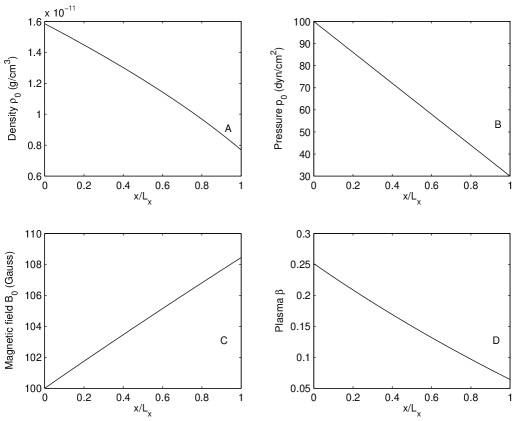
Figure 2: The profiles of the equilibrium quantities plotted against dimensionless $x/L_{x}$ coordinate: density (panel A), pressure (panel B), the magnetic field (panel C) and plasma beta (panel D)

.

4.1 Propagating Alfvén waves

Let us now address the non-linear action of the fast magnetosonic waves, considered in the previous section, on Alfvén waves. We study the weakly non-linear regime. This means that the amplitudes of the fast magnetosonic waves are considered to be large enough to produce significant variations of the environment parameters, which can be felt by propagating Alfvén modes, but too small to affect the Alfvén modes themselves. Hence, the magnetic flux surfaces can still evolve independently. Therefore, as in paper I, the non-linear terms in the equations arising from the advective derivatives $u_{x}\partial b_{y}/\partial x$ and $\left(\rho_{0}+\rho_{1}\right)u_{x}\partial u_{y}/\partial x$ are assumed to be negligible. Under these circumstances the governing set of equations takes the form (see Paper I):

$$\frac{\partial b_{y}}{\partial t}=\left(B_{0}+b_{z}\right)\frac{\partial u_{y}}{\partial z}-\frac{\partial u_{x}}{\partial x}b_{y},$$ (20)

$$\left(\rho_{0}+\rho_{1}\right)\frac{\partial u_{y}}{\partial t}=\frac{B_{0}+b_{z}}{4\pi}\frac{\partial b_{y}}{\partial z}.$$ (21)

These equations describe the parametric influence of fast magnetosonic waves propagating across the magnetic field on Alfvén waves propagating along the field. An analytical solution of Eqs. (20) and (21) is possible for a standing pattern of fast magnetosonic waves, the medium being assumed bounded in the $x$ direction.

Combining Eqs. (20) and (21) we obtain the following second order partial differential equation:

$$\frac{\partial^{2}b_{y}}{\partial t^{2}}+\left[\frac{\partial u_{x}}{\partial x}-\frac{1}{B_{0}+b_{z}}\frac{\partial b_{z}}{\partial t}\right]\frac{\partial b_{y}}{\partial t}+$$

$$+\left(\frac{\partial^{2}u_{x}}{\partial t\partial x}-\frac{1}{B_{0}+b_{z}}\frac{\partial b_{z}}{\partial t}\frac{\partial u_{x}}{\partial x}\right)b_{y}-\frac{(B_{0}+b_{z})^{2}}{4\pi\left(\rho_{0}+\rho_{1}\right)}\frac{\partial^{2}b_{y}}{\partial z^{2}}=0.$$ (22)

Writing

$$b_{y}=h_{y}(z,t)\exp\left[-\frac{1}{2}\int\left(\frac{\partial u_{x}}{\partial x}-\frac{1}{B_{0}+b_{z}}\frac{\partial b_{z}}{\partial t}\right)dt\right],$$ (23)

we obtain

$$\frac{\partial^{2}h_{y}}{\partial t^{2}}+\frac{1}{2}\left[S_{1}(x,t)-S_{2}(x,t)\right]h_{y}-S_{3}(x,t)\frac{\partial^{2}h_{y}}{\partial z^{2}}=0,$$ (24)

where,

$$S_{1}=\frac{\partial^{2}u_{x}}{\partial t\partial x}+\frac{1}{B_{0}+b_{z}}\frac{\partial^{2}b_{z}}{\partial t^{2}},$$ (25)

$$S_{2}=\frac{1}{\left(B_{0}+b_{z}\right)^{2}}\left(\frac{\partial b_{z}}{\partial t}\right)^{2}+\frac{1}{2}\left[\frac{\partial u_{x}}{\partial x}+\frac{1}{B_{0}+b_{z}}\frac{\partial b_{z}}{\partial t}\right]^{2},$$ (26)

$$S_{3}=\frac{(B_{0}+b_{z})^{2}}{4\pi\left(\rho_{0}+\rho_{1}\right)}.$$ (27)

Finally, applying a Fourier analysis with respect to the $z$ coordinate,

$$h_{y}(z,t)=\int\hat{h}_{y}(k_{z},t)e^{ik_{z}z}dk_{z},$$ (28)

and neglecting the second and higher order terms in $\alpha$, we obtain the following Mathieu-type equation:

$$\frac{\partial^{2}\hat{h}_{y}}{\partial t^{2}}+k_{z}^{2}V_{A}^{2}\left[1+\alpha\digamma(x)\cos(\omega_{n}t)\right]\hat{h}_{y}=0,$$ (29)

where

$$\digamma(x)=2\frac{h(x)}{B_{0}}-\frac{r(x)}{\rho_{0}}-v(x)\frac{\omega_{n}}{2k_{z}^{2}V_{A}^{2}}\frac{1}{B_{0}}\frac{dB_{0}}{dx}.$$ (30)

It should be noted that the expression (26) for $S_{2}(x,t)$ consists only of terms of second order and higher in $\alpha$, and so can be neglected directly for the case of weakly non-linear action addressed here.

Equation (29) has a resonant solution when the frequency of the Alfvén mode $\omega_{A}$ is half of $\omega_{n}$:

$$\omega_{A}=k_{z}V_{A}(x)\approx\frac{1}{2}\omega_{n}.$$ (31)

This solution can be expressed as

$${\hat{h}_{y}}(k_{z},t)={\hat{h}_{y}}(k_{z},t=0)e^{{{\left|{\delta}\right|}\over{2\omega_{n}}}t}\left[{\cos}{{\omega_{n}}\over 2}t-{\sin}{{\omega_{n}}\over 2}t\right],$$ (32)

where

$$\delta(x)=\alpha k_{z}^{2}V_{A}^{2}(x)\digamma(x).$$ (33)

The solution has a resonant nature within the frequency interval

$$\left|\omega_{A}-\frac{\omega_{n}}{2}\right|<\left|\frac{\delta}{\omega_{n}}\right|.$$ (34)

Similar expressions have been obtained in the Paper I for a homogeneous medium. In that case, the Alfvén speed is constant and, therefore, the fast magnetosonic waves amplify the Alfvén waves with the same wavelength everywhere. In the case of an inhomogeneous Alfvén speed, the resonance condition (31) implies that the wavelength of the resonant harmonics of the Alfvén waves depends on $x$. This means that the fast magnetosonic waves now amplify Alfvén waves with different wavelengths (but with the same frequency) in different magnetic flux surfaces (i.e., different $x$-values).

4.2 Standing Alfvén waves

When we consider a system that is bounded in the $z$ direction, the boundary conditions along the $z$ axis introduce an additional quantization of the wave parameters. In particular, in this case each spatial harmonic of the Alfvén mode can be represented as

$$\hat{h}_{y}^{m}=\hat{h}_{y}(k_{m},t)\cos(k_{m}z),$$ (35)

where $k_{m}=\pi m/L_{z}$ ($m=1,2,\ldots$) and $L_{z}$ is the characteristic length of the system in the $z$ direction. This then leads to a further localization of the spatial region where the swing transfer of wave energy from longitudinal to transversal oscillations is permitted. The resonant condition (31) implies that

$$k_{m}V_{A}(x_{n,m})\approx\frac{1}{2}\omega_{n}.$$ (36)

Therefore, the resonant areas are concentrated around the points $x_{n,m}$ for which condition (36) holds. Within these resonant areas the longitudinal oscillations damp effectively and their energy is transferred to transversal oscillations with wave numbers $k_{z}=k_{m}$ satisfying the resonant conditions. These resonant areas are localized in space and can be referred to as regions of swing absorption of the fast magnetosonic oscillations of the system. The particular feature of this process is that the energy transfer of fast magnetosonic waves to Alfvén waves occurs at half the frequency of the fast waves.

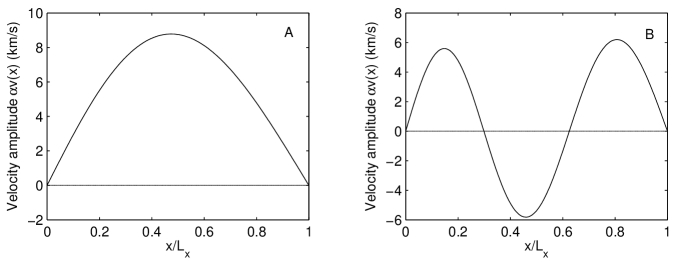
Figure 3: Sample solutions of the standing fast magnetosonic modes. Panel A: zeroth-order harmonic $n=0$, period $T=5.6069$ min., $\alpha=0.015$ ; Panel B: second-order harmonic $n=2$, period $T=1.8514$ min., $\alpha=0.03$

.

5 Numerical study of the problem

In this section we consider in detail the process of swing absorption of fast waves into Alfvén waves. We consider a numerical study of equation (11) subject to the boundary conditions (12). We obtained a numerical solutions of Eqs. (20) and (21) by using the standard Matlab numerical code for solving sets of ordinary differential equations. We study, as an example, the case of a polytropic plasma when both the thermal and magnetic pressures are linear functions of the $x$ coordinate:

$$p_{0}=p_{00}+p_{01}\frac{x}{L_{x}},$$ (37)

$$\rho_{0}=C^{2}\left(p_{00}+p_{01}\frac{x}{L_{x}}\right)^{\frac{1}{\gamma}},$$ (38)

$$B_{0}=\sqrt{h_{00}+h_{01}\frac{x}{L_{x}}},$$ (39)

where, $p_{00}$, $p_{01}$, $h_{00}$, $h_{01}$ and $C$ are constants, and $L_{x}$ denotes the length of the system along the $x$ direction. The pressure balance condition (5) immediately yields

$$p_{01}=-\frac{h_{01}}{8\pi}.$$ (40)

The solution of the wave equation depends on the values of the above set of constant parameters. In general, different equilibrium regimes can be considered including those corresponding to different limits of the plasma ${\beta}$: $\beta\ll 1$, $\beta\approx 1$ and $\beta\gg 1$. However, here we consider the case of the $\beta$ profile shown in Figure 2 (panel D).

$p_{00}$ dyn/cm2	$p_{01}$ dyn/cm2	$h_{00}$ G2	$h_{01}$ G2
100	-70	$10^{4}$	$1.7593\cdot 10^{3}$
$L_{x}$ km	$L_{z}$ km	$C$	$\gamma$
15000	$6.5\cdot L_{x}$	$10^{-6}$	$5/3$

Table 1: Values of the constant parameters used in the calculation of our illustrative solutions. The dimension of $C$ is g^1/2cm^(2-3γ)/2γ/$dyn^{1/2\gamma}$

.

The values of all constant parameters are given in Table 1. We took arbitrary values of parameters, but they are somewhat appropriate to the magnetically dominated solar atmosphere (say the chromospheric network). In Figure 2 corresponding equilibrium profiles of the density (panel A), pressure (panel B), the magnetic field (panel C) and plasma beta (panel D) are shown. In Figure 3 we show the profiles of $\alpha v(x)$ for the standing wave solutions, for two cases with different modal ‘wavelength’. Panels A and B, respectively, correspond to the characteristic frequencies:  $\omega_{0}\approx 1.87\cdot 10^{-2}$ s^-1 (period 5.61 min) and  $\omega_{2}\approx 5.66\cdot 10^{-2}$ s^-1 (period 1.85 min).

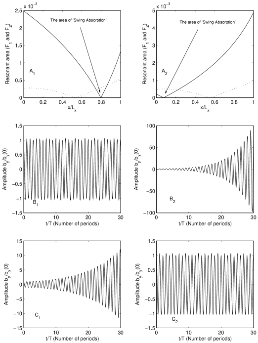
Figure 4: Results of numerical simulations for the standing fast magnetosonic mode, shown on panel A in Figure 3. Panel A₁: the curves of $F_{1}$ (Eq. (42)) (solid line) and $F_{2}$ (Eq. (43)) (dotted line) vs. fractional distance $x/L_{x}$ for the zeroth-order standing fast mode $n=0$ and the standing Alfvén mode with $m=3$; Panel B₁: The numerical solution of the Alfvén mode $m=3$ amplitude at location $x/L_{x}\approx x_{0,4}/L_{x}=0.0767$; Panel C₁: The numerical solution for mode $m=3$ at $x/L_{x}\approx x_{0,3}/L_{x}=0.7967$; Panel A₂: As in panel A₁ for mode $m=4$; Panel B₂: As in panel B₁ for mode $m=4$; Panel C₂: As in panel C₁ for mode $m=4$.

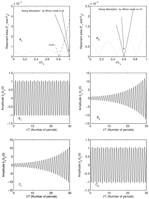
Figure 5: As in Figure 4 for the second-order harmonic of the fast magnetosonic mode shown on Panel B in Figure 3 ($n=2$) and the standing Alfvén with $m=8$ and $m=10$. The numerical solutions respectively are given at distances $x_{1}/L_{x}\approx x_{2,10}/L_{x}=0.6000$ (panels B₁ and B₂), $x_{2}/L_{x}\approx x_{2,8}/L_{x}=0.9933$ (panels C₁ and C₂). Dashed line in panel A₁ is curve of $F_{1}$ (42) corresponding to the mode $m=9$.

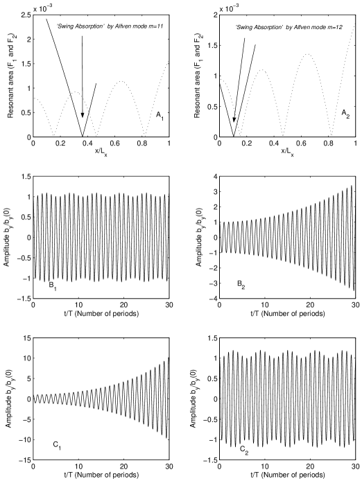
Figure 6: As in Figure 5 for the standing Alfvén modes with $m=11$ and $m=12$ at respective resonant points $x_{1}/L_{x}\approx x_{2,12}/L_{x}=0.1033$ (panels B₁ and B₂), $x_{2}/L_{x}\approx x_{2,11}/L_{x}=0.3633$ (panels C₁ and C₂).

For the configuration described by the equilibrium profiles (37) - (39) the resonant condition (36) yields the areas of swing absorption (located along the $x$ axis) as the solutions of the following equation:

$$\sqrt{\pi}\omega_{n}C\left(p_{00}+p_{01}\frac{x_{n,m}}{L_{x}}\right)^{\frac{1}{2\gamma}}-k_{m}\sqrt{h_{00}+h_{01}\frac{x_{n,m}}{L_{x}}}=0.$$ (41)

In Figure 4 (panels A₁ and A₂) we plot

$$F_{1}=\left|\frac{\omega_{n}}{2}-k_{m}V_{A}\right|$$ (42)

(solid line) and

$$F_{2}=\left|\frac{\delta(x)}{\omega_{n}}\right|$$ (43)

(dotted line) against the normalized coordinate $x/L_{x}$. These curves correspond to the zeroth-order harmonic of the fast magnetosonic mode shown in Figure 3 (panel A) and the standing Alfvén mode with wave numbers $m=3$ (panel A₁) and $m=4$ (panel A₂).

In order to examine the validity of the approximations we made during the analysis of the governing equation (24), we performed a direct numerical solution of the set of equations (20) - (21) and obtained the following results. The Alfvén mode $m=3$ is amplified effectively close to the resonant point $x/L_{x}\approx x_{0,3}/L_{x}=0.7967$. This is shown on panel C₁ of Figure 4. Far from this resonant point, the swing interaction is weaker, as at the point $x/L_{x}\approx x_{0,4}/L_{x}=0.0767$ (panel B₁). For the Alfvén mode $m=4$ we have the opposite picture: the area of ‘swing absorption’ is situated around the point $x_{0,4}$ (see panel B₂, Figure 4) and the rate of interaction between modes decreases far from this area, as at point $x_{0,3}$ (panel C₂, Figure 4). In these calculations we took $\alpha=0.015$.

Similar results are obtained for the fast magnetosonic mode shown in panel B of Figure 3, corresponding to $\alpha=0.03$. In this case, the fast magnetosonic mode effectively amplifies four different spatial harmonics of Alfvén modes, viz. $m=8,10$, $11$ and $12$. There exists one additional resonant point corresponding to the Alfvén mode $m=9$. In panel A₁ of Figure 5 we show the curve of $F_{1}$ for this mode by a dashed line. But, as seen from this plot, the value of $F_{2}$, and consequently the rate of mode amplification $\delta(x)$ in this resonant point, is very small. Therefore the interaction between the modes $n=2$ and $m=9$ is negligible for the considered parameters.

The results of direct numerical calculations for these Alfvén wave harmonics are shown separately in Figures 5 - 6. In Figure 5 (panel A₁), we show the curves corresponding to the mode numbers $n=2$, $m=8$. The calculations were performed at two points $x_{1}/L_{x}\approx x_{2,10}/L_{x}=0.60$ (panel B₁) and $x_{2}/L_{x}\approx x_{2,8}/L_{x}=0.9933$ (panel C₁). In addition, the results of calculations for the mode $m=10$, under the same conditions, are shown in panels A₂,  B₂ and  C₂. It can be seen from these plots that the $m=8$ Alfvén mode is amplified effectively within the resonant area close to the resonant point $x_{2,8}$ (see panel C₁), which corresponds to the harmonic of the standing Alfvén mode with half the frequency. On the other hand, in panels B₁ we see that the action of the fast mode on the Alfvén mode is almost negligible outside the swing amplification area. Correspondingly, we get similar results for the Alfvén modes $m=10$ (Figure 5, panels A₂, B₂ and C₂), and for $m=11$ and $m=12$ (Figure 6) (in the latter case the calculations were done at points $x_{3}/L_{x}\approx x_{2,12}/L_{x}=0.1033$ and $x_{4}/L_{x}\approx x_{2,11}/L_{x}=0.3633$). Again, all these standing Alfvén modes gain their energy from the fast magnetosonic mode $n=2$ only at the resonant points $x_{2,10}$ (for $m=10$, panel B₂ in Figure 5), $x_{2,11}$ (for $m=11$, panel C₁ in Figure 6) and $x_{2,12}$ (for $m=12$, panel B₂ in Figure 6), respectively.

As a conclusion from the above analysis one can claim that the zeroth-order harmonic of the standing fast magnetosonic mode propagating across the magnetic field lines, in the system with characteristic length scales $L_{x}$ and $L_{z}=6.5L_{z}$, can be effectively absorbed only by the standing Alfvén modes with modal numbers $m=3$ and $m=4$ within the resonant areas, respectively, around the point of swing absorption $x_{0,3}$ and $x_{0,4}$. On the other hand, the second-order harmonic of the standing fast mode $n=2$ is absorbed by four harmonics of the standing Alfvén modes, $m=8,10,11,$ and $12$, with respective locations of the resonant areas of swing absorption at $x_{2,8}$, $x_{2,10}$, $x_{2,11}$ and $x_{2,12}$. A similar analysis can be performed for the case of any other equilibrium configuration and corresponding harmonics of the standing fast magnetosonic modes.

6 Discussion

The most important characteristic of swing absorption is that the velocity polarization of the amplified Alfvén wave is strictly perpendicular to the velocity polarization (and propagation direction) of fast magnetosonic waves. This is due to the parametric nature of the interaction. For comparison, the well-known resonant absorption of a fast magnetosonic wave can take place only when it does not propagate strictly perpendicular to the magnetic flux surfaces and the plane of the Alfvén wave polarization. In other words, the energy in fast magnetosonic waves propagating strictly perpendicular (i.e. $k_{\bot}=0$) to the magnetic flux surfaces cannot be resonantly ‘absorbed’ by Alfvén waves with the same frequency polarized in the perpendicular plane. This is because the mechanism of resonant absorption is analogous to the mechanical pendulum undergoing the direct action of an external periodic force. This force may resonantly amplify only those oscillations that at least partly lie in the plane of force. On the contrary, the external periodic force acting parametrically on the pendulum length may amplify the pendulum oscillation in any plane. A similar process occurs when the fast magnetosonic wave propagates across the unperturbed magnetic field. It causes a periodical variation of the local Alfvén speed and thus affects the propagation properties of the Alfvén waves. As a result, those particular harmonics of the Alfvén waves that satisfy the resonant conditions grow exponentially in time. These resonant harmonics are polarized perpendicular to the fast magnetosonic waves and have half the frequency of these waves. Hence, for standing fast magnetosonic waves with frequency $\omega_{n}$, the resonant Alfvén waves have frequency ${\sim}\omega_{n}/2$.

In a homogeneous medium all resonant harmonics have the same wavelengths (see Paper I). Therefore, once a given harmonic of the fast and Alfvén modes satisfies the appropriate resonant conditions (Eqs. (23) and (25) in Paper I), then these conditions are met within the entire medium. Thus, in a homogeneous medium the region where fast modes effectively interact with the corresponding Alfvén waves is not localized, but instead covers the entire system. However, when the equilibrium is inhomogeneous across the applied magnetic field, the wavelengths of the resonant harmonics depend on the local Alfvén speed. When the medium is bounded along the unperturbed magnetic field (i.e. along the $z$ axis), the resonant harmonics of the standing Alfvén waves (whose wavelengths satisfy condition (36) for the onset of a standing pattern) will have stronger growth rates. This means that the ‘absorption’ of fast waves will be stronger at particular locations across the magnetic field. In the previous section we showed numerical solutions of standing fast magnetosonic modes for a polytropic equilibrium ($p_{0}\sim\rho_{0}^{\gamma}$) in which the thermal pressure and magnetic pressure are linear functions of $x$. Further, we performed a numerical simulation of the energy transfer from fast magnetosonic waves into Alfvén waves at the resonant locations, i.e. the regions of swing absorption.

The mechanism of swing absorption can be of importance in a veriety of astrophysical situations. Some possible applications of the mechanism are discussed briefly in the following subsections.

6.1 Swing absorption of global fast magnetosonic waves in the Earth’s magnetosphere

Global standing magnetosonic waves, resulting from the fast MHD waves being reflected between the bow shock or magnetopause and a turning point within the planetary magnetosphere, may be driven by the solar wind (Harrold & Samson, har (1992)). The proposed swing absorption mechanism suggests that these waves may be ‘absorbed’ by shear Alfvén waves with the half frequency, which may form a standing pattern when they are guided along magnetic field lines in the magnetosphere-ionosphere system (reflected by the lower ionosphere at the ends of the magnetic field lines). They are usually described as field line resonances and have been observed as regular ultra-low frequency variations in the magnetic field in the Earth’s magnetosphere and F region flows in the ionosphere (Samson et al. sam (1991), Walker et al. wal (1992)). This standing Alfvén wave pattern may act as an electromagnetic coupling mechanism between the auroral acceleration region of the magnetosphere and the ionosphere (Rankin et al. ran (1993)). The results obtained here may be applied to the particular spatial distribution of the background density and magnetic field of the Earth’s magnetosphere.

6.2 Absorption of p-modes in sunspots

Solar $p$-modes interact strongly with sunspots. Sunspots (and other magnetic field concentrations) scatter and absorb significantly ingoing acoustic modes (see Braun et al. brdulb (1987), bretl (1992); Bogdan et al. bogdetl (1993); Zhang zha (1997)). Understanding the mechanisms leading to the transformation and damping of waves is thus an important issue in sunspot seismology (see Braun braun (1995); Cally et al. caletl (2003)). The $p$-modes split into fast and slow modes (see, for example, Spruit & Bogdan spru (1992); Cally & Bogdan calbog (1993); Bogdan & Cally bogdcal (1997); Cally call (2000)) and these latter modes have a different nature in a  high-$\beta$ plasma. In particular, fast modes (or $\pi$-modes, Cally & Bogdan calbog (1993)) behave similarly to non-magnetized $p$-modes (and they predominantly propagate across the magnetic field lines), while the nature of slow modes is closer to that of Alfvén modes (they mostly travel along the field lines). Further, the damping of incident MHD modes, satisfying local resonant conditions, through the mechanism of resonant absorption has been intensively studied (see, for example, Keppens, Bogdan & Goossens kepbogdgos (1994); Stenuit et al. sten1 (1993), sten2 (1995), 1998a , 1998b ). The mechanism of swing absorption discussed here may also be involved in the damping of incident $p$-modes in sunspots, which accordingly satisfy special resonant conditions (as discussed earlier). Then their energy can be transferred into Alfvén waves and the amplified Alfvén waves may propagate upwards and carry their energy into the chromosphere and corona.

7 Conclusions

We have shown that swing interaction (Zaqarashvili zaq (2001); Zaqarashvili and Roberts 2002a ) may lead to fast magnetosonic waves, propagating across a non-uniform equilibrium magnetic field, transforming their energy into Alfvén waves propagating along the magnetic field. This process differs from resonant absorption. Firstly, the resonant Alfvén waves have only half the frequency of the incoming fast magnetosonic waves. Secondly, the velocity of the Alfvén waves is polarized strictly perpendicular to the velocity and propagation direction of the fast magnetosonic waves. The mechanism of swing absorption can be of importance in the dynamics of the solar atmosphere, the Earth’s magnetosphere, and in astrophysical plasmas generally.

Here we presented the results of a numerical study of the problem, illustrating the process for two particular harmonics of the standing fast modes in a specific equilibrium configuration. Further numerical and theoretical analysis is needed in order to explore the proposed mechanism of swing absorption in the variety of inhomogeneous magnetic structures recorded in observations. Such tasks are to be the subject of future studies.

- (1) Aschwanden, M. 2003, In ‘Turbulence, Waves and Instabilities in the Solar Plasma’, Edited by R. Erdélyi et al., NATO Science Series, Kluwer Academic Publishers, p. 215
- (2) Bogdan, T. J., & Cally, P. S. 1997, Proc. R. Soc. Lond. A, 453, 943
- (3) Bogdan, T. J., Brown, T. M., Lites, B.W., & Thomas, J.H. 1993, ApJ, 406, 723
- (4) Braun, D. C. 1995, In Proc. GONG ’94 ‘Helio- and Astero-Seismology from the Earth and Space’, Edited by R. K. Ulrich, E. J. Rhodes Jr. and W. Dappen, Astronomical Society of the Pacific, San Francisco, California, Vol. 76, p. 250
- (5) Braun, D. C., Duvall, T. L., & LaBonte, B. J. 1987, ApJ, 319, L27
- (6) Braun, D. C., Duvall, T. L., LaBonte, B. J., Jefferies, S.M., Harvey, J. W., & Pomerantz, M. A. 1992, ApJ, 391, L113
- (7) Cally, P. S. 2000, Solar Phys., 192, 395
- (8) Cally, P. S., & Bogdan, T. J. 1993, ApJ, 402, 732
- (9) Cally, P. S., Crouch, A. D., & Braun D.C. 2003, MNRAS, 346, 381
- (10) Chagelishvili, G. D., Rogava, A. D., & Tsiklauri, D. G. 1996, Phys. Rev E, 53, 6028
- (11) Chen, L., & Hasegawa, A. 1974, Phys. Fluids, 17, 1399
- (12) Craik, A. D. D. 1985, Wave Interactions and Fluid Flows, Cambridge University Press
- (13) Galeev, A. A., & Oraevski, V. N. 1962, Sov. Phys. Dokl., 7, 998
- (14) Goldreich, P., & Linden-Bell, D. 1965, MNRAS, 130, 125
- (15) Goossens, M. 1991, In ‘Advances in Solar System - Magnetohydrodynamics’, Edited by E.R. Priest and A.W. Hood, Cambridge University Press, p. 137
- (16) Harrold, B. G., & Samson, J. C. 1992, Geophys. R. L., 19, 1811
- (17) Heyvaerts, J., & Priest, E. R. 1983, A&A, 117, 220
- (18) Hollweg, J. V. 1987, ApJ, 317, 514
- (19) Ionson, J. A. 1978, ApJ, 226, 650
- (20) Keppens, R., Bogdan, T. J., & Goossens, M. 1994, ApJ, 436, 372
- (21) Lord Kelvin (W. Thomson) 1887, Phil. Mag., 24, Ser. 5, 188
- (22) Nakariakov, V. M., Roberts, B., & Murawski, K. 1997, Sol. Phys., 175, 93
- (23) Ofman, L., & Davila, J. M. 1995, J. Geophys.Res., 100, 23427
- (24) Oraevski, V. N. 1983, in Foundations of Plasma Physics, edited by A. A. Galeev and R. Sudan, Nauka, Moscow
- (25) Poedts, S. 2002, In Proc. Euroconference and IAU Colloquium 188 ‘Magnetic Coupling of the Solar Atmosphere’, Santorini, Greece, ESA SP-505, p. 273
- (26) Poedts, S., Goossens, M., & Kerner, W. 1989, Sol. Phys., 123, 83
- (27) Rae, I. C., & Roberts, B. 1982, MNRAS, 201, 1171
- (28) Rankin, R., Harrold, B.G., Samson, J.C., & Frycz, P. 1993, J. Geophys. R., 98, 5839
- (29) Roberts, B. 1981, Solar Phys., 69, 27
- (30) Roberts, B. 1991, In ‘Advances in Solar System Magnetohydrodynamics’, Edited by E.R. Priest and A.W. Hood, Cambridge University Press, p. 105
- (31) Roberts, B. 2002, In ‘Solar Variability: From Core to Outer Frontiers’, Prague, Czech Republic, 9-14 September 2002 (ESA SP-506), p. 481
- (32) Roberts, B. 2004, In Proc. SOHO 13 ‘Waves, Oscillations and Small-Scale Transient Events in the Solar Atmosphere: A Joint View from SOHO and TRACE’, Palma de Mallorca, Spain, (ESA SP-547), p. 1
- (33) Roberts, B., & Nakariakov, V. M. 2003, In ‘Turbulence, Waves and Instabilities in the Solar Plasma’, Edited by R. Erdélyi et al., NATO Science Series, Kluwer Academic Publishers, p. 167
- (34) Rogava, A. D., Poedts, S., & Mahajan S. M. 2000, A&A, 354, 749
- (35) Ryutova, M. P. 1977, In Proc. of XIII Int. Conf. on Ionized Gases, Berlin, ESA, p. 859
- (36) Sagdeev, R. Z., & Galeev A. A. 1969, Nonlinear Plasma Theory, Benjamin, New York
- (37) Samson, J. C., Greenwald, R. A., Ruohoniemi, J. M., Hughes, T. J., & Wallis, D. D. 1991, Can. J. Phys., 69, 929
- (38) Spruit, H. C., & Bogdan, T. J. 1992, ApJ, 391, L109
- (39) Stenuit, H., Poedts, S., & Goossens, M. 1993, Solar Phys., 147, 13
- (40) Stenuit, H., Erdélyi, R., & Goossens, M. 1995, Solar Phys., 161, 139
- (41) Stenuit, H., Keppens, R., & Goossens, M. 1998, A&A, 331, 392
- (42) Stenuit, H., Tirry, W. J., Keppens, R., & Goossens, M. 1998, A&A, 342, 863
- (43) Walker, A. D. M., Ruohoniemi, J. M., Baker, K. B., Greenwald, R. A., & Samson, J. C. 1992, J. Geophys. Res., 97, 12187
- (44) Zaqarashvili, T. V. 2001, ApJ Letters, 552, L81
- (45) Zaqarashvili, T. V., & Roberts, B. 2002a, Phys. Rev. E, 66, 026401 (Paper I)
- (46) Zaqarashvili, T. V., & Roberts, B. 2002b, In ‘Solar Variability: From Core to Outer Frontiers’, Prague, Czech Republic, 9-14 September 2002 (ESA SP-506), p. 79
- (47) Zaqarashvili, T. V., Oliver, R., & Ballester, J. L. 2002, ApJ, 569, 519
- (48) Zaqarashvili, T. V., Oliver, R., & Ballester, J. L. 2004, In Proc. SOHO 13 ‘Waves, Oscillations and Small-Scale Transient Events in the Solar Atmosphere: A Joint View from SOHO and TRACE’, Palma de Mallorca, Spain, (ESA SP-547), p. 193
- (49) Zhang, H. 1997, ApJ, 479, 1012