Structure in the polarized Galactic synchrotron emission, in particular “depolarization canals”

The polarized component of the diffuse radio synchrotron emission of our Galaxy shows structure, which is apparently unrelated to the structure in total intensity, on many scales. The structure in the polarized emission can be due to several processes or mechanisms. Some of those are related to the observational setup, such as beam depolarization – the vector combination and (partial) cancellation of polarization vectors within a synthesized beam –, or the insensitivity of a synthesis telescope to structure on large scales, also known as the ’missing short spacings problem’. Other causes for structure in the polarization maps are intrinsic to the radiative transfer of the emission in the warm ISM, which induces Faraday rotation and depolarization.

We use data obtained with the Westerbork Synthesis Radio Telescope at 5 frequencies near 350 MHz to estimate the importance of the various mechanisms in producing structure in the linearly polarized emission. In the two regions studied here, which are both at positive latitudes in the second Galactic quadrant, the effect of ’missing short spacings’ is not important. The properties of the narrow depolarization ’canals’ that are observed in abundance lead us to conclude that they are mostly due to beam depolarization, and that they separate regions with different rotation measures. As beam depolarization only creates structure on the scale of the synthesized beam, most of the structure on larger scales must be due to depth depolarization. We do not discuss that aspect of the observations here, but in a companion paper we derive information about the properties of the ISM from the structure of the polarized emission.

1 Introduction

The omnipresent cosmic rays in the Milky Way, spiraling in the Galactic magnetic field, provide a synchrotron radio background which is partially polarized. This radiation propagates through the warm ionized interstellar medium (ISM) and is modulated by it. This makes observations of the polarized continuum radio background a valuable tool for studies of the warm ISM and the Galactic magnetic field.

Generally, observations of the polarized synchrotron emission of the Galaxy show small-scale structure in polarized intensity $P$ or polarization angle $\phi$ uncorrelated with structure in total intensity $I$ (e.g. Wieringa et al. 1993, Duncan et al. 1999, Gray et al. 1999, Gaensler et al. 2001, Uyanıker and Landecker 2002 for the Milky Way; Horellou et al. 1992, Berkhuijsen et al. 1997 for M51; Shukurov and Berkhuijsen 2003, Fletcher et al. 2004 for M31). The lack of correlation between $P$ and $I$ indicates that the structure in polarization is not exclusively due to intrinsic structure in synchrotron emission. Instead, the fluctuations in polarization angle are explained in terms of Faraday rotation of the synchrotron radiation that impinges on the magneto-ionic medium of the ISM relatively close to the Sun (Burn 1966). Multi-frequency polarimetry of the synchrotron emission allows determination of the Faraday rotation measure $RM\propto\int n_{e}B_{\parallel}\,ds$, which depend on electron density $n_{e}$, magnetic field parallel to the line of sight $B_{\parallel}$ and path length $ds$. Thus, study of RMs enables the study of the structure and electron-density-weighted strength of the Galactic magnetic field.

However, whereas Faraday rotation can explain the variation in polarization angle, it does not provide an explanation for the structure in polarized intensity $P$. Although the lack of zero-baseline visibilities in some interferometric observations could produce structure in $P$ from structure in $\phi$, this would leave the structure in $P$ in absolutely calibrated single-dish observations unaccounted for. Therefore, depolarization must also contribute to structure in polarized intensity and polarization angle. Detailed analysis of the different depolarization mechanisms yield unique information on the magnetic field.

Two different approaches to the description of depolarization mechanisms can be found in the literature: one which is based on the physical processes that produce the depolarization, and another that makes a geometrical distinction between effects in depth and in angle. In this paper, we use the latter, which is more convenient for our purpose. We will first discuss the physical processes causing depolarization, and then describe how these are treated here. For extensive treatments of the depolarization processes see e.g. Gardner and Whiteoak (1966), Burn (1966), or Sokoloff et al. (1998).

• Wavelength independent depolarization is due to turbulent magnetic fields in the ISM. Cosmic rays in a turbulent magnetic field emit synchrotron radiation with varying polarization angle. Therefore, superposition of the polarization vectors along the line of sight and across the telescope beam results in partial depolarization of the emission, independent of wavelength. No Faraday rotation is involved.

• Differential Faraday rotation occurs if a medium contains thermal and relativistic electrons and a (partly) regular magnetic field. Synchrotron radiation emitted at different distances along the line of sight undergo different amounts of Faraday rotation. This is a one-dimensional (along the line of sight), wavelength dependent depolarization effect.

• Internal Faraday dispersion is the depolarization in a turbulent synchrotron-emitting magneto-ionic medium. It is a combination of the two effects described above, but it also involves depolarization within the telescope beam. Variation in intrinsic polarization angle and in Faraday rotation, which occur both along the line of sight and across the telescope beam, cause depolarization of the radiation.

Here, it is more convenient to divide these depolarization mechanisms in those operating along the line of sight and those perpendicular to the line of sight, regardless of the physical process causing the depolarization. The latter mechanism is called beam depolarization (Gray et al. 1999, Gaensler et al. 2001, Landecker et al. 2001, which is a result of vector averaging for neighboring directions within the same telescope beam. Depolarization along the line of sight is depth depolarization (Landecker et al. 2001, Uyanıker and Landecker 2002, referred to as front-back depolarization by Gray et al. 1999), and is a one-dimensional addition of polarization vectors, assuming an infinitely narrow telescope beam. Depth depolarization is a combination of differential Faraday rotation, internal Faraday dispersion and depolarization due to variations of the intrinsic polarization angle along the line of sight.

In this paper, we discuss various processes that can produce structure in $P$, and we use several multi-frequency datasets obtained with the Westerbork Synthesis Radio Telescope (WSRT) to gauge their importance. The influence of missing short spacings and of depolarization mechanisms on the data is estimated, as well as the importance of beam depolarization. A discussion of the effects of depth depolarization is given in a companion paper (Haverkorn et al. 2004).

In Sect. 2 we summarize the relevant parameters of the Westerbork polarization observations that will be used to estimate the importance of the various effects that contribute to the structure in $P$. In Sect. 3 the rôle of missing short spacings in interferometer measurements is estimated, and we discuss how the resulting images can be affected. Section 4 presents a discussion on the origin of depolarization canals in polarized intensity. Finally, the conclusions are stated in Sect. 5.

2 The observations

	Auriga	Horologium
(l,b)	(161∘, 16∘)	(137∘, 7∘)
size	7∘$\times$9∘	7∘$\times$7∘
FWHM	5.0′$\times$6.3′	5.0′$\times$5.5′
pointings	5$\times$7	5$\times$5
Noise (mJy/bm)	$\sim$ 4 (0.5 K)	$\sim$ 5 (0.7 K)
1 mJy/bm =	0.127 K	0.146 K
(at 350 MHz)
bandwidth	5 MHz	5 MHz
frequencies	341, 349, 355, 360, 375 MHz

Table 1: Details of the WSRT polarization observations in the constellations Auriga and Horologium.

We use Westerbork Synthesis Radio Telescope (WSRT) observations around 350 MHz in two fields in the constellations Auriga and Horologium, which were described in detail by Haverkorn et al. (2003a, 2003b). Some details of the observations are described in Table 1.

Fig. 1 shows the RM distribution in the Auriga (left) and Horologium (right) fields as circles, superposed on polarized intensity in grey scale. The structure in $P$ is uncorrelated with total intensity $I$. The RMs were derived from $\phi=\phi_{0}+RM\lambda^{2}$, where $\phi_{0}$ is the intrinsic polarization angle at $\lambda=0$. Depolarization mechanisms alter Stokes $Q$ and $U$, and can destroy the linear $\phi(\lambda^{2})$-relation, in which case the determined $RM$ will not have its simple meaning, viz. $\int n_{e}B_{\parallel}ds$ (Sokoloff et al. 1998). Therefore, we only show RM values at positions where (a) the reduced $\chi^{2}$ of the linear $\phi(\lambda^{2})$-relation $\chi^{2}_{red}<2$, and (b) the polarized intensity averaged over frequency $\left<P\right>>20$ mJy/beam ($\sim 4$ to 5 $\sigma$). The upper limit of $\chi^{2}=2$ is chosen to allow for slight non-linearity due to depolarization.

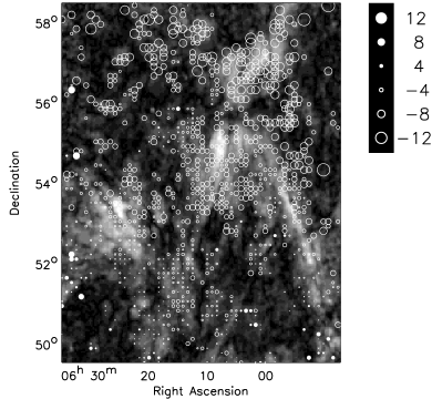
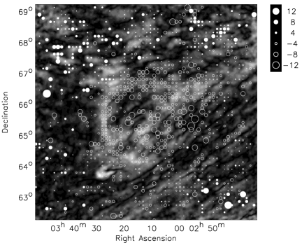
Figure 1: Rotation measure maps of the regions in Auriga (left) and in Horologium (right), superimposed on polarized intensity in grey scale where the maximum is 90 mJy/beam for Auriga and 110 mJy/beam for Horologium. Rotation measures are denoted by white circles, where filled circles are positive $RM$s. The diameter of the symbol represents the magnitude of $RM$, and the scaling is given in rad m^-2. Only $RM$s for which $\langle P\rangle\geq 5\sigma$ and reduced $\chi^{2}$ of the linear $\phi(\lambda^{2})$-relation $<2$ are shown, and only every second independent beam.

3 The effect of missing short spacings in aperture synthesis observations

In aperture synthesis observations, structure on large angular scales is not well represented because visibilities cannot be measured on baselines smaller than the diameter of the primary elements. (Also single-dish observations miss information about structure on scales larger than the mapped region, and missing flux must be added from absolutely calibrated polarization maps.) The shortest baseline of the WSRT is 36m, so that at 350 MHz, structure on angular scales larger than about a degree is not adequately measured. The proper way to correct for this undetectable large-scale structure is to observe the same region at the same frequencies with a single-dish telescope with absolute intensity scaling and add these large-scale data to the interferometer data (see Stanimirovic (2002) for methods of data addition, and Uyanıker et al. (1998) who have first done this for diffuse polarization data). However, for the WSRT at 350 MHz this is not possible, as there is no instrument of suitable size operating at these frequencies.

In the data reduction process of the WSRT, the lack of information on scales larger than about a degree is dealt with by setting the average value of measured intensities on the scale of the whole field to zero. For a strong source this will result in an image which has a bowl-like depression around the source, but for approximately uniform diffuse emission, it produces a more or less constant offset. In the case of polarimetry, this means that the average Stokes $Q$ and $U$ components are set to zero. So in each observed $Q$ and $U$ map there may be constant offsets $Q_{0}$ and $U_{0}$ that have to be added to the observed $Q$ and $U$ to obtain the real linearly polarized signal on the sky. Since the large mosaics are produced from several tens of pointings, each of which can have its own offsets, the offsets can vary over a mosaic.

3.1 The effect of offsets on polarized intensity and rotation measure

The presence of offsets can create spurious small-scale structure in observed $P$. In particular, offsets can create additional depolarization canals (see Sect. 4) as shown in Uyanıker et al. (1998). Fig. 2 shows an example of the effect of offsets on $Q$ and $U$. The left plot gives a simple one-dimensional model of a change in polarization angle, which causes small-scale structure in the distribution of $Q$ and $U$, but not in $P$ (center plot). The right plot shows the response of an interferometer: the average $Q$ and $U$ over the field are subtracted from the signal on the sky. $P_{obs}$ which is computed from $Q_{obs}$ and $U_{obs}$ does show apparent structure on small scales, although in reality it does not have that structure.

Figure 2: Illustration of how offsets can cause small-scale structure in $P$. Left: an model polarization angle distribution in one dimension, where $P$ is assumed constant. Center: small-scale structure in $Q$ (solid line) and $U$ (dashed line) corresponding to the change in polarization angle, while $P$ (dotted line) remains constant. Right: the interferometer response to this distribution, where $P$ does show apparent structure.

Figure 3: The effect that offsets have on apparent RMs. Top: hypothetical polarization vectors at 3 adjacent positions in the sky for three values of true RM, at 5 wavelengths denoted 1 to 5. Center: results after subtracting offsets determined from the situation in the top panel, showing how the offsets can destroy the linear $\phi(\lambda^{2})$-relation. Bottom: 4 estimates of $\Delta\phi$ for each wavelength step $\Delta\lambda^{2}$, which gives the apparent $RM=\Delta\phi/\Delta\lambda^{2}$ as the slope of a linear fit of $\phi$ to $\lambda^{2}$.

Furthermore, if undetected offsets are present in the data, the polarization angle computed from the detected $Q$ and $U$ will, in general, not show a linear dependence on $\lambda^{2}$. Therefore, the fitted RM will then differ from the real one. Although in interferometer observations the Stokes $Q$ and $U$ emission can be separated in (observable) small-scale structure and (unobservable) large-scale structure, this is in general not true for the rotation measure, due to the complicated non-linear relation between intensity at different frequencies and $RM$. Therefore, large-scale structure or constant non-zero RMs can be observed as long as small-scale structure in RM is present as well to cause sufficient structure in $Q$ and $U$ on small scales.

A simple example of how offsets may destroy the linear $\phi(\lambda^{2})$-relation and result in erroneous determinations of $RM$ is given in Fig. 3. Six plots in the $(Q,U)$-plane are shown, each with five polarization vectors ${\mathbf{P}}=P\exp(-2i\phi)$. Each vector refers to one of the five wavelengths, which are equally spaced in $\lambda^{2}$, and are numbered according to increasing $\lambda^{2}$. The upper three plots give a hypothetical situation of three values of true RM at three adjacent positions, where the vectors denote the true polarization. All three $RM$s are chosen to be positive, and the value of $RM$ in the left plot is doubled and tripled in the central and right hand plot, respectively. Of these three plots, the $Q$ and $U$ values averaged over the three positions for each band separately were subtracted after which the polarization vectors in the lower plots were obtained. Below these are shown the resulting values of $\Delta\phi$ between two adjacent wavelengths, which gives the apparent $RM=\Delta\phi/\Delta\lambda^{2}$. The linear $\phi(\lambda^{2})$-relation is thoroughly destroyed, and the apparent RM deviates from the true $RM$.

The fact that offsets can create structure in $P$ and prohibit reliable $RM$ determinations has to be given serious consideration in all interferometer observations with missing short spacings. We will estimate the importance of offsets in our observations in the next Section.

3.2 The importance of offsets in the observations

($\delta$)	Auriga
56.2∘	3.76	3.11	2.78	2.28	3.14
55.0∘	3.73	3.64	3.11	2.68	3.15
53.7∘	2.94	2.47	1.51	1.82	3.34
52.5∘	1.99	1.88	1.90	2.00	2.82
51.2∘	2.60	1.87	1.93	2.21	2.37
50.0∘	2.26	1.99	1.79	2.46	2.80
48.7∘	3.09	2.74	2.57	2.52	3.32
	96.6∘	94.6∘	92.5∘	90.5∘	88.4∘	($\alpha$)
($\delta$)	Horologium
68.5∘	2.19	2.59	1.58	3.12	2.71
67.3∘	2.68	2.01	1.83	1.57	1.66
66.0∘	4.42	1.74	1.96	2.04	2.41
64.8∘	2.72	1.84	1.80	1.94	2.16
63.5∘	2.35	1.78	1.85	1.32	1.91
	54.4∘	51.1∘	48.0∘	44.9∘	41.9∘	($\alpha$)

Table 2: Width of $RM$ distribution for each pointing in Auriga (top) and Horologium (bottom). The numbers denote $\sigma_{\scriptscriptstyle\rm RM}$ in rad m^-2, for the pointings given.

Figure 4: $RM$ distributions in separate pointings. The plots show the central row of pointings in the Auriga region. Dotted lines are Gaussian fits to the data, and the fitted $\sigma_{RM}$ are given above the plot.

The offset in each of the pointings of a mosaic depends on the spread in RM in that pointing, see Appendix A. Therefore, we determined $\sigma_{\scriptscriptstyle\rm RM}$ for each pointing in the two mosaics. The values of $\sigma_{\scriptscriptstyle\rm RM}$ for each pointing position in Auriga and Horologium are given in Table 2, while Fig. 4 shows an example of the $RM$ distributions in the central row of pointings in the Auriga field.

For polarized radiation traveling through a non-emitting Faraday screen with a Gaussian random distribution of $RM$s, offsets can be described as (see Appendix A)

$$Q_{0} = A\left[\cos(2\phi_{0})-\frac{1}{\sqrt{\pi}}\sin(2\phi_{0})\;F\right]$$ (1)

$$U_{0} = A\left[\sin(2\phi_{0})-\frac{1}{\sqrt{\pi}}\cos(2\phi_{0})\;F\right]$$ (2)

$$\mbox{where}\;F = \int_{0}^{\sqrt{2}\mbox{$\sigma_{\scriptscriptstyle\rm RM}$}\lambda^{2}}\mbox{e}^{t^{2}}dt\;\;\;\mbox{and}\;\;\;A=P_{0}\mbox{e}^{-2\mbox{$\sigma_{\scriptscriptstyle\rm RM}$}^{2}\lambda^{4}}$$

and offsets are assumed constant over the pointing, with $\phi_{0}$ the intrinsic polarization angle and $P_{0}$ the initial polarized intensity. This confirms that high RM dispersion randomizes any uniform polarized background so that no large-scale components in $Q$ and $U$ remain. Fig. 5 displays the offsets as calculated from Eqs. (1) and (2) for each pointing. The solid and dashed lines denote the theoretical $Q_{0}$ and $U_{0}$ respectively, the symbols show the $\sigma_{\scriptscriptstyle\rm RM}$ in the Auriga field (diamonds) and in the Horologium field (squares). As offsets also depend on $\phi_{0}$, the figure shows minimal offsets (for $\phi_{0}=10\mbox{${}^{\circ}$}$, left) and maximal offsets (for $\phi_{0}=80\mbox{${}^{\circ}$}$, right). The symbols denote the $\sigma_{RM}$ for pointings in the Auriga field (diamonds) and Horologium field (squares).

Figure 5: Missing large-scale structure in $Q$ (solid line) and $U$ (dashed line) for a Faraday screen with a Gaussian RM distribution with width $\sigma_{RM}$ and $P_{0}=1$, assuming that the offsets are constant over the field. Diamonds denote $\sigma_{RM}$ observed in the pointings of the Auriga field, squares are the pointings of the Horologium field. Offsets depend on the intrinsic polarization angle $\phi_{0}$, shown are the best- and worst-case scenario for $\phi_{o}=10\mbox{${}^{\circ}$}$ (left) and $\phi_{0}=80\mbox{${}^{\circ}$}$ (right).

In the best case ($\phi_{0}=10\mbox{${}^{\circ}$}$), no pointings in Auriga and one pointing in Horologium have offsets exceeding 20%, which corresponds to an error in polarization angle $\varepsilon_{\phi}$ of 10%. In the worst case ($\phi_{0}=80\mbox{${}^{\circ}$}$), 3 pointings in Auriga (out of 35) and 9 in Horologium (out of 25) allow offsets above 20%. However, only one pointing (in Horologium) would allow offsets higher than 27% ($\varepsilon_{\phi}=14$%). Therefore, if our observations result from a uniformly polarized background viewed through a Faraday-modulating screen, the $\sigma_{RM}$ in most pointings in our fields is so large that missing large-scale structure leads to an error in polarization angle of less than 10%.

Figure 6: The influence of offsets on reduced $\chi^{2}$ in a subfield of Auriga. Left: reduced $\chi^{2}$ distribution of linear $\phi(\lambda^{2})$-relation with best-fit offsets against values of reduced $\chi^{2}$ without offsets. Right: distribution of reduced $\chi^{2}$ with computed offsets (dotted line) and without offsets (solid line).

The magnitude of the offsets can also be estimated from the variation of observed polarization angle $\phi$ with wavelength. The observations show that $\phi$ does not perfectly follow the linear relation $\phi=\phi_{0}+RM\lambda^{2}$, as one would expect for pure Faraday rotation. Offsets in $Q$ and/or $U$ can cause deviations in the linear $\phi(\lambda^{2})$-relation, so we estimated in both fields the offsets that would minimize the observed non-linearities in the $\phi(\lambda^{2})$-relation.

For this, subfields of $\sim 1\mbox{${}^{\circ}$}\times 1\mbox{${}^{\circ}$}$ were selected around a pointing center. A large-scale constant $Q_{0}$ and/or $U_{0}$, independent for each frequency, were added to the data to minimize the $\chi^{2}$ of the $\phi(\lambda^{2})$-relation. Resulting offset values in some subfields with a magnitude of the same order as $P$ in that field, which decreased the average $\chi_{red}^{2}$ by a factor of two. However, Fig. 6 shows the distribution of individual reduced $\chi^{2}$ values per beam for a typical pointing in the Auriga field. The left plot shows reduced $\chi^{2}$ values computed with offsets against reduced $\chi^{2}$ without offsets. In the right hand panel, the histograms of $\chi^{2}$ without (solid line) and with offsets (dotted line) are given. Offsets only cause a decrease in $\chi^{2}$ in 52% of the beams, although the average $\chi^{2}$ diminishes. In other pointings, this percentage ranges from 49% to 71%. Therefore, the computed offsets do not give a real improvement of the data, and cannot be considered real missing large-scale components. Of course, this argument assumes that offsets are the only agents distorting the linear $\phi(\lambda^{2})$-relation, while depolarization mechanisms can yield non-linearity too. In addition, it assumes that the offsets are constant over the subfield considered, which may not be true either. Probing smaller subfields is no solution for this problem as the number of data points becomes too small with respect to the number of free parameters.

A third argument against dominant offsets in the data is the high quality of the determination of $RM$, i.e. a linear $\phi(\lambda^{2})$-relation with a low $\chi^{2}$. Of all pixels with high enough polarized intensity ($\left<P\right>>20$ mJy/beam), $\sim$ 70% (in Auriga) and $\sim$ 62% (in Horologium) has a reduced $\chi^{2}<2$. If offsets of the same order of the data would exist, $RM$s could not be so well-determined over such a large part of the fields. For ideal data with constant $P$, random offsets cause a $\chi^{2}>2$ if the offsets are larger than $\sim$ 8%.

Finally, models of depolarization in a synchrotron-emitting and Faraday-rotating medium, which are presented in a companion paper (Haverkorn et al. 2004a), do not show average $Q$ or $U$ values $\ga 10$ mJy/beam (2$\sigma$).

From the large $\sigma_{\scriptscriptstyle\rm RM}$, the good quality of the $RM$ determinations, the depolarization models, and from solving for offsets that minimize $\chi^{2}$, we conclude that the presence of considerable undetected large-scale structure due to the missing short spacings is unlikely.

This conclusion can also be checked with absolutely calibrated polarized intensity maps at 408 MHz by Berkhuijsen and Brouw (1963). This frequency is close enough to 350 MHz to allow comparison, although the polarized intensity at 408 MHz is expected to be slightly higher because the polarization horizon is further away at this frequency. We have smoothed our data to the 2^∘ FWHM of Berkhuijsen and Brouw, and derived any missing large-scale structure by comparing the two data sets. The polarized brightness temperatures at 408 MHz at the positions of the Auriga and Horologium fields are 1.8 K and 2.7 K, respectively. Using a power law spectral index of 2.7, this corresponds to 2 K and 3 K at 350 MHz. The polarized brightness temperatures derived from the smoothed data are 0.07 K and 0.12 K, respectively. Converting from Kelvin to Jansky per beam (see Table 1) and taking into account that offsets in $Q$ and $U$ are on average a factor $\sqrt{2}$ smaller than those in $P$, this means that any missing large-scale components in Stokes $Q$ and $U$ are smaller than 10.6 mJy beam^-1 for the Auriga region, and 13.7 mJy beam^-1 for Horologium. For both fields, this corresponds to about 2 to 3 signal-to-noise in $Q$ and $U$, although it is not known what the influence of the difference in polarization horizon is. We conclude that these data are not in disagreement with our conclusion that missing large-scale structure does not play a major role in these observations.

Therefore, the structure in polarized intensity must be due wholly to depolarization mechanisms. For a pure Faraday screen the only kind of depolarization that is possible is beam depolarization, because the observed values of $RM$ imply that bandwidth depolarization is not important, while depth depolarization requires that the rotating medium emits as well. However, beam depolarization can only explain structure in $P$ on beam-size scales. Therefore we are led to consider the more realistic situation in which we observe a polarized background that is modulated by a layer that both causes Faraday rotation, and emits synchrotron radiation. Note that the argument which limits the importance of offsets through the width of the distribution of observed $RM$s applies equally to a pure Faraday rotating screen and to a rotating and emitting screen.

The only way in which offsets could play a rôle is if there were a layer in front of the rotating and emitting screen which emits polarized radiation that is constant over the primary beam of our observations. A foreground-offset decreases the degree of polarization with a constant factor and can contribute a constant $RM$ component which cannot be derived from the data. However, a uniformly polarized foreground cannot influence the width of observed $RM$ distribution or induce small-scale depolarization. Judging from earlier single-dish data of $RM$ in the regions of the Auriga and the Horologium region (Bingham and Shakeshaft 1967, Spoelstra 1984), we conclude that a possible undetected $RM$ component on scales $\ga 1\mbox{${}^{\circ}$}$, if present at all, must be very small.

4 Depolarization canals

A conspicuous feature in the observed polarized intensity is the presence of one-dimensional filament-like structures of low polarized intensity $P$. These so-called depolarization canals have been observed in many diffuse polarization observations (Wieringa et al. 1993, Duncan et al. 1999, Gray et al. 1999, Uyanıker et al. 1998, Gaensler et al. 2001). Two characteristics of the canals in our observations (and in others as far as we could judge from figures) are (1) the canals are one beam wide, and (2) the polarization angle changes across the canal by 90^∘(Haverkorn et al. 2000). This characteristic behavior can be explained by two mechanisms:

1. The canals can denote a boundary between two regions which each have approximately constant polarization angle, but between which there is a difference in polarization angle of $\Delta\phi=(n+1/2)180\mbox{${}^{\circ}$}$ ($n=0,1,2,\ldots$) will cause almost total depolarization through vector addition, if the polarized intensities on either side of the boundary are essentially identical (Haverkorn et al. 2000). The resulting canal is, by definition, one beam wide.

2. A medium containing a uniform magnetic field, thermal electrons and cosmic-ray electrons depolarizes polarized radiation by means of differential Faraday rotation. In this case, the observed polarized intensity is

   $$P=P_{0}\;\left|\frac{\sin(2\,RM\,\lambda^{2})}{2\,RM\,\lambda^{2}}\right|$$ (3)

   (Burn 1966, Sokoloff et al. 1998), where $P_{0}$ is the polarized intensity observed at $\lambda\rightarrow 0$. A linear gradient in $RM$ would produce long narrow depolarization canals at a certain value $RM_{c}$ where $2\,RM_{c}\,\lambda^{2}=n\pi$. Across every null in the sinc-function, the polarization angle changes by 90^∘.

We will attempt to estimate the importance of each of the two mechanisms in our observations.

4.1 Frequency dependence of canals

If the canals are due to beam depolarization, there are two extreme possibilities for the origin of the angle change $\Delta\phi=(n+1/2)\;180\mbox{${}^{\circ}$}$: it can be due to either an RM change across a canal of $(n+1/2)\;180\mbox{${}^{\circ}$}/\lambda^{2}$, or to an intrinsic angle difference of $\Delta\phi_{0}=(n+1/2)\;180$^∘. These two extremes cannot be distinguished from observations at a single frequency. However, one would expect $P$ in the canals to vary with frequency if the RM changes across a canal, while the depth of a canal should be constant for a $\Delta\phi_{0}$. If, on the other hand, the canals are caused by differential Faraday rotation, $P$ in a canal should change with frequency according to Eq. (3).

Figure 7: Frequency dependence of the depth of the canals, in the Auriga region (top) and Horologium region (bottom). $P$ is the average over all canal-pixels, and in each plot the canals were defined in an other frequency band, at 341, 349, 355, 360, and 375 MHz from left to right. The prediction for $P(\lambda^{2})$ if all canals were caused by beam depolarization due to a change in $RM$ is shown in dashed lines, from bottom to top for $\Delta RM\approx$ 2.1, 6.3 rad m^-2 (i.e. $\Delta\phi=90\mbox{${}^{\circ}$},270\mbox{${}^{\circ}$}$). The prediction for $P(\lambda^{2})$ if the canals were caused by differential Faraday rotation are shown dotted for $2RM_{c}\lambda^{2}=n\pi$ for $n=1,3$ and 5.

We have tested the frequency dependence of the depth of the canals as follows. Canals are defined as sets of “canal-pixels”. A pixel is defined as a “canal-pixel” if the polarized intensity is low ($P<$ 2 times rms noise) and $P$ on diametrically opposed sides of that pixel, one beam away, is high ($P>5$ times rms noise). The high-$P$ pixels surrounding the canal-pixel can be oriented horizontally, vertically or diagonally. No further assumptions regarding the length of canals are made; therefore a single pixel with low $P$ that is no part of a canal but is surrounded by high $P$ pixels, is also defined to be a canal-pixel.

Sets of canal-pixels are evaluated for each frequency separately, so that five sets of canal-pixels result. The average $P$ in each set of canal-pixels is computed at all frequencies. In Fig. 7, we plot the average values of $P$ against $\lambda^{2}$ for the five sets of canal-pixels (where canals are defined at one of the frequencies) in the Auriga and Horologium regions. In each panel in Fig. 7, i.e. for each frequency, and both in Auriga and Horologium, the wavelength in which the canals are selected has the lowest average $P$, with $P$ increasing with $|\Delta\lambda^{2}|$, i.e. the canals decrease in depth at the other wavelengths. This rules out the possibility that the canals are caused by a change in intrinsic angle, confirming the conclusion from the non-detection of $I$ that the background polarized intensity is smooth.

The dashed lines show the predictions of $P(\lambda^{2})$ for canals that are caused by beam depolarization, and are due to a change in $RM$ (with $\Delta RM$ = 2.1 and 6.3 rad m^-2, respectively). The dotted lines in Fig. 7 denote the prediction of the polarization angle if the canal is caused by differential Faraday rotation, from Eq. 3). Both predictions have arbitrary polarized intensities. Therefore, the scaling of the models contains no physical information, and is adjusted to fit the data.

The accuracy of the model predictions can be judged by the shape of the predicted lines, which is typical of the responsible depolarization process. Furthermore, the same scaling should be used for each frequency. Judging solely from the shape of the lines, the prediction of differential Faraday rotation seems to make a fit somewhat better than that of beam depolarization, but not by much. This is not totally unexpected, because it is probable that a combination of both processes is at work in the majority of pixels.

4.2 $RM$ and $\Delta RM$ values in canals

Figure 8: Distribution of $\Delta RM_{c}$ across canals and the absolute $RM_{c}$ at the canal position (as estimated from its neighbors). Canals are defined at frequencies 341, 349, 355, 360, and 375 MHz from left to right. Top panels show the Auriga region and bottom panels the Horologium region. Only $RM_{c}$ values where $\chi^{2}_{red}<2$ and $P>20$ mJy/beam are used. In the $\Delta RM_{c}$ plots, dotted vertical lines are $\Delta RM_{c}$ values where $\Delta\phi$ across a canal would be $\pm 90$^∘, $\pm 270$^∘ or $\pm 450$^∘. In the $RM_{c}$ plots, the dotted vertical lines are values where $2RM_{c}\lambda^{2}=n\pi$.

Canals due to beam depolarization are caused by a specific change in $RM$ across a canal $\Delta RM_{c}=(n+1/2)\pi/\lambda^{2}$. On the other hand, canals caused by differential Faraday rotation are determined by a specific absolute $RM_{c}=n\pi/(2\lambda^{2})$. With the sets of canal-pixels defined in the previous subsection, we define $\Delta RM=RM_{1}-RM_{2}$, where 1 and 2 are high-$P$ pixels on opposite sides of the canal. Then the RM at the canal-pixel is estimated as $RM=(RM_{1}+RM_{2})/2$. The observed distributions of $\Delta RM$ and $RM$ are shown in Fig. 8. Both $\Delta RM$ and $RM$ distributions show peaks at the values that will produce canals, and the observations do not show perfect agreement with either of them. Note that canals with angle changes $\Delta\phi\la 90$^∘ have accompanying $\Delta RM$s or $RM$s slightly different from canals with $\Delta\phi=90$^∘  and therefore broaden the peaks. Noise in $RM$ has the same effect.

4.3 Position shift of the canals with frequency

Differential Faraday rotation causes total depolarization at all positions where $RM=RM_{c}$. This means that depolarization not necessarily creates narrow one-dimensional canals, but could also produce patches of $RM=RM_{c}$ that are larger than one beam. The easiest way to explain one-dimensional canals in this picture is to assume a gradient in $RM$, so that the $RM$ stays constant over a certain length perpendicular to the gradient, and a one-dimensional canal is formed. But at 375 MHz, the canal will form at positions where $RM_{c}$ = 2.46 rad m^-2  while at 341 MHz it forms where $RM_{c}$ = 2.02 rad m^-2. If we assume typical gradients of 1 rad m^-2 per degree, similar to the large-scale gradient observed in the Auriga region, this indicates that the canal should move with position over $\sim$ 5 beams from 341 MHz to 375 MHz. Instead, canals move at maximum 3 pixels from 341 to 375 MHz, which is about 0.5 beam. All gradients in $RM$ would have to be larger than $\sim$ 1 rad m^-2 per beam to position the canals in the 5 frequencies within half a beam from each other. Such a gradient is certainly possible locally, although this high gradient would have to extend over a large part of the field in order to explain the long and straight canals. Furthermore, if such large gradients are present in the medium, we would expect lower gradients as well. These lower gradients would give canals that shift position with frequency significantly, which we do not observe.

4.4 Shape of the canals

Figure 9: Predicted canal shape for a toy model with angle changes of 90^∘ across a canal with different gradients (left). Convolution of $Q$ and $U$ gives the $P$ distribution as shown right for the 3 gradients. The width of the beam is 12 pixels.

Figure 10: Measures shapes of the deepest canals. Upper plots: examples of observed one-dimensional $P$ distributions in the Horologium region for five frequencies, where the deepest canal is observed at 341, 355 and 349 MHz respectively. Lower plots: the same $P$ distribution for the deepest canal as above (solid) and the best fit according to the model of Fig. 9. The $P$ profile is so steep that the change in angle that causes the canal must be on scales of an arcminute or smaller.

The shape of the decline in $P$ across a canal, or the “steepness” of a canal, gives a lower limit to the abruptness of the change in polarization angle across a canal, as can be seen in Fig. 9. Here a one-dimensional example is given of a change in polarization angle $\Delta\phi=90\mbox{${}^{\circ}$}$ (left) and the corresponding change in $P$ after convolution with the telescope beam (right). The narrowest $P$ profile is achieved when the change in angle is on a length scale smaller than about one fifth of the beam.

In Fig. 10, the steepest canals found in the data are shown. In this figure the top plots give a one-dimensional cross-cut of $P$ across three canals against position, for all frequencies. The frequencies in which the canals were defined were 341 MHz, 355 MHz and 349 MHz respectively, and the canals were selected for their steepness. The bottom plots give only the $P$ distribution across the canal at the frequency at which it was defined (solid line). Superimposed in dashed lines is the $P$ distribution of the model of Fig. 9 for the steepest angle change convolved with the synthesized beam. Less steep angle changes give less steep $P$ profiles and worse fits to the data. An interpretation of these (specifically selected) steep canals in terms of differential Faraday dispersion is difficult, because the canals would have to be much more closely spaced than observed. Beam depolarization predicts a change in depth of the canals across the frequency bands of about 20%, in agreement with the observations.

4.5 Canals due to beam depolarization

We conclude that the dominant process creating one-beam wide canals of almost complete depolarization is most likely beam depolarization. In this case, abrupt $RM$ changes have to be present in the medium. It may seem fortuitous that only RM gradients of the right magnitude to make canals would exist. However, this is not the case: RM gradients of any magnitude are likely to occur in the medium, but only the RM gradients that cause $\Delta\phi\approx 90\mbox{${}^{\circ}$}$ yield a visible signature in $P$. Because $RM$ is an integral along the line of sight, it is difficult to see what physical process would be responsible for this. However, numerical models of a magneto-ionized ISM show that RM gradients steep enough to produce canals at 350 MHz are common (Haverkorn & Heitsch 2004). The relatively low RM gradient needed to make a canal at 350 MHz, as compared to 1.4 GHz observations, could explain why canals are abundant in these WSRT observations, but are much less common at 1.4 GHz (Uyanıker et al. 1998). Nevertheless, Figs. 7 and 8 show that beam depolarization certainly is not the whole explanation.

If differential Faraday rotation were the main cause of the canals, it would be hard to understand why all canals are exactly one beam wide, and why we do not observe any significant change in the position of the canals with frequency. Furthermore, the existence of canals in which $P$ goes down to almost zero would then indicate a very uniform medium in both magnetic field and electron density. Sokoloff et al. (1998) showed that an exponential asymmetric slab causes non-zero minima for the canals, which even disappear completely in a turbulent medium. Small-scale structure in observed $RM$ indicates that small-scale structure in magnetic field and/or electron density is abundant, so that a uniform medium needed for deep canals in the differential Faraday rotation interpretation is unlikely. However, Shukurov and Berkhuijsen (2003) argue that the canals they observed at 1.4 GHz in M31 are best explained as due to depth depolarization.

5 Conclusions

Small-scale structure in the linearly polarized component of the diffuse Galactic synchrotron emission is seen in almost every direction. Mostly, this structure is not correlated with total emission, and therefore cannot be due to small-scale structure in emission. Instead, the polarization angle $\phi$ is Faraday-rotated in the magneto-ionic medium through which the linearly polarized radiation propagates. However, the structure in polarized intensity $P$ cannot be produced by Faraday rotation alone (which only rotates $\phi$), but there are several other processes responsible for this. First, instrument-related effects produce structure in $P$, such as large-scale components in the radiation that are undetectable with an interferometer, depolarization due to variation in angle within the telescope beam, or over the frequency band width. Furthermore, physical depolarization processes in the ISM can cause depolarization if Faraday rotation and synchrotron emission occur in the same medium.

In this paper, we have discussed these processes and gauged their relative importance in two sets of observations made with the Westerbork Synthesis Radio Telescope (WSRT).

Undetectable large-scale components in Stokes $Q$ and/or $U$ measurements can create structure in $P$, and prohibit the correct determination of rotation measure. However, we showed that in our fields, the observed range in rotation measure is so large that offsets cannot play a significant rôle.

Narrow one-beam-wide canals of depolarization can be caused by beam depolarization or differential Faraday rotation. Our observations suggest that beam depolarization is the dominant mechanism responsible for the canals at 350 MHz, although depth depolarization is likely to contribute.

Appendix A Offsets for a non-emitting Faraday screen

First we consider the situation of a small-scale Faraday screen, i.e. of a constant polarized background emission that undergoes Faraday rotation while propagating through a magneto-ionized medium. In this case, small-scale structure in polarization angle is created by the Faraday rotation, while the polarized intensity remains unaltered. We assume a uniform polarization background ${\bf P_{0}}=P_{0}\;\mbox{exp}(-2i\phi_{0})$, where $\phi_{0}$ is the intrinsic polarization angle. Assuming that the offsets can be approximated by a constant over the whole field of observation, the expected offsets can be derived depending on the $RM$ distribution in the screen. We consider the case in which the Faraday screen consists of cells with random $RM_{r}$ drawn from a Gaussian $RM$ distribution of width $\sigma_{\scriptscriptstyle\rm RM}$ and thus Faraday-rotates the background polarization angle on small scales. The offsets are then the normalized mean of the polarized emission ${\bf P_{0}}=P_{0}\;\mbox{exp}(-2i\phi_{0})$ weighted with the Gaussian $RM$ distribution:

$${\bf P}_{\mbox{\em offsets}} = \frac{\int_{-\infty}^{\infty}P_{0}\;\mbox{e}^{2i(\phi_{0}+RM_{r}\lambda^{2})}\;n(RM_{r})\;dRM_{r}}{\int_{-\infty}^{\infty}n(RM_{r})\;dRM_{r}}$$

$$\mbox{where}\;\;\;n(RM_{r})=\mbox{e}^{-RM_{r}^{2}/2\mbox{$\sigma_{\scriptscriptstyle\rm RM}$}^{2}}$$

This expression is independent of the angular length scale of the structure in $RM$, as long as the length scale is small enough with respect to the path length to have a Gaussian distribution of $RM$s. This yields the offsets $Q_{0}$ and $U_{0}$

$$Q_{0} = A\left[\cos(2\phi_{0})-\frac{1}{\sqrt{\pi}}\sin(2\phi_{0})\;F\right]$$ (5)

$$U_{0} = A\left[\sin(2\phi_{0})-\frac{1}{\sqrt{\pi}}\cos(2\phi_{0})\;F\right]$$ (6)

$$\mbox{where}\;F = \int_{0}^{\sqrt{2}\mbox{$\sigma_{\scriptscriptstyle\rm RM}$}\lambda^{2}}\mbox{e}^{t^{2}}dt\;\;\;\mbox{and}\;\;\;A=P_{0}\mbox{e}^{-2\mbox{$\sigma_{\scriptscriptstyle\rm RM}$}^{2}\lambda^{4}}$$

The offsets depend highly non-linearly upon the width of the random $RM$ distribution $\sigma_{\scriptscriptstyle\rm RM}$. The exact values can be easily calculated analytically for two extremes:

• The width of the $\phi$-distribution $\sigma_{\phi}=\mbox{$\sigma_{\scriptscriptstyle\rm RM}$}\lambda^{2}\ga\pi$, or large $\sigma_{\scriptscriptstyle\rm RM}$:

  $$\mbox{e}^{-2\mbox{$\sigma_{\scriptscriptstyle\rm RM}$}^{2}\lambda^{4}}\rightarrow 0\;\;\;\;\Rightarrow\;\;\;\;Q_{0}=U_{0}=0$$

  The observed distribution of polarization angles is random, therefore $Q$ and $U$ are centered around zero and there is no undetected large-scale structure.

• $\sigma_{\scriptscriptstyle\rm RM}$ and accompanying $\sigma_{\phi}$ are so small that $\mbox{$\sigma_{\scriptscriptstyle\rm RM}$}\lambda^{2}\ll 1$:

  $$\mbox{e}^{-2\mbox{$\sigma_{\scriptscriptstyle\rm RM}$}^{2}\lambda^{4}}\rightarrow 1\;\;\;\;\Rightarrow\;\;\;\;\left\{\begin{array}[]{lll}Q_{0}&=&P_{0}\;\cos(2\phi_{0})\\ U_{0}&=&P_{0}\;\sin(2\phi_{0})\\ \end{array}\right.$$

  Here the subtracted component is equal to the uniform component of the polarization vector. The observed polarized intensity is much lower than the true polarized intensity because of these large offsets.

A constant background rotation measure $RM_{u}$ can be incorporated by replacing $\phi_{0}$ in the equations by $\phi_{u}=\phi_{0}+RM_{u}\lambda^{2}$, but this does not change the results.

References

- (1)
- (2) Beck R., Berkhuijsen E. M., & Uyanıker B., 1999, in Plasma Turbulence and Energetic Particles in Astrophysics, ed. by M. Ostrowski & R. Schlickeiser, p. 5
- (3) Berkhuijsen E. M., & Brouw W. N., 1963, BAN 17, 185
- (4) Berkhuijsen, E. M., Horellou, C., Krause, M., Neininger, N., Poezd, A. D., Shukurov, A., & Sokoloff, D. D. 1997, A&A 318, 700
- (5) Bingham R. G., & Shakeshaft J. R., 1967, MNRAS 136, 347
- (6) Burn B. J., 1966, MNRAS 133, 67
- (7) Duncan A. R., Reich P., Reich W., & Fürst E., 1999, A&A 350, 447
- (8) Fletcher, A., Berkhuijsen, E. M., Beck, R., & Shukurov, A. 2003, to be published in A&A, astro-ph/0310258
- (9) Gaensler B. M., Dickey J. M., McClure-Griffiths N. M., Green A. J., Wieringa M. H., & Haynes R. F., 2001, ApJ 549, 959
- (10) Gardner F. F., & Whiteoak J. B., 1966, ARAA 4, 245
- (11) Gray A. D., Landecker T. L., Dewdney P. E., Taylor A. R., Willis A. G., & Normandeau M., 1999, ApJ 514, 221
- (12) Haverkorn M., & Heitsch F., 2004, submitted to A&A
- (13) Haverkorn M., Katgert P., & de Bruyn A. G., 2000, A&A 356, L13
- (14) Haverkorn M., Katgert P., & de Bruyn A. G., 2004, A&A, in press
- (15) Haverkorn M., Katgert P., & de Bruyn A. G., 2003a, A&A, 403, 1031
- (16) Haverkorn M., Katgert P., & de Bruyn A. G., 2003b, A&A, 404, 233
- (17) Horellou C., Beck, R., Berkhuijsen, E. M., Krause, M., Klein, U. 1992, A&A 265, 417
- (18) Landecker T. L., Uyanıker B., & Kothes R., 2001, AAS 199, #58.07
- (19) Shukurov, A., & Berkhuijsen, E. M. 2003, MNRAS 342, 496
- (20) Sokoloff D. D., Bykov A. A., Shukurov A., Berkhuijsen E. M., Beck R., & Poezd A. D., 1998, MNRAS 299, 189
- (21) Spoelstra T. A. T., 1984, A&A 135, 238
- (22) Stanimirovic S., 2002, in Proceedings of the NAIC-NRAO School on Single-dish Radio Astronomy, ASP Conf. Series
- (23) Uyanıker B., & Landecker T. L., 2002, ApJ 575, 225
- (24) Uyanıker, B., Fürst, E., Reich, W., Reich, P., Wielebinski, R. 1998, A&AS 132, 401
- (25) Wieringa M. H., de Bruyn A. G., Jansen D., Brouw W. N., & Katgert P., 1993, A&A 268, 215
- (26)