Detection of He II $\lambda$4686 Å in $\eta$ Carinae

Abstract

We report the detection of the emission line He II $\lambda$4686 Å in $\eta$ Carinae. The equivalent width of this line is $\sim$100 mÅ along most of the 5.5–yr cycle and jumps to $\sim$900 mÅ just before phase 1.0, followed by a brief disappearance. The similarity between the intensity variations of this line and of the X–ray light curve is remarkable, suggesting that they are physically connected. We show that the number of ionizing photons in the ultraviolet and soft X–rays, expected to be emitted in the shock wave from the colliding winds, is of the order of magnitude required to produce the He II emission via photoionization.

The emission is clearly blueshifted when the line is strong. The radial velocity of the line is generally –100 Km s^-1, decreases steadily just before the event, and reaches –400 Km s^-1 at ph$=$1.001. At this point, the velocity gradient suddenly changes sign, at the same time that the emission intensity drops to nearly zero. Possible scenarios for explaining this emission are briefly discussed. The timing of the peak of He II intensity is likely to be associated to the periastron and may be a reliable fiduciary mark, important for constraining the orbital parameters.

1 Introduction

Massive stars have strong impact on galactic environments. Their evolution, however, is not very well known, since their intrinsic parameters are difficult to determine. This is even more true for the mass, that requires a binary companion to be weighted. The Luminous Blue Variable (LBV) $\eta$ Carinae, believed to be one of the most massive stars known from its luminosity, has shown signatures of binarity, opening the possibility to measure this fundamental parameter.

The first evidence of binarity emerged from the true periodicity in the 5.5 year cycle (Damineli, 1996; van Genderen et al., 2003; Whitelock et al., 2004; Corcoran et al., 2004, in preparation). The second step to unveil the binary nature of the star was done when specific models could be calculated. Damineli, Conti & Lopes (1997, hereafter DCL) derived highly eccentric orbits from radial velocities of Paschen lines and suggested that X–rays are produced by wind–wind collision. That particular model had problems, since emission lines do not trace precisely the orbital motion (Davidson, 1997). However, parameters similar to that of DCL were used to reproduce the main features of the X–ray emission in $\eta$ Car by wind–wind collision models (Corcoran et al., 2001; Pittard & Corcoran, 2002, hereafter PC). The orbital parameters, however, are still not well constrained.

The subject of this Letter is to present the unexpected detection of the He II $\lambda$4686 Å variable emission line in $\eta$ Car and to explore how it is related to the binary nature of the star.

2 Observations and Results

The data presented here are part of a long–term spectroscopic monitoring of $\eta$ Car, started in 1989 at the Coudé focus of the 1.6–m telescope of the Pico dos Dias Observatory (LNA/Brazil). Full results, including the analysis of many low and high excitation lines, will be reported in Damineli et al. (2004, in preparation), from which we are using the period length, P$=$2022.1–d (5.536–yr) and the time of phase zero (ph$=$0.0) of the spectroscopic event (JD$=$2452819.8, 29 June 2003), defined by the disappearance of the narrow component in the He I 6678 Å line.

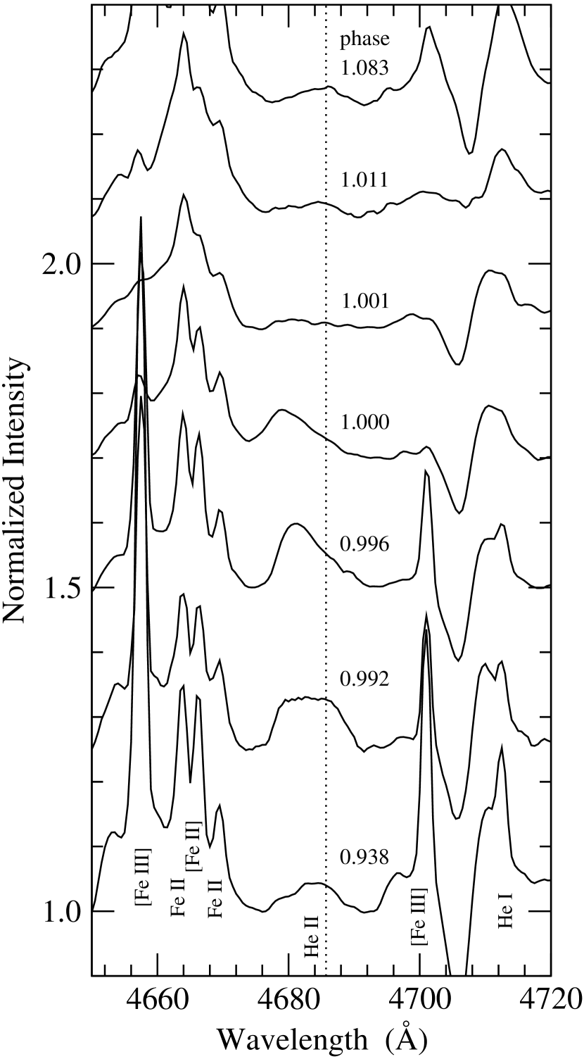
Figure 1: Sample of He II $\lambda$4686 Å line profiles labeled by phase of the 2022.1–d period. The vertical dotted line indicates the rest wavelength of He II $\lambda$4686 Å.

Data reduction was done with IRAF package in the standard way. The spectral resolution was degraded to 0.5Å/pixel in order to enhance the signal–to–noise ratio. Most of the spectra used here have S/N$>$100 in the stellar continuum and some of them twice as much, specially around ph$=$0.2–0.8, when many spectra were co–added. We detected an emission line at $\sim$4680–85 Å (Figure 1), that we suggest to be He II $\lambda$4686 Å. We searched for possible transitions in the range 4670–4700 Å and found none from species that are typical of the $\eta$ Carinae spectrum. He II $\lambda$4686 Å has never been detected with certainty before, as discussed by Hillier and Allen (1992 and references therein), who reported an upper limit of 1Å. The line showed up in almost all of our high quality spectra, except in a few ones of lower S/N. Paradoxically, this line is faint in high excitation phases and strong during the event, contrarily to the behavior of the high excitation forbidden lines. In Figure 1 we display a sample of spectra collected in 2003, ordered by phase of the 2022.1–d period.

In order to evaluate the errors, we measured several times each line, with different assumptions for the continuum. The errors were 20–100 mÅ in the equivalent widths (EWs) and 10–110 Km s^-1 in the radial velocities (RVs) of the line centroid (V_cen) and are displayed in Figures 2 and 3. Those are formal errors; systematic errors may also be present, for example introduced by the rectification of the continuum. The fit to the continuum was done by a 3rd order polynomial, what introduces only low frequencies and has little influence on scales comparable to the extent of a spectral line. Structures in the flatfielding image could introduce distortions in the continuum, although of low frequency, since we used always the same observational setup and data reduction procedures. The EWs are affected by an additional type of systematic error: line blending, that prevents the assessment of the local continuum and consequently the extension of the line wings. This makes the measurements of EWs and FWHM ($\sim$500–600 Km s^-1) somewhat underestimated, as is the case for almost all other spectral lines in the rich spectrum of $\eta$ Car. The position of the line centroid is much more robust and is affected only by the S/N ratio, consequently the errors can be better judged from the overall scatter in the RV curve.

The slit width was kept fixed at $\sim$1.5”, and this seems relevant, since a fraction of the He II emission appears to be extended. Our data of 1997 and 2002, when compared with contemporaneous spectra taken with FEROS spectrograph at ESO ($\sim$3.6” fiber entrance), result in smaller EWs. The comparison of our 2003 data with those taken with STIS on board of HST ($\approx$0.1” slit width) result in larger EWs, indicating that the EWs are larger for wider slits. This is the opposite of that reported by Hillier and Allen (1992) for H I, He I and Fe II lines in the Homunculus, which are smaller than those in the central object. He II seems to be intrinsically in emission near the central source, since dust scattering would preserve the equivalent widths. The line shape and radial velocity are unchanged with the slit aperture, indicating that most of the emission should arise from the central object. In fact, long–slit CCD HST/STIS spectra (52”x 0.1”) collected prior to the 2003.5 event (T.R. Gull, private communication) show that the He II emission was confined to 0.1” (2–pixel limit) in the East–West direction. However, the emission could be extended in other directions outside the slit. Although this question is relevant, the data available to us are insufficient to derive any firm conclusion and we will restrict our analysis to the homogeneous Brazilian set of data.

In Figure 2 we see that the strength of the He II line is very weak along the 5.5–yr cycle at the level of EW$\approx$100 mÅ. It starts strengthening around ph$\approx$0.8, jumps to EW$=$873 mÅ just before ph$=$1.0, and after a brief fading, it rises again, reaching a local maximum (EW$=$300 mÅ) at ph$\approx$1.04. In Figure 3a we display a zoom in the EW curve around ph$=$1.0, showing a peak centered at ph$=$0.994, a fast drop after ph$=$1.0 and a minimum around ph$=$1.003. In Figure 3b we show the RV curve as measured from the velocity of the line centroid. The velocity becomes more and more negative as the system approaches ph$=$1.0, reaching a sharp minimum (V_cen=$-$396 Km s^-1) at ph$=$1.001. After ph$=$1.002, uncertainties in RVs increase significantly and we will not comment them any further.

3 Interpretation and Discussion

The interpretation of the intensity curve of He II $\lambda$4686 Å as well as of its radial velocity may provide important insights about the nature and structure of the system. The first thing to notice is the strong similarity between the He II emission curve and the X–ray light curve (Corcoran et al., 2001; Ishibashi et al., 1999). Both emissions start to enhance at ph$=$0.8, peak just before ph$=$1.0, drop to near zero intensity at about ph$=$1.001 and return to normal intensity after ph$\sim$1.1. A noticeable difference between the two light curves is that He II has a much narrower and prominent peak (centered at ph$=$0.994) than the X–ray light curve, which has its maximum at ph$=$0.985. The X–ray emission is thought to be originated from the shock wave of the colliding winds in a binary system. Its ”eclipse” has been modeled by PC, who derived system parameters that will be adopted as a reference frame in the following discussion. Given this similarity, it is tempting to interpret the He II emission as being originated from photoionization by X–ray or by the ultraviolet (UV) photons associated to this source.

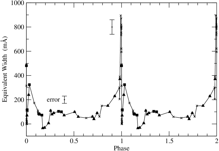
Figure 2: He II $\lambda$4686 Å line EW curve for the last three cycles - $\blacktriangle$s are for 1997/98; $\blacksquare$s for 1992; and xs for 2003.

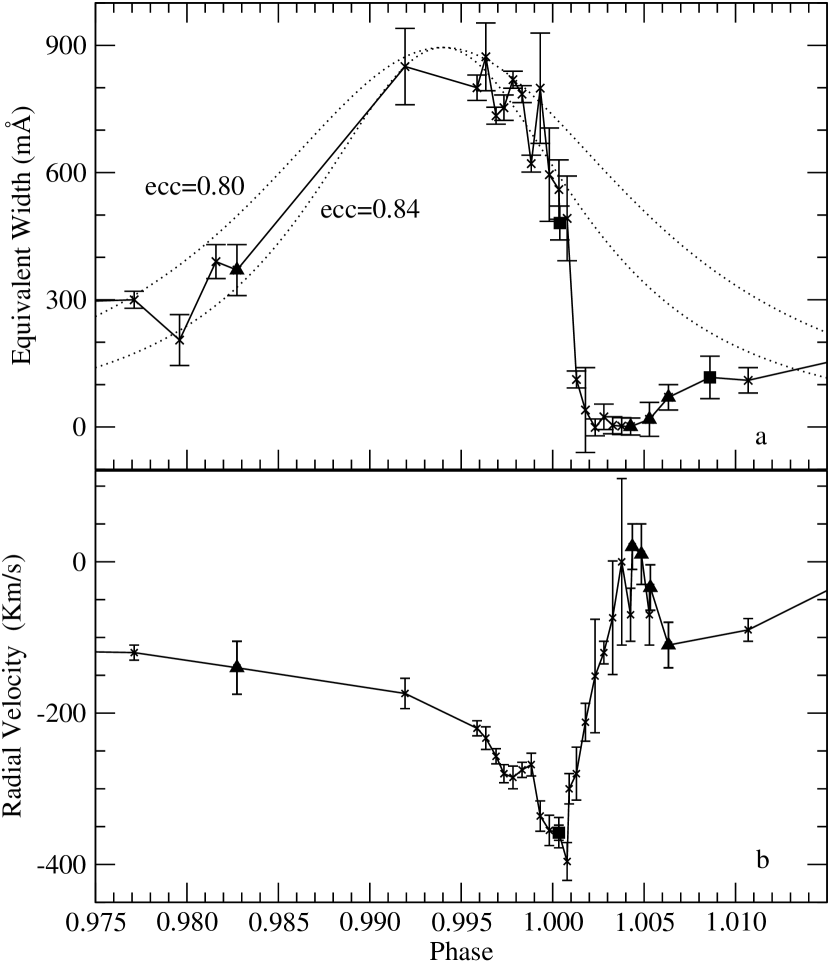
Figure 3: Zoom in He II $\lambda$4686 Å variations around ph$=$0. Upper panel: solid line EW curve; dotted lines He II emission models. Lower panel: RV curve. Same symbols as in Figure 2

.

Near periastron, the X–ray and UV ionizing photons are mostly unobserved as they are absorbed by the intervening gas along the line of sight. However, gas near the shock wave (including the winds of the primary and of the secondary stars) may still be directly exposed to this ionization. The He II $\lambda$4686 Å, at its maximum intensity, has a luminosity of $L_{HeII}$$\sim$100 L_⊙ (assuming the somewhat uncertain values of V$\sim$7.5 and Av$\sim$6 for the central source). This amounts to about 9$\times$10⁴⁶ photons per second. In order to produce this emission, a luminous source of ionizing soft X–ray and ultraviolet photons is required; the peak luminosity of the unabsorbed X–rays in the range 2–10 kev is only L_Xunabs$=$67 L_⊙ Ishibashi et al. (1999). Detailed hydrodynamical numerical calculations by PC show that when the velocity of the secondary’s wind is large (V₂$\sim$3000 Km s^-1) the energy spectrum behaves like a power law, at soft X–rays. From their Figure 3 we derive a spectrum of L_ϵ$=$2.5$\times$10${}^{35}\epsilon$^-2.7 ergs s^-1 kev^-1 for the system parameters favored by those authors ($\dot{M}_{2}$$=$10^-5 M_⊙ yr^-1 and V₂$=$3000 Km s^-1). In the case that this spectrum can be extrapolated down to 54 eV (He⁺ threshold ionization), the total luminosity would be L_ion$=$5200 L_⊙. This extrapolation seems to be reasonable since the energy loss by the wind from the secondary star alone is $\dot{E}$₂$=$7500 L_⊙. The total number of photons emitted by this source is N_ion$=$2.5$\times$10⁴⁷ ph s^-1 what amounts to $\approx$3 times the observed number of He II $\lambda$4686 Å photons. If we add to this the energy from the shock of the primary star, this number will be even larger. We conclude that near periastron the production of ionizing photons is of the right order of magnitude to produce the observed He II emission via photoioniozation. It is worth noting that only $\approx$1% of the kinetic energy from the wind of the secondary star is radiated in the 2–10 kev band. Where are the other 99% going to? The detection of He II emission may be the first hint that they are mostly radiated in the UV.

The fact that the bulk of the He II emission is short lived in terms of the EW curve (lasting for $\approx$1% of the orbital cycle) suggests that its peak indicates the passage of the periastron – and this is quite interesting. This timing is not precisely determined either by the X–ray light curve (as the wind of the primary star is optically thick to X–ray absorption) or by the high excitation emission lines (that are emitted far away), although the low ionization event is generally believed to be associated to the periastron approach. The timing of the periastron (ph$=$0.994) would be the second orbital parameter determined with accuracy, besides the period.

A solution to the X–ray light curve was obtained by PC in which the wind–wind shock before eclipse is observed through the opening angle in such a way that the X–ray source is seen through the non-absorbing wind from the secondary star. After the shock front passes through the line of sight, the X–rays are absorbed by the wind from the primary star. In this way the symmetry of the observed emission is broken and one gets a post–minimum flux that is lower then the pre–minimum one. If we assume that the periastron passage occurs at ph$=$0.994, we are able to fit the X–ray light curve with the parameters ecc$=$0.84 and the longitude of the periastron of the primary star, $\omega$$=$212^o. These parameters predict a superior conjunction for the secondary star with a true anomaly of $\theta$$=$58^o at the phase where our observations show a sharp drop in EWs and a gradient reversal in the RV curve. Does this suggest an eclipse? This question brings us to another one: where is the region of He II emission located?

The large values of the velocity cannot be associated to the shock wave itself as the gas in that region has nearly the velocity of the center of mass. A similar argument could be made with respect to the wind of the primary star. The terminal velocity of the primary star is about $\sim$500 Km s^-1; at the phase under consideration, the shock wave is quite near the primary and the velocity of the wind is still far from terminal. In addition, the shock wave is symmetric with respect to the orbital plane and the line of sight imposes a projection of i$\sim$45^o. In this scenario, it seems difficult to combine the emission and radial velocity behavior as displayed in Figure 3. In particular, the radial velocity is bluest when the emission has dropped to its half maximum intensity, after reaching the peak. If we suppose that the emission comes from the near side of the primary star, ionized to He⁺⁺ by the secondary or by the shock, one would expect maximum blue-shift at maximum emission.

Perhaps a more promising explanation is that the He II emission comes from the wind of the secondary star, ionized by the external UV emission from the shock wave. This would produce an ionization front that divides this wind into a zone of He⁺ and a zone of He⁺⁺. The He⁺⁺ zone would be directly exposed to the UV emission and an asymmetric configuration is produced with respect to the secondary star. This asymmetry will cause a blue-shifted emission when the system is seen at an appropriate angle. As periastron occurs at ph$=$0.994 and the longitude of periastron is $\omega$$=$212^o, the ionized He II emitting wind from the secondary star should naturally display negative velocities when seen from the line of sight of the observer. The terminal velocity of the wind from the secondary star is about $\sim$3000 Km s^-1 (PC), so one might expect higher velocities and line widths than observed. However, the emission is likely to come from deep into the wind where the density is higher and the velocity smaller, still far from the terminal velocity. In addition, the inclination of the system is about i$\approx$45^o, which reduces the velocity by about $\sim$cosi. Let us assume a highly idealized model of an ionized hemisphere with concentric layers of radii r and normal velocity law: v$=$v₀(1-R₂/r)^β (where R₂ is the radius of the secondary star). As the emissivity is proportional to the square of the density, the contribution of each layer to the line intensity is proportional to $\sim$r^-2. The peak of the line profile should, therefore, be emitted at velocities that correspond to the innermost ionized zone. We estimate that in order to produce the observed RVs (–400 Km s^-1), the innermost ionized zone should occur at r$\approx$ 4 R₂, for $\beta$$=$1. At periastron, the distance from the secondary star to the innermost zone is 60 R_⊙, to the stagnation shock front is 210 R_⊙ and to the surface of the primary, 360 R_⊙.

The observed line widths (FWHM$\sim$500–600 Km s^-1) require a radius that is somewhat smaller. However, as pointed out before, the observed FWHM is a lower limit because the line wings/continuum are difficult to be determined with accuracy. If the He II emitting wind is indeed eclipsed, one would expect that when the intensity is at its half maximum, half of the wind should be eclipsed and the velocity should be most negative; this is so because, given the structure of the shock wave and its skew angle (see PC), at this time the portion of the wind with more positive velocity is already eclipsed. This prediction is confirmed as both events occur at the same phase (ph$=$1.001).

The sharpness of the fading phase of the He II intensity curve (Figure 3a) is a challenging characteristic that demands restrictive parameters to be modeled. For example, if it is due to an eclipse, to be caused by the primary star or by its wind, this wind cannot be isotropic with a mass loss rate of $\dot{M}_{1}$$=$2.5$\times$10^-4 M_⊙ yr^-1 (PC); this would be optically thick for electron scattering at too large a radius. As an alternative, one could suppose that the Homunculus configuration, with a bipolar and equatorial disk could be scaled down to the size of the binary system. In this situation, the polar wind would be responsible (partially of totally) for the eclipse of the He II emission and the equatorial disk, for the X–ray emitting shock wave. Such a configuration has also been proposed on the basis of other observational (Smith et al., 2003; van Boekel et al., 2003) and theoretical (Maeder & Desjacques, 2001) considerations. However, results from spectral modeling in the optical (Hillier et al., 2001) and infrared interferometry (van Boekel et al., 2003) have found mass-loss rates of $\dot{M}_{1}$$\sim$10^-3 M_⊙ yr^-1. Such determinations are clearly in contradiction with our eclipse hypothesis, unless the mass-loss rate is highly anisotropic.

In the wind–wind collision model, the X–ray luminosity is inversely proportional to the separation of the stars, $L_{X}~{}\alpha~{}D^{-1}$, so that at periastron, X–ray luminosity is maximum (Usov, 1992). At the same time, the angle subtended by the secondary star as seen from each point of the shock wave is $\alpha~{}D^{-1}$, making the fraction of the UV and X–ray photons that are absorbed by the wind from the secondary star to go with the square of the inverse of the distance between the two stars. Therefore one expects that the luminosity of the He II line to be inversely proportional to the cube of the stellar separation: $L_{HeII}~{}\alpha~{}D^{-3}$. Figure 3 shows that the rising phase and the peak of the He II EW curve can be well described by a function of the form $L_{HeII}~{}\alpha~{}D^{-3}$ for ecc$=$0.82–0.84. This agreement, however, does not prove that the He II emission comes from the wind of the secondary star; any model that provides a dependence as the inverse of the cube of the distance would be as good as well.

In this simplified model we suppose that the emission is highly concentrated. We should keep in mind that there are indications for extended emission as well, so that the real picture is actually more complicated, but its detailed analysis and modeling are beyond the scope of this Letter.

References

- Corcoran et al. (2001) Corcoran, M.F., Ishibashi, K., Swank, J.H., & Petre 2001 ApJ, 547,1034
- Corcoran et al. (2004) Corcoran, M.F. et al. 2004, in preparation
- Damineli (1996) Damineli, A. 1996, ApJ, 460, L49
- Damineli, Conti & Lopes (1997) Damineli, A., Conti, P.S., & Lopes, D.F. 1997, New Astr., 2, 107 (DCL)
- Davidson (1997) Davidson, K. 1997, New Astr., 2, 387
- Feast et al. (2001) Feast, M., Whitelock, P., & Marang, F. 2001, MNRAS, 322, 741
- Hillier et al. (2001) Hillier, D.J., Davidson, K., Ishibashi, K., Gull, T. 2001, ApJ, 553, 837
- Hillier and Allen (1992) Hillier, J.D. & Allen, D.A. 1992, A&A, 262, 153
- Ishibashi et al. (1999) Ishibashi, K., Corcoran, M.F., Davidson, K., et al. 1999, ApJ, 524, 983
- Maeder & Desjacques (2001) Maeder, A. & Desjacques, V., 2001, A&A 372, L9
- Pittard & Corcoran (2002) Pittard, J.M., & Corcoran, M.F. 2002, A&A 383, 636 (PC)
- Smith et al. (2003) Smith, N., Gull, T.R., Ishibashi, K., & Hillier, J. 2003, ApJ, 586, 432
- Usov (1992) Usov, V.V. 1992, ApJ, 389, 635
- van Boekel et al. (2003) van Boekel, R., Kervella, P., Scholler,M. et al. 2003, A&A, 401, L37
- van Genderen et al. (2003) van Genderen, A., Sterken, C., Allen, W.H., & Liller, W. 2003, A&A 412, L25
- Whitelock et al. (2004) Whitelock, P., Feast, M.W. , Marang, F., & Breedt, E. 2004, MNRAS, 352, 1365