Nuclear Reaction Network for Primordial Nucleosynthesis: a detailed analysis of rates, uncertainties and light nuclei yields.

Abstract

We analyze in details the standard Primordial Nucleosynthesis scenario. In particular we discuss the key theoretical issues which are involved in a detailed prediction of light nuclide abundances, as the weak reaction rates, neutrino decoupling and nuclear rate modeling. We also perform a new analysis of available data on the main nuclear processes entering the nucleosynthesis reaction network, with particular stress on their uncertainties as well as on their role in determining the corresponding uncertainties on light nuclide theoretical estimates. The current status of theoretical versus experimental results for ²H, ³He, ⁴He and ⁷Li is then discussed using the determination of the baryon density as obtained from Cosmic Microwave Background anisotropies.

1 Introduction

The huge amount of data coming from astronomical observations in the recent years represents the basic impulse and the a priori condition for the development of what has been fairly called precision cosmology. Results on Cosmic Microwave Background (CMB) anisotropies by the WMAP Collaboration [1] and the second data release of the Sloan Digital Sky Survey [2] are perhaps the most striking examples of such a massive effort. On one hand these experimental results give a beautiful confirmation of our present understanding of the evolution of the Universe and provide accurate information on several cosmological parameters. On the other hand they stimulated further efforts in increasing the level of accuracy of theoretical studies. This general trend is clearly recognized in the analysis of several cosmological observables, such as the CMB anisotropies and polarization, the Large Scale Structure formation and, for what matters for the present study, Big Bang Nucleosynthesis.

Big Bang Nucleosynthesis (BBN) is one of the pillars of the cosmological model, and it also represents one of the most powerful tools to test fundamental physics. Presently, this aspect is even more relevant than in the past. In fact since the baryon density is now independently measured with very high precision by CMB anisotropies, the theory of BBN is basically parameter free in its standard formulation so that comparing experimental determination of light nuclides with corresponding theoretical estimate can severely constraint any exotic physics (for a general overview on the subject, see the review by B.D. Fields and S. Sarkar in the Particle Data Book [3] and references therein).

In the last decade the accuracy of BBN theory has been increased by a careful analysis of many of its key aspects. The accuracy of the weak reactions which enter the neutron/proton chemical equilibrium has been pushed up to less than percent level [4, 5]. Similarly, the neutrino decoupling has been carefully studied by several authors by explicitly solving the corresponding kinetic equations, see e.g. [6, 7] and References therein. These two issues are mainly affecting the prediction of ⁴He mass fraction, which presently has a very small uncertainty, of the order of 0.1 %, due to the experimental uncertainty on neutron lifetime.

One of the most relevant aspects to get an accurate determination of light nuclide abundances is the evaluation of the several nuclear reaction rates which enter the BBN reaction network, as well as the corresponding uncertainties. This task involves a careful study of the available data or predictions on each reaction, the choice of a reasonable protocol to combine them in order to obtain a best estimate and an error and finally, the calculation of the corresponding thermal rates entering the BBN network.

After the first analysis performed in [8]-[12], and later studies [13, 14], which have been the status of the art results for decades, an important step has been the publication of a large nuclear rate catalogue by NACRE Collaboration [15]. Despite of the fact that this catalogue by its own nature is an all-purpose compilation and not only devoted to BBN studies, and that in particular not all BBN reactions are in fact covered, nevertheless it is an extremely important reference. Other nuclear databases, such as [16] or [17] collect relevant information on cross sections, nuclear parameters and beta-unstable nuclide lifetimes.

Recently, new and more precise experimental data have been obtained for relevant nuclear reactions in the energy range of interest for the BBN, as for example the LUNA Collaboration results on ²H + p $\leftrightarrow$ $\gamma$ + ³He process [18]. In view of this new developments and of the fact that as stressed already there is presently a demand for an increased precision of BBN predictions, it is important to undertake a critical review of the whole BBN nuclear network, and in particular to quantify the uncertainties which affect the nuclide abundances as obtained by propagating the error on the several nuclear rates entering this network. This study is the main goal of this paper. Similar analysis has been also performed in [19], [20] and [21].

In the following Sections we cover all the main theoretical aspects of BBN with the aim of providing a self contained description of the several issues which enter an accurate determination of nuclide abundances. To help the reader to distinguish the review parts collecting the results of previous studies from the ones devoted to original new results first presented in the present paper, the former have been tagged by a “$*$”.

In Section 2 we review in details the general BBN framework by recalling the corresponding set of equations. We also describe the neutrino decoupling as obtained via a numerical solution of the corresponding kinetic equation, including as in [7] the effect of QED radiative corrections and in particular the non thermal distortion in neutrino distribution functions due to $e^{+}-e^{-}$ entropy release.

Section 3 is devoted to the analysis of all main rates entering the BBN network. We first review the calculation of $n\leftrightarrow p$ weak rates, evaluated up to order $\alpha$ QED radiative corrections, and also taking into account the effect of finite nucleon mass and thermal radiative effects. We also discuss the effect on these rates of neutrino decoupling. After introducing the nuclear astrophysics formalism used in our analysis, we describe our method for the data reduction and rate estimate and finally describe in details the data and the results obtained for all leading reactions entering the BBN network. We also analyze some sub-leading reaction which, in view of the present uncertainties on the corresponding rates, may still play a role in determining the eventual light nuclide yields.

In Section 4 we first summarize the present status of observations on ²H, ⁴He, and ⁷Li, as well as what is known on other light nuclides, such as ³He or ⁶Li. We then give our results for main nuclide abundances, as obtained by a FORTRAN code that we have developed in the recent years modifying the original public code of [22] in order to consistently introduce all the issues described in this paper (neutrino decoupling, radiative corrections to $n\leftrightarrow p$ rates, etc.) and employing a different numerical resolution method, as explained in Section 2.3.

All results are given for a standard BBN scenario, with three non degenerate neutrinos, and the baryon density as fixed by the WMAP result combined with results of CBI and ACBAR experiments on CMB anisotropies, as well as with 2dFGRS data on power spectrum, $\omega_{b}\equiv\Omega_{b}h^{2}=0.023{\pm}0.001$ [1], where $\Omega_{b}$ is the ratio of the baryonic matter density with respect to the critical one, and $h$ is the Hubble constant in units of 100 Km $s^{-1}$ Mpc^-1. A careful study of this case seems to us of particular relevance since there are no free parameters left. Comparing experimental results with theoretical expectations is therefore a clean consistency test of the simplest BBN dynamics. It may also give useful hints to point out possible systematics in the experimental results for nuclide abundances. A particular stress is given to the present theoretical uncertainty on each nuclide yield, as well as on the role of the several nuclear rates in building up this uncertainty. We also comment on the impact of different values adopted for $\omega_{b}$ as obtained by WMAP with different choices of priors or combining different observations. Finally, we discuss how the baryon density is constrained by BBN as compared to the very precise measurement by CMB anisotropies.

Our Conclusions are reported in Section 5.

2 The BBN general framework $*$

2.1 Generalities $*$

We consider $N_{nuc}$ species of nuclides, whose number densities, $n_{i}$, are normalized with respect to the total number density of baryons, $n_{B}$,

$$X_{i}=\frac{n_{i}}{n_{B}}\quad\quad\quad i=n,\,p,\,^{2}{\rm H}...~{}~{}~{}.$$ (2.1)

A list of all nuclides which are typically included in a BBN analysis is reported in Table 1. To quantify ²H, ⁴He and ⁷Li abundances, we also use in the following the parameters

$$X_{{}^{2}{\rm H}}/X_{p},\,\,\,\,\,X_{{}^{3}{\rm He}}/X_{p},\,\,\,\,\,Y_{p}=4X_{{}^{4}{\rm He}},\,\,\,\,\,X_{{}^{7}{\rm Li}}/X_{p}~{}~{}~{},$$ (2.2)

i.e. the ²H, ³He and ⁷Li number density normalized to hydrogen, and the ⁴He mass fraction. For the sake of clarity we stress that our notation $X_{i}$ for the nuclide number density normalized to hydrogen is not adopted by all authors. The symbols $Y_{i}$ can be also frequently found in the literature.

1)	n	7)	6Li	13)	10B	19)	13C	25)	15O
2)	p	8)	7Li	14)	11B	20)	13N	26)	16O
3)	2H	9)	7Be	15)	11C	21)	14C
4)	3H	10)	8Li	16)	12B	22)	14N
5)	3He	11)	8B	17)	12C	23)	14O
6)	4He	12)	9Be	18)	12N	24)	15N

Table 1: Nuclides considered in the BBN analysis

The neutrino/antineutrino distributions are denoted by $f_{\nu_{e}}(\left|\vec{p}\right|,t)$, $f_{\bar{\nu}_{e}}(\left|\vec{p}\right|,t)$ and

$$f_{\nu_{\mu}}=f_{\nu_{\tau}}\equiv f_{\nu_{x}}(\left|\vec{p}\right|,t)~{}~{}~{},~{}~{}~{}f_{{\bar{\nu}}_{\mu}}=f_{{\bar{\nu}}_{\tau}}\equiv f_{{\bar{\nu}}_{x}}(\left|\vec{p}\right|,t)~{}~{}~{},$$ (2.3)

In the temperature range we are interested in, $10\,{\rm MeV}>T>0.01\,{\rm MeV}$, electrons and positrons are kept in thermodynamical equilibrium with photons by fast electromagnetic interactions. Thus, they are distributed according to a Fermi-Dirac function $f_{e^{\pm}}$, with chemical potential $\mu_{e}$.

The set of differential equations ruling primordial nucleosynthesis is the following (see for example [23, 24, 25])

$$\frac{\dot{R}}{R}=H=\sqrt{\frac{8\,\pi G_{N}}{3}~{}\rho}~{}~{}~{},$$ (2.4)

$$\frac{\dot{n}_{B}}{n_{B}}=-\,3\,H~{}~{}~{},$$ (2.5)

$$\dot{\rho}=-\,3\,H~{}(\rho+{\rm p})~{}~{}~{},$$ (2.6)

$$\dot{X}_{i}=\sum_{j,k,l}\,N_{i}\left(\Gamma_{kl\rightarrow ij}\,\frac{X_{l}^{N_{l}}\,X_{k}^{N_{k}}}{N_{l}!\,N_{k}!}\;-\;\Gamma_{ij\rightarrow kl}\,\frac{X_{i}^{N_{i}}\,X_{j}^{N_{j}}}{N_{i}!\,N_{j}!}\right)\equiv\Gamma_{i}(X_{j})~{}~{}~{},$$ (2.7)

$$L\left(\frac{m_{e}}{T},{\phi_{e}}\right)=\frac{n_{B}}{T^{3}}~{}\sum_{j}Z_{j}\,X_{j}~{}~{}~{},$$ (2.8)

$$\left(\frac{\partial}{\partial t}-H\,\left|\vec{p}\right|\frac{\partial}{\partial\left|\vec{p}\right|}\right)\,f_{\nu_{\alpha}}(\left|\vec{p}\right|,t)=I_{\nu_{\alpha}}\left[f_{\nu_{e}},f_{\bar{\nu}_{e}},f_{\nu_{x}},f_{\bar{\nu}_{x}},f_{e^{-}},f_{e^{+}}\right]~{}~{}~{},$$ (2.9)

with $\nu_{\alpha}=\nu_{e}$, $\bar{\nu}_{e}$, $\nu_{x}$, $\bar{\nu}_{x}$, where $\rho$ and ${\rm p}$ denote the total energy density and pressure, respectively,

$$\rho = \rho_{\gamma}+\rho_{e}+\rho_{\nu}+\rho_{B}=\rho_{NB}+\rho_{B}~{}~{}~{},$$ (2.10)

$${\rm p} = {\rm p}_{\gamma}+{\rm p}_{e}+{\rm p}_{\nu}+{\rm p}_{B}={\rm p}_{NB}+{\rm p}_{B}~{}~{}~{},$$ (2.11)

where $i,j,k,l$ denote nuclides, $\rho_{B}$ and $\rho_{NB}$ are the baryon and non baryonic energy density respectively, $Z_{i}$ is the charge number of the $i-$th nuclide, and the function $L(\xi,y)$ is defined as

$$L(\xi,\omega)\equiv\frac{1}{\pi^{2}}\int_{\xi}^{\infty}d\zeta~{}\zeta\,\sqrt{\zeta^{2}-\xi^{2}}~{}\left(\frac{1}{e^{\zeta-\omega}+1}-\frac{1}{e^{\zeta+\omega}+1}\right)~{}~{}~{}.$$ (2.12)

Equation (2.4) is the definition of the Hubble parameter, $H$, with $G_{N}$ the gravitational constant, whereas Equations (2.5) and (2.6) state the total baryon number and entropy conservation in the comoving volume, respectively. The set of $N_{nuc}$ Boltzmann equations (2.7) describes the density evolution of each nuclide specie, with $\Gamma_{kl\rightarrow ij}$ the rate per incoming particles averaged over kinetic equilibrium distribution functions. While in fact chemical equilibrium among nuclides cannot be assumed, as BBN strongly violates Nuclear Statistical Equilibrium, it is perfectly justified to assume kinetic equilibrium, which is maintained by fast strong and electromagnetic processes. Equation (2.8) states the Universe charge neutrality in terms of the electron chemical potential, with $\phi_{e}\equiv\mu_{e}/T$ and $T$ the temperature of $e^{\pm},\gamma$ plasma, and finally Equations (2.9) are the Boltzmann equations for neutrino species, with $I_{\nu_{\alpha}}\left[f_{\nu_{e}},f_{\nu_{x}}\right]$ standing for the collisional integral which contains all microscopic processes creating or destroying the specie $\nu_{\alpha}$. In the following we do not consider neutrino oscillations, whose effect has been proved to be sub-leading and affect ${}^{4}{\rm He}$ mass fraction for $\sim 1{\cdot}10^{-4}$ [26].

In the standard scenario of no extra relativistic degrees of freedom at BBN epoch apart from photons and neutrinos, the neutrino chemical potential is bound to be a small fraction of neutrino temperature, smaller than approximately $|\xi_{\nu}|\equiv|\mu_{\nu}/T_{\nu}|\leq 0.1$ [20, 27, 28, 29]. This bound applies to all neutrino flavors, whose distribution functions are homogenized via flavor oscillations [27, 30]. In view of this, as far as this analysis is concerned, we will focus on non degenerate neutrinos, so that $f_{\nu_{e}}=f_{\bar{\nu}_{e}}$ and $f_{\nu_{x}}=f_{\bar{\nu}_{x}}$.

The neutrino energy density and pressure are defined in terms of their distributions as

$$\rho_{\nu}=3\,{\rm p}_{\nu}=2\,\int\frac{d^{3}p}{(2\pi)^{3}}\,\left|\vec{p}\right|\,\left[f_{\nu_{e}}+2\,f_{\nu_{x}}\right]~{}~{}~{},$$ (2.13)

whereas for baryons we have

$$\rho_{B} = \left[M_{u}+\sum_{i}\left(\Delta M_{i}+\frac{3}{2}\,T\right)~{}X_{i}\right]n_{B}\,\,\,,$$

$${\rm p}_{B} = T\,n_{B}\,\sum_{i}X_{i}\,\,\,.$$ (2.14)

with the $\Delta M_{i}$ and $M_{u}$ the i-th nuclide mass excess and the atomic mass unit respectively. Finally, pressure and energy density for the electromagnetic plasma ($e^{\pm}$ and $\gamma$) is calculated by improving the incoherent scattering limit result (particles correspond to poles of the propagators at, respectively, $p^{2}=0$ (photons) and $p^{2}=m_{e}^{2}$ (electrons/positrons)) and considering the effect of finite temperature QED corrections. It has been shown in fact that at the time of BBN, these corrections affect Equations (2.4)-(2.9) at some extent and slightly influence the ⁴He abundance [4]. Indeed finite temperature QED corrections modify the electromagnetic plasma equation of state and thus influence Equation (2.6), the expression of the expansion rate $H$ and, as it will be discussed in the following, the conversion rates $n\leftrightarrow p$.

The change in the electromagnetic plasma equation of state can be evaluated by considering the corrections induced on the $e^{\pm}$ and photon masses, using the tools of Real Time Finite Temperature Field Theory [31]. For the electron/positron mass, up to order $\alpha\equiv e^{2}/\left(4\,\pi\right)$, we find the additional finite temperature contribution [7, 32]

$$\delta m_{e}^{2}\left(|\mathbf{p}|,\,T\right) = \frac{2\,\pi\,\alpha\,T^{2}}{3}+\frac{4\,\alpha}{\pi}\,\int_{0}^{\infty}d|\mathbf{k}|\,\frac{|\mathbf{k}|^{2}}{E_{k}}\,\frac{1}{{\rm e}^{E_{k}/T}+1}$$ (2.15)

$$- \frac{2\,m_{e}^{2}\,\alpha}{\pi\,|\mathbf{p}|}\,\int_{0}^{\infty}d|\mathbf{k}|\,\frac{|\mathbf{k}|}{E_{k}}\,\log\left|\frac{|\mathbf{p}|+|\mathbf{k}|}{|\mathbf{p}|-|\mathbf{k}|}\right|\frac{1}{{\rm e}^{E_{k}/T}+1}~{}~{}~{},$$

where $E_{k}\equiv\sqrt{|\mathbf{k}|^{2}+m_{e}^{2}}$. We note that in this equation the term depending on the $e^{\pm}$ momentum $|\mathbf{p}|$ contributes for less than $10\,\%$ to $\delta m_{e}^{2}\,$ and thus it can be safely neglected. This highly simplifies the analysis and is fully legitimate at the level of precision we are interested in (corrections to $Y_{p}$ at the level of $0.0001$).

The renormalized photon mass in the electromagnetic plasma is instead, up to order $\alpha$, given by (see for example [33])

$$\delta m_{\gamma}^{2}\left(T\right)=\frac{8\,\alpha}{\pi}\,\int_{0}^{\infty}d|\mathbf{k}|\,\frac{|\mathbf{k}|^{2}}{E_{k}}\,\frac{1}{{\rm e}^{E_{k}/T}+1}~{}~{}~{}.$$ (2.16)

The corrections (2.15) and (2.16) modify the corresponding dispersion relations as $E_{i}^{2}=|\mathbf{k}|^{2}+m_{i}^{2}+\delta m_{i}^{2}\left(T\right)\,$ ($i=e,\,\gamma$). Thus the total pressure and energy density of the electromagnetic plasma result to be

$${\rm p}_{\gamma}+{\rm p}_{e} = \frac{T}{\pi^{2}}\,\int_{0}^{\infty}d|\mathbf{k}|\,|\mathbf{k}|^{2}\,\,\log\left[\frac{\left(1+{\rm e}^{-E_{e}/T}\right)^{2}}{\left(1-{\rm e}^{-E_{\gamma}/T}\right)}\right]~{}~{}~{},$$ (2.17)

$$\rho_{\gamma}+\rho_{e} = \left(T\,\frac{d}{dT}-1\right)({\rm p}_{\gamma}+{\rm p}_{e})~{}~{}~{}.$$ (2.18)

Expanding these expressions with respect to $\delta m_{e}^{2}$ and $\delta m_{\gamma}^{2}$, one obtains the first order correction

$$\delta{\rm p}_{\gamma}+\delta{\rm p}_{e} = -\int_{0}^{\infty}\frac{|\mathbf{k}|\,d|\mathbf{k}|}{2\,\pi^{2}}\left[\frac{|\mathbf{k}|}{E_{k}}\,\frac{\delta m_{e}^{2}\left(T\right)}{{\rm e}^{E_{k}/T}+1}+\frac{1}{2}\,\frac{\delta m_{\gamma}^{2}\left(T\right)}{{\rm e}^{k/T}-1}\right]\,\,.$$ (2.19)

The energy density is then obtained by using the expression for ${\rm p}_{\gamma}+{\rm p}_{e}$ in Equation (2.18).

The equations (2.4), (2.6) and (2.9) can be solved separately since they are essentially determined by relativistic particles, and only negligibly affected by the baryons contribution. This allows to solve the evolution of the neutrino species first, and then to substitute the result into the remaining equations.

2.2 Neutrino decoupling $*$

The evolution of neutrino distribution function can be highly simplified by using the scale factor as evolution variable $x\equiv m_{e}\,a$, and the comoving momentum $y\equiv\left|\vec{p}\right|\,a$. We also define the rescaled photon temperature as $\bar{z}\equiv T\,a$. By using these definitions, the set of equations (2.6) and (2.9), once baryonic contribution is neglected, becomes

$$\frac{d}{dx}\bar{\rho}(x)=\frac{1}{x}\,\left(\bar{\rho}-3\bar{{\rm p}}\right)~{}~{}~{},$$ (2.20)

$$\frac{d}{dx}\,f_{\nu_{\alpha}}(x,y)=\frac{1}{xH}\,I_{\nu_{\alpha}}\left[f_{\nu_{e}},f_{\nu_{x}}\right]~{}~{}~{},~{}~{}~{}~{}\mbox{with}~{}~{}~{}\nu_{\alpha}=\nu_{e},\nu_{x}~{}~{}~{}.$$ (2.21)

In Equation (2.20), which states the conservation of the total energy momentum, $\bar{\rho}$ and $\bar{{\rm p}}$ are the dimensionless energy density and pressure of the primordial plasma, respectively,

$$\bar{\rho}=\rho\left(\frac{x}{m_{e}}\right)^{4}\sim\rho_{NB}\left(\frac{x}{m_{e}}\right)^{4},\,\,\qquad\bar{{\rm p}}={\rm p}\left(\frac{x}{m_{e}}\right)^{4}\sim{\rm p}_{NB}\left(\frac{x}{m_{e}}\right)^{4}~{}~{}~{}.$$ (2.22)

As in Reference [7, 34] the unknown neutrino distributions are parameterized as

$$f_{\nu_{\alpha}}\left(x,y\right)=\frac{1}{e^{y}+1}\left(1+\delta f_{\nu_{\alpha}}(x,y)\right)=\frac{1}{{\rm e}^{y}+1}\,\left[1+\sum_{i=0}^{\infty}\,a_{i}^{\alpha}(x)\,P_{i}\left(y\right)\right]\,,$$ (2.23)

where $P_{i}(y)$ are orthonormal polynomials with respect to the Fermi function weight

$$\int_{0}^{\infty}\frac{dy}{{\rm e}^{y}+1}\,P_{i}\left(y\right)\,P_{j}\left(y\right)=\delta_{ij}\,\,.$$ (2.24)

With these definitions the problem of finding the (momentum dependent) distortion in neutrino distribution function is then reduced to determine the time evolution of suitable linear combinations of the lower momenta of these distributions. This method has been shown to provide results in quite a good agreement with different approaches, which instead use discretized comoving variables and solve Boltzmann equations on a grid in the $y$ variable [35, 36].

By substituting Equation (2.23) into Equations (2.21), including the QED corrections discussed previously, and using the covariant conservation of the energy momentum tensor (2.20) as an evolution equation for $\bar{z}$, one gets

$$\frac{d\bar{z}}{dx} =\frac{\frac{x}{\bar{z}}J(x/\bar{z})-\frac{1}{2\pi^{2}\bar{z}^{3}}\int_{0}^{\infty}~{}dy\,y^{3}\left(\frac{df_{\nu_{e}}}{dx}+2\frac{df_{\nu_{x}}}{dx}\right)+G_{1}(x/\bar{z})}{\frac{x^{2}}{\bar{z}^{2}}J(x/\bar{z})+Y(x/\bar{z})+\frac{2\pi^{2}}{15}+G_{2}(x/\bar{z})}~{}~{}~{},$$ (2.25)

$$\frac{d}{dx} \,a_{i}^{\alpha}(x)=\frac{1}{xH}\,\int_{0}^{\infty}dy\,P_{i}\left(y\right)\,I_{\nu_{\alpha}}\left[f_{\nu_{e}},f_{\nu_{x}}\right]~{}~{}~{},$$ (2.26)

where

$$G_{1}(\omega)=2\pi\alpha\left[\frac{1}{\omega}\left(\frac{K(\omega)}{3}+2K(\omega)^{2}-\frac{J(\omega)}{6}-K(\omega)~{}J(\omega)\right)\right.$$

$$+\left.\left(\frac{K^{\prime}(\omega)}{6}-K(\omega)~{}K^{\prime}(\omega)+\frac{J^{\prime}(\omega)}{6}+J^{\prime}(\omega)~{}K(\omega)+J(\omega)~{}K^{\prime}(\omega)\right)\right]$$ (2.27)

$$G_{2}(\omega)=-8\pi\alpha\left(\frac{K(\omega)}{6}+\frac{J(\omega)}{6}-\frac{1}{2}K(\omega)^{2}+K(\omega)~{}J(\omega)\right)$$

$$+2\pi\alpha\omega\left(\frac{K^{\prime}(\omega)}{6}-K(\omega)~{}K^{\prime}(\omega)+\frac{J^{\prime}(\omega)}{6}+J^{\prime}(\omega)~{}K(\omega)+J(\omega)~{}K^{\prime}(\omega)\right)~{}~{}~{},$$ (2.28)

with

$$K(\omega) = \frac{1}{\pi^{2}}~{}\int_{0}^{\infty}du~{}\frac{u^{2}}{\sqrt{u^{2}+\omega^{2}}}~{}\frac{1}{\exp\left(\sqrt{u^{2}+\omega^{2}}\right)+1}~{}~{}~{},$$ (2.29)

$$J(\omega) = \frac{1}{\pi^{2}}~{}\int_{0}^{\infty}du~{}u^{2}~{}\frac{\exp\left(\sqrt{u^{2}+\omega^{2}}\right)}{\left(\exp\left(\sqrt{u^{2}+\omega^{2}}\right)+1\right)^{2}}~{}~{}~{},$$ (2.30)

$$Y(\omega) = \frac{1}{\pi^{2}}~{}\int_{0}^{\infty}du~{}u^{4}~{}\frac{\exp\left(\sqrt{u^{2}+\omega^{2}}\right)}{\left(\exp\left(\sqrt{u^{2}+\omega^{2}}\right)+1\right)^{2}}~{}~{}~{}.$$ (2.31)

The functions $K^{\prime}(\omega)$ and $J^{\prime}(\omega)$ stand for the first derivative of $K(\omega)$ and $J(\omega)$ with respect to their argument.

Figure 1: The evolution of $\bar{z}=T/T_{\nu}$ versus $z=m_{e}/T$. The asymptotic value at small temperatures is $\bar{z}$=1.3984

Since at high temperature, $T\sim 10\,{\rm MeV}$, the neutrinos are in thermal equilibrium with the electromagnetic plasma, the initial condition for the coefficients is $a_{i}^{\alpha}=0$ and we can always choose the initial value for the scale factor such that we have, at $10\,{\rm MeV}$, $\bar{z}=1$. From Equation (2.25), neglecting the terms proportional to the derivative of neutrino distributions, as well as QED corrections, one gets the asymptotic value $\bar{z}_{eq}^{D}=(11/4)^{1/3}=1.4010$ which represents the ratio between the photon and neutrino temperatures after the complete annihilation of $e^{+}e^{-}$ pairs into photons only. This limit is often referred to as the instantaneous decoupling value. A fully numerical treatment of the decoupling shows indeed that the asymptotic value of $T/T_{\nu}$, $\bar{z}=1.3984$, is lower than $\bar{z}_{eq}^{D}$, since neutrino plasma is slightly heated by the $e^{+}e^{-}$ annihilations. We report in Figure 1 the actual behavior of $\bar{z}$. In [7, 34] it was shown that a very good approximation, giving results with accuracy of $1\%$, is to consider polynomials in (2.23) up to third order. The neutrino distribution function can be also written as

$$f_{\nu_{\alpha}}\left(x,y\right)\simeq\frac{1}{e^{y}+1}\left(1+\sum_{i=0}^{3}\,c_{i}^{\alpha}(x)\,y^{i}\right)\,~{}~{}~{}.$$ (2.32)

Figure 2: The evolution of the electron neutrino distortion coefficients $c_{0}^{e}$ (solid), $c_{1}^{e}$ (dashed), $c_{2}^{e}$ (dotted) and $c_{3}^{e}$ (dot-dashed) versus $z=m_{e}/T$

Figure 3: The evolution of the $\mu,\tau$ neutrino distortion coefficients $c_{0}^{x}$ (solid), $c_{1}^{x}$ (dashed), $c_{2}^{x}$ (dotted) and $c_{3}^{x}$ (dot-dashed) versus $z=m_{e}/T$

In Table 2 we report the asymptotic values of the $c_{i}^{\alpha}$ coefficients, as found in [7], while their evolution versus $z$ is shown in Figures 2 and 3, respectively.

Flavor ($\alpha$)	$c^{\alpha}_{0}$	$c^{\alpha}_{1}$	$c^{\alpha}_{2}$	$c^{\alpha}_{3}$
$e$	-2.507	-2.731	6.010	-0.1419
$\mu,\tau$	-2.003	-2.196	3.061	-0.1091

Table 2: Values of the coefficients of Equation (2.32) in unit of $10^{-4}$

2.3 Numerical solution of the BBN set of equations $*$

Once neutrino distribution functions are determined, the BBN set of equations is reduced to Equations (2.4)-(2.8) of Section 2.1. This set can be further reduced. Actually it is more convenient to follow the evolution of the $N_{nuc}+1$ unknown functions $({\phi_{e}},~{}X_{j})$ in terms of the dimensionless variable $z=m_{e}/T$, and to use Equation (2.8) to get $n_{B}$ as a function of ${\phi_{e}}$. The new set of differential equations may be cast in the form

$$\frac{d{\phi_{e}}}{dz}\,=\,\frac{1}{z}~{}\frac{L~{}E~{}F+(z\,L_{z}-3\,L)~{}G}{L~{}E~{}\frac{\displaystyle\partial\hat{\rho}_{e}}{\displaystyle\partial{\phi_{e}}}-L_{\phi_{e}}~{}G}~{}~{}~{},$$ (2.33)

$$\frac{dX_{i}}{dz}\,=\,-\frac{\widehat{\Gamma}_{i}}{z}~{}\frac{L_{\phi_{e}}~{}F+(z\,L_{z}-3\,L)~{}\frac{\displaystyle\partial\hat{\rho}_{e}}{\displaystyle\partial{\phi_{e}}}}{L~{}E~{}\frac{\displaystyle\partial\hat{\rho}_{e}}{\displaystyle\partial{\phi_{e}}}-L_{\phi_{e}}~{}G}~{}~{}~{},$$ (2.34)

where the functions $E$, $F$ and $G$ are given by

$$E(z,\,{\phi_{e}},\,X_{j}) = 3\,\widehat{H}-\frac{\displaystyle\sum_{i}~{}Z_{i}\,\widehat{\Gamma}_{i}}{\displaystyle\sum_{j}~{}Z_{j}\,X_{j}}~{}~{}~{},$$ (2.35)

$$F(z,\,{\phi_{e}},\,X_{j}) = 4\,\hat{\rho}_{e,\gamma}+\frac{3}{2}~{}\hat{\rm p}_{B}-z\,\frac{\partial\hat{\rho}_{e}}{\partial z}-z\frac{\partial\hat{\rho}_{\gamma}}{\partial z}~{}~{}~{},$$ (2.36)

$$G(z,\,{\phi_{e}},\,X_{j}) = 3\,\widehat{H}\left(\hat{\rho}_{e,\gamma}+\hat{\rm p}_{e,\gamma}+\hat{\rm p}_{B}+\frac{N(z)}{3}\right)$$ (2.37)

$$+ \frac{z\,L}{\sum_{j}Z_{j}\,X_{j}}\sum_{i}\left(\Delta\widehat{M}_{i}+\frac{3}{2\,z}\right)\widehat{\Gamma}_{i}~{}~{}~{},$$

with

$$N(z)=\left.\frac{1}{\bar{z}^{4}}\left(x\frac{d}{dx}\bar{\rho}_{\nu}\right)\right|_{x=x(z)}~{}~{}~{},$$ (2.38)

and $H\equiv m_{e}\,\widehat{H}$, $n_{B}\equiv m_{e}^{3}~{}\hat{n}_{B}$, $\Gamma_{i}\equiv m_{e}\,\widehat{\Gamma}_{i}$, $\rho\equiv T^{4}\,\hat{\rho}$, ${\rm p}\equiv T^{4}\,\hat{\rm p}$, and finally $\bar{\rho}_{\nu}=\rho_{\nu}(x/m_{e})^{4}$. Note that by using the previous definitions, it is possible to express $\hat{\rho}_{B}$ and $\hat{\rm p}_{B}$ as functions of $z$, ${\phi_{e}}$, and $X_{i}$ only

$$\hat{\rho}_{B} = \frac{z\,L(z,{\phi_{e}})}{\sum_{j}Z_{j}\,X_{j}}~{}\left[\widehat{M}_{u}+\sum_{j}\left(\Delta\widehat{M}_{j}\,+\,\frac{3}{2\,z}\right)\,X_{j}\right]~{}~{}~{},$$ (2.39)

$$\hat{\rm p}_{B} = \frac{L(z,{\phi_{e}})}{\sum_{j}Z_{j}\,X_{j}}~{}\sum_{j}X_{j}~{}~{}~{}.$$ (2.40)

With $\Delta\widehat{M}_{i}$ and $\widehat{M}_{u}$ we denote the i-th nuclide mass excess and the atomic mass unit, respectively, normalized to $m_{e}$. The values of the partial derivative of $L$ with respect to $z$ and ${\phi_{e}}$, denoted with $L_{z}$ and $L_{{\phi_{e}}}$, and the quantities $\hat{\rho}_{e}$, $\partial\hat{\rho}_{e}/\partial z$ and $\partial\hat{\rho}_{e}/\partial{\phi_{e}}$ in a form which is suitable for a BBN code implementation can be find in Appendix A of [25].

The neutrino contribution to the previous equations, via the function $N(z)$, can be obtained by the solution of Equations (2.25), (2.26), written as function of the variable $z$. To this end it is necessary to invert (numerically) the relation

$$\frac{x}{\bar{z}(x)}=z\longrightarrow x=x(z)~{}~{}~{}.$$ (2.41)

It is interesting to notice that neutrinos only contribute to the $z$ evolution of $\phi_{e}$ and $X_{i}$ via the non equilibrium terms in their distribution functions, since

$$x\frac{d}{dx}\bar{\rho}_{\nu}=\sum_{i=0}^{3}\,\left(\frac{1}{\pi^{2}}\int dy\,y^{3+i}\frac{1}{e^{y}+1}\right)\,x\frac{d}{dx}\,c_{i}^{\alpha}(x)~{}~{}~{}.$$ (2.42)

This expression can be numerically calculated as a function of $x$, and then it should be evaluated at $x(z)$. This result is quite expected. In fact neutrinos well before decoupling share the same temperature of the electromagnetic plasma, so $\bar{z}$ is a constant in this limit. On the other hand, once they are fully decoupled at low temperatures, they satisfy an independent entropy conservation condition, and so they do not further contribute to the time evolution of $z$. Only during the electron/positron annihilation phase they do affect this evolution, via the non equilibrium terms $\delta f_{\nu_{\alpha}}(x,y)$, which in fact are the genuine effects of their residual coupling to the electromagnetic plasma.

Equations (2.33)-(2.34) are solved by imposing the following initial conditions at $z_{in}=m_{e}/(10\,{\rm MeV})$

$${\phi_{e}}(z_{in}) = {\phi_{e}}^{0}~{}~{}~{},$$ (2.43)

$$X_{n}(z_{in}) = \left(\exp\{\hat{q}\,z_{in}\}+1\right)^{-1}~{}~{}~{},$$ (2.44)

$$X_{p}(z_{in}) = \left(\exp\{-\hat{q}\,z_{in}\}+1\right)^{-1}~{}~{}~{},$$ (2.45)

$$X_{i}(z_{in}) = \frac{g_{i}}{2}~{}\left(\zeta(3)\sqrt{\frac{8}{\pi}}\right)^{A_{i}-1}~{}A_{i}^{\frac{3}{2}}\,\left(\frac{m_{e}}{M_{N}z_{in}}\right)^{\frac{3}{2}(A_{i}-1)}\eta_{i}^{A_{i}-1}\,X_{p}^{Z_{i}}\,X_{n}^{A_{i}-Z_{i}}$$ (2.46)

$${\times} \exp\left\{\hat{B}_{i}\,z_{in}\right\}\quad\quad\quad\quad\quad i=\,^{2}{\rm H},\,^{3}{\rm H},...~{}~{}~{}.$$

In the previous equations $\hat{q}=(M_{n}-M_{p})/m_{e}$, and the quantities $A_{i}$ and $\hat{B}_{i}$ denote the atomic number and the binding energy of the $i-$th nuclide normalized to electron mass, respectively. Finally $\eta_{i}$ is, the initial value of the baryon to photon number density ratio at $T=10\,{\rm MeV}$ (we will discuss the final to initial value ratio of $\eta$ in the following), and ${\phi_{e}}^{0}$ the solution of the implicit equation

$$L(z_{in},\,{\phi_{e}}^{0})=\frac{2\,\zeta(3)}{\pi^{2}}~{}\eta_{i}~{}\sum_{i}Z_{i}\,X_{i}(z_{in})~{}~{}~{}.$$ (2.47)

The method of resolution of the BBN equations (2.33), (2.34) is the same applied in [24]. It uses a class of Backward Differentiation Formulas with Newton’s method, implemented in a NAG routine with adaptive step-size (see [24] for more details). As an example of the evolution of nuclei abundance we report in Figure 4 the result of our numerical code for $\omega_{b}=0.023$ and three neutrinos versus $m_{e}/T$.

Figure 4: Nuclear abundances depart from their equilibrium values, undergo an out-of-equilibrium phase, and eventually reach their final values

3 The Nuclear rates

3.1 Weak Reactions $*$

The weak reactions transforming $n\leftrightarrow p$, namely

$$(a)~{}~{}~{}\nu_{e}+n\rightarrow e^{-}+p ~{}~{}~{},~{}~{}~{}~{}~{}~{} (d)~{}~{}~{}\hbox{$\overline{\nu}_{e}\!$ }+p\rightarrow e^{+}+n~{}~{}~{},$$

$$(b)~{}~{}~{}e^{-}+p\rightarrow\nu_{e}+n ~{}~{}~{},~{}~{}~{}~{}~{}~{} (e)~{}~{}~{}n\rightarrow e^{-}+\hbox{$\overline{\nu}_{e}\!$ }+p~{}~{}~{},$$

$$(c)~{}~{}~{}e^{+}+n\rightarrow\hbox{$\overline{\nu}_{e}\!$ }+p ~{}~{}~{},~{}~{}~{}~{}~{}~{} (f)~{}~{}~{}e^{-}+\hbox{$\overline{\nu}_{e}\!$ }+p\rightarrow n~{}~{}~{}.$$ (3.1)

are the leading processes in fixing the neutron abundance at the onset of BBN and thus a key quantity in determining the ⁴He mass fraction. In view of this, much effort has been devoted to refining the theoretical accuracy in evaluating these processes, which presently is at the order of $0.1\%$. We here summarize the main results obtained in the literature, while more details can be found in [4, 5, 24].

The Born rates are the tree level estimates obtained with $V-A$ theory and with infinite nucleon mass. As an example, for the neutron decay process $(e)$ we have

$$\omega_{B}(n\rightarrow e^{-}+\hbox{$\overline{\nu}_{e}\!$ }+p)\, = \,\frac{G_{F}^{2}\left({C_{\scriptscriptstyle V}}^{2}+3{C_{\scriptscriptstyle A}}^{2}\right)}{2\pi^{3}}\,\int_{0}^{\infty}d{|\mathbf{p}^{\prime}|\,|\mathbf{p}^{\prime}|^{2}}\,q_{0}^{2}\,\Theta(q_{0}){\times}$$ (3.2)

$${\times} \left[1-f_{\bar{\nu}_{e}}(q_{0})\right]\left[1-f_{e}(p_{0}^{\prime})\right]~{}~{}~{},$$

where $G_{F}$ is the Fermi coupling constant, ${C_{\scriptscriptstyle V}}$ and ${C_{\scriptscriptstyle A}}$ the nucleon vector and axial coupling. According to our notation $\mathbf{p}^{\prime}$ and $p_{0}^{\prime}$ are the electron momentum and energy, and $q_{0}=M_{n}-M_{p}-p_{0}^{\prime}\equiv\Delta-p_{0}^{\prime}$ the neutrino energy. The rates for all other processes $(a)-(d),(f)$ can be simply obtained from (3.2) properly changing the statistical factors and the expression for $q_{0}$ (see for example [5]). Average is performed at this level of approximation over equilibrium Fermi-Dirac distribution for leptons, i.e. neglecting the effects of distortion in neutrino/antineutrino distribution functions. In Figure 5 we report the Born rates $\omega_{B}$ for $n\leftrightarrow p$ processes,

Figure 5: The total Born rates, $\omega_{B}$, for $n\rightarrow p$ (solid line) and $p\rightarrow n$ transitions (dashed line).

The accuracy of Born approximation results to be, at best, of the order of $7\%$. This can be estimated by comparing the prediction of Equation (3.2) for the neutron lifetime at very low temperatures, with the experimental value $\tau_{n}^{ex}=(885.7{\pm}0.8)~{}s$ [3].

A sensible improvement is obtained by considering four classes of effects

• electromagnetic radiative corrections, which largely contribute to the rates of the fundamental processes;

• finite nucleon mass corrections, which are of the order of $T/M_{N}$ or $m_{e}/M_{N}$, $M_{N}$ being the nucleon mass;

• thermal/radiative effects, proportional to the surrounding plasma temperature;

• non instantaneous neutrino decoupling effects on the Born rates. Distortion in electron neutrino distribution function directly enters the thermal average of weak rates, as well as the detailed evolution of the temperature ratio $T/T_{\nu}=\bar{z}$.

3.1.1 Electromagnetic radiative corrections.

Electromagnetic radiative corrections to the Born amplitudes for processes (3.1) are typically split into $outer$ and $inner$ terms (for a review see e.g. [37]). The first ones involve the nucleon as a whole and consist of a multiplicative factor to the squared modulus of transition amplitude of the form

$$1+\frac{\alpha}{2\pi}g(p_{0}^{\prime},q_{0})~{}~{}~{}.$$ (3.3)

The function $g(p_{0}^{\prime},q_{0})$, can be found in Reference [38], and depends on both electron and neutrino energies. On the other hand, the inner corrections are deeply related to the nucleon structure. They have been estimated in Reference [39], and result in the additional multiplicative factor

$$1+\frac{\alpha}{2\pi}\left(4\,\ln\frac{M_{Z}}{M_{p}}\,+\,\ln\frac{M_{p}}{M_{A}}\,+\,2C\,+A_{g}\,\right)~{}~{}~{},$$ (3.4)

where the first term is the short–distance contribution and $A_{g}=-0.34$ is a perturbative QCD correction. The other two terms are related to the axial–induced contributions, with $M_{A}=(400\div 1600){\rm MeV}$ a low energy cut-off in the short-distance part of the $\gamma W$ box diagram, and $C$ is related to the remaining long distance term.

Summing up these two kind of corrections, and resumming all leading logarithmic corrections $\alpha^{n}ln^{n}(M_{Z})$ [40], one gets the global multiplicative factor

$${\cal G}(p_{0}^{\prime},q_{0})=\left[1\,+\,\frac{\alpha}{2\pi}\left(\ln\frac{M_{p}}{M_{A}}\,+\,2C\right)\,+\,\frac{\alpha(M_{p})}{2\pi}\,\left[g(p_{0}^{\prime},q_{0})\,+\,A_{g}\right]\right]S(M_{p},M_{Z})~{}~{}~{},$$ (3.5)

where $\alpha(\mu)$ is the QED running coupling constant defined in the $\overline{MS}$ scheme and $S(M_{p},M_{Z})$ a short distance rescaling factor, defined in [5].

Another electromagnetic effect is present when both electron and proton are either in the initial or final states (namely, processes $(a),(b),(e)$ and $(f)$). It is the Coulomb correction due to rescattering of the electron in the field of the proton and leading to the Fermi function

$${\cal F}(p_{0}^{\prime})\,\simeq\,\left(1\,+\,\alpha\pi\,\frac{p_{0}^{\prime}}{{|\mathbf{p}^{\prime}|}}\right)~{}~{}~{}.$$ (3.6)

Summing all these corrections and using the most recent estimates for $G_{F}=(1.16637{\pm}0.00001){\cdot}10^{-5}\,GeV^{-2}$, $C_{V}=0.9725{\pm}0.0013$ and the ratio $C_{A}/C_{V}=-1.2720{\pm}0.0018$, [3], and including the (small) finite nucleon mass corrections discussed in the next Section, the theoretical prediction for neutron lifetime, which as we said can be used as a check of accuracy, is now $\tau_{n}^{th}=886.5~{}s$. The inclusion of electromagnetic radiative corrections therefore gives quite a satisfactory result for $\tau_{n}$, with accuracy of the order of $0.1\%$. As in [24, 5] we deal with this tiny residual discrepancy by assuming the presence of a further multiplicative factor which properly renormalizes the theoretical prediction. Such a factor $1+\delta_{\tau}=\tau_{n}^{th}/\tau_{n}^{ex}=1.001$, is then applied as a rescaling factor to all processes (3.1). Notice how this value is remarkably closer to unity with respect to what estimated in [24, 5]. This is simply because of the different experimental value of $\tau_{n}^{ex}$ quoted in [3] with respect to previous estimates. In closing we have to mention that there may be still a systematic effect induced by adopting this procedure, since it assumes that all residual discrepancy parameterized by $\delta_{\tau}$ is independent on energies of the outgoing particles. However it is worth saying that with present data on ⁴He abundance, this effect is hardly playing a role in a comparison of theoretical prediction for BBN with data.

3.1.2 Finite nucleon mass corrections.$*$

There are relevant contributions to the $n\leftrightarrow p$ rates which appear by relaxing the infinite nucleon mass approximation. These effects are proportional to $m_{e}/M_{N}$ or $T/M_{N}$, and in the temperature range relevant for BBN, can be as large as the radiative corrections. This has been first pointed out in [41] and then also numerically evaluated in [4, 5].

At order $1/M_{N}$, the weak hadronic current receives a contribution from the weak magnetic moment coupling

$$J_{\mu}^{wm}=i\frac{G_{F}}{\sqrt{2}}\frac{f_{2}}{M_{N}}\,\overline{u}_{p}(p)\,\sigma_{\mu\nu}\,(p-q^{\prime})^{\nu}u_{n}(q^{\prime})~{}~{}~{},$$ (3.7)

where, from CVC, $f_{2}=V_{ud}(\mu_{p}-\mu_{n})/2=1.81V_{ud}$. Both scalar and pseudoscalar contributions can be shown to be much smaller and negligible for the accuracy we are interested in. At the same order $1/M_{N}$ the allowed phase space for the relevant scattering and decay processes get changed, due to nucleon recoil. Finally, one also has to consider the additional contribution due to the initial nucleon thermal distribution. In fact in the infinite nucleon mass limit the average of weak rates over nucleon distribution is trivial, since the nucleon is at rest in any frame. For finite $M_{N}$, by considering only $1/M_{N}$ terms, the effect of the thermal average over the thermal spreading of the nucleon velocity produces a purely kinetic correction $\Delta\omega_{K}$, whose expression can be reduced to a one–dimensional integral over electron momentum and then numerically evaluated. The explicit expression, which we do not report for brevity, can be found in Section 4.2 and Appendix C of [5].

3.1.3 Thermal-Radiative corrections.

The $n\leftrightarrow p$ rates get slight corrections from the presence of the surrounding electromagnetic plasma. To compute these corrections once again one may use the standard Real Time formalism for Finite Temperature Field Theory [31] to evaluate the finite temperature contribution of the graphs reported in Figure 6, for the $n\rightarrow p$ processes. Inverse processes $p\rightarrow n$ are obtained by inverting the momentum flow in the hadronic line. The first order in $\alpha$ is given by interference of one-loop amplitudes of Figure 6 b) and c) with the Born result (Figure 6 a)) . As usual, photon emission and absorption processes (Figure 6 d)), which also give an order $\alpha$ correction, should be included to cancel infrared divergences.

Figure 6: The tree level Born (a), the one-loop (b),(c), and the photon emission/absorption diagrams (d) for $n\rightarrow p$ processes.

Notice that photon emission (absorption) amplitudes by the proton line are suppressed as $M_{p}^{-1}$.

All field propagators get additional on shell contributions proportional to the number density of that particular specie in the surrounding medium. For $\gamma$ and $e^{\pm}$, neglecting in this case the small electron chemical potential, we have

$$i\Delta_{\gamma}^{\mu\nu}(k)=-\left[\frac{i}{k^{2}}+2\pi\,\delta(k^{2})~{}f_{\gamma}(k_{0})\right]g^{\mu\nu}~{}~{}~{},$$ (3.8)

$$i\,S_{e}(p^{\prime})=\frac{i}{/\!\!\!p^{\prime}-m_{e}}-2\pi~{}\delta({p^{\prime}}^{2}-m_{e}^{2})~{}f_{e}(p_{0}^{\prime})~{}(/\!\!\!p^{\prime}+m_{e})~{}~{}~{},$$ (3.9)

with $f_{\gamma}$ the photon distribution function. The entire set of thermal/radiative corrections, at first order in its typical scale factor, i.e. $\alpha T/m_{e}$, have been computed by several authors [42]-[54] with quite different results.

It was correctly pointed out in [55] that when order $\alpha$ QED corrections are introduced there are new processes taking place in the plasma which should be added and contribute to neutron/proton chemical equilibrium

$$\gamma+p\rightarrow e^{+}+\nu_{e}+n~{}~{}~{},~{}~{}~{}~{}~{}~{}e^{+}+\nu_{e}+n\rightarrow\gamma+p~{}~{}~{}.$$ (3.10)

For completeness, since the processes (3.10) where not considered in [5], we report the explicit expressions for their rates, evaluated in the infinite nucleon mass limit

$$\omega(\gamma+p\rightarrow e^{+}+\nu_{e}+n)=\frac{G_{F}^{2}\left({C_{\scriptscriptstyle V}^{2}}+3\,{C_{\scriptscriptstyle A}^{2}}\right)}{4\pi^{3}}\frac{\alpha}{\pi}\int_{0}^{\infty}d|{\bf k^{\prime}}|\int_{0}^{\infty}d|{\bf k}|$$

$${\times}\frac{|{\bf k^{\prime}}|\,|{\bf k}|^{2}}{k_{0}\,(\Delta+k_{0}+|{\bf k^{\prime}}|)}\left[\left(\Delta+k_{0}+|{\bf k^{\prime}}|\right)^{2}\,\frac{|{\bf k^{\prime}}|}{|{\bf k}|}\log\left(\frac{k_{0}+|{\bf k}|}{k_{0}-|{\bf k}|}\right)\right.$$

$$+\left.2\,|{\bf k^{\prime}}|\,\left(\Delta+|{\bf k^{\prime}}|\right)\right]f_{\gamma}(\Delta+k_{0}+|{\bf k^{\prime}}|)\left(1-f_{e^{+}}(k_{0})\right)\left(1-f_{\nu_{e}}(|{\bf k^{\prime}}|)\right)~{}~{}~{},$$ (3.11)

where $k_{0}\equiv\sqrt{|{\bf k}|^{2}+m_{e}^{2}}$. Inverse process is simply obtained by changing the statistical factor with the following one

$$\left(1+f_{\gamma}(\Delta+k_{0}+|{\bf k^{\prime}}|)\right)f_{e^{+}}(k_{0})f_{\nu_{e}}(|{\bf k^{\prime}}|)~{}~{}~{}.$$ (3.12)

The relative corrections to the total rates are shown in Figure 7.

In the range of temperatures when neutron fraction freezes out, this rate is not severely suppressed by conservation of energy-momentum, since photon mean energy is of the order of MeV. Nevertheless it should be pointed out that the freeze out of neutron to proton ratio is mainly dictated by two body processes $(a)-(d)$, which in fact dominate over neutron decay and inverse process $(e)$ and $(f)$ in the relevant temperature range, so the inclusion of (3.10) is very weakly affecting $Y_{p}$. In the following we will adopt the results for thermal corrections obtained in Reference [5], to which we refer for all details, updated with the inclusion of the (3.10) and inverse process contributions.

Figure 7: The relative correction to the $n\rightarrow p$ (solid line) and $p\rightarrow n$ (dashed line) total rates due to the $\gamma+p\rightarrow e^{+}+\nu_{e}+n$ and inverse processes.

The effects of the QED interaction in the plasma also show up in modifying the equation of state of electron/positron and photons, as well as they induce thermal contribution to their mass. These effects, first considered in [4], have been already described in Section 2.2. In particular the thermal averaged weak rates get an order $\alpha$ corrections when the electron thermal mass is introduced in the corresponding distribution function.

3.1.4 Non instantaneous neutrino decoupling effects on the Born rates.

As we have already described, neutrino distribution functions get distorted for the effect of a partial entropy release to neutrinos by electron/positron pairs. Actually, the $e^{+}-e^{-}$ annihilation phase is not an instantaneous phenomenon, but it partially overlap in time with $n/p$ ratio freezing, as discussed in [56]. The overall effect on BBN is due to three different phenomena. First, the weak rates $(a)-(f)$ are enhanced by the larger mean energy of electron neutrinos. On the other hand there is an opposite effect due to the change in the electron/positron temperature. Finally, since the photon temperature is reduced with respect to the instantaneous decoupling value $\bar{z}_{eq}^{D}=(11/4)^{1/3}$, the onset of BBN, via ²H synthesis, is taking place earlier in time. This means that fewer neutrons decay from the time of freezing out of weak interactions and this in turn corresponds to a larger ⁴He yield.

All these effects have been considered in our analysis. The actual behavior of $\bar{z}$, shown in Figure 1, has been used in the equation ruling BBN, as described in Section 2.3. Moreover the Born rates for weak processes are corrected by using the distortion $\delta f_{\nu_{e}}(x(z),y)$, computed numerically. The resulting behaviors of the relative corrections to the total $n\leftrightarrow p$ rates is shown in Figure 8. In particular $\delta\omega$ is the difference of the $n\leftrightarrow p$ rates as from present analysis and the result obtained in the instantaneous neutrino decoupling limit, with decoupling occurring at $T_{D}=2.3$ MeV. Notice the discontinuity in the first derivative at $T_{D}$. In fact, $d(T_{\nu}/T)/dT$ has a discontinuity in the instantaneous decoupling limit, while it has a smooth behavior when neutrino decoupling is studied via a full numerical solution of the corresponding kinetic equations.

Figure 8: The relative correction to the $n\rightarrow p$ (solid line) and $p\rightarrow n$ (dashed line) total rates, due to the neutrino distortion. $\delta\omega$ is the difference of the $n\leftrightarrow p$ rates calculated by numerically solving the neutrino decoupling and the ones for an instantaneous neutrino decoupling at $T_{D}=2.3$ MeV. For $p\rightarrow n$ the effect is shown down to $T\sim 0.3$ MeV, since for lower temperatures the total rate becomes negligibly small.

We find that the effect of distortion of neutrino distribution function slightly increases the $Y_{p}$, by the small amount $\Delta Y_{p}\sim 1{\cdot}10^{-4}$, in agreement with the result of [56].

3.1.5 The total rates for $n\leftrightarrow p$ reactions.

Apart from the effect of neutrino distortion and of the $p+\gamma$ process discussed in the previous Sections, the effect of all remaining corrections listed in Section 3.1 to the weak rates has been discussed in details in [4, 5]. We here report the main results, for the sake of completeness. The leading contribution is given by electromagnetic radiative corrections, which decrease monotonically with increasing temperature for both $p\rightarrow n$ and $n\rightarrow p$ processes. Including also the effect of finite mass corrections due to weak magnetism and $1/M_{N}$ corrections to phase space the effect ranges from -2 % to 8 % for $n\rightarrow p$ and -3 % to 7 % for $p\rightarrow n$, respectively. In particular they affect the rates for a 2% at $T\sim 1MeV$, i.e. at the freeze out temperature. Finite mass corrections $\Delta\omega_{K}$ (see Section 3.1.2) are less important and contribute for at most 0.5 % $\div$ 1.5% again in the temperature range where the freezing phenomenon takes place. Finally the effects due to plasma corrections and thermal radiative effects are sub-leading, changing the rates at the level of $(0.3\div 0.6)\%$ only.

In order to use the $n\leftrightarrow p$ rates in a numerical code, it is useful to fit their expressions as a function of $z$. The result is reported in C. The fit has been obtained requiring that the fitting functions differ by less than $0.01\%$ from the numerical values. Notice that it is also a good approximation to consider a vanishing rate $\omega(p\rightarrow n)$ for $T\leq 0.1~{}{\rm MeV}$, see Equation (C.4), since it is a rapidly decreasing function with $T\rightarrow 0$.

As a check of the result it is interesting to look whether the $n\leftrightarrow p$ rates we have obtained, satisfy the detailed balance condition, namely

$$\rho(T)=\frac{\omega(n\rightarrow p)n_{n}}{\omega(p\rightarrow n)n_{p}}=1~{}~{}~{},$$ (3.13)

where $n_{n(p)}$ are the neutron (proton) number density. In Figure 5 we plot the ratio $\rho(T)$ versus temperature in unit of $m_{e}$. We also show the behavior of $\bar{z}^{-1}$. The result shows indeed that detailed balance condition is satisfied with very good accuracy for $T\geq m_{e}$, better than the $1\%$ level, smaller than the typical order of magnitude of order $\alpha$ radiative corrections in the same temperature range, which set the level of accuracy of our results.

Figure 9: The detailed balance ratio $\rho(T)$ (solid line) versus temperature in unit of $m_{e}$. The dashed line is the neutrino to photon temperature ratio $\bar{z}^{-1}$. Dotted line corresponds to $\rho(T)$ for the case $T_{\nu}=T$.

The steep rising of $\rho(T)$ for smaller temperatures, $T\leq m_{e}$ is easily understood, since for $T\leq m_{e}$ pair annihilation phase starts and neutrino do not share anymore the same temperature of the electromagnetic plasma, as can be seen by the behavior of $\bar{z}^{-1}=T_{\nu}/T$. Neutrinos become colder than $e^{\pm}$ so that all processes with an ingoing neutrino/antineutrino are suppressed with respect to the reverse ones. In particular, the detailed balance condition for the neutron decay, the leading neutron destruction channel for temperatures lower than 0.3 $m_{e}$, and the inverse $e^{-}+\bar{\nu}_{e}+p\rightarrow n$ reaction does not hold anymore and this fact leads to the increase of $\rho(T)$. Stated differently, this large departure at low temperatures of $\rho(T)$ is simply the effect of the lack of thermodynamical equilibrium due to the freezing of weak interactions. This temperature region is however irrelevant for neutron to proton ratio which has been already frozen out well before the $e^{\pm}$ annihilation phase.

3.2 Nuclear reaction rates: analytical calculations.

In the primordial plasma during BBN the energy of colliding nuclei is always much lower than their masses, and their density is very far from values needed to produce relevant quantum effects. It follows that the averaged reaction rates $\langle\sigma v\rangle$ for a typical $a+b$ reaction process can be obtained by folding the cross section $\sigma(E)$ with a Maxwell-Boltzmann phase space distribution

$$\langle\sigma v\rangle=\sqrt{\frac{8}{\pi\mu_{ab}}}T^{-3/2}\int_{0}^{\infty}\,dE\,E\,\sigma(E)\,e^{-E/T}~{}~{}~{}.$$ (3.14)

with $\mu_{ab}$ the reduced mass of $a$ and $b$ and $E$ denoting the kinetic energy in the Center of Mass (CM) frame. In the following Sections we will perform this integral for the cases of interest for the BBN. Though this issue can be found in many excellent manuals, [57]-[60], we will briefly summarize the main aspects of it, for the sake of fixing notation and to summarize the parameterizations adopted for reaction rates, which in some case have been improved with respect to standard results.

3.2.1 Non-resonant reactions induced by neutrons.$*$

Assuming a s-wave collision, as it is typically the case for low energies and far from resonances, for a neutron-induced reaction one finds $\sigma\propto v^{-1}$, from which $\sigma v\simeq$ constant. More generally one defines the auxiliary function

$$R(E)\equiv(\sigma v)(E)\Rightarrow\sigma=\frac{R(E)}{v(E)}=\sqrt{\frac{\mu_{ab}}{2E}}R(E)~{}~{}~{},$$ (3.15)

in terms of which, the rate can be written as

$$\langle\sigma v\rangle=\sqrt{\frac{4}{\pi}}\int_{0}^{\infty}dy\sqrt{y}R(y\,T)\,e^{-y}~{}~{}~{},$$ (3.16)

where $y\equiv E/T$.

For a non-resonant reaction $R$ is a weakly dependent function of energy $E$, which allows to approximate $R(E)$ by a low order polynomial in $E^{1/2}$

$$R(E)=\sum_{n=0}^{m}\frac{R^{(n)}(0)}{n!}E^{n/2}~{}~{}~{},$$ (3.17)

getting

$$\langle\sigma v\rangle(T)=\sum_{n=0}^{m}b_{n}T^{n/2}~{}~{}~{},$$ (3.18)

where

$$b_{n}=\frac{R^{(n)}(0)}{n!\Gamma(3/2)}\Gamma\bigg{(}\frac{n+3}{2}\bigg{)}~{}~{}~{}.$$ (3.19)

3.2.2 Non-resonant reactions induced by charged particles.

As well known, the astrophysical S factor is defined as

$$S(E)\equiv\sigma(E)\,E\,\exp[\sqrt{E_{G}/E}]~{}~{}~{},$$ (3.20)

with $E_{G}\equiv 2\pi^{2}\mu_{ab}(Z_{a}Z_{b}\alpha)^{2}$ the Gamow energy. As in the case of neutrons, for a non-resonant cross section $S(E)$ is a slowly changing function, and thus can be typically parameterized as a (low-order) polynomial approximation in $E$. In terms of $S(E)$, one can write

$$\langle\sigma v\rangle=\sqrt{\frac{8}{\pi\mu_{ab}}}T^{-1/2}\int_{0}^{\infty}dyS(y\,T)e^{-\phi(y,y_{G})}\equiv\sqrt{\frac{8}{\pi\mu_{ab}}}T^{-1/2}I~{}~{}~{},$$ (3.21)

where $y\equiv E/T$, $y_{G}\equiv{E_{G}}/T$ and $\phi(y,y_{G})\equiv y+\sqrt{\frac{y_{G}}{y}}$. Expanding $\phi(y,y_{G})$ up to second order around its minimum at Gamow peak, $y_{0}=({y_{G}}/4)^{1/3}$ and assuming that, in the neighborhood of $y_{0}$, $S(E=y\,T)\simeq S(E_{0}\equiv y_{0}\,T)\equiv S_{0}$, one gets

$$\langle\sigma v\rangle(T)=\sqrt{\frac{32}{4^{1/3}}\frac{3E_{G}^{1/3}}{\mu_{ab}}}T^{-2/3}S_{0}\,\exp\bigg{[}-\frac{3}{4^{1/3}}\bigg{(}\frac{E_{G}}{T}\bigg{)}^{1/3}\bigg{]}~{}~{}~{}.$$ (3.22)

This estimate can be improved in two ways

1. Gamow Peak Asymmetry
   Assuming a constant astrophysical factor, let’s define

   $$\tilde{I}\equiv S_{0}\,e^{-3y_{0}}\sqrt{\frac{4\pi}{3}y_{0}}F(y_{0})~{}~{}~{},$$ (3.23)

   where $F(y_{0})$ can be evaluated by a term by term integration of the non-gaussian terms in the series expression of $\phi$; for $y_{0}>>1$, which is typically the case for stellar plasmas, this correction can be written as a polynomial series in $1/y_{0}$

   $$F(y_{0})=1+\frac{f_{1}}{y_{0}}+\frac{f_{2}}{y_{0}^{2}}+\ldots=1+\frac{5}{36y_{0}}+\frac{35}{2592y_{0}^{2}}+\ldots~{}~{}~{}.$$ (3.24)

2. Energy dependence of $S$
   As $y_{0}$ depends on $T$, one usually writes $S$ as a (truncated) Taylor series of starting point $E=0$

   $$S(y\,T)=\sum_{n=0}^{m}s_{n}y^{n}T^{n}~{}~{}~{},$$ (3.25)

   where the parameters $s_{n}\equiv\frac{S^{(n)}(0)}{n!}$ should be fitted from experimental data; it is worthwhile to stress that, in general, $S(0)$ should not be understood as the zero energy limit of $S(E)$, but rather as the zero-th order term in the polynomial approximation of the $S$ factor in the energy range covered by the data, since the low energy behavior could show very different trends.

Using Equation (3.24) and (3.25) one gets

$$I\equiv\int_{0}^{\infty}dyS(y\,T)e^{-\phi(y)}\simeq\sum_{n=0}^{m}I_{n}\,s_{n}\,T^{n}~{}~{}~{},$$ (3.26)

where

$$I_{n}\equiv\int_{0}^{\infty}dy\,e^{-\phi(y)}\,y^{n}\sim y_{0}^{n}I_{0}~{}~{}~{}.$$ (3.27)

Truncating the series at $m=2$ and picking up only the $1/y_{0}$ correction for $F(y_{0})$, one derives

$$\langle\sigma v\rangle=\sqrt{\frac{8}{\pi}}\frac{1}{\sqrt{T\mu_{ab}}}\sqrt{\frac{4\pi E_{0}(T)}{3T}}S_{eff}e^{-\frac{3E_{0}}{T}}~{}~{}~{},$$ (3.28)

where

$$S_{eff}(E_{0}(T))=\left[s_{0}\bigg{(}1+\frac{5T}{36E_{0}}\bigg{)}+s_{1}E_{0}\bigg{(}1+\frac{35T}{36E_{0}}\bigg{)}+s_{2}E_{0}^{2}\bigg{(}1+\frac{89T}{36E_{0}}\bigg{)}\right]~{}~{}~{}.$$ (3.29)

Finally the rate can be written as

$$\langle\sigma v\rangle(T)=A\,T^{-2/3}\exp(-BT^{-1/3})\bigg{(}1+\sum_{n=1}^{5}C_{n}T^{n/3}\bigg{)}~{}~{}~{},$$ (3.30)

which is the analytical approximation often used in the literature.

However, a better, though semi-analytical, approximation of the rate with respect to the Equations (3.28-3.29) can be obtained as follows. We rewrite the $I_{n}(T)$ as

$$I_{n}(T)=\,e^{-3y_{0}}y_{0}^{n}\sqrt{\frac{4\pi}{3}y_{0}}\alpha_{n}(T)~{}~{}~{},$$ (3.31)

where

$$\alpha_{n}(T)\equiv\bigg{[}\int_{0}^{\infty}dy\,e^{-\phi(y)}\,y^{n}\bigg{]}\bigg{[}e^{-3y_{0}}y_{0}^{n}\sqrt{\frac{4\pi}{3}y_{0}}\bigg{]}^{-1}~{}~{}~{}.$$ (3.32)

Note that $\alpha_{0}(T)$ coincides with the $F(y_{0})$ function introduced to describe the Gamow peak asymmetry. This expression can be numerically evaluated in the relevant range and then fitted assuming the ansatz

$$\alpha_{n}(T)\simeq a_{0}^{(n)}+\frac{a_{1}^{(n)}}{y_{0}}+\frac{a_{2}^{(n)}}{y_{0}^{2}}~{}~{}~{},$$ (3.33)

somewhat reminiscent of the series expansion in the parameter $y_{0}^{-1}$. The assumption $y_{0}>>1$ is not always justified for BBN, nevertheless the previous ansatz reveals to be a good choice, and with the exclusion of the higher temperatures, the fitting errors are always less than few percent, typically less than $0.1\%$ for $n=0$ and $n=1$, which are the most relevant terms. The final form of the rate is then

$$\langle\sigma v\rangle=\frac{1}{T}\sqrt{\frac{32E_{0}(T)}{3\mu_{ab}}}e^{-\frac{3E_{0}(T)}{T}}\,\sum_{n=0}^{m}s_{n}E_{0}^{n}(T)\alpha_{n}(T)~{}~{}~{},$$ (3.34)

usually reliable if one cuts at $m\leq 3$. This form, that was adopted in some cases in our previous work [20], is a good compromise between accuracy and physical insight. In the present analysis, however, we numerically integrate the (fitted) $S(E)$ factor, often a polynomial function, in all the rate evaluations.

Notice that in some cases (e.g. ⁴He + ³He $\leftrightarrow\gamma$ + ⁷Be) $S(E)$ is better described by adding an exponential decreasing term. If

$$S_{2}(E)=S_{2}(0)\exp[-aE]~{}~{}~{},$$ (3.35)

then

$$I_{(2)}=\frac{S_{2}(0)}{T}\int_{0}^{\infty}dE\exp\bigg{[}-E\bigg{(}a+\frac{1}{T}\bigg{)}-\sqrt{\frac{E_{G}}{E}}\bigg{]}~{}~{}~{},$$ (3.36)

from which, defining $T_{a}\equiv T/(1+aT)$, we get

$$I=S(0)\frac{T_{a}}{T}e^{-3\tilde{y}_{0}}\sqrt{\frac{4\pi}{3}\tilde{y}_{0}}~{}~{}~{},$$ (3.37)

where $\tilde{y}_{0}\equiv(\tilde{y}_{G}/4)^{1/3}$ and $\tilde{y}_{G}\equiv E_{G}/T_{a}$. We finally get in this case for the rate

$$\langle\sigma v\rangle_{2}(T)=A_{2}T^{-3/2}(T_{a})^{5/6}\exp[-B_{2}T_{a}^{-1/3}]~{}~{}~{},$$ (3.38)

with $A_{2}$ and $B_{2}$ to be (usually) fitted using experimental data.

3.2.3 Resonant Reactions.

The $\sigma(E)$ for an isolated (single-level) resonance is described by a Breit-Wigner formula

$$\sigma(E)=\frac{\pi\omega}{2\mu_{ab}E}\frac{\Gamma_{1}(E)\Gamma_{2}(E)}{(E-E_{R})^{2}+(\Gamma/2)^{2}}~{}~{}~{},$$ (3.39)

where $\omega$ is the statistical factor:

$$\omega\equiv\frac{(2J+1)(1+\delta_{ab})}{(2J_{a}+1)(2J_{b}+1)}~{}~{}~{},$$ (3.40)

while $\Gamma_{1}$ is the partial width (PW) of the Compound Nucleus (CN) formation from the ingoing channel, and $\Gamma_{2}$ the CN decay PW into the outgoing channel. Finally $\Gamma$ and $E_{R}$ are respectively the CN total width and resonance energy.

For $\Gamma<<E_{R}$ (narrow resonance) the integral (3.14) can be rewritten as

$$\langle\sigma v\rangle\simeq\bigg{(}\frac{2\pi}{\mu_{ab}T}\bigg{)}^{3/2}(\omega\gamma)_{R}e^{-\frac{E_{R}}{T}}~{}~{}~{},$$ (3.41)

where $(\omega\gamma)_{R}\equiv\omega\Gamma_{a}\Gamma_{b}/\Gamma$ and $\omega$ is the statistical factor defined in (3.40). This expression is a useful guide in fitting rates with narrow resonances. Note that no simple functional forms exists for the broad resonance case even if formulas like

$$\langle\sigma v\rangle=\exp\bigg{[}-\frac{C_{0}}{T^{1/3}}\bigg{]}\frac{1}{[E_{0}(T)-E_{R}]+(\Gamma/2)^{2}}\sum_{i=0}^{m}D_{i}T^{i/3}~{}~{}~{},$$ (3.42)

are sometimes used.

Usually, for both neutron and charged-particle induced reactions, in presence of narrow resonances we added a lorentzian peak $[1+(E-E_{R})^{2}/(0.5\Gamma)^{2}]^{-1}$ to the polynomial component, while in the case of a single, broad resonance we multiplied the polynomial term by a similar lorentzian shape. In both cases, the integration was performed numerically and the fitting form usually chosen by looking at the past literature.

Other cases are also possible (subthreshold or overlapping resonances), but they are of minor interest for our purposes and for further details the interested reader is addressed to the specialized literature.

3.2.4 Screening and Thermal Effects.

When treating nuclear processes in astrophysical/cosmological environments, one should carefully take into account the different physical conditions existing there with respect to that explored in a typical laboratory experiment. For example, the nuclear reactions are experimentally studied by accelerating partially or completely ionized species $a$ on atomic or molecular (electrically neutral) targets $b$. As a consequence, the projectile feels a screened Coulomb potential because of the presence of the electronic clouds, that can be parameterized e.g. by a Yukawa-type potential

$$\phi_{screen}(r)=\frac{Z_{b}e}{r}e^{-r/R_{ab}}~{}~{}~{},$$ (3.43)

where $R_{ab}$ is an atomic/molecular effective radius depending on the projectile and (mainly) on the target properties.

The standard phenomenological approach to this problem consists in introducing the screening energy parameter $U_{e}\equiv Z_{a}Z_{b}e^{2}/R_{ab}$, that represents an effective lowering of the Coulomb barrier seen by the projectiles, such that

$$\frac{\sigma(E)}{\sigma_{screen}(E)}\simeq\frac{E+U_{e}}{E}\exp\left(-\frac{1}{2}\sqrt{\frac{E_{G}}{E}}\frac{U_{e}}{E}\right)~{}~{}~{}.$$ (3.44)

As $U_{e}$ are of the typical order of magnitude of the atomic energies, these corrections should be applied to correct the measured cross section for $E\sim 10\,keV$ or lower, and thus only marginally affect the physics of BBN. Nevertheless there are cases, as for the ²H + ²H $\leftrightarrow$ p + ³H or the ⁷Li + p $\leftrightarrow$ ⁴He + ⁴He reactions, where this correction has to be properly taken into account.

During BBN all matter is fully ionized and nuclear reactions take place in a surrounding plasma. This means that all cross sections deduced by laboratory experiments should be corrected for the effect of target-nuclei thermalization and screening. In fact, when temperatures are comparable to (or higher than) the excitation energies of the nuclei, all the accessible states are soon populated in a statistical way. Since the experimental determinations refer instead to the ground states, one has to calculate the needed corrections via theoretical models. For our purposes, we adopt the model used in [15], based on the assumptions of local thermodynamic equilibrium of the plasma, and the use of the Hauser-Feshbach model to calculate the ratio between the reaction rate for the target in the $n$-th excited state and the one for the ground state nucleus. A further change should be also applied to the forward/reverse rate relation (see E) where the statistical factor should be changed as follows

$$g_{i}\equiv(2J_{i}^{0}+1)\longrightarrow\sum_{n}(2J_{i}^{n}+1)\exp\bigg{(}-\frac{\epsilon_{i}^{n}}{T}\bigg{)}~{}~{}~{},$$ (3.45)

if $\epsilon_{i}^{n}$ and $J_{i}^{n}$ are the energy and angular momentum of the $n$-th excited state of nuclide $i$. Useful fitting formulas can be found in [15]. Actually, the light nuclides have few (or not at all) excited states, so that for such corrections to be of some importance, (say $\sim$1%) not only high temperatures, but also high mass numbers $A$ are needed. This explains why, for the BBN purposes, the inclusion of this effect only marginally (i.e. $<1\%$) changes the standard predictions of the Lithium isotopes.

We close this Section with some considerations on the screening effects for the nuclear reactions in the BBN plasma. The treatment of this problem is simplified since the plasma is non-degenerate and weakly coupled, i.e. the Debye screening length $R_{D}$ is much greater than the mean separation between particles. When the thermal $e^{\pm}$ pairs dominate the charged component of the plasma the enhancement factor $f$ of the thermonuclear reaction rates has been calculated in [62]

$$f=\exp\bigg{(}\frac{Z_{1}Z_{2}\alpha}{TR_{D}}\bigg{)}=\exp(1.28\times 10^{-3}Z_{1}Z_{2}),\,\,\,\,\,\frac{m_{e}}{T}<<1~{}~{}~{},$$ (3.46)

so that the effect of screening is of the order of $0.1\%$ at the highest temperatures involved in the BBN. Even smaller corrections are expected at lower temperatures ($T\leq 0.1$ MeV), when the nuclear chain becomes effective and almost all $e^{\pm}$ pairs have already annihilated. In this case $f$ can be calculated using the standard Debye-Hückel theory, which gives

$$R_{D}=\sqrt{\frac{T}{4\pi\alpha n_{B}\zeta}}~{}~{}~{},$$ (3.47)

with $\zeta\equiv\sum_{j}(Z_{j}^{2}+Z_{j})X_{j}\simeq 2X_{p}+6X_{{}^{4}{\rm He}}$, since during the late BBN phase protons and ⁴He nuclei are largely dominant. Therefore

$$f=\exp\bigg{(}\frac{Z_{1}Z_{2}\alpha}{TR_{D}}\bigg{)}\simeq\exp(1.1{\times}10^{-8}\sqrt{\eta\,10^{10}\zeta}Z_{1}Z_{2}),\,\,\,\,\,\frac{m_{e}}{T}>>1~{}~{}~{},$$ (3.48)

that is lower than what is obtained from (3.46), as expected because of the very low baryon density.

3.3 Error Estimates for Nuclear rates

Unless it is possible to rely on a specific theoretical model, the $S$ function for various processes, both in magnitude and energy behavior have to be deduced from experimental data. This would not be a problem at all if were not for the fact that often, for a single reaction, it is necessary to combine several data sets affected by different statistical and normalization errors, and which usually cover different energy ranges with only a partial overlap. In our discussion we will use the following notation. With $E_{i_{k}}$, $S_{i_{k}}$, $\sigma_{i_{k}}$, and $\epsilon_{k}$ we denote, respectively the (center of mass) energy, $S$ factor, statistical and (relative) normalization uncertainties of the $i$-th data point of the $k$-th data set. Whenever only a total error $\sigma_{i_{k}}^{tot}$ determination is available for a certain experiment, that error is used instead of $\sigma_{i_{k}}$, and an upper limit on the scale error is estimated as max[$\sigma_{i_{k}}^{tot}/S_{i_{k}}$].

In many cases the different data sets do not agree within the quoted uncertainties, perhaps for the presence of scale/total errors larger than quoted. There are two possible solution to this problem. In one case there may be plausible arguments suggesting that one or more than one data set are seriously affected by systematics, which are however difficult to quantify. In this case a conservative approach simply consists in removing that particular data from the analysis, provided this would not severely limit our knowledge on the corresponding reaction rate, i.e. if there is no other information on $S$ in the same relevant energy range apart from those data. On the other hand, lacking any hint to decide whether a particular experimental result gives biased results or not, there are basically no other choices than keeping all experimental information, but conservatively assume that data for all experiment may be still affected by an overall, albeit unknown, normalization factor.

This approach simply means that, differently than in a recent analysis performed in [19], we do choose not to fix the mean normalization for the data sets to unity, but rather introduce a normalization parameter $\omega_{k}$, which eventually have to be included among the fitting parameters, while we still keep the quoted $\epsilon_{k}$ as the estimate of the corresponding relative uncertainties.

This procedure may seems quite arbitrary. Indeed, if we had no information at all on the possible energy behavior of a definite $S$ factor, we may potentially introduce a large bias in data analysis. We do claim however that this is not the case at hand, since at least qualitatively we $do$ have such a prior knowledge, namely that the $S$ factor, apart from resonance contribution, is a smooth function of energy, for which a low order polynomial fit is a rather good approximation. We are therefore confident that our method can give quite a reasonable fit of $S$, as well as of the corresponding uncertainty.

Other approaches have been used in the literature. For example, in [64] a Monte Carlo method for direct incorporation of nuclear data in the BBN code is adopted, which has the benefit of simply skipping the intermediate fitting step and provide a straightforward method for the inclusion of new data. Unluckily, this method also presents several drawbacks. For reactions with very little experimental information, the method is of very limited application. Moreover it may provide unphysical results in data-poor energy regions, and also underestimate the errors in intervals where no overlap among data sets exists. See also [19] for a detailed discussion on these and related issues.

Very recently another detailed treatment of data for the BBN main reactions has been considered in [21], which makes use of the R-matrix fitting technique. The authors stress the better parameterization of the cross sections obtained through this analysis. While this may be true in several cases, it is difficult in our opinion to claim any statement of generality, since all models rely in fact on some assumptions. For example, for non-resonant reactions the R-matrix model mimics the smooth behavior with some high-energy resonance tail, that actually is not physical, since a direct interaction contribution well described in the Born approximation would be more appropriate. In this case, the R-matrix approach could require more parameters than a (low-order) polynomial fit. Moreover, the R-matrix is known to work better in the extrapolations to very low energies often needed in stellar astrophysics: however this is of poor interest for BBN, where the reliabilty of the interpolation between the data over a broad energy range is crucial, and that can be equally (if not better) provided by simpler fits.

Their error analysis, aimed to give a statistical meaning to the fitted quantities, makes a somehow arbitrary distinction between the case of underestimated statistical errors, which are then corrected with the standard protocol of inflating the $\chi^{2}$, and that of discrepant normalization, where instead another procedure is used.

Another issue which should be addressed is how to properly account for the existing correlation among data obtained by the same experiment (see e.g. [64] and References therein). Again, this point is not as easy as one may think. One possible approach, as the one used in [19], is to directly include the estimated normalization uncertainties in the covariance matrix which is used to construct the $\chi^{2}$ function. However, as discussed at length in [65], this does not seem a fully satisfactory choice, because of some subtleties related to standard error propagation. In fact, this procedure produce a negative bias, with the usual definition of bias in statistics, which systematically underestimates the physical quantities, in particular in presence of relatively large normalization errors and large numbers of data. Moreover it typically gives more weight to data sets affected by larger systematics, provided they have instead a smaller statistical error. We address the reader to [65] for an extensive discussion on these issues.

Our fitting method can be summarized as follows. We consider the $\chi^{2}$ function

$$\chi^{2}(a_{l},\omega_{k})=\chi_{stat}^{2}+\chi_{norm}^{2}~{}~{}~{},$$ (3.49)

where

$$\chi_{stat}^{2} = \sum_{i_{k}}\frac{\left(S_{th}(E_{i_{k}},a_{l})-S_{i_{k}}\omega_{k}\right)^{2}}{\omega_{k}^{2}\sigma_{i_{k}}^{2}}~{}~{}~{},$$ (3.50)

$$\chi_{norm}^{2} = \sum_{i_{k}}\frac{(\omega_{k}-1)^{2}}{\epsilon_{k}^{2}}~{}~{}~{}.$$ (3.51)

The $\omega_{k}$ are as mentioned free parameters of the fit, giving the renormalization constant for the $k$-th data set, while $S_{th}(E)$ is a function of energy, typically a polynomial, which is chosen as the $S$ fitting expression. It depends on some parameters $a_{l}$ to be determined by standard minimization procedures, along with the $\omega_{k}$. For the choice of the fitting function, usually done by looking at the pre-existing (theoretical and experimental) literature, see also section 3.2.3 and D. The sensitivity to the fitting form was checked by varying the number of free parameters (e.g., the polynomial degree) until one finds a “plateau” of the minima of the reduced $\chi^{2}$ in the model space around some configuration of parameters. The model lying in this region with the lowest number of $a_{l}$ was finally chosen, in order to minimize unwanted fluctuations between the data. Notice that correlations among the data of the same experiment are taken into account in two ways. First of all, all data of some data set share the same value of $\omega_{k}$. Secondly, we add a $penalty$ $factor$ to the $\chi^{2}$, given by $\chi_{norm}^{2}$, that disfavors a choice for $\omega_{k}-1$ greater than the estimated normalization or total error $\epsilon_{k}$. The fitting parameters coming from the minimization procedure are expected not to suffer of the bias problem discussed above, as it will be clear from its explicit application to several reaction rates in the next Sections. Note that our method is the most natural generalization of the unbiased one presented in [65] (see Equation (3)), and the one actually suggested to be used ([65], Section 4). Notice that there are as many terms in $\chi_{norm}^{2}$ norm as there are in $\chi_{stat}^{2}$. This takes into account that both the normalization and the shape uncertainty (in principle, on an equal footing) do contribute to the overall indetermination.

Let us now discuss our estimate of rate uncertainties. From results of the previous Section, we recall that, through $S(E)$ or $R(E)$, the rate is a function of the parameters $a_{l}$ whose best estimate $\hat{a}_{l}$ and covariance matrix $cov(a_{i},a_{j})$ are obtained via $\chi^{2}$ minimization. The rate $f$ is then obtained by numerical integration of $S(E)$ (or $R(E)$) convoluted with the appropriate Boltzmann/Gamow Kernel (see Equations (3.21) and (3.16))

$$f(T)=\int_{0}^{\infty}dEK(E,T)S(E,\hat{a})~{}~{}~{},$$ (3.52)

while its (squared) error $\delta f$ trough the standard error propagation as

$$\delta f^{2}=\int_{0}^{\infty}dE^{{}^{\prime}}\,K(E^{{}^{\prime}},T)\int_{0}^{\infty}dE\,K(E,T)\sum_{i,j}\frac{\partial S(E^{{}^{\prime}},a)}{\partial a_{i}}\bigg{|}_{\hat{a}}\frac{\partial S(E,a)}{\partial a_{j}}\bigg{|}_{\hat{a}}cov(a_{i},a_{j})~{}~{}~{},$$ (3.53)

thus fully including the correlations among the fitted parameters. As we said, a dominant role could be played by the systematic error. The systematic discrepancy between the data is shown by values of the reduced chi squared $\chi_{\nu}^{2}$ significantly greater than 1. Note that its value has been also partially increased because of our choice to add $\chi_{norm}^{2}$, while on the other hand further parameters $\omega_{k}$ have to be estimated from the data thus reducing the number of degrees of freedom. Since in our approach the bulk of the systematic uncertainty related to the different normalization of the data has been taken into account, any residual discrepancy can be considered as due to some unidentified/underestimated source of error in one or several experiments. In this case we simply use the standard prescription of inflating the estimated error by the factor $\sqrt{\chi_{\nu}^{2}}$ (see for example [3]). For illustrative purposes, for each reaction we will also quote the quantity $\varepsilon$ defined as

$$\varepsilon^{2}\equiv\frac{\sum_{k}^{K}w_{k}(\omega_{k}-1)^{2}}{\sum_{k}^{K}w_{k}}~{}~{}~{},$$ (3.54)

the sum being on the $K$ different data sets, and the weights $w_{k}$ chosen as $w_{k}=(\chi_{k}^{2}/N_{k})^{-1}$, where $\chi_{k}^{2}$ is the contribution of the $n$-th data set (with $N_{k}$ data) to the $\chi^{2}$. With this choice we assign a greater weight to the renormalization factors $\omega_{k}$ of the data sets closer to the fitted function, which indeed is characterized by a lower value of $\chi_{k}^{2}/N_{k}$. The value of $\varepsilon$ represents the typical renormalization of data, and is a qualitative estimator of the scale disagreement among several data set, but it should not be confused with a discrepancy error (that is already taken into account in our approach and already discussed) or a scale error, that we are now going to define.

The overall scale error used in the analysis, was chosen to be equal to the lowest experimentally determined $\epsilon_{k}$ for that reaction. As it is by definition independent on $E$, and given the equation (3.52), it applies both to the S-factor and to the rate. It was added in quadrature to the statistical error in the fits presented in E and in our following numerical analysis. The rationale under our choice for it is that combining several data set one should always expect a better estimate of the $S$ factor, with a smaller error. Indeed this is not the case for data sets showing some serious discrepancy but, as we said already, this source of systematic error is separately taken into account. A different approach has been adopted in [19]. Apart from suffering in some cases of a negative bias on the best value determination, as we already emphasized, which typically leads to overestimate the discrepancy error as defined in Equation (22) of [19], in this analysis an intrinsic normalization error is introduced (see Equation (23) again in [19]). The latter represents an average of the normalization error, which is always greater than the best determination of the scale error. This typically results in larger estimates of the errors.

A comparison with previous compilations generally shows a decrease in the error estimates (when available), and a shift in the best value of the rates for some reactions, typically of few percent. For the pre-NACRE era, this is likely due to significant differences in the datasets included, or to the use of analytical method instead of numerical one in the integration of the rates, and will not be discussed further. On the contrary, when a comparison is possible, our results essentially agree with the all-purpose NACRE compilation, though the inclusion of new data, the focusing on the BBN energy regime and the more “statistically motivated” method we used instead of the “minimum-maximum” rate given in [15] naturally explain the lower uncertainties found in our work. Qualitatively similar conclusions were found in [21], and the residual quantitative differences with respect to our compilation can be fairly attributed to the slightly different databases and the different regression protocol used.

3.4 Leading processes

In this Section and in the following one we discuss in details all leading reactions in the BBN network, as well as a selection of those reactions which, though presently playing a sub-leading role, are affected by uncertainties large enough so that they still may contribute to some extent to the eventual nuclide abundances, or that present some historical or peculiar importance that make them worth to be discussed. The leading or sub-leading role of a reaction was firstly established graphically, by looking at the temperature behavior of their contribution to the right hand side of the corresponding Boltzmann equation for $X_{i}$ (see B and [14] for a similar approach), and then checked numerically. In particular for these two classes of reactions we report our results on adopted best estimates and uncertainties. A complete list of the full BBN network used in our study is presented in A. For the sake of brevity, we do not report in this work all the statistical quantities entering each of the reaction analysis (see e.g. equations (3.50), (3.51), (3.54)). The interested reader can obviously require further information by addressing a mail to one of the authors.

3.4.1 Reaction pn$\gamma$: p + n $\leftrightarrow$ $\gamma$ + ²H

.

It is the main channel for ²H production and, indirectly, of all other nuclides. There is a lack of experimental information about this non-resonant process, at least in the energetic range relevant for BBN. Except for the measurements of the thermal neutron capture cross section $\sigma_{th}$ (see in particular [66]), the only low-energy determinations are the ones in [67] and [68]. One can also rely on some deuton photo-disintegration data at energy near the threshold, as the historical ones of [69, 70] (see also the review [71]), that can be related to the direct process through the detailed balance principle. Recently, new photo-destruction measurements have been performed [72], that allow for an evaluation of this crucial reaction rate with an uncertainty smaller than $6\%$ in the relevant range for the BBN, thus comparable with the estimate of [14], but only based on experimental data.

It is worth pointing out that this process has been theoretically studied well enough to allow for even better results. In fact, whenever a comparison has been possible, experiments have shown a substantial agreement with theoretical calculations [73].

An estimate of the rate based on the calculations of [74] and [75], normalized to $\sigma_{th}=0.332{\pm}0.002\,b$ (as measured by [76]) was already presented in [10].
In [14] and in the previous BBN analysis the calculation of [77] has been used, which took into account the thermal capture evaluation of [78] ($\sigma_{th}=0.3326{\pm}0.0007\,b$), on the high energy data of [79] and on the ones of deuton photo-disintegration, with a $7\%$ total error on the rate obtained by adding in quadrature the evaluation errors ($\leq 5\%$), the fitting ones ($5\%$) and the numerical integration approximations ($2\%$). Note that in [14] it is erroneously quoted $0.006\,b$ instead of $0.0007\,b$ for the uncertainty on this cross section evaluation.

In the present work, we evaluate the rate on the basis of the (few) available direct and inverse low-energy data and, in particular, the theoretical calculation of Rupak [80]. As in the previous work of Chen and Savage [81], a pionless effective field theory is used, but the calculation is pushed to the next order, thus lowering the relative uncertainty to less than $1\%$. In this approach, since the relevant energy scale is much lower than the pion mass $(\sim 140\,{\rm MeV})$, it is meaningful to describe the strong interaction among nucleons without explicitly introducing the pion degrees of freedom, and using effective four-nucleons local operators, while the electromagnetic coupling is obtained via the gauge principle. It can be shown that, at the energies relevant for BBN, the transition amplitude for the pn$\gamma$ process is dominated by the ${M1}_{V}$ (iso-vectorial magnetic dipole transition) and ${E1}_{V}$ contributions (iso-vectorial electric dipole transition), respectively at lower and higher energies; the ${M1}_{V}$ amplitude was calculated up to the next-to-next-to-leading order ($N^{2}LO$) and normalized to the thermal neutron capture cross section $\sigma_{th}$ taken from [82]; the ${E1}_{V}$ amplitude was instead computed up to the $N^{4}LO$ order and normalized to the nucleon-nucleon scattering data and using the deuton photo-destruction measurements (in the $2.6\div 7.3$ MeV energy range of the $\gamma$). When sub-leading effects are neglected, one obtains the effective range theory standard results.

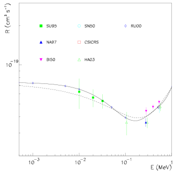
Figure 10: The low energy data and the fit of the auxiliary function $R(E)$ for the p + n $\leftrightarrow$ $\gamma$ + ²H reaction. The solid line is the overall best fit, the dashed curve is based only on experimental data. The theoretical points taken from [80] have a negligible error bar on this scale. The error bars for the experimental points also include the propagated uncertainty on the energies.

The fit of the $R(E)$ function is almost completely determined by the Rupak results. The reaction rate was calculated analytically according to Equation (3.18). Linear error propagation leads to an estimate of uncertainty $\leq$ 0.4% for $T_{9}\leq 1.5$.

Since the database was limited to $E\leq 1\,{\rm MeV}$, we expect that our rate will disagree with the previous estimates at high temperature; actually, starting from $T_{9}\sim 2$, with $T_{9}=T/10^{9}\,K$, the difference with respect to the rate published in [14] has almost a linear growth; the inclusion of higher energy data in an auxiliary fit ($\sim 3\div 6\,{\rm MeV}$) allows to check that $0.1\%$ variations appear from $T_{9}\sim 2$. For this reason we choose to use our rate in the range $T_{9}\leq 1.5$, where it is certainly more accurate, and matching it with the rate evaluated in [14], that is still used at higher temperatures $T_{9}\geq 1.5$. The overall uncertainty has been conservatively estimated as $1.2\%$ for $T_{9}\leq 1.5$, and includes the theoretical ($\leq 1\%$), the fitting ($\leq 0.18\%$), statistical ($\leq 0.4\%$) and normalization errors ($\sim 0.48\%$). The latter is due to the disagreement in the thermal capture cross sections [66]. The uncertainty grows to $\sim 8\%$ for $T_{9}>1.5$, being based on the error budget of [14] and the matching and normalization errors. For comparison, the analysis performed in [83] gives a sample variance error of $4.45\%$, while the uncertainty quoted in [19] is $2.5\%$. All the available rates agree at about 1 $\sigma$ or better within the quoted errors.

3.4.2 Reaction dp$\gamma$: ²H + p $\leftrightarrow$ $\gamma$ + ³He

.

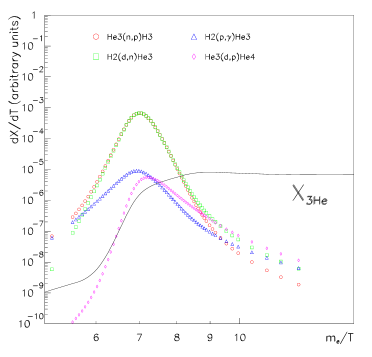
Figure 26: Leading processes for production and destruction of ³He.

It is one of the main responsible of the ³He synthesis both at high and low temperatures. When the deuterium formation channel is opening, this role is played instead by the strong reaction ddn, ²H + ² H $\leftrightarrow$ n + ³He (see Figure 26). The dp$\gamma$ is a direct capture reaction, for which it exists quite a recent theoretical model [84]. The data sets we consider are [18], [85]-[93]. Some discrepancies exist for the lower energies data, but in [90] the authors stress on the presence of a systematic error in their previous data (see e.g. [89]), with an upward correction that reduces the compatibility problem with the older data reported in [92]. Moreover, the latter data set by Griffiths is likely to be affected by a 10%-15% normalization error due to the wrong stopping powers used for the heavy-ice targets [91, 93], so that the disagreement is now reduced with respect to the first claims. Finally, the recent data from the LUNA collaboration [18] allow to firmly establish the low energy behavior of the astrophysical factor: for example, the older analysis performed in [83], not including them and with a less accurate treatment of the other experiments systematics gave a sample variance error of $13.2\%$, while our present study suggests an overall uncertainty for the rate less than 3%. In the recent compilation [19] the estimated error is close to 7%, but this number is dominated by the normalization error and so it is likely to be overestimated (see our discussion in Section 3.3). We get a data normalization spread of $\varepsilon\sim 1\%$.

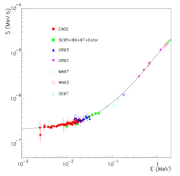
Figure 11: The data and fit for the astrophysical factor of ${{}^{2}H}+p\rightarrow\gamma+{{}^{3}He}$. The fit of $S(E)$ is with a cubic polynomial.

As in our previous work [20], the fit of all the data available has been performed with a cubic polynomial, and both the rate and uncertainty were obtained by numerical integrations, in fair agreement with the semi-analytical formula introduced in Section 3.2.2.

3.4.3 Reaction ddn: ²H + ²H $\leftrightarrow$ n + ³He

.

At $T_{9}\sim 1$, almost all ³He is produced through this typical Direct Interaction channel (see Figure 26). The energy range of main interest for the BBN is $0.01\div 2.5$ MeV, with a particular relevance of the values $E\leq 0.4\,{\rm MeV}$. Apart from some windows, the experimental situation for both the ddn and ddp (see later) reactions is quite good, if compared with other processes: they are strong interactions, their Coulomb barrier is low, and their relevance as thermonuclear fusion energy routes made their study quite appealing. Nevertheless their importance for BBN requires further efforts. We used the data [94]-[100]; note that the data of [101], used in [19], are only a preliminary report of the measurements quoted in [98], so they are not an independent data set and should be excluded. The data of [95] quite accurately fix the high energy behavior of this astrophysical factor, and the data in [98] allow to quote a normalization of the $S$ factor (and then of the rate) of 1.3%.

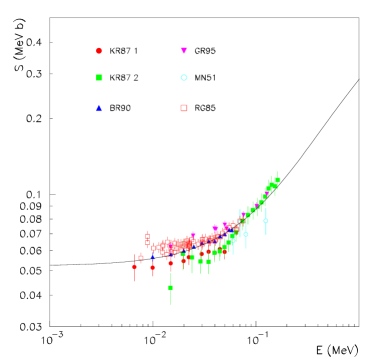
Figure 12: The data and fit for the $S$ factor of the ²H + ²H $\leftrightarrow$ n + ³He reaction.

As many data are available, and they are generally affected by a small normalization or overall uncertainties (at the level of few percent), even relatively low discrepancies on the scale and/or the behavior of the $S(E)$ will show up in the value of the reduced $\chi^{2}$, which is of the order of $10$ or greater at its minimum. Our method gives an overall uncertainty at the level of $1.3\%$, while for comparison the analysis performed in [83] gives a sample variance error of $3.1\%$. It should be pointed out that, while the uncertainty expected on the basis of the best determinations should be even lower, when combining several data sets the experimental situation suggests the presence of systematics. Indeed some experiments are likely to have underestimated the errors or could be affected by some unknown bias. In this situation, every regression method makes poor sense, and we continue to follow our approach just for consistency. As a confirmation of how difficult the analysis is in this case, we observe that the error budget estimated in a completely different approach in [19] is greater for the ddp ($\simeq 6.9\%$) than for the ddn($\simeq 5.5\%$) reaction, despite of the fact that the quality and the source of data are comparable, when not better and even more abundant for the first reaction.

As this reaction and the conjugate ddp strongly influence the ²H error budget, so that it affects many of the nuclides predictions, we strongly recommend a new experimental campaign to determine accurately (say at the 1% level) both the magnitude and shape of the $S(E)$ in the wide range useful for BBN studies (E$\leq$ 2.5 MeV), and in particular for $0.2\leq E\leq 1$ MeV, where actually no data presently exist.

3.4.4 Reaction ddp: ²H + ²H $\leftrightarrow$ p + ³H

.

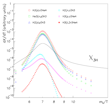
Figure 25: Leading processes for production and destruction of ³H.

This process is the leading source of direct tritium synthesis (see Figure 25). The discussion of its experimental situation closely follows our analysis of the previous reaction ddn, apart from the fact that very low energy data are available [100], which have to be corrected for screening effects in order not to bias the result. The data we used for this reaction are contained in the same References quoted for the ddn, as these processes are usually studied together. Since these two reactions are non-resonant, in both cases a polynomial fit for $S(E)$ is used, while the rates and errors were obtained by numerical integration. The uncertainty in the relevant temperature range is less than $1\%$.

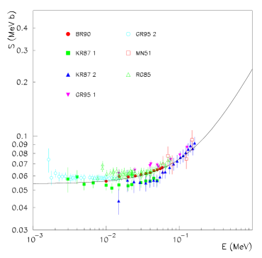
Figure 13: The data and fit for the $S$ factor of the ²H + ²H $\leftrightarrow$ p + ³H reaction.

3.4.5 Reaction tdn: ³H + ²H $\leftrightarrow$ n + ⁴He

.

The tdn is the fundamental channel for ⁴He synthesis during BBN. Many data are available for this process, also because it is the most promising process for the thermonuclear fusion research (low Coulomb barrier and high Q-value). Actually it is the energy production mechanisms considered for the next generation controlled fusion reactor, ITER [103]. A broad resonance in ⁵He, having $E_{R}=0.064$ MeV and $\Gamma=0.076{\pm}0.012$ MeV is superimposed to the non-resonant background. This allows to use a Breit-Wigner shape to extrapolate with some accuracy the $S$ factor also to energies below the range covered by the data. The data sets we used are [104]-[111], with the Conner data [105] excluded at energies greater than $240$ keV, where the isotropy assumption for $\sigma(E)$ fails. The rate and error estimate were both calculated numerically.

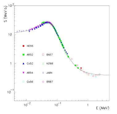
Figure 14: The $S(E)$ data and fit for the ³H + ²H $\leftrightarrow$ n + ⁴He channel

Our error estimate is $\simeq 0.6\%$, and $\varepsilon\sim 0.02$ (for a $\chi_{\nu}^{2}\simeq 1.4$), while for comparison the analysis performed in [83] gives a sample variance error of $\sim 4\%$, while the discrepancy error estimated in [19] is about of 2.2%.

3.4.6 Reaction he3dp: ³He + ²H $\leftrightarrow$ p + ⁴He

.

Like the conjugate reaction tdn, it is dominated by a broad ⁵He resonance, in this case at $\simeq 0.2$ MeV. There is quite a satisfactory experimental knowledge of this process, even if the dispersion of the data grows for $E\leq 0.2\,{\rm MeV}$, introducing some uncertainty on the resonance parameters. It is the second route to ⁴He production after the tdn reaction, but its indetermination mainly plays a role in the ³He and ⁷Li yields, as it essentially controls the burning of ³He. The data considered in our analysis are the ones reported in [112]-[125]; the two recent data sets [124, 125], firstly included in this compilation, once corrected for the screening effect allow for a better coverage of the low-energy region. Our new rate agrees within the errors with the rate published in [14], where the total error is estimated to be 8% (1 $\sigma$). For comparison, the analysis performed in [83] gives a sample variance error of 9.15%, while in [19] a 7.3% result is quoted. We estimate a rate uncertainty of the order of $0.6\%$, while $\varepsilon\sim 0.03$.

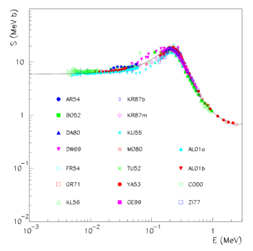
Figure 15: The $S(E)$ data and fit for the ³He + ²H $\leftrightarrow$ p + ⁴He reaction

3.4.7 Reaction he3np: ³He + n $\leftrightarrow$ p + ³H

.

This process keeps ³He and ³H in equilibrium at (relatively) high temperatures. During BBN it plays an important role in determining the final abundances of ³He and ⁷Li. In our regression we used the data reported in [126]-[130], by limiting the analysis to $E\leq 1{\rm MeV}$ as in [19]: this allows to cover the most interesting range for the BBN by significantly reducing the numbers of parameters needed to have a good fit. Thanks to the new measurements of the reverse reaction cross section near the threshold reported in [130] and to the accurate knowledge of the thermal capture rate [128], both the normalization and the shape of the $R(E)$ factor are well known, so that its contribution to the final error budget is low enough now not to require further measurements. In particular we find a statistical uncertainty of at most $0.2\%$, and a normalization spread of $\varepsilon\sim 0.002$.

Figure 16: The $S$ factor data and fit of the ³He + n $\leftrightarrow$ p + ³H.

3.4.8 Reaction be7np: ⁷Be + n $\leftrightarrow$ p + ⁷Li

.

It is the main responsible for ⁷Be/⁷Li conversion during the relevant phases of the BBN (in the final stage, the ⁷Be electron capture is actually more important). Only for very low energies, from $25\;{\rm meV}$ to $13.5$ keV, data are available on the direct process [131], while for higher energies one has to rely on the data for the reverse reaction [132, 133]. To avoid the introduction of significant errors due to the use of the detailed balance conversion near the threshold, we considered indirect data with energy $\geq 40$ keV only. As for the previous he3np reaction, we also restricted the analysis at energies $E\leq 2$ MeV, that are essentially the only ones relevant for BBN. However, differently than the non-resonant he3np reaction, whose rate was obtained analytically, this process has a resonance at $E\simeq 0.32$ MeV that suggests to use a fully numerical approach, both for the rate and the uncertainties. Note that despite of the few data set available, the Koeler data [131] fix the overall scale error to the $\simeq 2.1\%$ level, thus making this process quite accurately known for the purpose of BBN studies. The statistical error is of the order of $0.7\%$.

Figure 17: The $S$ factor data and fit of the ⁷Be + n $\leftrightarrow$ p + ⁷Li reaction.

3.4.9 Reaction $\alpha$he3$\gamma$: ⁴He + ³He $\leftrightarrow\gamma$ + ⁷Be

.

It is the dominant channel for direct ${{}^{7}Be}$ production and, in the (relatively) high-$\eta$ Universe suggested by WMAP data, practically all ⁷Li synthesis is controlled by this reaction. Its importance for the prediction of the solar neutrino spectra has motivated several theoretical and experimental efforts in the past years to obtain a better estimate of the cross section. A constant plus a decreasing exponential times a polynomial was used to fit its non-resonant $S$ factor, and the data used are [134]-[141], where the data in [137] were renormalized by a factor 1.4 to correct for the Helium gas density. Our regression method estimates an error of less than 3%, mainly dominated by the scale uncertainty. Both the value of the reduced $\chi^{2}$, $\chi_{\nu}^{2}=2.1$, and the high average renormalization we find from the fit, of the order of $20\%$, in agreement with the majority of the quoted errors, strongly suggest to undergo a new measurement campaign, to finally establish both the shape and the scale of this process at a few percent accuracy level. Of course the solar neutrino predictions would benefit of this new data, too.

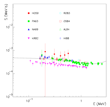
Figure 18: The $S$ factor fit and data for the ⁴He + ³He $\leftrightarrow$ $\gamma$ + ⁷Be reaction.

3.4.10 Reaction li7p$\alpha$: ⁷Li + p $\leftrightarrow$ ⁴He + ⁴He

.

This is the main process destroying ⁷Li during the BBN. The data used in our analysis are the ones quoted in [142]-[146]. A self-consistent correction for the screening potential was also performed, whose effect is particularly significant for the low-energy data of Engstler et al[145, 146]. Our estimate for the overall error is of the order of 2% in the relevant temperature range, while $\varepsilon\sim 0.01$.

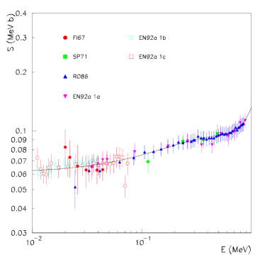
Figure 19: The data and fit for the $S$ factor of the ⁷Li + p $\leftrightarrow$ ⁴He + ⁴He reaction.

3.4.11 Reaction $\alpha$d$\gamma$: ⁴He + ²H $\leftrightarrow\gamma$ + ⁶Li

.

Even if it is a weak electric quadrupole transition, this reaction is important as represents the main ⁶Li production reaction. It is experimentally studied only at E $>$ 1 MeV and around the 0.711 MeV resonance. The low energy range is only weakly constrained by an upper limit, while the theoretical estimates for the non-resonant rate compiled in [15] show differences of $1\div 2$ orders of magnitude and were used to establish upper and lower limits. These features suggest the introduction of a temperature-dependent asymmetric uncertainty. It would be useful to get new data at E $\leq 0.6$ MeV in order to establish a reliable estimate of the standard BBN production of ⁶Li; in fact one cannot presently rule out the possibility that a relevant fraction of the observed ⁶Li in PopII stars has primordial origin (see [147] and our discussion in Section 4.1.5). In view of the serious lack of data, we simply updated the code with the inclusion of the NACRE evaluation for rate and errors.

3.4.12 Reaction li6phe3: ⁶Li + p $\leftrightarrow$ ³He + ⁴He

.

It is the main ⁶Li destruction channel. Available data for the cross section are quite abundant and accurate

We used the data [148]-[153] as well as those in References [143, 145], already cited for the li7p$\alpha$ process, with the last one self-consistently corrected for the screening effect. The estimated error is lower than $2\%$ and, quite negligibly contributing to the eventual accuracy of ⁶Li estimate, with respect to the one coming from the $\alpha$d$\gamma$ reaction. We estimate $\varepsilon\sim 0.09$.

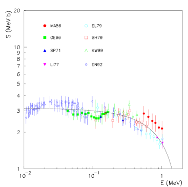
Figure 20: The data and fit for the $S$ factor of the ⁶Li + p $\leftrightarrow$ ³He + ⁴He reaction.

3.5 Main sub-leading processes

3.5.1 Reaction $\alpha$t$\gamma$: ⁴He + ³H $\leftrightarrow$ $\gamma$ + ⁷Li

.

This is the main channel for the direct synthesis of ⁷Li, and has been known since a long time as a crucial process for the ⁷Li predictions of the BBN (see [14]). However, especially thanks to the recent data of [154], its rate is relatively well known and, within the uncertainties, it only contributes at the percent level to the ⁷Li yield. This is one of the main consequences of the present suggested range for $\omega_{b}$, that indeed points out the leading role of the $\alpha$he3$\gamma$ reaction as the main route to A=7 elements production.

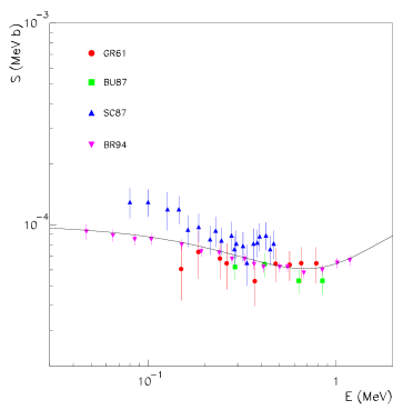
Figure 21: The data and fit for the $S$ factor of the ⁴He + ³H $\leftrightarrow$ $\gamma$ + ⁷Li reaction.

We parameterize the $S$ factor as in the case of the $\alpha$he3$\gamma$ reaction. The data used are [154]-[157], and our regression protocol gives $\chi_{\nu}^{2}\simeq 0.71$, with an overall uncertainty estimated at the level of 15% and $\varepsilon\sim 0.02$.

3.5.2 Reaction tp$\gamma$: ³H + p $\leftrightarrow$ $\gamma$ + ⁴He

.

This non-resonant process is the third one in order of importance involved in the ⁴He synthesis, but its influence on the final error budget of all nuclides is marginal. The $old$ rate for this reaction is that published in the compilation [12]. Meanwhile, new data were taken [158, 159], and a new fitting of the astrophysical $S$ factor is now available [159]

$$S(E)=S_{0}+S_{1}E+S_{2}E^{2}~{}~{}~{},$$ (3.55)

$$S_{0}=2.0{\pm}0.2\>keV\,mb~{}~{}~{},$$ (3.56)

$$S_{1}=(1.6{\pm}0.4){\times}10^{-2}\>mb~{}~{}~{},$$ (3.57)

$$S_{2}=(1.1{\pm}0.3){\times}10^{-4}\>mb/keV~{}~{}~{}.$$ (3.58)

We used these parameters to estimate the best rate, while its uncertainty is assumed to be $\Delta S(0)/S(0)\simeq 10\%$. Notice that correlations between the parameters haven’t been published, so our error propagation method on this rate cannot be used without a full re-analysis of the data.

3.5.3 Reaction li7p$\gamma$: ⁷Li + p$\stackrel{{{}^{8}{\rm Be}}}{{\longrightarrow}}\gamma$ + ⁴He + ⁴He

.

This reaction mainly proceeds trough the resonant term at $E_{8{\rm Be}}=19.86$ MeV, but also has a non-negligible non-resonant contribution. Both were quite recently re-determined in [160]. The relative importance of this reaction as an additional burning channel for the ⁷Li was pointed in [14], where its contribution was estimated to change the destruction rate up to $\sim$ 8% at $T_{9}=1$, but this seems to be neglected in all recent studies. Notice that the new data collected in [160] move upwards the estimate of the non-resonant contribution by more than a factor 10, thus further increasing its role. Tough sub-leading, it is worthwhile to note that within the actual uncertainties and assuming the WMAP range for $\omega_{b}$, this process acquires a role comparable to that of ⁷Li +p $\rightarrow$ ⁴He + ⁴He and ⁴He+³H$\rightarrow\gamma$+⁷Li reactions in determining the final prediction of ⁷Li. The data sets used in our analysis are [160]-[162]. We estimate an overall error of $3\%$ and a large value of the normalization spread parameter, $\varepsilon\sim 0.14$.

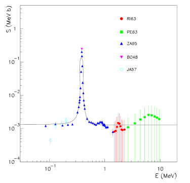
Figure 22: The data and fit for the $S$ factor for the ⁷Li + p $\leftrightarrow$ $\gamma$ + ⁸Be reaction.

3.5.4 Reaction be7n$\alpha$: ⁷Be + n $\leftrightarrow$ ⁴He + ⁴He

.

To our knowledge, evaluations for the rate of this reaction have only been published in [9] and [23], without information on the sources of the data and error estimate. We did not find further analysis in the following compilations by Fowler et al. [10]. The two data sets of the reverse process published in [163, 164] refer to center of mass energies of the direct one greater than 0.6 MeV, thus leaving a great uncertainty in the BBN window. They seem to be roughly consistent with the old estimate of the rate, and a new one in view of so scarce data would make little sense. For this reason we adopted Wagoner’s rate, assuming a factor 10 uncertainty, as he suggested as a typical conservative value. Within this allowed range, this reaction could play a non-negligible role in direct ⁷Be destruction, so it would be fruitful to have a new experimental determination. Apart from the role of unknown or little known ⁸Be resonances, it is however unlucky that the used extrapolation may underestimate the rate by more than one order of magnitude, as this process mainly proceeds through a p-wave.

3.5.5 Reaction li7dn$\alpha$: ⁷Li + ²H $\leftrightarrow$ n + ⁴He + ⁴He

.

The deuterium induced destruction processes of ⁷Li are dominated by this reaction, and a relatively recent analysis on this issue has been published in Reference [165]. However, within a conservatively assigned 50% uncertainty, the new evaluation produces almost no change in the Lithium amount with respect to the compilation [12], so it seems difficult that this process could play a role in reducing the $\sim 3\sigma$ discrepancy between predicted and observed ⁷Li yields.

3.5.6 Reaction be7dp$\alpha$: ⁷Be + ²H $\leftrightarrow$ p + ⁴He + ⁴He

.

The rate for this reaction is taken from [12], and is probably derived from the Parker estimate [166] based on the data published in [167]. It has been recently pointed out [168] that an enhancement of this process at low energies ($E_{CM}\leq 0.5\>{\rm MeV}$) of a factor $100$ or larger could reduce the discrepancy between the predicted and observed values of ⁷Li. Even if this possibility cannot be ruled out on the basis of the available data, we stress that there are no compelling reasons, both theoretical and experimental, suggesting such an anomalous enhancement at low energies. New measurements will greatly help in clarifying this issue.

4 Light nuclei abundances

In this Section we first review the present data on primordial abundances of light nuclides. The aim is to provide a sufficiently self-contained description of the issue, mainly collecting the most recent results more than entering into the complexity of the measurement procedures and of all possible sources of systematics. For this reason it should not be considered as a complete discussion on such an involved topic. More details on the experimental techniques can be found in the original papers we do quote in the following. The second part of this Section is then devoted to compare the theoretical expectations, obtained by numerically solving the BBN system of equations, with experiments. Particular stress is given to quantify uncertainties, in particular those due to propagation of nuclear rate measurement errors.

4.1 Experimental results

4.1.1 ²H

.

The deuterium is known to be the nuclide that better allows for a precise determination of the value of $\eta$. The most recent experimental results are discussed in [169], where the authors deduce the estimate

$$X_{{}^{2}{\rm H}}/X_{p}=(2.78^{+0.44}_{-0.38}){\cdot}10^{-5}~{}~{}~{}.$$ (4.1)

This value is the average of five measurements of DI/HI column ratio in different QSO absorption systems at high red-shift, obtained via deuterium isotopic shift from hydrogen. In particular this analysis takes advantage of the new detection towards Q1243+3047, based on an improved modeling of the continuum level, the Ly$\alpha$ forest and the velocity structure of the absorption, as well as on a better relative flux calibration.

In spite of the fact that the reduced $\chi^{2}$ is pretty large $\chi^{2}_{\nu}=4.1$, when using the set of QSO measurements considered in [169], so that unidentified systematics may be still affecting some of the data (correlations with the column density, local peculiar depletion, etc.), it is nevertheless interesting to note that the preferred range for $X_{{}^{2}{\rm H}}/X_{p}$ is in quite a good agreement with a standard BBN scenario with three neutrinos and WMAP result for $\omega_{b}$. We will come back to this point later.

4.1.2 ³He

.

The ³He could provide other constraints on the BBN scenario, but here the experimental study is complicated by the fact that a relevant contribution is expected from stellar destruction and production, making difficult to extrapolate the primordial abundance of this nuclide. Apart from Solar System measurements, ³He is usually detected through the 8.665 GHz spin flip transition of ³He⁺, but data are limited to (chemically evolved) galactic HII regions and planetary nebulae (for this issue, see [170] and References therein.) Assuming the simplest scenario of a typically limited stellar enrichment of ³He, the best observed system (S209 region) suggests $X_{{}^{3}{\rm He}}/X_{p}\leq(1.1{\pm}0.2){\cdot}10^{-5}$, while a more conservative limit based on a larger sample gives $X_{{}^{3}{\rm He}}/X_{p}\leq(1.9{\pm}0.6){\cdot}10^{-5}$. As discussed in [171], at the moment one cannot really consider the ³He as a strong “baryometer” because of the uncertainty on the role of stellar processing, the limited range in metallicity explored, and also the weaker dependence of $X_{{}^{3}{\rm He}}$ on $\eta$ with respect to $X_{{}^{2}{\rm H}}$. On the other hand, if combined with the increasing precision of the BBN predictions, and using the value of $\eta$ as determined by present and forthcoming CMB data, these observations could clarify several issues related to the Galactic Chemical evolution.

Finally, we note that the evidence collected till now for a sort of ‘plateau’ with respect to metallicity [170] and the order of magnitude of the observed abundance at least qualitatively support the idea of a common, primordial origin for the bulk of this nuclide abundance.

4.1.3 ⁴He

.

The value of $Y_{p}$ is usually derived by extrapolating to zero metallicity measurements done in dwarf irregular and blue compact galaxies (BCGs), that are among the least chemically evolved galaxies. The values obtained have a typically low statistical uncertainty (at the level of $0.002$, i.e. less than $1\%$) because of the large number of data, but are affected by several systematical uncertainties, whose origin has been considered in many recent works (see e.g. References [172, 173]). The estimate given in [174], based on a wide database and on a careful study of the chemical evolution of BCGs, is

$$Y_{p}=0.238{\pm}(0.002)_{stat}{\pm}(0.005)_{sys}~{}~{}~{},$$ (4.2)

while in the recent work [175] the authors quote

$$Y_{p}=0.2421{\pm}(0.0021)_{stat}~{}~{}~{},$$ (4.3)

when the linear regression is performed vs. O/H on a restricted, detailed-studied sample of galaxies. These observations are obtained with high signal-to-noise ratio, and a self-consistent approach on several He spectral lines was used in order to fit simultaneously as many parameters as possible. They also found that the typical size of the systematic errors is of the order of few percent, but the best estimate of the combined effect is at the $0.5\%$ level. Slightly higher values (from 0.243 to 0.247) are found neglecting some corrections, using a wider data sample, performing regression versus N/H, or finally using different Equivalent Widths (EWs).

Very recently, in [176] a new, detailed analysis of the budget of systematics in $Y_{p}$ was performed. With a different method and sample selection, this analysis of the same data of Izotov and Thuan gives $Y_{p}$ = $0.249{\pm}0.009$, quite different indeed, even if consistent within 1 $\sigma$. If we adopt the conservative range quoted in [176], (0.232 $\div$ 0.258), and viewing these bounds as a reasonable 2 $\sigma$ interval for $Y_{p}$, we have (mimicking a “1 $\sigma$” error)

$$Y_{p}=0.245{\pm}0.007~{}~{}~{},$$ (4.4)

which indeed is the value we will use to compare our theoretical results. Even if a knowledge of $Y_{p}$ at the level of 3% may seem quite satisfactory, in order to use ⁴He to bound possible BBN scenarios, it would be quite important to improve the $Y_{p}$ measurement accuracy at the level of the quoted statistical uncertainty, which requires a clear understanding of main sources of systematics.

We would briefly point out that other methods have been proposed to estimate $Y_{p}$, that hopefully could help in understanding the role of unknown systematics in the previous results. For example, in [177] and References therein, $Y_{p}$ is determined from indirect studies of Galactic Globular Clusters. The value they found $Y_{p}=0.250{\pm}(0.006)_{stat}{\pm}(0.019)_{sys}$ is still far from the required accuracy, but at the moment it is a promising contribution to clarify the debated issue of the primordial ⁴He determination. Finally in [178] a first attempt was made to determine $Y_{p}$ from CMB anisotropies data, but the 1 $\sigma$ confidence level $0.160<Y_{p}<0.501$ is still too broad.

4.1.4 ⁷Li

.

The role of possible depletion mechanisms of the Spite plateau found in PopII dwarfs halo stars in the seminal paper [179] by Spite & Spite, is still under debate. For example, the authors of [180] found evidence for a positive dependence of $X_{{}^{7}{\rm Li}}$ on metallicity, estimating

$$X_{{}^{7}{\rm Li}}/X_{p}=1.23{\pm}0.06^{+0.68}_{-0.32}~{}~{}~{},$$ (4.5)

at 95 $\%$ C.L., with uncertainty dominated by systematics effect. In other cases [181, 182, 183] a negative trend and/or a dispersion of the measurements around the plateau greater than the experimental error was suggested. A huge number of mechanisms has been invoked to explain such a ⁷Li depletion, among which rotational mixing, diffusion, stellar winds, etc (see e.g.[184] and References therein for an introduction to the current status of PopII stellar models). However, according to [185], these effects are second order, and a general consensus on the primordial origin of (at least) the bulk of the ⁷Li plateau has been achieved. The value quoted in [185] is the following

$$X_{{}^{7}{\rm Li}}/X_{p}=2.19^{+0.46}_{-0.38}~{}~{}~{}.$$ (4.6)

An important step is the recent check that other objects like the Globular Cluster NGC 6397 turn-off stars share essentially the same $X_{{}^{7}{\rm Li}}$ [185, 186], and even the troublesome observations in the globular cluster M92 reported in [187] seem to agree much better with other determinations in the reanalysis performed in [188] with a new temperature calibration.

At the moment, how to compare the extracted value of $X_{{}^{7}{\rm Li}}$ with the one obtained from the standard BBN scenario is still quite a problematic issue. As the only traditionally observed line is the 6708 Å doublet of the neutral Lithium (Li I) and the fraction of ionized Lithium (Li II) is estimated to be larger than $99.7\%$, a critical parameter for the extraction of A(Li)$\equiv\log_{10}(n_{{\rm Li}}/n_{{\rm H}})+12$ is the effective temperature of stellar atmospheres $T_{\rm eff}$. Other parameters as surface gravity, metallicity or microturbulence are much less important [186]. As $T_{\rm eff}$ is only estimated indirectly, recently it was also pointed out the possible bias in extracting the plateau abundance from one spectral line only. Actually when the subordinate line at 6104 Å is tentatively used, some disagreement is found, and values obtained for A(Li) could be high enough, A(Li)$\sim 2.5$, to reduce the discrepancy with BBN predictions (further details can be found in [189] and References therein).

As in previous studies, we do not use $X_{{}^{7}{\rm Li}}$ in our BBN likelihood analysis, waiting for a clearer understanding of possible systematics in stellar modeling. However, further efforts should be also devoted in trying to reduce the large theoretical uncertainty which is still affecting $X_{{}^{7}{\rm Li}}$, mainly by lowering the uncertainty on the leading reactions, ⁷Be + n $\leftrightarrow$ ⁴He + ⁴He, ⁴He + ³He $\leftrightarrow$ $\gamma+{{}^{7}}$Be, and ${}^{7}{\rm Be}$ + ${}^{2}{\rm H}$ $\leftrightarrow$ p + ${}^{4}{\rm He}$ + ${}^{4}{\rm He}$, which are responsible for a large fraction of the overall error on $X_{{}^{7}{\rm Li}}$. We will come back to this point in Section 4.2.3.

4.1.5 ⁶Li

.

Among the remaining light nuclides, the most abundant (for the best range for $\eta$) is ⁶Li, with $X_{{}^{6}{\rm Li}}/X_{p}\sim 10^{-14}$. One has to conclude that, in the more viable scenarios, there is no hope at the present for its detection. Actually, some positive measurements in halo stars at the level of ⁶Li/⁷Li$\simeq 0.05$ were obtained in the last decade [190], but they reflect the post-primordial production of this nuclide in Cosmic Ray spallation nucleosynthesis. This does not mean that this issue is unrelated to BBN studies; on the contrary, as discussed e.g. in [191], the study of the chemical evolution of the fragile isotopes of Li, Be and B could constraint the ⁷Li primordial yield, hopefully further clarifying the observational situation in the Spite Plateau. For example, the survival of such a (relatively) high fraction of ⁶Li in halo PopII stars severely limits the possible depletion factor for the more tightly bound ⁷Li.

4.2 Theoretical predictions and uncertainties

4.2.1 General considerations

.

The goal of a theoretical analysis of BBN is to obtain a reliable estimate of the nuclide abundances $X_{i}$ and of their uncertainties, once the best values and errors on the standard physics inputs are known. These inputs are

• $\tau_{n}$, the neutron lifetime;

• $G_{N}$, the Newton gravitational constant;

• $\eta$, the baryon to photon number density ratio;

• the nuclear rates.

The first two parameters are now known with a satisfactory accuracy [3]

$$\tau_{n} = 885.7{\pm}0.8\,s~{}~{}~{},$$ (4.7)

$$G_{\rm N} = 6.7087{\pm}0.0010{\cdot}\,10^{-39}\,GeV^{-2}~{}~{}~{}.$$ (4.8)

Until recently, BBN has been the only probe of $\eta$, and the best fitting with the observed abundances was used to guess its value plus some insights on neutrino or non-standard physics. Thanks to the precise determinations of $\omega_{b}$ obtained by the WMAP Collaboration results on CMB anisotropies, even $\eta$ is now independently known with an increasing precision, fixing the predictions of the standard scenario of BBN within a relatively narrow range. The value of the baryon parameter $\omega_{b}=\Omega_{b}h^{2}$ from CMB measurements is presently the following [1]

$$\omega_{b}=0.023{\pm}0.001~{}~{}~{}.$$ (4.9)

As these first three sources of error are independent and uncorrelated, one can easily work out the propagated uncertainty on each $X_{i}$, by adding in quadrature the three contributions.

The error matrix due to nuclear rate uncertainties are calculated as in our previous work [20]

$$\sigma_{ij}^{2}=\frac{1}{4}\sum_{k}[(X_{i}(\Gamma_{k}^{+})-X_{i}(\Gamma_{k}^{-})][(X_{j}(\Gamma_{k}^{+})-X_{j}(\Gamma_{k}^{-})]~{}~{}~{},$$ (4.10)

where the sum is over all reactions and with all other parameters set at their best values. The value $\Gamma_{k}^{\pm}$ is the average $\Gamma_{k}$ rate plus (minus) the estimated $1$ $\sigma$ uncertainty. Thus the contribution to the uncertainty on $X_{i}$ is given by

$$\sigma_{i}=\sqrt{\sigma_{ii}^{2}}~{}~{}~{},$$ (4.11)

and the correlation between $X_{i}$ and $X_{j}$

$$\rho_{ij}(\eta)=\frac{\sigma_{ij}^{2}(\eta)}{\sigma_{i}(\eta)\,\sigma_{j}(\eta)}~{}~{}~{}.$$ (4.12)

Being a generalization of the method described in [192], this approach avoids the use of (time consuming) Monte Carlo simulations, while it does not require the existence of the functionals $\lambda_{ij}(\eta)=\partial ln\,X_{i}/\partial ln\Gamma_{k}$. This means that it can be applied even to the case of asymmetric or temperature dependent errors, which indeed is the case for several process rates. The reliability of the method is supported by the Central Limit Theorem (at least when many reactions contribute to the error almost on the same level) and the fact that there is typically a linear relation between the $X_{i}$ and the parameters they depend on. Furthermore a direct comparison with Monte Carlo simulations results done in [192] shows that the method gives accurate results. We expect that this agreement is even improved for the typically smaller errors we found, and the allowance for the temperature-dependence of these quantities.

Apart from the inputs we have discussed so far, a BBN scenario does depend on several parameters which set a specific theoretical framework. As a main example, the eventual abundances of (mainly) ⁴He is influenced by the fact that extra particle species contribute to the overall energy density at the MeV temperature scale. This increases the value of the Hubble parameter, so that neutron to proton ratio freezes out at larger temperatures, where the neutron fraction is higher. It is customary to parameterize their contribution in terms of the effective number of extra degrees of freedom, $\Delta N$, defined as follows

$$\rho=\rho_{e,\gamma,\nu}+\rho_{B}+\frac{7}{8}\,\left(\frac{T_{\nu}}{T}\right)^{4}\,\Delta N\,\rho_{\gamma}~{}~{}~{},$$ (4.13)

where $\rho$ is the total energy density. Actually $\Delta N$ is a simple constant term for species which are fully relativistic at the BBN epoch, while it is a scale factor depending function otherwise: for example, for particles with mass much larger than MeV, $\Delta N$ increases proportionally to the scale factor. For the case of extra relativistic degrees of freedom decoupled from the electromagnetic plasma, the maximal allowed range $0.232\leq Y_{p}\leq 0.258$ quoted in [176] would constrain $-1.14\leq\Delta N\leq+0.73$ for $\omega_{b}=0.023$. Since $\Delta Y_{p}\simeq 0.013\Delta N$, a shift of 0.001 in $\omega_{b}$ would produce only a change of the order of 0.04 in the previous limits (see the Tables 3 and 4 and F).

In addition to $\Delta N$, light nuclei yields are in general sensitive to several parameters characterizing particle interactions or rather features of their distribution function. Most studied examples are the possible value of neutrino chemical potential [193] (for most recent bound on this parameter see for example [194, 20]), or neutrino lifetime (for a review on this issue see [6]).

In what follows we will consider only the minimal standard scenario. We therefore assume no extra parameter at all, and so all theoretical predictions for ²H, ⁴He and ⁷Li abundances are determined by the value of $\eta$. A careful study of this case seems to us of particular relevance since, as we mentioned already, the baryon to photon density is independently fixed by CMB anisotropy measurements, so there are no free parameters left. Comparing experimental result with theoretical expectations is therefore a clean test of consistency of the simplest BBN dynamics, based on our present understanding of fundamental interactions and of the cosmological model. It may also give useful hints to point out possible systematics in the experimental results reviewed in the previous Section.

To compare the present sensitivity to $\omega_{b}$ of BBN with the one of WMAP, we will also study how this parameter is constrained by observed nuclide abundances, i.e. leaving its value as the only free parameter to be fitted, rather than using the WMAP value prior. To do this, or more generally to bound the values of any other set of parameters of the kind discussed so far, the standard procedure is to construct a likelihood function

$${\cal L}(\eta)\propto\exp\left(-\chi^{2}(\eta)/2\right)$$ (4.14)

with

$$\chi^{2}(\eta)=\sum_{ij}[X_{i}(\eta)-X_{i}^{obs}]W_{ij}(\eta)[X_{j}(\eta)-X_{j}^{obs}]~{}~{}~{},$$ (4.15)

where the proportionality constant can be obtained by requiring normalization to unity, and with $W_{ij}(\eta)$ denoting the inverse covariance matrix

$$W_{ij}(\eta)=[\sigma_{ij}^{2}+\sigma_{i,exp}^{2}\delta_{ij}+\sigma_{ij,other}^{2}]^{-1}~{}~{}~{},$$ (4.16)

where $\sigma_{i,exp}$ is the uncertainty in experimental determination of nuclide abundance $X_{i}$ and by $\sigma_{ij,other}^{2}$ we denote the propagated squared error matrix due to all other input parameter uncertainties ($\tau_{n}$, $G_{\rm N}$, etc.).

4.2.2 Some remarks on $\eta$

.

There are two different way to parameterize the baryon content of the Universe today, which can be used interchangeably, namely $\eta$ and $\omega_{b}$. It is interesting to review the simple relationship between these two quantities, in order to asses how uncertainties propagate from one parameter to the other. It is straightforward to get

$$\omega_{b}=\rho_{b}\frac{8\pi G_{N}}{3(H_{0}/h)^{2}}=\frac{8\pi G_{N}m_{u}}{3(H_{0}/h)^{2}}\,\eta\,\frac{2\zeta(3)}{\pi^{2}}\,T_{\gamma 0}^{3}\,f~{}~{}~{},$$ (4.17)

where

$$f=\frac{\rho_{b}}{m_{u}n_{b}}\simeq\left[\frac{m_{H}}{m_{u}}-Y_{p}\left(\frac{m_{H}}{m_{u}}-\frac{m_{4He}}{4m_{u}}\right)\right]~{}~{}~{}.$$ (4.18)

This expression leads to

$$\eta{\cdot}10^{10}=273.49\,\omega_{b}\frac{1}{1-0.007\,Y_{p}}\bigg{(}\frac{6.707{\times}10^{-45}{\rm MeV}^{-2}}{G_{N}}\bigg{)}\bigg{(}\frac{2.725K}{T_{\gamma 0}}\bigg{)}^{3}~{}~{}~{}.$$ (4.19)

The uncertainties on the parameters ($Y_{p},G_{N},T_{\gamma 0}$) generate a $\Delta\eta/\eta$ at the level of $0.1\%$ (errors added in quadrature), which in view of the present determination of $\omega_{b}$, $\Delta\omega_{b}/\omega_{b}\sim 4\%$, is sub-leading and can be neglected in what follows.

As a further remark we recall that the value of $\eta$ lowers from early times to the end of nucleosynthesis, because of the entropy transfer to photons during $e^{\pm}$ annihilation phase. Typically [22] the final value $\eta_{f}$ is chosen as the input parameter, while the initial value, at $T\simeq 10\,{\rm MeV}$, is then deduced as

$$\eta_{i}=\eta_{f}\left(\frac{\bar{z}_{f}}{\bar{z}_{i}}\right)^{3}~{}~{}~{},$$ (4.20)

where we recall $\bar{z}=aT$. A careful estimate of this relation should take into account the mass of the electron even at initial condition, so that entropy is not simply proportional to $\bar{z}^{3}$. Furthermore the value of photon temperature $T$ get modified by the QED thermodynamical corrections to energy densities and pressures of $e^{\pm}$ and $\gamma$, as well as from the the small effects of the residual neutrino coupling to the electromagnetic plasma. Including all these one gets the estimate $\eta_{i}\simeq 2.73\eta_{f}$, slightly different than the simplest result one would get neglecting these effects, and which is for example used in [22], $\eta_{i}=2.75\eta_{f}$. Actually the corresponding corrections on the nuclide abundances are quite small. For $\omega_{b}=0.023$ we estimate

$$10^{5}\Delta X_{{}^{2}{\rm H}}/X_{p}=0.03,\,\,\Delta Y_{p}=-0.6{\times}10^{-4},\,\,,10^{10}\Delta X_{{}^{7}{\rm Li}}/X_{p}=-0.07~{}~{}~{},$$ (4.21)

In what follows $\eta$ always stands for $\eta_{f}$.

4.2.3 Results with the WMAP prior on $\omega_{b}$

.

nuclide $i$	central value	$\sigma_{ii}$	$\sigma_{\omega_{b}}$
$X_{{}^{2}{\rm H}}/X_{{\rm H}}$   ($10^{-5}$)	2.44	${\pm}0.04$	${}^{+0.19}_{-0.16}$
$X_{{}^{3}{\rm He}}/X_{{\rm H}}$  ($10^{-5}$)	1.01	${\pm}0.03$	${}^{+0.02}_{-0.03}$
$Y_{p}$	0.2481	${}^{+0.0002}_{-0.0001}$	${}^{+0.0004}_{-0.0004}$
$X_{{}^{6}{\rm Li}}/X_{{\rm H}}$   ($10^{-14}$)	1.1	${\pm}1.7$	${\pm}0.07$
$X_{{}^{7}{\rm Li}}/X_{{\rm H}}$   ($10^{-10}$)	4.9	${\pm}0.4$	${\pm}0.4$

Table 3: The light nuclide abundances for $\omega_{b}=0.023$ (second column). The (1 $\sigma$) uncertainties due to nuclear rates errors ($\sigma_{ii}$) and $\omega_{b}$ ($\sigma_{\omega_{b}}$) are also shown in the third and fourth columns, respectively.

As we mentioned, in the standard BBN scenario with no extra effective degrees of freedom or neutrino chemical potential, the light nuclide abundances are determined by the baryon density only. In Table 3 we report the values for the most relevant nucleosynthesis products, assuming the WMAP result, $\omega_{b}=0.023{\pm}0.001$. We also show the corresponding uncertainties due to the propagated errors $\sigma_{ii}$ on nuclear rates, as well as $\sigma_{\omega_{b}}$, the one induced by $\omega_{b}$ 1 $\sigma$ error. As a general comment on these results we can say that our analysis of experimental rates, and in particular the adopted method for error estimates, led to a sensible reduction of $\sigma_{ii}$ compared to our previous results in [20]. The reason for this is easily understood. In [20] we used a much more conservative approach, since we accounted for the fact that, for several rates, experimental results were often in disagreement by introducing a large maximal error defined similarly to the parameter $\varepsilon$ of Equation (3.54).

As we already mentioned in the Introduction the value of $\omega_{b}$ adopted in our analysis is the result given by the WMAP Collaboration combining their findings with those on CMB anisotropies of CBI and ACBAR experiments as well as with 2dFGRS data on power spectrum assuming a $\Lambda$CDM model. Slightly different values are obtained by including Lyman $\alpha$ forest data or introducing a running spectral index (see Tables 7 and 8 in [1]). In particular the best value for $\omega_{b}$ varies in the small range $0.022\div 0.024$ when combining different data sets, while the $1\sigma$ uncertainty is always of the order of $0.001$, or slightly smaller. The impact of these different determinations of $\omega_{b}$ on the nuclei abundance is shown in Table 4 where we report the best values for $\omega_{b}=0.022$, which is obtained combining WMAP+CBI+ACBAR in the running spectral index scenario [1], and for $\omega_{b}=0.024$, which is instead the preferred value of WMAP data only with a power law $\Lambda$CDM model. Notice that Deuterium and ⁷Li show appreciable changes, at the level of 10 %. We also note that the uncertainty due to nuclear rates, which in principle depends on the value of $\omega_{b}$, have very tiny variations and are still given by the values shown in the third column of Table 3. See also F where we report a fit of both nuclei abundances and the covariance matrix for ²H, ⁴He and ⁷Li.

nuclide $i$	$\omega_{b}=0.022$	$\omega_{b}=0.024$
$X_{{}^{2}{\rm H}}/X_{{\rm H}}$   ($10^{-5}$)	2.63	2.28
$X_{{}^{3}{\rm He}}/X_{{\rm H}}$  ($10^{-5}$)	1.03	0.98
$Y_{p}$	0.2477	0.2485
$X_{{}^{6}{\rm Li}}/X_{{\rm H}}$   ($10^{-14}$)	1.1	1.0
$X_{{}^{7}{\rm Li}}/X_{{\rm H}}$   ($10^{-10}$)	4.5	5.3

Table 4: The light nuclide abundances for $\omega_{b}=0.022$ (WMAP+ACBAR+CBI with a running spectral index) and $\omega_{b}=0.024$ (WMAP data only with a power law $\Lambda$CDM model).

Comparison with the analysis of [19] shows a similar trend, though the uncertainties quoted in [19] are typically larger for the reasons discussed in Section 3.3. As a main exception we mention the fact that we perfectly agree on the uncertainty quoted for $Y_{p}$, since in this case (almost) all error is due to neutron lifetime statistical uncertainty.

We now consider in more details our results for each nuclide.

• ²H –

  The Deuterium abundance is in quite a good agreement with the experimental result quoted in Section 4.1.1. This is perhaps the main indication that indeed the standard picture of BBN is fully satisfactory. We know in fact that ²H is extremely sensitive to the value of baryon density. Thus it is rather remarkable that the value found for $\omega_{b}$ from a completely independent observable, such as the CMB anisotropies, leads to a ²H yield very close (1 $\sigma$) to measurements.

  In our findings the uncertainty due to nuclear rates is now reduced to $1.6\%$, mainly because of our analysis of the two leading reactions ddn and ddp. It is interesting in fact to study the contribution of each rate to the total error $\sigma_{{}^{2}{\rm H}^{2}{\rm H}}$. The results are reported in Table 5.

  rate	$\delta\sigma_{{}^{2}{\rm H}^{2}{\rm H}}^{2}/\sigma_{{}^{2}{\rm H}^{2}{\rm H}}^{2}(\%)$
  dp$\gamma$	49
  ddn	37
  ddp	14

  Table 5: The contribution of reaction rate errors to the total (squared) uncertainty on $X_{{}^{2}{\rm H}}/X_{p}$

  The role of ddn and ddp is now of the order of $50\%$, while in our previous study it was largely dominant [20]. The reduced estimated uncertainties on these two processes, which are very efficient ²H burning channels, is mainly responsible for that. Notice that ²H uncertainty is now dominated by $\sigma_{\omega_{b}}$. Even more than in the past, the role of ²H as a baryometer is clearly established.

• ³He –

  The estimated value for ³He almost saturates the bound reported in Section 4.1.2, $X_{{}^{3}{\rm He}}/X_{p}\leq(1.1{\pm}0.2){\cdot}10^{-5}$, while is a factor two smaller than the conservative limit, $X_{{}^{3}{\rm He}}/X_{p}\leq(1.9{\pm}0.6){\cdot}10^{-5}$. It would be of great impact for standard BBN, as well as for theories on galactic chemical evolution, to have further experimental information on the abundance of this nuclide, trying to reduce the present bound. The error budget study shows that the theoretical uncertainty is equally shared by the nuclear rate errors and the uncertainty on $\omega_{b}$. Actually it is worth stressing that the value of the error due to nuclear rates is very close to what is found for ²H. It receives the main contributions from the processes he3dp and dp$\gamma$, as can be read from Table 6. On the other hand the fact that ³He is less critically depending on $\omega_{b}$ with respect to ²H shows up in a relatively smaller value of $\sigma_{\omega_{b}}$.

  rate	$\delta\sigma_{{}^{3}{\rm He}^{3}{\rm He}}^{2}/\sigma_{{}^{3}{\rm He}^{3}{\rm He}}^{2}(\%)$
  he3dp	80.7
  dp$\gamma$	16.8
  ddp	1.3
  ddn	1.2

  Table 6: The contribution of reaction rate errors to the total (squared) uncertainty on $X_{{}^{3}{\rm He}}/X_{p}$

• ⁴He –

  The value of the Helium mass fraction parameter is in very good agreement with previous theoretical determinations (see for example [19], [20], [195]). Comparison with the experimental values only shows a satisfactory agreement if we adopt the conservative estimate discussed in Section 4.1.3. The value given by [174] (see Equation 4.2) is instead compatible at the 3-$\sigma$ level, even considering their estimate of systematic error in the measurement. Similarly the result of [175] reported in Equation 4.3 is significantly lower with respect to the theoretical value. If we assume that Deuterium results points towards the consistency of both standard BBN and the WMAP result on $\omega_{b}$, we are led to the conclusion that the uncertainty of present measurements of $Y_{p}$ is largely dominated by systematic effects, which lead to an underestimation of ⁴He density. Of course a better agreement between data and theoretical estimates is obtained in less conservative theoretical frameworks with exotic physics like the presence of extra particles or large chemical potentials. These scenarios have been recently studied in [194], [195] and [20].

  rate	$\delta\sigma_{{}^{4}{\rm He}^{4}{\rm He}}^{2}/\sigma_{{}^{4}{\rm He}^{4}{\rm He}}^{2}(\%)$
  wnp	98.5
  ddn	1
  ddp	0.25
  dn$\gamma$	0.25

  Table 7: The contribution of reaction rate errors to the total (squared) uncertainty on $Y_{p}$

  We show in Table 7 the main contribution of rate uncertainties to the squared error $\sigma_{{}^{4}{\rm He}^{4}{\rm He}}$. We see in this case again how the new estimate for ddn and ddp uncertainties has lowered their role in the theoretical uncertainties on light nuclides. For ⁴He this uncertainty is now almost entirely due to neutron lifetime error. This is also the finding of [19].

• ⁶Li –

  The best estimate of ⁶Li, $X_{{}^{6}{\rm Li}}/X_{p}=1.1{\cdot}10^{-14}$ gives for the ratio ${}^{6}{\rm Li}/^{7}{\rm Li}$ the result $0.22{\cdot}10^{-4}$, well below the result obtained for this ratio in halo stars, which, as discussed in Section 4.1.5, is three order of magnitude larger. Theoretical uncertainty on this nuclide is still very large, at the level of $100\%$, and is entirely due to the effect of $\alpha$d$\gamma$, whose rate is still quite poorly known (see Section 3.4).

• ⁷Li –

  There are several reactions contributing to the total uncertainty for this nuclide, as shown in Table 8. Leading contributions to the $8\%$ error on the theoretical estimate for $\omega_{b}=0.023$ comes from be7n$\alpha$, he4he3$\gamma$ and be7dp$\alpha$. ⁷Li still has the largest theoretical error among the observed nuclides, of the same order of the one induced by $\omega_{b}$ uncertainty. In view of this it is worth stressing that new experimental results in particular on the be7n$\alpha$ and he4he3$\gamma$ would be extremely important. However, unless unexpected new data will change the present picture of the main production and destruction channels for this nuclide, it seems quite hard to reconcile the theoretical result with the experimental data, which are smaller by a factor $2\div 3$. This difference is at the level of $4\,\sigma$, more severe than in our previous analysis in [20] because of the different treatment of nuclear rate errors, and is possibly an evidence for POPII star atmospheric Lithium depletion.

  rate	$\delta\sigma_{{}^{7}{\rm Li}^{7}{\rm Li}}^{2}/\sigma_{{}^{7}{\rm Li}^{7}{\rm Li}}^{2}(\%)$
  be7n$\alpha$	40.9
  he4he3$\gamma$	25.1
  be7dp$\alpha$	16.2
  he3dp	8.6
  dp$\gamma$	4.0
  be7np	2.7
  ddn	1.8
  others	0.7

  Table 8: The contribution of reaction rate errors to the total (squared) uncertainty on $X_{{}^{7}{\rm Li}}/X_{p}$

4.2.4 Results for $\omega_{b}$ from ²H and ⁴He

.

We now study how the value of $\omega_{b}$ is constrained by standard BBN alone, without using the WMAP results for this parameter, but rather determining its best value and uncertainty from light nuclide abundances only. The aim of this analysis is to compare the present capability of BBN to fix the baryon content of the observable Universe with respect to that of CMB anisotropies. We consider two different analysis. We first use the ²H abundance only, to check the role of deuterium as a good baryometer. To this aim we construct the likelihood function

$${\cal L}\propto\exp\left[-\left(X_{{}^{2}{\rm H}}(\omega_{b})-X^{obs}_{{}^{2}{\rm H}}\right)^{2}W_{{}^{2}{\rm H}^{2}{\rm H}}(\omega_{b})/2\right]~{}~{}~{},$$ (4.22)

where notation has been described in Section 4.2.1. Using the QSO averaged result reported in (4.1) the best fit value and 68% C.L. uncertainty are found to be $\omega_{b}=0.021{\pm}0.002$. Notice that $W_{{}^{2}{\rm H}^{2}{\rm H}}(\omega_{b})$ is dominated by the experimental uncertainty in QSO measurements. Improved experimental measurements of ²H abundance would correspond to a more refined determination of $\omega_{b}$, since the role of theoretical uncertainty due to nuclear rate errors is presently quite small.

Figure 23: The $\omega_{b}$ determination using different cosmological observables. We report the likelihood function for WMAP result on CMB anisotropies (full line), ²H measurement (dashed line) and ⁴He analysis (dotted line).

A similar analysis can be performed using ⁴He. In this case we get $\omega_{b}=0.016^{+0.026}_{-0.009}$, at 68 % C.L., which is not very constraining in view of the generous uncertainty we have adopted for the experimental error on $Y_{p}$.

A comparison of all results is shown in Figure (23), where we report the likelihood profiles for the two determination of $\omega_{b}$ from ²H and ⁴He, as well as the one by WMAP. We read from this figure that indeed CMB anisotropies presently measure $\omega_{b}$ with the best accuracy, though ²H is also able to fix its values with a comparable precision. We are confident that the big effort performed by many groups in refining the theoretical modeling of BBN, along with new data and a better understanding of systematics may lead to a more accurate estimate of this important cosmological parameter by BBN alone. In this case comparison with present and very accurate determination from CMB experiments such as PLANCK will represent a precision test of the cosmological model describing the evolution of the Universe.

5 Conclusions

In this paper we have studied in details the results of standard primordial nucleosynthesis in view of the fact that baryon density is now independently measured using the Cosmic Microwave Background anisotropies. The WMAP Collaboration result for $\omega_{b}$, with its 4% accuracy, represents indeed an important step toward a detailed understanding of nuclide formation in the early Universe. Fixing the value of $\omega_{b}$ in fact implies that standard BBN scenario becomes a parameter free model, and comparison of theoretical expectations with data is therefore particularly significant.

Much effort have been done in the recent years by several groups in order to increase the level of accuracy of theoretical prediction on nuclide abundances, in particular by improving the estimate of the neutron to proton weak conversion rates, and the nuclear rate network. We think that the present paper represents a further contribution along this line, and we here summarize the main results of our study.

We have considered in great details the $n-p$ weak rates, which are responsible for neutron/proton chemical equilibrium, including the effect of distortion of neutrino distribution and QED effects. These rates are now known with a great accuracy, at the level of $0.1\%$. This result is now quite well established, and compatible results have been obtained by several groups, as we mentioned in Section 3. The main benefit of all these studies is that we presently have a remarkably accurate estimate of ⁴He mass fraction, which is mainly depending on the value of the neutron density at freeze out of weak reactions.

We have critically reviewed the whole set of nuclear reaction rates, and we have reported a detailed analysis of the main rates contributing to nuclide formation, as well as some sub-leading channels which, however, in view of their large uncertainty, may still play a role in BBN. Similar studies have appeared in the recent literature [19, 21] which as the present paper largely benefit of the NACRE Collaboration database. Our main goal has been to get a consistent data regression method, which may be also applied to all cases where data shows a clear evidence for systematic errors, and which can also account for correlations among data belonging to the same data set without introducing the bias discussed in [65].

Our study of the main nuclear reaction rates and their corresponding uncertainties has been used to quantify their contribution to the total error on the estimate of light nuclides, in particular ²H, ³He, ⁴He, ⁶Li and ⁷Li. With our present regression method typically the role of nuclear rate uncertainty is now smaller than in previous analysis [14, 19, 20] and is comparable or smaller than the corresponding uncertainty due to the present $\omega_{b}$ error. It is remarkable that indeed for ²H this improvement is particularly relevant. Refined experimental measurements of the ratio $X_{{}^{2}{\rm H}}/X_{p}$ as well as of the baryon fraction from CMB anisotropies would be a clean test of consistency of standard BBN. Primordial ⁶Li, whose theoretical estimate is still affected by a very large error of the order of $100\%$, is not presently measured, since it is likely that the observed value in POPII halo stars is due to cosmic ray spallation nucleosynthesis.

The ⁴He mass fraction uncertainty is estimated at the level of $0.1\%$, and is almost completely due to the neutron lifetime error. The nuclear rate uncertainties of the leading ddn, ddp and dn$\gamma$ processes contribute in fact for only $1.5\%$ of the total theoretical uncertainty for $\omega_{b}=0.023$.

The ⁷Li estimate is still affected by an order $10\%$ uncertainty mainly due to the role of the reactions be7n$\alpha$, he4he3$\gamma$ and be7dp$\alpha$. Further experimental results on these rates would be therefore highly desirable. In particular a better measurement of the he4he3$\gamma$ channel would also have important implications on the estimate of solar neutrino flux.

Apart from these processes, the BBN uncertainty budget is dominated by the effect of ddn, ddp and dp$\gamma$, which largely contribute to both ²H and ³He error, he3dp which represents the main source of uncertainty for ³He, and finally the $\alpha$d$\gamma$ process, which is entirely responsible for the large ⁶Li theoretical error.

The theoretical estimates for standard BBN with experimental determinations of ²H, ⁴He and ⁷Li show several interesting features. First of all it is remarkable that the value found for ²H for the WMAP best estimate of $\omega_{b}$ is in quite a good agreement with the results of QSO measurements, since they are compatible at 1 $\sigma$ level. The value found in the same scenario for $Y_{p}$ is instead slightly larger than what expected from present data, though agreement is found at 1 $\sigma$ level if we adopt a conservative estimate of the uncertainty, as in [176], largely dominated by systematics. The fact that the theoretical uncertainty for $Y_{p}$ is very small has important consequences in this respect. New experimental campaigns aimed to detect $Y_{p}$ and in particular a further effort to identify sources of systematics will clearly tell us if the standard BBN scenario is a satisfactory description or rather we have to consider more exotic possibilities.

Further constraints on this may come from future experimental measurements of ³He, which may be an independent way of fixing the baryon density. Finally, despite of the fact that ⁷Li theoretical predictions is still affected by a $10\%$ error, nevertheless there is a clear indication of a possible depletion mechanism which lowers the primordial abundance down to the value measured with Spite plateau. A different picture might emerge if new experimental results on some key reaction, as for example the be7dp$\alpha$ suggested in [168], will change our present understanding of the hierarchy of the nuclear processes contributing to light nuclide production in the early Universe.

Appendix A

BBN reaction network

We report in this Appendix the full list of reactions adopted in our numerical study of BBN responsible for the synthesis or the destruction of the $A\leq 7$ nuclides.

Weak Processes.

Name	Reaction
wnp	n $\leftrightarrow$ p
h3	3H $\rightarrow$ $\bar{\nu}_{e}$ + $e^{-}$ + 3He
be7	7Be + $e^{-}$ $\rightarrow$ $\nu_{e}$ + 7Li

(n,$\gamma$) Reactions

Name	Reaction
pn$\gamma$	p + n $\leftrightarrow$ $\gamma$ + 2H
dn$\gamma$	2H + n $\leftrightarrow$ $\gamma$ +3H
he3n$\gamma$	3He + n $\leftrightarrow$ $\gamma$ + 4He
li6n$\gamma$	6Li + n $\leftrightarrow$ $\gamma$ + 7Li
li7n$\gamma$	7Li + n $\leftrightarrow$ $\gamma$ + 8Li

(p,$\gamma$) Reactions

Name	Reaction
dp$\gamma$	2H + p $\leftrightarrow$ $\gamma$ + 3He
tp$\gamma$	3H + p $\leftrightarrow$ $\gamma$ + 4He
li6p$\gamma$	6Li + p $\leftrightarrow$ $\gamma$ + 7Be
li7p$\gamma$	7Li + p $\leftrightarrow$ $\gamma$ + 8Be
be7p$\gamma$	7Be + p $\leftrightarrow$ $\gamma$ + 8B

(d,$\gamma$) Reactions

Name	Reaction
dd$\gamma$	2H + 2H $\leftrightarrow$ $\gamma$ + 4He
$\alpha$d$\gamma$	4He + 2H $\leftrightarrow$ $\gamma$ + 6Li
li7d$\gamma$	7Li + 2H $\leftrightarrow$ $\gamma$ + 9Be

(t,$\gamma$) and (³He,$\gamma$) Reactions

Name	Reaction
he3t$\gamma$	3He + 3H $\leftrightarrow$ $\gamma$ + 6Li
$\alpha$t$\gamma$	4He + 3H $\leftrightarrow$ $\gamma$ + 7Li
$\alpha$he3$\gamma$	4He + 3He $\leftrightarrow$ $\gamma$ + 7Be
li6t$\gamma$	6Li + 3H $\leftrightarrow$ $\gamma$ + 9Be
be7t$\gamma$	7Be + 3H $\leftrightarrow$ $\gamma$ + 10B
li7he3$\gamma$	7Li + 3He $\leftrightarrow$ $\gamma$ + 10B

($\alpha,\gamma$) Reactions

Name	Reaction
li6$\alpha\gamma$	6Li + 4He $\leftrightarrow$ $\gamma$ + 10B
li7$\alpha\gamma$	7Li + 4He $\leftrightarrow$ $\gamma$ + 11B
be7$\alpha\gamma$	7Be + 4He $\leftrightarrow$ $\gamma$ + 11C

Charge exchange reactions

Name	Reaction
he3np	3He + n $\leftrightarrow$ p + 3H
be7np	7Be + n $\leftrightarrow$ p + 7Li

²H Stripping/Pickup (S/P) Reactions

Name	Reaction
ddn	2H + 2H $\leftrightarrow$ n + 3He
ddp	2H + 2H $\leftrightarrow$ p + 3H
tdp	3H + 2H $\leftrightarrow$ n + 4He
he3dp	3He + 2H $\leftrightarrow$ p + 4He
li6dn	6Li + 2H $\leftrightarrow$ n + 7Be
li6dp	6Li + 2H $\leftrightarrow$ p + 7Li
li8pd	8Li + p $\leftrightarrow$ 2H + 7Li
b8nd	8B + n $\leftrightarrow$ 2H + 7Be

³H and ³He S/P Reactions

Name	Reaction
li6nt	6Li + n $\leftrightarrow$ 3H + 4He
li6phe3	6Li + p $\leftrightarrow$ 3He + 4He
he3td	3He + 3H $\leftrightarrow$ 2H + 4He
li6td	6Li + 3H $\leftrightarrow$ 2H + 7Li
li6he3d	6Li + 3He $\leftrightarrow$ 2H + 7Be
li6tp	6Li + 3H $\leftrightarrow$ p + 8Li
b8nhe3	8B + n $\leftrightarrow$ 3He + 6Li
li7tn	7Li + 3H $\leftrightarrow$ n + 9Be
li7he3p	7Li + 3He $\leftrightarrow$ p + 9Be
be7tp	7Be + 3H $\leftrightarrow$ p + 9Be
li8dt	8Li + 2H $\leftrightarrow$ 3H + 7Li
b8dhe3	8B + 2H $\leftrightarrow$ 3He + 7Be

⁴He Pickup Reactions

Name	Reaction
be7n$\alpha$	7Be + n $\leftrightarrow$ 4He + 4He
li7p$\alpha$	7Li + p $\leftrightarrow$ 4He + 4He
be9p$\alpha$	9Be + p $\leftrightarrow$ 4He + 6Li
b10n$\alpha$	10B + n $\leftrightarrow$ 4He + 7Li
b10p$\alpha$	10B + p $\leftrightarrow$ 4He + 7Be
li6d$\alpha$	6Li + 2H $\leftrightarrow$ 4He + 4He
be9d$\alpha$	9Be + 2H $\leftrightarrow$ 4He + 7Li
be7t$\alpha$	7Be + 3H $\leftrightarrow$ 4He + 6Li
li7t$\alpha$	7Li + 3He $\leftrightarrow$ 4He + 6Li
b8t$\alpha$	8B + 3H $\leftrightarrow$ 4He + 7Be
li8he3$\alpha$	8Li + 3He $\leftrightarrow$ 4He + 7Li
be9d$\alpha$	9Be + 2H $\leftrightarrow$ 4He + 7Li

Ingoing 2-body Reactions.

Name	Reaction
ttnn	3H + 3H $\leftrightarrow$ n + n + 4He
he3tnp	3He + 3H $\leftrightarrow$ p + n + 4He
he3he3pp	3He + 3He $\leftrightarrow$ p + p + 4He
li7dn$\alpha$	7Li + 2H $\leftrightarrow$ n + 4He + 4He
be7dp$\alpha$	7Be + 2H $\leftrightarrow$ p + 4He + 4He
li7he3d$\alpha$	7Li + 3He $\leftrightarrow$ 2H + 4He + 4He
be7td$\alpha$	7Be + 3H $\leftrightarrow$ 2H + 4He + 4He
li7tnn$\alpha$	7Li + 3H $\leftrightarrow$ n + n + 4He + 4He
be7tpn$\alpha$	7Be + 3H $\leftrightarrow$ p + n + 4He + 4He
li7he3np$\alpha$	7Li + 3He $\leftrightarrow$ n + p + 4He + 4He
be7he3pp$\alpha$	7Be + 3He $\leftrightarrow$ p + p + 4He + 4He

Ingoing 3-body Reactions.

Name	Reaction
pnnd	p + n + n $\leftrightarrow$ n + 2H
ppnd	p + p + n $\leftrightarrow$ p + 2H
pnn$\gamma$	p + n + n $\leftrightarrow$ $\gamma$ + 3H
ppn$\gamma$	p + p + n $\leftrightarrow$ $\gamma$ + 3He
pn$\alpha\gamma$	p + n + 4He $\leftrightarrow$ $\gamma$ + 6Li

Appendix B

Graphical analysis reaction rates

A qualitative understanding of the role of each nuclear reaction to the creation/destruction of a definite light nuclide $i$ can be grasped by looking at the temperature behavior of their contribution to the right hand side of the corresponding Boltzmann equation for $X_{i}$. To this end we collect in this Appendix the log-log plots of the combinations

$$\Gamma_{kl\rightarrow ij}\,\frac{X_{l}^{N_{l}}\,X_{k}^{N_{k}}}{N_{l}!\,N_{k}!}~{}~{}~{},$$ (B.1)

versus $T_{9}=T/10^{9}\,K$, see (2.7). Baryon density is chosen as $\omega_{b}=0.023$. We show results only for those processes which contribute to change $X_{i}$ at leading level or for some interesting sub-leading reaction.

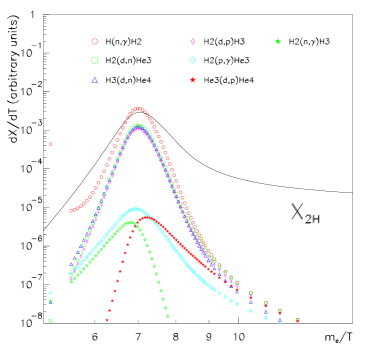
Figure 24: Leading processes for production and destruction of ²H.

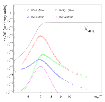
Figure 27: Leading processes for production and destruction of ⁴He.

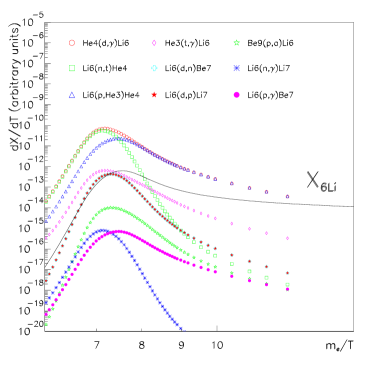
Figure 28: Leading processes for production and destruction of ⁶Li.

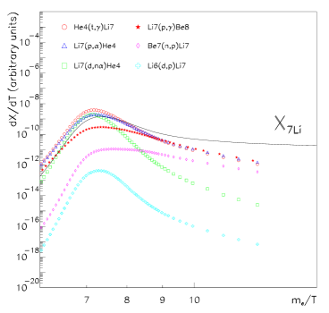
Figure 29: Leading processes for production and destruction of ⁷Li.

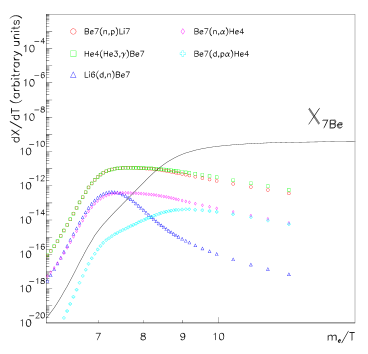
Figure 30: Leading processes for production and destruction of ⁷Be.

Appendix C

Fits of $n\leftrightarrow p$ weak rates

The neutron/proton weak rates have been fitted as function of $z=m_{e}/T$ with accuracy better than $0.06\%$ with the following expressions

$$\omega(n\rightarrow p) = \frac{1}{\tau_{n}^{ex}}\exp\left(-q_{np}/z\right)\,\sum_{l=0}^{13}a_{l}~{}z^{-l},\,\,\,\,\,\,\,\,\,\,0.01\leq T/{\rm MeV}\leq 10$$ (C.1)

$$\omega(p\rightarrow n) = \left\{\begin{array}[]{cc}\frac{1}{\tau_{n}^{ex}}\exp\left(-q_{pn}z\right)\,\sum_{l=1}^{10}b_{l}~{}z^{-l}&0.1\leq T/{\rm MeV}\leq 10\\ 0&0.01\leq T/{\rm MeV}<0.1\end{array}\right.$$ (C.4)

with

$$\begin{array}[]{lll}a_{0}=1&a_{1}=0.15735&a_{2}=4.6172\\ a_{3}=-0.40520{\cdot}10^{2}&a_{4}=0.13875{\cdot}10^{3}&a_{5}=-0.59898{\cdot}10^{2}\\ a_{6}=0.66752{\cdot}10^{2}&a_{7}=-0.16705{\cdot}10^{2}&a_{8}=3.8071\\ a_{9}=-0.39140&a_{10}=0.023590&a_{11}=-0.83696{\cdot}10^{-4}\\ a_{12}=-0.42095{\cdot}10^{-4}&a_{13}=0.17675{\cdot}10^{-5}&q_{np}=0.33979~{}~{}~{},\\ \\ b_{0}=-0.62173&b_{1}=0.22211{\cdot}10^{2}&b_{2}=-0.72798{\cdot}10^{2}\\ b_{3}=0.11571{\cdot}10^{3}&b_{4}=-0.11763{\cdot}10^{2}&b_{5}=0.45521{\cdot}10^{2}\\ b_{6}=-3.7973&b_{7}=0.41266&b_{8}=-0.026210\\ b_{9}=0.87934{\cdot}10^{-3}&b_{10}=-0.12016{\cdot}10^{-4}&q_{pn}=2.8602~{}~{}~{}.\end{array}$$ (C.15)

(C.16)

Appendix D

Fits of the S/R factors for the leading reactions

In this Appendix we report our fits of the S or R factor for each leading reaction and the largest energy $E_{Max}$ for which the fit is valid.

1. Reaction pn$\gamma$ : $p+n\leftrightarrow\gamma+{{}^{2}H}$

   $$R(E) = (7.31638{\cdot}10^{-20}+2.35455{\cdot}10^{-20}\,E^{\frac{1}{2}}-1.55683{\cdot}10^{-18}\,E$$ (D.1)

   $$+ 5.93351{\cdot}10^{-18}\,E^{\frac{3}{2}}-9.25443{\cdot}10^{-18}\,E^{2}+6.6732{\cdot}10^{-18}\,E^{\frac{5}{2}}$$

   $$- 1.82393{\cdot}10^{-18}\,E^{3})~{}cm^{3}s^{-1}$$

   $$[E_{Max} = 1\,MeV]$$

   
   

2. Reaction dp$\gamma$ : ${{}^{2}H}+p\leftrightarrow\gamma+{{}^{3}He}$

   $$S(E) = (0.214{\cdot}10^{-6}+0.556{\cdot}10^{-5}\,E+0.551{\cdot}10^{-5}\,E^{2}$$ (D.2)

   $$- 0.157{\cdot}10^{-5}\,E^{3})~{}MeV~{}b$$

   $$[E_{Max} = 2\,MeV]$$

   
   

3. Reaction ddn : ${{}^{2}H}+{{}^{2}H}\leftrightarrow n+{{}^{3}He}$

   $$S(E) = (0.0522+0.370\,E-0.196\,E^{2}+0.0672\,E^{3}-0.00885\,E^{4})~{}MeV~{}b$$ (D.3)

   $$[E_{Max} = 3.1\,MeV]$$

   
   

4. Reaction ddp : ${{}^{2}H}+{{}^{2}H}\leftrightarrow p+{{}^{3}H}$

   $$S(E) = (0.0542+0.205\,E-0.0240\,E^{2})~{}MeV~{}b$$ (D.4)

   $$[E_{Max} = 3.1\,MeV]$$

   
   

5. Reaction tdn : ${{}^{3}H}+{{}^{2}H}\leftrightarrow n+{{}^{4}He}$

   $$S(E) = \frac{26-0.361\,E+248\,E^{2}}{1+\left(\frac{E-0.0479}{0.0392}\right)^{2}}~{}~{}MeV~{}b$$ (D.5)

   $$[E_{Max} = 2.4\,MeV]$$

   
   

6. Reaction he3dp : ${{}^{3}He}+{{}^{2}H}\leftrightarrow p+{{}^{4}He}$

   $$S(E) = \frac{19.5-22.7\,E+61.8\,E^{2}-19.5\,E^{3}+4.05\,E^{4}}{1+\left(\frac{E-0.201}{.132}\right)^{2}}~{}~{}MeV~{}b$$ (D.6)

   $$[E_{Max} = 3\,MeV]$$

   
   

7. Reaction he3np : ${{}^{3}He}+n\leftrightarrow p+{{}^{3}H}$

   $$R(E)\,N_{A} = (0.706{\cdot}10^{9}-0.149{\cdot}10^{10}\,E^{\frac{1}{2}}+0.521{\cdot}10^{10}\,E-0.239{\cdot}10^{11}\,E^{\frac{3}{2}}$$ (D.7)

   $$+ 0.617{\cdot}10^{11}\,E^{2}-0.449{\cdot}10^{11}\,E^{\frac{5}{2}}-0.540{\cdot}10^{11}\,E^{3}+0.951{\cdot}10^{11}\,E^{\frac{7}{2}}$$

   $$- 0.375{\cdot}10^{11}\,E^{4})~{}cm^{3}s^{-1}mol^{-1}$$

   $$[E_{Max} = 1\,MeV]$$

   
   

8. Reaction be7np : ${{}^{7}Be}+n\leftrightarrow p+{{}^{7}Li}$

   $$R(E)\,N_{A} = \biggl{(}0.470{\cdot}10^{10}-0.202{\cdot}10^{11}\,E^{\frac{1}{2}}+0.349{\cdot}10^{11}\,E-0.253{\cdot}10^{11}\,E^{\frac{3}{2}}$$ (D.8)

   $$+ \left.0.660{\cdot}10^{10}\,E^{2}+\frac{0.109{\cdot}10^{10}}{1+\left(\frac{E-.317}{0.114}\right)^{2}}\right)~{}cm^{3}s^{-1}mol^{-1}$$

   $$[E_{Max} = 2\,MeV]$$

   
   

9. Reaction $\alpha$he3$\gamma$ : ${{}^{4}He}+{{}^{3}He}\leftrightarrow\gamma+{{}^{7}Be}$

   $$S(E) = 0.107{\cdot}10^{-2}+e^{-0.552E}\,(-0.582{\cdot}10^{-3}-0.606{\cdot}10^{-3}\,E$$ (D.9)

   $$- 0.154{\cdot}10^{-3}\,E^{2})~{}MeV~{}b$$

   $$[E_{Max} = 2.5\,MeV]$$

   
   

10. Reaction li7p$\alpha$ : ${{}^{7}Li}+p\leftrightarrow{{}^{4}He}+{{}^{4}He}$

    $$S(E) = (0.0609+0.173\,E-0.319\,E^{2}+0.217\,E^{3})~{}MeV~{}b$$ (D.10)

    $$[E_{Max} = 1.1\,MeV]$$

    
    

11. Reaction li6phe3 : ${{}^{6}Li}+p\leftrightarrow{{}^{3}He}+{{}^{4}He}$

    $$S(E) = (3.158-1.534\,E)~{}MeV~{}b$$ (D.11)

    $$[E_{Max} = 2.5\,MeV]$$

Appendix E

Fits of reaction rates

In this Appendix we collect our fits for leading and sub-leading reaction rates and corresponding uncertainties discussed in the paper and adopted in the numerical solution of BBN equation set.

We recall that reaction rates are usually found in nuclear data catalogues in the form $f=\langle\sigma v\rangle N_{A}^{N_{i}-1}$ where $N_{i}$ is the number of ingoing nuclides (note that for $N_{i}\neq 2$, $\langle\sigma v\rangle$ has only a formal meaning). This means that $f$ has dimension $(cm^{3}mol^{-1})^{N_{i}-1}s^{-1}$. The rates $\Gamma_{i}$ (in $s^{-1}$) are then obtained by multiplying the $\langle\sigma v\rangle$’s by all ingoing particle number densities. The reverse process rates can be obtained from the forward ones through the following equations, which can be obtained from the detailed balance principle

1. $a+b\leftrightarrow c+d$
   

   $$\frac{\langle\sigma v\rangle_{cd}}{\langle\sigma v\rangle_{ab}}={\bigg{(}\frac{\mu_{ab}}{\mu_{cd}}\bigg{)}}^{3/2}\frac{g_{a}g_{b}}{g_{c}g_{d}}e^{-Q/T}$$ (E.1)

   where $Q$ is the Q-value of the forward reaction.

2. $a+b\leftrightarrow c+\gamma$
   

   $$\frac{n_{\gamma}\langle\sigma v\rangle_{c\gamma}}{\langle\sigma v\rangle_{ab}}\simeq{\bigg{(}\frac{M_{u}T}{2\pi}\bigg{)}}^{3/2}{\bigg{(}\frac{\mu_{ab}}{M_{u}}\bigg{)}}^{3/2}\frac{g_{a}g_{b}}{g_{c}}e^{-Q/T}$$ (E.2)

   where $[n_{\gamma}\langle\sigma v\rangle_{c\gamma}]^{-1}$ is the lifetime of the nucleus $c$ for the photodisintegration process, and $M_{u}$ is the nuclear mass unit.

3. $a+b\leftrightarrow c+d+e$

   $$\frac{\langle\sigma v\rangle_{cde}}{\langle\sigma v\rangle_{ab}}\simeq{\bigg{(}\frac{2\pi}{M_{u}T}\bigg{)}}^{3/2}{\bigg{(}\frac{M_{a}M_{b}M_{u}}{M_{c}M_{d}M_{e}}\bigg{)}}^{3/2}\frac{g_{a}g_{b}}{g_{c}g_{d}g_{e}}e^{-Q/T}$$ (E.3)

In these expressions $g_{a}$ denotes the statistical factor $2J_{a}+1$, $J_{a}$ being the angular momentum of nuclide $a$. Generalization to other cases is straightfoward. These expressions also apply to all reactions involving identical particles,

$$N_{a}(a)+N_{b}(b)+\ldots\leftrightarrow N_{c}(c)+N_{d}(d)+\ldots~{}~{}~{},$$ (E.4)

apart from the replacement

$$g_{a}\longrightarrow\frac{{g_{a}}^{N_{a}}}{N_{a}!}~{}~{}~{}.$$ (E.5)

1. Reaction pn$\gamma$ : $p+n\leftrightarrow\gamma+H2$

   $$f_{pn\gamma} = 44060.\,\left(1.+0.106597\,{\sqrt{T_{9}}}-2.75037\,T_{9}+4.62949\,{T_{9}}^{\frac{3}{2}}\right.$$ (E.6)

   $$- \left.3.52204\,{T_{9}}^{2}+1.34596\,{T_{9}}^{\frac{5}{2}}-0.209351\,{T_{9}}^{3}\right)$$

   $$\delta f_{pn\gamma} = 67.9521\,\left[1.25536-25.8289\,{\sqrt{T_{9}}}+618.897\,T_{9}-5043.28\,{T_{9}}^{\frac{3}{2}}\right.$$ (E.7)

   $$+ \left.21793.6\,{T_{9}}^{2}-57307.2\,{T_{9}}^{\frac{5}{2}}+97573.4\,{T_{9}}^{3}-111072.\,{T_{9}}^{\frac{7}{2}}\right.$$

   $$+ \left.85539.6\,{T_{9}}^{4}-44154.6\,{T_{9}}^{\frac{9}{2}}+14687.1\,{T_{9}}^{5}-2855.93\,{T_{9}}^{\frac{11}{2}}\right.$$

   $$+ \left.247.578\,{T_{9}}^{6}\right]^{1/2}$$

   
   

2. Reaction dp$\gamma$ : $H2+p\leftrightarrow\gamma+He3$

   $$f_{dp\gamma} = {T_{9}}^{-\frac{2}{3}}\exp\left\{\frac{1.29043}{{T_{9}}^{\frac{1}{3}}}\right\}\left[-15.7097+126.821\,{T_{9}}^{\frac{1}{3}}-206.509\,{T_{9}}^{\frac{2}{3}}\right.$$ (E.8)

   $$- \left.721.914\,T_{9}+2120.73\,{T_{9}}^{\frac{4}{3}}-369.613\,{T_{9}}^{\frac{5}{3}}+173.239\,{T_{9}}^{2}\right.$$

   $$+ \left.127.838\,{T_{9}}^{\frac{7}{3}}+100.688\,{T_{9}}^{\frac{8}{3}}-77.3717\,{T_{9}}^{3}\right]$$

   $$\delta f_{dp\gamma} = \frac{1}{2}\,{T_{9}}^{-\frac{2}{3}}\left[\exp\left\{-\frac{0.822587}{{T_{9}}^{\frac{1}{3}}}\right\}\left(-20.6078+134.277\,{T_{9}}^{\frac{1}{3}}\right.\right.$$ (E.9)

   $$- \left.\left.148.863\,{T_{9}}^{\frac{2}{3}}-651.425\,T_{9}+1513.56\,{T_{9}}^{\frac{4}{3}}-668.149\,{T_{9}}^{\frac{5}{3}}\right.\right.$$

   $$+ \left.\left.690.01\,{T_{9}}^{2}-11.832\,{T_{9}}^{\frac{7}{3}}-1.7648\,{T_{9}}^{\frac{8}{3}}-28.9337\,{T_{9}}^{3}\right)\right.$$

   $$- \left.\exp\left\{-\frac{2.44793}{{T_{9}}^{\frac{1}{3}}}\right\}\left(-10.783+727.882\,{T_{9}}^{\frac{1}{3}}-7736.03\,{T_{9}}^{\frac{2}{3}}\right.\right.$$

   $$+ \left.\left.32828.3\,T_{9}-64848.5\,{T_{9}}^{\frac{4}{3}}+84984.\,{T_{9}}^{\frac{5}{3}}-65943.\,{T_{9}}^{2}\right.\right.$$

   $$+ \left.\left.30784.9\,{T_{9}}^{\frac{7}{3}}-7555.12\,{T_{9}}^{\frac{8}{3}}+679.86\,{T_{9}}^{3}\right)\right]$$

   
   

3. Reaction ddn : ${{}^{2}H}+{{}^{2}H}\leftrightarrow n+{{}^{3}He}$

   $$f_{ddn} = {{T_{9}}^{-\frac{2}{3}}}\exp\left\{-{{T_{9}}^{-\frac{1}{3}}}\right\}\left[-1.84664{\cdot}{10}^{6}+1.22986{\cdot}{10}^{7}\,{T_{9}}^{\frac{1}{3}}\right.$$ (E.10)

   $$- \left.1.3761{\cdot}{10}^{7}\,{T_{9}}^{\frac{2}{3}}-6.11628{\cdot}{10}^{7}\,T_{9}+1.3329{\cdot}{10}^{8}\,{T_{9}}^{\frac{4}{3}}\right.$$

   $$- \left.1.24333{\cdot}{10}^{7}\,{T_{9}}^{\frac{5}{3}}-2.72404{\cdot}{10}^{7}\,{T_{9}}^{2}+8.52947{\cdot}{10}^{6}\,{T_{9}}^{\frac{7}{3}}\right.$$

   $$+ \left.2.2519{\cdot}{10}^{6}\,{T_{9}}^{\frac{8}{3}}-2.31204{\cdot}{10}^{6}\,{T_{9}}^{3}-294342.\,{T_{9}}^{\frac{10}{3}}\right.$$

   $$+ \left.911550.\,{T_{9}}^{\frac{11}{3}}-252211.\,{T_{9}}^{4}\right]$$

   $$\delta f_{ddn} = {{T_{9}}^{-\frac{2}{3}}}\exp\left\{-{T_{9}}^{-\frac{1}{3}}\right\}\left[56996.9-433312.\,{T_{9}}^{\frac{1}{3}}+952341.\,{T_{9}}^{\frac{2}{3}}\right.$$ (E.11)

   $$+ \left.451314.\,T_{9}-4.57126\,{10}^{6}\,{T_{9}}^{\frac{4}{3}}+5.85118\,{10}^{6}\,{T_{9}}^{\frac{5}{3}}\right.$$

   $$- \left.1.30553\,{10}^{6}\,{T_{9}}^{2}-1.5064\,{10}^{6}\,{T_{9}}^{\frac{7}{3}}+320431.\,{T_{9}}^{\frac{8}{3}}\right.$$

   $$+ \left.426550.\,{T_{9}}^{3}-16565.1\,{T_{9}}^{\frac{10}{3}}-131474.\,{T_{9}}^{\frac{11}{3}}\right.$$

   $$+ \left.35632.\,{T_{9}}^{4}\right]$$

   
   

4. Reaction ddp : ${{}^{2}H}+{{}^{2}H}\leftrightarrow p+{{}^{3}H}$

   $$f_{ddp} = {{T_{9}}^{-\frac{2}{3}}}\exp\left\{-1.06765\,{T_{9}}^{-\frac{1}{3}}\right\}\left[-5.85032{\cdot}{10}^{6}+5.23171\,{10}^{7}\,{T_{9}}^{\frac{1}{3}}\right.$$ (E.12)

   $$- \left.1.70199{\cdot}{10}^{8}\,{T_{9}}^{\frac{2}{3}}+2.32242{\cdot}{10}^{8}\,T_{9}-1.18812{\cdot}{10}^{8}\,{T_{9}}^{\frac{4}{3}}\right.$$

   $$+ \left.5.28874{\cdot}{10}^{7}\,{T_{9}}^{\frac{5}{3}}-9.85542{\cdot}{10}^{6}\,{T_{9}}^{2}\right]$$

   $$\delta f_{ddp} = \frac{{T_{9}}^{-\frac{2}{3}}}{2}\left[\exp\left\{-1.04657\,{T_{9}}^{-\frac{1}{3}}\right\}\left(-5.74135{\cdot}{10}^{6}+5.10713{\cdot}{10}^{7}\,{T_{9}}^{\frac{1}{3}}\right.\right.$$ (E.13)

   $$- \left.\left.1.64992{\cdot}{10}^{8}\,{T_{9}}^{\frac{2}{3}}+2.22795{\cdot}{10}^{8}\,T_{9}-1.11871{\cdot}{10}^{8}\,{T_{9}}^{\frac{4}{3}}\right.\right.$$

   $$+ \left.\left.5.02777{\cdot}{10}^{7}\,{T_{9}}^{\frac{5}{3}}-9.45483{\cdot}{10}^{6}\,{T_{9}}^{2}\right)\right.$$

   $$- \left.\exp\left\{-1.06576\,{T_{9}}^{-\frac{1}{3}}\right\}\left(-5.8649\,{10}^{6}+5.24033\,{10}^{7}\,{T_{9}}^{\frac{1}{3}}\right.\right.$$

   $$- \left.\left.1.70365\,{10}^{8}\,{T_{9}}^{\frac{2}{3}}+2.32446\,{10}^{8}\,T_{9}-1.19167\,{10}^{8}\,{T_{9}}^{\frac{4}{3}}\right.\right.$$

   $$+ \left.\left.5.30638\,{10}^{7}\,{T_{9}}^{\frac{5}{3}}-9.88923\,{10}^{6}\,{T_{9}}^{2}\right)\right]$$

   
   

5. Reaction tdn : ${{}^{3}H}+{{}^{2}H}\leftrightarrow n+{{}^{4}He}$

   $$f_{tdn} = {{T_{9}}^{-\frac{2}{3}}}\exp\left\{-1.34274\,{T_{9}}^{-\frac{1}{3}}-0.233098\,{T_{9}}^{2}\right\}\,\left(-8.11449{\cdot}{10}^{7}\right.$$ (E.14)

   $$+ \left.2.23153{\cdot}{10}^{9}\,T_{9}-2.94397{\cdot}{10}^{9}\,{T_{9}}^{2}+1.87645{\cdot}{10}^{9}\,{T_{9}}^{3}\right.$$

   $$- \left.6.05116{\cdot}{10}^{8}\,{T_{9}}^{4}+9.51966{\cdot}{10}^{7}\,{T_{9}}^{5}-5.29011{\cdot}{10}^{6}\,{T_{9}}^{6}\right)$$

   $$+ 6.22657{\cdot}{10}^{8}\,{T_{9}}^{-0.567854}\,\exp\left\{-\frac{0.497116}{T_{9}}\right\}$$

   $$\delta f_{tdn} = \frac{1}{2}\left[{{T_{9}}^{-\frac{2}{3}}}\exp\left\{-1.37848\,{T_{9}}^{-\frac{1}{3}}-0.237971\,{T_{9}}^{2}\right\}\left(-8.70182{\cdot}{10}^{7}\right.\right.$$ (E.15)

   $$+ \left.\left.2.41143{\cdot}{10}^{9}\,T_{9}-3.22272{\cdot}{10}^{9}\,{T_{9}}^{2}+2.07799{\cdot}{10}^{9}\,{T_{9}}^{3}\right.\right.$$

   $$- \left.\left.6.77396{\cdot}{10}^{8}\,{T_{9}}^{4}+1.07624{\cdot}{10}^{8}\,{T_{9}}^{5}-6.03483{\cdot}{10}^{6}\,{T_{9}}^{6}\right)\right.$$

   $$+ \left.6.20059{\cdot}{10}^{8}\exp\left\{-\frac{0.49496}{T_{9}}\right\}\,{T_{9}}^{-0.560781}\right.$$

   $$- \left.{{T_{9}}^{-\frac{2}{3}}}\exp\left\{-1.05088{T_{9}}^{-\frac{1}{3}}-0.332736\,{T_{9}}^{2}\right\}\left(-4.09641{\cdot}{10}^{7}\right.\right.$$

   $$+ \left.\left.1.0649{\cdot}{10}^{9}\,T_{9}-7.15272{\cdot}{10}^{8}\,{T_{9}}^{2}-1.41552{\cdot}{10}^{8}\,{T_{9}}^{3}\right.\right.$$

   $$+ \left.\left.3.92762{\cdot}{10}^{8}\,{T_{9}}^{4}-1.58174{\cdot}{10}^{8}\,{T_{9}}^{5}+2.12803{\cdot}{10}^{7}\,{T_{9}}^{6}\right)\right.$$

   $$- \left.6.37982{\cdot}{10}^{8}\,\exp\left\{-\frac{0.495982}{T_{9}}\right\}\,{T_{9}}^{-0.584609}\right]$$

   
   

6. Reaction he3dp : ${{}^{3}He}+{{}^{2}H}\leftrightarrow p+{{}^{4}He}$

   $$f_{he3dp} = {T_{9}}^{-\frac{2}{3}}\exp\left\{-1.45406\,T_{9}^{-\frac{1}{3}}-0.00623408\,{T_{9}}^{2}\right\}\left[-3.13359{\cdot}{10}^{7}\right.$$ (E.16)

   $$+ \left.1.14185{\cdot}{10}^{8}\,{T_{9}}^{\frac{1}{3}}+1.75002{\cdot}{10}^{8}\,{T_{9}}^{\frac{2}{3}}-6.20511{\cdot}{10}^{8}\,{T_{9}}\right.$$

   $$- \left.1.75134{\cdot}{10}^{9}\,{T_{9}}^{\frac{4}{3}}+5.27922{\cdot}{10}^{9}\,{T_{9}}^{\frac{5}{3}}-1.87822{\cdot}{10}^{9}\,{T_{9}}^{2}\right.$$

   $$- \left.3.32382{\cdot}{10}^{9}\,{T_{9}}^{\frac{7}{3}}+2.03463{\cdot}{10}^{9}\,{T_{9}}^{\frac{8}{3}}+6.56428{\cdot}{10}^{8}\,{T_{9}}^{3}\right.$$

   $$- \left.4.95421{\cdot}{10}^{8}\,{T_{9}}^{\frac{10}{3}}-1.77029{\cdot}{10}^{8}\,{T_{9}}^{\frac{11}{3}}+1.53089{\cdot}{10}^{8}\,{T_{9}}^{4}\right.$$

   $$- \left.2.51653{\cdot}{10}^{7}\,{T_{9}}^{\frac{13}{3}}\right]$$

   $$+ 3.10384{\cdot}{10}^{8}\,\exp\left\{-\frac{1.6191}{T_{9}}\right\}\,{T_{9}}^{-0.121595}$$

   $$\delta f_{he3dp} = \frac{1}{2}\left[{{T_{9}}^{-\frac{2}{3}}}\exp\left\{-1.76473\,{{T_{9}}^{-\frac{1}{3}}}-0.0115845\,{T_{9}}^{2}\right\}\left(-4.05392{\cdot}{10}^{7}\right.\right.$$ (E.17)

   $$+ \left.\left.1.39903{\cdot}{10}^{8}\,{T_{9}}^{\frac{1}{3}}+2.41212{\cdot}{10}^{8}\,{T_{9}}^{\frac{2}{3}}-6.80688{\cdot}{10}^{8}\,T_{9}\right.\right.$$

   $$- \left.\left.2.39601{\cdot}{10}^{9}\,{T_{9}}^{\frac{4}{3}}+5.33313{\cdot}{10}^{9}\,{T_{9}}^{\frac{5}{3}}+1.67555{\cdot}{10}^{9}\,{T_{9}}^{2}\right.\right.$$

   $$- \left.\left.7.79969{\cdot}{10}^{9}\,{T_{9}}^{\frac{7}{3}}+3.34874{\cdot}{10}^{9}\,{T_{9}}^{\frac{8}{3}}+1.33272{\cdot}{10}^{9}\,{T_{9}}^{3}\right.\right.$$

   $$- \left.\left.8.00725{\cdot}{10}^{8}\,{T_{9}}^{\frac{10}{3}}-3.23328{\cdot}{10}^{8}\,{T_{9}}^{\frac{11}{3}}+2.52841{\cdot}{10}^{8}\,{T_{9}}^{4}\right.\right.$$

   $$- \left.\left.4.01975{\cdot}{10}^{7}\,{T_{9}}^{\frac{13}{3}}\right)\right.$$

   $$+ \left.{T_{9}}^{-0.42536}2.75408{\cdot}{10}^{8}\exp\left\{-\frac{1.78958}{T_{9}}\right\}\right.$$

   $$- \left.{{T_{9}}^{-\frac{2}{3}}}\exp\left\{-2.04847\,{{T_{9}}^{-\frac{1}{3}}}-0.00678199\,{T_{9}}^{2}\right\}\left(-4.63896{\cdot}{10}^{6}\right.\right.$$

   $$- \left.\left.2.34671{\cdot}{10}^{8}\,{T_{9}}^{\frac{1}{3}}+1.6138{\cdot}{10}^{9}\,{T_{9}}^{\frac{2}{3}}-3.22641{\cdot}{10}^{9}\,T_{9}\right.\right.$$

   $$+ \left.\left.5.50235{\cdot}{10}^{9}\,{T_{9}}^{\frac{4}{3}}-2.96688{\cdot}{10}^{10}\,{T_{9}}^{\frac{5}{3}}+8.37688{\cdot}{10}^{10}\,{T_{9}}^{2}\right.\right.$$

   $$- \left.\left.9.56773{\cdot}{10}^{10}\,{T_{9}}^{\frac{7}{3}}+2.44982{\cdot}{10}^{10}\,{T_{9}}^{\frac{8}{3}}+4.65934{\cdot}{10}^{10}\,{T_{9}}^{3}\right.\right.$$

   $$- \left.\left.5.17303{\cdot}{10}^{10}\,{T_{9}}^{\frac{10}{3}}+2.36306{\cdot}{10}^{10}\,{T_{9}}^{\frac{11}{3}}-5.30274{\cdot}{10}^{9}\,{T_{9}}^{4}\right.\right.$$

   $$+ \left.\left.4.80234{\cdot}{10}^{8}\,{T_{9}}^{\frac{13}{3}}\right)\right.$$

   $$- \left.2.75528\,{10}^{8}\,{T_{9}}^{-0.00704741}\,\exp\left\{-\frac{1.59705}{T_{9}}\right\}\right]$$

   
   

7. Reaction he3np : ${{}^{3}He}+n\leftrightarrow p+{{}^{3}H}$

   $$f_{he3np} = \left[7.06494-4.92737\,{\sqrt{T_{9}}}+6.73321\,T_{9}-13.6597\,{T_{9}}^{\frac{3}{2}}+17.1812\,{T_{9}}^{2}\right.$$ (E.18)

   $$- \left.6.62993\,{T_{9}}^{\frac{5}{2}}-4.53677\,{T_{9}}^{3}+4.83495\,{T_{9}}^{\frac{7}{2}}-1.22167\,{T_{9}}^{4}\right]{10}^{8}$$

   $$\delta f_{he3np} = \left[35.1-50.7448\,{\sqrt{T_{9}}}+31.121\,T_{9}-13.2721\,{T_{9}}^{\frac{3}{2}}+7.90158\,{T_{9}}^{2}\right.$$ (E.19)

   $$- \left.3.9825\,{T_{9}}^{\frac{5}{2}}+2.04542\,{T_{9}}^{3}-1.4832\,{T_{9}}^{\frac{7}{2}}+0.511089\,{T_{9}}^{4}\right.$$

   $$- \left.0.390935\,{T_{9}}^{\frac{9}{2}}+0.390167\,{T_{9}}^{5}-0.109195\,{T_{9}}^{\frac{11}{2}}+0.121065\,{T_{9}}^{6}\right.$$

   $$- \left.0.0907356\,{T_{9}}^{\frac{13}{2}}+0.0284269\,{T_{9}}^{7}-0.0493578\,{T_{9}}^{\frac{15}{2}}\right.$$

   $$+ \left.0.025025\,{T_{9}}^{8}\right]^{1/2}10^{5}$$

   
   

8. Reaction be7np : ${{}^{7}Be}+n\leftrightarrow p+{{}^{7}Li}$

   $$f_{be7np} = \left[6.8423{\cdot}{10}^{9}-1.4988{\cdot}{10}^{10}\,{\sqrt{T_{9}}}+1.76749{\cdot}{10}^{10}\,T_{9}\right.$$ (E.20)

   $$- \left.1.05769{\cdot}{10}^{10}\,{T_{9}}^{\frac{3}{2}}+2.6622{\cdot}{10}^{9}\,{T_{9}}^{2}+2.74476{\cdot}{10}^{8}\,{T_{9}}^{\frac{5}{2}}\right.$$

   $$- \left.3.35616{\cdot}{10}^{8}\,{T_{9}}^{3}+7.64252{\cdot}{10}^{7}\,{T_{9}}^{\frac{7}{2}}-5.93091{\cdot}{10}^{6}\,{T_{9}}^{4}\right.$$

   $$- \left.2.28294{\cdot}{10}^{7}\,\exp\left\{-\frac{0.0503518}{T_{9}}\right\}\,{T_{9}}^{-\frac{3}{2}}\right]$$

   $$\delta f_{be7np} = \frac{1}{2}\left[-6.01026{\cdot}{10}^{7}\,\exp\left\{-\frac{0.276138}{T_{9}}\right\}\,{T_{9}}^{-\frac{3}{2}}\right.$$ (E.21)

   $$- \left.2.29462{\cdot}{10}^{7}\,\exp\left\{-\frac{0.0504213}{T_{9}}\right\}\,{T_{9}}^{-\frac{3}{2}}\right.$$

   $$- \left.2.8789\,{10}^{6}\,\left(-3.42532+{\sqrt{T_{9}}}\right)\,\left(3.09635+{\sqrt{T_{9}}}\right)\right.$$

   $${\times} \left.\,\left(8.12909-5.62253\,{\sqrt{T_{9}}}+T_{9}\right)\,\left(4.24739-3.80751\,{\sqrt{T_{9}}}+T_{9}\right)\,\right.$$

   $${\times} \left.\left(1.44946-1.86774\,{\sqrt{T_{9}}}+T_{9}\right)\right]$$

   
   

9. Reaction $\alpha$he3$\gamma$ : ${{}^{4}He}+{{}^{3}He}\leftrightarrow\gamma+{{}^{7}Be}$

   $$f_{\alpha he3\gamma} = \frac{1}{\sqrt{T_{9}}}\,\frac{\exp\left\{-0.481029\,T_{9}\right\}}{\left(1+1.17918\,T_{9}\right)^{3}}\left[0.0000461656-0.000460361\,T_{9}\right.$$ (E.22)

   $$- \left.0.0216009\,{T_{9}}^{2}+0.0696278\,{T_{9}}^{3}+7.34661\,{T_{9}}^{4}-95.1232\,{T_{9}}^{5}\right.$$

   $$+ \left.391.131\,{T_{9}}^{6}-187.237\,{T_{9}}^{7}+86.1115\,{T_{9}}^{8}-21.6302\,{T_{9}}^{9}\right.$$

   $$+ \left.3.60069\,{T_{9}}^{10}-0.343228\,{T_{9}}^{11}+0.0181067\,{T_{9}}^{12}\right.$$

   $$- \left.0.000356815\,{T_{9}}^{13}\right]$$

   $$\delta f_{\alpha he3\gamma} = \frac{1}{2\sqrt{T_{9}}}\,\left[\frac{\exp\left\{-0.228239\,T_{9}\right\}}{\left(1+1.31654\,T_{9}\right)^{3}}\left(0.0000507127-0.000482028\,T_{9}\right.\right.$$ (E.23)

   $$- \left.\left.0.0238316\,{T_{9}}^{2}+0.0560337\,{T_{9}}^{3}+8.40897\,{T_{9}}^{4}-106.227\,{T_{9}}^{5}\right.\right.$$

   $$+ \left.\left.434.79\,{T_{9}}^{6}-238.48\,{T_{9}}^{7}+94.7573\,{T_{9}}^{8}-23.7058\,{T_{9}}^{9}+3.80071\,{T_{9}}^{10}\right.\right.$$

   $$- \left.\left.0.370295\,{T_{9}}^{11}+0.0199336\,{T_{9}}^{12}-0.000452817\,{T_{9}}^{13}\right)\right.$$

   $$- \left.\frac{\exp\left\{0.253254\,T_{9}\right\}}{\left(1+1.2857\,T_{9}\right)^{3}}\left(0.0000497987-0.000478013\,T_{9}\right.\right.$$

   $$- \left.\left.0.0233624\,{T_{9}}^{2}+0.0617906\,{T_{9}}^{3}+8.05896\,{T_{9}}^{4}-102.196\,{T_{9}}^{5}\right.\right.$$

   $$+ \left.\left.418.237\,{T_{9}}^{6}-229.349\,{T_{9}}^{7}+92.6387\,{T_{9}}^{8}-23.3706\,{T_{9}}^{9}\right.\right.$$

   $$+ \left.\left.3.76443\,{T_{9}}^{10}-0.367266\,{T_{9}}^{11}+0.0197845\,{T_{9}}^{12}\right.\right.$$

   $$- \left.\left.0.000449519\,{T_{9}}^{13}\right)\right]$$

   
   

10. Reaction li7p$\alpha$ : ${{}^{7}Li}+p\leftrightarrow{{}^{4}He}+{{}^{4}He}$

    $$f_{li7pa} = {T_{9}}^{-\frac{2}{3}}\exp\left\{-\frac{7.7339}{{T_{9}}^{\frac{1}{3}}}\right\}\,\left[-8.96541{\cdot}{10}^{7}+3.86917{\cdot}{10}^{8}\,{T_{9}}^{\frac{1}{3}}\right.$$ (E.24)

    $$+ \left.4.97213{\cdot}{10}^{8}\,{T_{9}}^{\frac{2}{3}}-2.58516{\cdot}{10}^{8}\,T_{9}+2.64448{\cdot}{10}^{7}\,{T_{9}}^{\frac{4}{3}}\right.$$

    $$- \left.1.29464{\cdot}{10}^{6}\,{T_{9}}^{\frac{5}{3}}-2.68313{\cdot}{10}^{7}\,{T_{9}}^{2}-1.09411{\cdot}{10}^{8}\,{T_{9}}^{\frac{7}{3}}\right.$$

    $$+ \left.9.98996{\cdot}{10}^{7}\,{T_{9}}^{\frac{8}{3}}\right]$$

    $$\delta f_{li7pa} = \frac{1}{2}\,{T_{9}}^{-\frac{2}{3}}\left[\exp\left\{-\frac{6.34173}{{T_{9}}^{\frac{1}{3}}}\right\}\,\left(1.64256{\cdot}{10}^{7}-1.19144{\cdot}{10}^{8}\,{T_{9}}^{\frac{1}{3}}\right.\right.$$ (E.25)

    $$+ \left.\left.3.36593{\cdot}{10}^{8}\,{T_{9}}^{\frac{2}{3}}-7.68266{\cdot}{10}^{8}\,T_{9}+1.82342{\cdot}{10}^{9}\,{T_{9}}^{\frac{4}{3}}\right.\right.$$

    $$- \left.\left.1.99627{\cdot}{10}^{9}\,{T_{9}}^{\frac{5}{3}}+1.24618{\cdot}{10}^{9}\,{T_{9}}^{2}-5.49787{\cdot}{10}^{8}\,{T_{9}}^{\frac{7}{3}}\right.\right.$$

    $$+ \left.\left.1.42145{\cdot}{10}^{8}\,{T_{9}}^{\frac{8}{3}}\right)-\exp\left\{-\frac{5.35733}{{T_{9}}^{\frac{1}{3}}}\right\}\,\left(-2.99794{\cdot}{10}^{6}\right.\right.$$

    $$+ \left.\left.5.70066{\cdot}{10}^{6}\,{T_{9}}^{\frac{1}{3}}+1.33079{\cdot}{10}^{8}\,{T_{9}}^{\frac{2}{3}}-7.81101{\cdot}{10}^{8}\,T_{9}\right.\right.$$

    $$+ \left.\left.1.73392{\cdot}{10}^{9}\,{T_{9}}^{\frac{4}{3}}-1.82843{\cdot}{10}^{9}\,{T_{9}}^{\frac{5}{3}}+1.18162{\cdot}{10}^{9}\,{T_{9}}^{2}\right.\right.$$

    $$- \left.\left.5.03632{\cdot}{10}^{8}\,{T_{9}}^{\frac{7}{3}}+1.10262{\cdot}{10}^{8}\,{T_{9}}^{\frac{8}{3}}\right)\right]$$

    
    

11. Reaction $\alpha$d$\gamma$ : ${{}^{4}He}+{{}^{2}H}\leftrightarrow\gamma+{{}^{6}Li}$

    $$f_{\alpha d\gamma} = 14.82\,{T_{9}}^{-\frac{2}{3}}\,\exp\left\{-7.435\,{T_{9}}^{-\frac{1}{3}}\right\}\left(1.+6.572\,T_{9}\right.$$ (E.26)

    $$+ \left.7.6{\cdot}10^{-2}\,{T_{9}}^{2}+2.48{\cdot}10^{-2}\,{T_{9}}^{3}\right)$$

    $$+ 82.8\,{T_{9}}^{-\frac{3}{2}}\,\exp\left\{-\frac{7.904}{T_{9}}\right\}$$

    For $T_{9}\leq 10.$ the lower and upper bounds result

    $$\delta f_{\alpha d\gamma}=f_{\alpha d\gamma}\left\{\begin{tabular}[]{l}$-.9813\,+.355\sqrt{T_{9}}-.0411\,T_{9}$\\ \\ $+.289\,+5.612d0\,e^{-3\,T_{9}}-2.63\,e^{-2\,T_{9}}+.773\,e^{-T_{9}}$\end{tabular}\right.$$ (E.30)

    
    

12. Reaction li6phe3 : ${{}^{6}Li}+p\leftrightarrow{{}^{3}He}+{{}^{4}He}$

    $$f_{li6phe3} = {T_{9}}^{-\frac{2}{3}}\,\exp\left\{-\frac{4.62619}{{T_{9}}^{\frac{1}{3}}}\right\}\,\left[-7.49662{\cdot}{10}^{7}+2.05335{\cdot}{10}^{7}\,{T_{9}}^{\frac{1}{3}}\right.$$ (E.31)

    $$+ \left.3.95475{\cdot}{10}^{9}\,{T_{9}}^{\frac{2}{3}}-1.94116{\cdot}{10}^{10}\,T_{9}+3.79074{\cdot}{10}^{10}\,{T_{9}}^{\frac{4}{3}}\right.$$

    $$- \left.3.43138{\cdot}{10}^{10}\,{T_{9}}^{\frac{5}{3}}+1.62629{\cdot}{10}^{10}\,{T_{9}}^{2}-3.99652{\cdot}{10}^{9}\,{T_{9}}^{\frac{7}{3}}\right.$$

    $$+ \left.4.03339{\cdot}{10}^{8}\,{T_{9}}^{\frac{8}{3}}\right]$$

    $$\delta f_{li6phe3} = \frac{1}{2}\,{T_{9}}^{-\frac{2}{3}}\left[\exp\left\{-\frac{2.47111}{{T_{9}}^{\frac{1}{3}}}\right\}\,\left(4.67941{\cdot}{10}^{7}-4.18832{\cdot}{10}^{8}\,{T_{9}}^{\frac{1}{3}}\right.\right.$$ (E.32)

    $$+ \left.\left.1.34221{\cdot}{10}^{9}\,{T_{9}}^{\frac{2}{3}}-1.50774{\cdot}{10}^{9}\,T_{9}-9.45974{\cdot}{10}^{8}\,{T_{9}}^{\frac{4}{3}}\right.\right.$$

    $$+ \left.\left.3.60732{\cdot}{10}^{9}\,{T_{9}}^{\frac{5}{3}}-2.86104{\cdot}{10}^{9}\,{T_{9}}^{2}+9.40736{\cdot}{10}^{8}\,{T_{9}}^{\frac{7}{3}}\right.\right.$$

    $$- \left.\left.1.15472{\cdot}{10}^{8}\,{T_{9}}^{\frac{8}{3}}\right)-\exp\left\{-\frac{4.53459}{{T_{9}}^{\frac{1}{3}}}\right\}\,\left(-2.15414{\cdot}{10}^{7}\right.\right.$$

    $$- \left.\left.4.59395{\cdot}{10}^{8}\,{T_{9}}^{\frac{1}{3}}+5.52086{\cdot}{10}^{9}\,{T_{9}}^{\frac{2}{3}}-2.14539{\cdot}{10}^{10}\,T_{9}\right.\right.$$

    $$+ \left.\left.3.82668{\cdot}{10}^{10}\,{T_{9}}^{\frac{4}{3}}-3.30682{\cdot}{10}^{10}\,{T_{9}}^{\frac{5}{3}}+1.51652{\cdot}{10}^{10}\,{T_{9}}^{2}\right.\right.$$

    $$- \left.\left.3.6301{\cdot}{10}^{9}\,{T_{9}}^{\frac{7}{3}}+3.58414{\cdot}{10}^{8}\,{T_{9}}^{\frac{8}{3}}\right)\right]$$

    
    

13. Reaction $\alpha$t$\gamma$ : ${{}^{4}He}+{{}^{3}H}\leftrightarrow\gamma+{{}^{7}Li}$

    $$f_{\alpha t\gamma} = \frac{1}{\sqrt{T_{9}}}\,\frac{\exp\left\{-8.4{\cdot}{10}^{-7}\,T_{9}\right\}}{\left(1+1.78617\,T_{9}\right)^{3}}\left(0.0946142-4.92731\,T_{9}\right.$$ (E.33)

    $$+ \left.99.359\,{T_{9}}^{2}-989.812\,{T_{9}}^{3}+4368.45\,{T_{9}}^{4}+931.936\,{T_{9}}^{5}\right.$$

    $$- \left.391.079\,{T_{9}}^{6}+159.231\,{T_{9}}^{7}-34.4076\,{T_{9}}^{8}+3.3919\,{T_{9}}^{9}\right.$$

    $$+ \left.0.0175562\,{T_{9}}^{10}-0.0362534\,{T_{9}}^{11}+0.00311188\,{T_{9}}^{12}\right.$$

    $$- \left.0.0000871447\,{T_{9}}^{13}\right)$$

    $$\delta f_{\alpha t\gamma} = \frac{1}{2\sqrt{T_{9}}}\left[\frac{\exp\left\{-9.3{\cdot}{10}^{-7}\,T_{9}\right\}}{\left(1+1.60171\,T_{9}\right)^{3}}\left(0.083877-4.54089\,T_{9}\right.\right.$$ (E.34)

    $$+ \left.\left.96.3161\,{T_{9}}^{2}-1016.55\,{T_{9}}^{3}+4809.48\,{T_{9}}^{4}-168.102\,{T_{9}}^{5}\right.\right.$$

    $$+ \left.\left.208.818\,{T_{9}}^{6}-64.6182\,{T_{9}}^{7}+10.4789\,{T_{9}}^{8}-0.417824\,{T_{9}}^{9}\right.\right.$$

    $$- \left.\left.0.0645353\,{T_{9}}^{10}+0.00477763\,{T_{9}}^{11}+0.000200272\,{T_{9}}^{12}\right.\right.$$

    $$- \left.\left.0.0000178642\,{T_{9}}^{13}\right)-\frac{\exp\left\{-0.0111133\,T_{9}\right\}}{\left(1+1.63278\,T_{9}\right)^{3}}\left(0.0660966\right.\right.$$

    $$- \left.\left.3.56229\,T_{9}+75.1382\,{T_{9}}^{2}-788.241\,{T_{9}}^{3}+3705.89\,{T_{9}}^{4}\right.\right.$$

    $$- \left.\left.106.986\,{T_{9}}^{5}+139.556\,{T_{9}}^{6}-7.89845\,{T_{9}}^{7}-1.60357\,{T_{9}}^{8}\right.\right.$$

    $$- \left.\left.0.175089\,{T_{9}}^{9}+0.0464259\,{T_{9}}^{10}+0.00302332\,{T_{9}}^{11}\right.\right.$$

    $$- \left.\left.0.000816826\,{T_{9}}^{12}+0.0000345452\,{T_{9}}^{13}\right)\right]$$

    
    

14. Reaction tp$\gamma$ : ${{}^{3}H}+p\leftrightarrow\gamma+{{}^{4}He}$

    $$f_{tp\gamma} = 2.2{\cdot}10^{4}\,{T_{9}}^{-\frac{2}{3}}\,\exp\left\{-3.869\,{T_{9}}^{-\frac{1}{3}}\right\}\left(1.\,+.108\,{T_{9}}^{\frac{1}{3}}+1.68d0\,{T_{9}}^{\frac{2}{3}}\right.$$ (E.35)

    $$+ \left.1.26\,T_{9}+.551\,{T_{9}}^{\frac{4}{3}}+1.06\,{T_{9}}^{\frac{5}{3}}\right)$$

    $$\delta f_{tp\gamma}\approx 0.2\,f_{tp\gamma}$$ (E.36)

    
    

15. Reaction li7p$\gamma$ : ${{}^{7}Li}+p\leftrightarrow\gamma+{{}^{8}Be}$

    $$f_{li7p\gamma} = {T_{9}}^{-\frac{2}{3}}\,\exp\left\{-8.62567\,{T_{9}}^{-\frac{1}{3}}-1.13752\,{T_{9}}^{2}\right\}\left[3.00142{\cdot}{10}^{7}\right.$$ (E.37)

    $$- \left.1.83661{\cdot}{10}^{8}\,T_{9}+1.76881{\cdot}{10}^{9}\,{T_{9}}^{2}-8.47723{\cdot}{10}^{9}\,{T_{9}}^{3}\right.$$

    $$+ \left.2.02374{\cdot}{10}^{10}\,{T_{9}}^{4}-1.96501{\cdot}{10}^{10}\,{T_{9}}^{5}+7.94528{\cdot}{10}^{8}\,{T_{9}}^{6}\right.$$

    $$+ \left.1.31325{\cdot}{10}^{10}\,{T_{9}}^{7}-8.20935{\cdot}{10}^{9}\,{T_{9}}^{8}-9.10992{\cdot}{10}^{8}\,{T_{9}}^{9}\right.$$

    $$+ \left.2.78141{\cdot}{10}^{9}\,{T_{9}}^{10}-1.07853{\cdot}{10}^{9}\,{T_{9}}^{11}\right.$$

    $$+ \left.1.39934{\cdot}{10}^{8}\,{T_{9}}^{12}\right]$$

    $$\delta f_{li7p\gamma} = \frac{1}{2}{T_{9}}^{-\frac{2}{3}}\left[\exp\left\{-5.55707\,{T_{9}}^{-\frac{1}{3}}-1.04184\,{T_{9}}^{2}\right\}\left(-25145.5\right.\right.$$ (E.38)

    $$+ \left.\left.1.07873{\cdot}{10}^{6}\,T_{9}-1.58997{\cdot}{10}^{7}\,{T_{9}}^{2}+1.71826{\cdot}{10}^{8}\,{T_{9}}^{3}\right.\right.$$

    $$- \left.\left.8.31031{\cdot}{10}^{8}\,{T_{9}}^{4}+2.12435{\cdot}{10}^{9}\,{T_{9}}^{5}-2.87231{\cdot}{10}^{9}\,{T_{9}}^{6}\right.\right.$$

    $$+ \left.\left.2.0104{\cdot}{10}^{9}\,{T_{9}}^{7}-4.38596{\cdot}{10}^{8}\,{T_{9}}^{8}-3.52934{\cdot}{10}^{8}\,{T_{9}}^{9}\right.\right.$$

    $$+ \left.\left.2.98156{\cdot}{10}^{8}\,{T_{9}}^{10}-8.89207{\cdot}{10}^{7}\,{T_{9}}^{11}+9.98509{\cdot}{10}^{6}\,{T_{9}}^{12}\right)\right.$$

    $$- \left.\exp\left\{-5.20925\,{T_{9}}^{-\frac{1}{3}}-1.00686\,{T_{9}}^{2}\right\}\left(-14997.5+665017.\,T_{9}\right.\right.$$

    $$- \left.\left.1.08801{\cdot}{10}^{7}\,{T_{9}}^{2}+1.12999{\cdot}{10}^{8}\,{T_{9}}^{3}-5.30972{\cdot}{10}^{8}\,{T_{9}}^{4}\right.\right.$$

    $$+ \left.\left.1.32888{\cdot}{10}^{9}\,{T_{9}}^{5}-1.7653{\cdot}{10}^{9}\,{T_{9}}^{6}+1.21966{\cdot}{10}^{9}\,{T_{9}}^{7}\right.\right.$$

    $$- \left.\left.2.68716{\cdot}{10}^{8}\,{T_{9}}^{8}-2.01198{\cdot}{10}^{8}\,{T_{9}}^{9}+1.70323{\cdot}{10}^{8}\,{T_{9}}^{10}\right.\right.$$

    $$- \left.\left.5.04165{\cdot}{10}^{7}\,{T_{9}}^{11}+5.61882{\cdot}{10}^{6}\,{T_{9}}^{12}\right)\right]$$

    
    

16. Reaction be7n$\alpha$ : ${{}^{7}Be}+n\leftrightarrow{{}^{4}He}+{{}^{4}He}$
    

    $$f_{be7n\alpha} = 2.05{\cdot}10^{4}\,\left(1.\,+3760\,T_{9}\right)$$ (E.39)

    $$\delta f_{be7n\alpha} \approx 0.9\,f_{be7n\alpha}$$ (E.40)

    
    

17. Reaction li7dn$\alpha$ : ${{}^{7}Li}+{{}^{2}H}\leftrightarrow n+{{}^{4}He}+{{}^{4}He}$
    

    $$f_{li7dn\alpha} = 1.71{\cdot}{10}^{6}\,{T_{9}}^{-\frac{3}{2}}\,\exp\left\{-\frac{3.246}{T_{9}}\right\}\,+1.49{\cdot}{10}^{10}\,{T_{9}}^{-\frac{3}{2}}\,\exp\left\{-\frac{4.0894}{T_{9}}\right\}$$ (E.41)

    $${\times} \left(-2.1241+\frac{0.0257}{T_{9}}+\frac{2.6314}{{T_{9}}^{\frac{2}{3}}}-\frac{4.1929}{{T_{9}}^{\frac{1}{3}}}+4.1136\,{T_{9}}^{\frac{1}{3}}\right)$$

    $$+ 1.66{\cdot}{10}^{11}\,{T_{9}}^{-\frac{2}{3}}\,\exp\left\{-\frac{10.254}{{T_{9}}^{\frac{1}{3}}}\right\}\,$$

    $$\delta f_{li7dn\alpha}\approx 0.5\,f_{li7dn\alpha}$$ (E.42)

    
    

18. Reaction be7dp$\alpha$ : ${{}^{7}Be}+{{}^{2}H}\leftrightarrow p+{{}^{4}He}+{{}^{4}He}$
    

    $$f_{be7dp\alpha} = 1.07{\cdot}10^{12}\,{T_{9}}^{-\frac{2}{3}}\,\exp\left\{-12.428\,{T_{9}}^{-\frac{1}{3}}\right\}$$ (E.43)

    $$\delta f_{be7dp\alpha}\approx 0.9\,f_{be7dp\alpha}$$ (E.44)

Appendix F

Fit of nuclide abundances

We report a fit of the main nuclide abundances as functions of $\eta$ and the number of effective extra degrees of freedom $\Delta N$. The fits hold for $\eta$ corresponding to the 3 $\sigma$ range of $\omega_{b}$ as found by WMAP, i.e. $(5.48\div 7.12){\cdot}10^{-10}$, while $\Delta N$ varies in the interval $-3\div 3$. The fitting function is chosen for all nuclei as follows

$$\left(\sum_{n=1}^{8}a_{n}x^{n-1}+\sum_{n=1}^{8}b_{n}x^{n-1}\Delta N+\sum_{n=1}^{8}c_{n}x^{n-1}(\Delta N)^{2}\right.$$

$$\left.+\sum_{n=1}^{8}d_{n}x^{n-1}(\Delta N)^{3}\right)\exp\left(\sum_{n=1}^{6}e_{n}x^{n}\right)~{}~{}~{},$$ (F.1)

where $x\equiv\log_{10}\left(\eta{\cdot}10^{10}\right)$ and the values of the coefficients are reported in Tables 9-13. The fit accuracy is better than 0.05% for all nuclides but for ${}^{7}{\rm Li}$ (0.2%).

We also report the squared error and correlations (see Equations (4.11) and (4.12)) for ²H, ⁴He and ⁷Li, as function of $\eta$ and $\Delta N$, valid in the same ranges for $\eta$ and $\Delta N$. The accuracy of these fitting expressions is better than 10 %.

$$\sigma^{2}_{{}^{2}{\rm H}^{2}{\rm H}}{\cdot}10^{10} = 0.0151-0.0271\ x+0.0126\ x^{2}+1.277{\cdot}10^{-3}\ \Delta N$$ (F.2)

$$- 1.288{\cdot}10^{-3}\ x\ \Delta N+0.81{\cdot}10^{-5}\ (\Delta N)^{2}$$

$$\sigma^{2}_{{}^{4}{\rm He}^{4}{\rm He}}{\cdot}10^{8} = 2.74$$ (F.3)

$$\sigma^{2}_{{}^{7}{\rm Li}^{7}{\rm Li}}{\cdot}10^{20} = 3.013-9.015\ x+6.901\ x^{2}+0.116\ \Delta N$$ (F.4)

$$- 0.190\ x\ \Delta N+2.04{\cdot}10^{-3}\ (\Delta N)^{2}$$

$$\rho_{{}^{2}{\rm H}^{4}{\rm He}} = -0.108$$ (F.5)

$$\rho_{{}^{2}{\rm H}^{7}{\rm Li}} = -0.255+0.243\ x-0.252\ x^{2}+0.018\ \Delta N$$ (F.6)

$$- 0.015\ x\ \Delta N-1.1{\cdot}10^{-4}\ (\Delta N)^{2}$$

$$\rho_{{}^{4}{\rm He}^{7}{\rm Li}} = 0.035$$ (F.7)

	$X_{{}^{2}{\rm H}}/X_{p}$	$X_{{}^{3}{\rm He}}/X_{p}$	$Y_{p}$	$X_{{}^{7}{\rm Li}}/X_{p}$
$a_{1}$	1.2507${\cdot}10^{-2}$	0.27737	1.8737	-1.5477${\cdot}10^{-2}$
$a_{2}$	4.9638${\cdot}10^{-3}$	9.7400${\cdot}10^{-2}$	0.59507	5.2207${\cdot}10^{-2}$
$a_{3}$	-2.9574${\cdot}10^{-3}$	-4.3242${\cdot}10^{-3}$	-0.38065	9.6345${\cdot}10^{-2}$
$a_{4}$	-9.7061${\cdot}10^{-3}$	-2.5863${\cdot}10^{-2}$	-0.81999	0.15855
$a_{5}$	-1.2869${\cdot}10^{-2}$	5.8552${\cdot}10^{-2}$	-0.53340	0.21032
$a_{6}$	-8.9681${\cdot}10^{-3}$	0.26452	0.56298	0.24617
$a_{7}$	6.7369${\cdot}10^{-3}$	0.58868	2.3498	0.26478
$a_{8}$	4.0429${\cdot}10^{-2}$	0.99729	4.3744	0.27337

Table 9: Coefficients $a_{i}$ of the nuclei abundance fit of Equation (F.1).

	$X_{{}^{2}{\rm H}}/X_{p}$	$X_{{}^{3}{\rm He}}/X_{p}$	$Y_{p}$	$X_{{}^{7}{\rm Li}}/X_{p}$
$b_{1}$	1.5633${\cdot}10^{-3}$	1.1181${\cdot}10^{-2}$	7.6314${\cdot}10^{-2}$	1.7068${\cdot}10^{-2}$
$b_{2}$	7.5528${\cdot}10^{-4}$	8.9021${\cdot}10^{-3}$	5.7666${\cdot}10^{-2}$	-6.9421${\cdot}10^{-3}$
$b_{3}$	-2.5357${\cdot}10^{-4}$	5.6831${\cdot}10^{-3}$	2.1875${\cdot}10^{-2}$	-3.4891${\cdot}10^{-2}$
$b_{4}$	-1.2834${\cdot}10^{-3}$	2.4859${\cdot}10^{-3}$	-2.3930${\cdot}10^{-2}$	-4.2916${\cdot}10^{-2}$
$b_{5}$	-1.9679${\cdot}10^{-3}$	1.0731${\cdot}10^{-3}$	-6.1388${\cdot}10^{-2}$	-4.4713${\cdot}10^{-2}$
$b_{6}$	-1.6636${\cdot}10^{-3}$	4.2430${\cdot}10^{-3}$	-5.5100${\cdot}10^{-2}$	-2.8193${\cdot}10^{-2}$
$b_{7}$	6.6829${\cdot}10^{-4}$	1.6082${\cdot}10^{-2}$	5.4745${\cdot}10^{-2}$	1.1372${\cdot}10^{-2}$
$b_{8}$	6.6106${\cdot}10^{-3}$	4.2236${\cdot}10^{-2}$	0.36162	7.6082${\cdot}10^{-2}$

Table 10: Coefficients $b_{i}$ of the nuclei abundance fit of Equation (F.1).

	$X_{{}^{2}{\rm H}}/X_{p}$	$X_{{}^{3}{\rm He}}/X_{p}$	$Y_{p}$	$X_{{}^{7}{\rm Li}}/X_{p}$
$c_{1}$	6.3841${\cdot}10^{-5}$	3.8084${\cdot}10^{-3}$	2.8799${\cdot}10^{-2}$	-5.3604${\cdot}10^{-5}$
$c_{2}$	-5.2844${\cdot}10^{-5}$	-4.2935${\cdot}10^{-3}$	-3.6642${\cdot}10^{-2}$	2.3056${\cdot}10^{-3}$
$c_{3}$	-1.0118${\cdot}10^{-4}$	-6.7032${\cdot}10^{-3}$	-5.6964${\cdot}10^{-2}$	3.2785${\cdot}10^{-3}$
$c_{4}$	-6.2060${\cdot}10^{-5}$	-3.0083${\cdot}10^{-3}$	-2.6008${\cdot}10^{-2}$	2.3728${\cdot}10^{-3}$
$c_{5}$	5.5453${\cdot}10^{-5}$	5.1127${\cdot}10^{-3}$	4.4481${\cdot}10^{-2}$	-4.3057${\cdot}10^{-4}$
$c_{6}$	1.8655${\cdot}10^{-4}$	1.2626${\cdot}10^{-2}$	0.11194	-4.1902${\cdot}10^{-3}$
$c_{7}$	1.7096${\cdot}10^{-4}$	9.5251${\cdot}10^{-3}$	8.5888${\cdot}10^{-2}$	-6.3226${\cdot}10^{-3}$
$c_{8}$	-3.0158${\cdot}10^{-4}$	-2.1193${\cdot}10^{-2}$	-0.19410	-1.6925${\cdot}10^{-3}$

Table 11: Coefficients $c_{i}$ of the nuclei abundance fit of Equation (F.1).

	$X_{{}^{2}{\rm H}}/X_{p}$	$X_{{}^{3}{\rm He}}/X_{p}$	$Y_{p}$	$X_{{}^{7}{\rm Li}}/X_{p}$
$d_{1}$	8.1121${\cdot}10^{-6}$	6.1008${\cdot}10^{-6}$	-7.8725${\cdot}10^{-4}$	1.1108${\cdot}10^{-4}$
$d_{2}$	7.4834${\cdot}10^{-6}$	5.4409${\cdot}10^{-5}$	1.6205${\cdot}10^{-3}$	-4.7543${\cdot}10^{-4}$
$d_{3}$	1.3879${\cdot}10^{-5}$	4.1976${\cdot}10^{-5}$	2.2747${\cdot}10^{-3}$	-5.6928${\cdot}10^{-4}$
$d_{4}$	8.4894${\cdot}10^{-6}$	-1.3248${\cdot}10^{-5}$	9.7351${\cdot}10^{-4}$	-8.0121${\cdot}10^{-5}$
$d_{5}$	-7.5232${\cdot}10^{-6}$	-7.4104${\cdot}10^{-5}$	-1.7800${\cdot}10^{-3}$	8.7257${\cdot}10^{-4}$
$d_{6}$	-2.5569${\cdot}10^{-5}$	-8.4875${\cdot}10^{-5}$	-4.2767${\cdot}10^{-3}$	1.7785${\cdot}10^{-3}$
$d_{7}$	-2.4336${\cdot}10^{-5}$	2.4265${\cdot}10^{-5}$	-2.9394${\cdot}10^{-3}$	1.4867${\cdot}10^{-3}$
$d_{8}$	3.7481${\cdot}10^{-5}$	3.2913${\cdot}10^{-4}$	8.5262${\cdot}10^{-3}$	-2.1277${\cdot}10^{-3}$

Table 12: Coefficients $d_{i}$ of the nuclei abundance fit of Equation (F.1).

	$X_{{}^{2}{\rm H}}/X_{p}$	$X_{{}^{3}{\rm He}}/X_{p}$	$Y_{p}$	$X_{{}^{7}{\rm Li}}/X_{p}$
$e_{1}$	4.8889	6.8625	-1.8375	1.6107
$e_{2}$	-2.7519	-5.9003	5.9213	-3.5500
$e_{3}$	-2.4691	-5.7748	-0.69772	3.1784
$e_{4}$	-0.23165	2.1014	-4.5914	-3.7802
$e_{5}$	1.7868	2.4221	-5.3678	5.2812
$e_{6}$	-2.4201	-0.75970	5.4446	-2.9140

Table 13: Coefficients $e_{i}$ of the nuclei abundance fit of Equation (F.1).

References

References

- [1] Spergel D N et al2003 Astrophys. J. Suppl. 148 175.
- [2] SDSS Collaboration website http://www.sdss.org/.
- [3] Eidelman S et al(Particle Data Group) 2004 Phys. Lett.B592 1.
- [4] Lopez R E and Turner M S 1999 Phys. Rev.D59 103502.
- [5] Esposito S et al 1999 Nucl. Phys.B540 3.
- [6] Dolgov A D 2002 Phys. Rept. 370 333.
- [7] Mangano G et al 2002 Phys. Lett.B534 8.
- [8] Fowler W A, Hoyle F 1964 Astrophys. J. Suppl. 9 210.
- [9] Wagoner R V 1969 Astrophys. J. 18, 247.
- [10] Fowler W A et al1967 Annu. Rev. Astron. Astrophys. 5 525.
- [11] Fowler W A et al1975 Annu. Rev. Astron. Astrophys. 13 69.
- [12] Caughlan G R and Fowler W A 1988 At. Data Nucl. Data Tables 40 283.
- [13] Krauss L M and Romanelli P 1990 Astrophys. J. 358 47.
- [14] Smith M S et al 1993 Astrophys. J. Suppl. 85 219.
- [15] Angulo C et al1999 Nucl. Phys. A656 3. Website pntpm.ulb.ac.be/nacre.htm.
- [16] EXFOR-CSISRS database. Website http://www-nds.iaea.or.at/exfor/.
- [17] Table of Isotopes 8th edition. CD-ROM Edition available on line at the website http://www.tunl.duke.edu/nucldata/.
- [18] Casella C et al2002 Nucl. Phys. A706 203.
- [19] Cyburt R H 2004 Phys. Rev.D70 023505.
- [20] Cuoco et al2004 Int. J. Mod. Phys. A vol. 19, no. 26, 4431.
- [21] Descouvemont P et al, Compilation and R-matrix analysis of Big Bang nuclear reaction rates Preprint astro-ph/0407101.
- [22] Kawano L, Let’s go Early Universe Preprint Fermilab-Pub-92/04-A.
- [23] Wagoner R V et al 1967 Astrophys. J. 148 3; Wagoner R V 1969 Astrophys. J. Suppl. 18 247; Wagoner R V 1973 Astrophys. J. 179 343.
- [24] Esposito S et al 2000 Nucl. Phys.B568 421.
- [25] Esposito S et al 2000 JHEP 0009 038.
- [26] Hannestad S 2002 Phys. Rev.D92 083006.
- [27] Dolgov A D et al 2002 Nucl. Phys.B632 363.
- [28] Esposito S et al2001 Phys. Rev.D63 043004.
- [29] Hansen S H et al2002 Phys. Rev.D65 023511.
- [30] Abazajian K N, Beacom J F and Bell N F, 2002 Phys. Rev.D 66 013008.
- [31] Le Bellac M 1996 Finite temperature field theory (Cambridge University Press).
- [32] Heckler A F 1994 Phys. Rev. D49 611.
- [33] Fornengo N et al 1997 Phys. Rev. D56 5123.
- [34] Esposito S et al 2000 Nucl. Phys.B590 539.
- [35] Dolgov A D et al 1997 Nucl. Phys.B503 426.
- [36] Dolgov A D et al 1999 Nucl. Phys.B543 269.
- [37] Wilkinson D M 1982 Nucl. Phys.A377 474.
- [38] Sirlin A 1967 Phys. Rev.164 1767.
- [39] Marciano W J and Sirlin A 1986 Phys. Rev. Lett.56 22.
- [40] Marciano W J and Sirlin A 1981 Phys. Rev. Lett.46 163.
- [41] Seckel D 1993 Nuclear mass corrections to the p-n rates during Big Bang Nucleosynthesis Preprint hep-ph/9305311; Lopez R E et al 1997 Phys. Rev.D56 3191.
- [42] Dicus D A et al 1982 Phys. Rev.D26 2694.
- [43] Cambier J L et al 1982 Nucl. Phys.B209 372.
-
[44]
Donoghue J F et al 1985 Ann. Phys. (N.Y.) 164
23;
Donoghue J F and Holstein B R 1983 Phys. Rev.D28 340;
Donoghue J F and Holstein B R 1984 Phys. Rev.D29 3004. - [45] Johansson A E et al 1986 Nucl. Phys.B278324.
- [46] Keil W 1989 Phys. Rev.D40 1176.
- [47] Baier R et al 1990 Nucl. Phys. B336 157.
- [48] Keil W and Kobes R L 1989 Physica A158 47.
- [49] LeBellac M and Poizat D 1990 Z. Phys. C47 125.
- [50] Altherr T and Aurenche P 1989 Phys. Rev.D40 4171.
-
[51]
Kobes R L and Semeneff G W 1985 Nucl. Phys.B260
714;
Kobes R L and Semeneff G W 1986 Nucl. Phys.B272 329. - [52] Sawyer R F 1996 Phys. Rev.D53 4232.
- [53] Chapman I A 1997 Phys. Rev.D55 6287.
- [54] Esposito S et al 1998 Phys. Rev.D58 105023.
- [55] Brown L S and Sawyer R F 2001 Phys. Rev.D63 083503.
- [56] Fields B D et al 1993 Phys. Rev.D47 4309.
- [57] Blatt D W E and Weisskopf V 1952 Theoretical Nuclear Physics (John Wiley & Sons).
- [58] Clayton D D 1983 Principles of Stellar Evolution and Nucleosynthesis 2nd edition (The University of Chicago Press).
- [59] Rolfs C E and Rodney W S 1988 Cauldrons in the Cosmos (The University of Chicago Press).
- [60] Anderson W J et al 1994 Astrophysics and Space Science 214 49.
- [61] Raiola F et al 2002 Phys. Lett. B547 193.
- [62] Itoh N et al 1995 Astrophys. J. 488 507.
- [63] Bishop M C 1995 Neural Networks for Pattern Recognition (Oxford Clarendon Press).
- [64] Nollett M and Burles S 2000 Phys. Rev.D61 123505
- [65] D’Agostini G 1994 Nucl. Instrum. Meth. A346 306.
- [66] Cokinos D and Melkonian E 1977 Phys. Rev.C15 1636.
- [67] Suzuki T S et al 1995 Astrophys. J. 439 59.
- [68] Nagai Y et al 1997 Phys. Rev.C56 3173.
- [69] Bishop G R et al 1950 Phys. Rev.80 211. Erratum 1951 Phys. Rev. 81 644.
- [70] Snell A H et al 1950 Phys. Rev.80 637.
- [71] Arenhovel H and Sanzone M 1991 Photodisintegration of the Deuteron: a Review of Theory and Experiment (Springer Verlag Berlin).
- [72] Hara K Y et al 2003 Phys. Rev. D68 072001.
- [73] Tornow W et al2003 Phys.Lett. B574 8.
- [74] Bethe H A and Morrison P 1956 Elementary Nuclear Theory 2nd edition (John Wiley & Sons).
- [75] Evans R D 1955 The Atomic Nucleus (McGraw-Hill).
- [76] Hughes D J and Schwartz R B 1958 Brookhaven Natl. Lab. Rep. BNL 325 2nd ed.
- [77] Hale G M et al1991 ENDF/B-VI Evaluation Material 125 Revision 1.
- [78] Mughabghab S F et al 1981 Neutron Cross sections Vol.1 Neutron Resonance Parameters and Thermal cross Sections Part A Z=1-60 (NY) Academic Press.
- [79] Bosman M et al 1979 Phys. Lett.B82 212.
- [80] Rupak G 2000 Nucl. Phys. A678 409.
- [81] Chen J W and Savage M J 1999 Phys. Rev. C60 60205.
- [82] Cox A E et al1965 Nucl. Phys. 74 497.
- [83] Cyburt R H et al2001 New Astron. 6 215.
- [84] Schiavilla R et al1996 Phys. Rev. C54 553.
- [85] Griffiths G M et al1962 Can. J. Phys. 40 402.
- [86] Griffiths G M et al1963 Can. J. Phys. 41 724.
- [87] Warren J B et al1963 Phys. Rev. 132 1691.
- [88] Geller K N et al1967 Nucl. Phys. A96 397.
- [89] Schmid G J et al1995 Phys. Rev. C52 R1732.
- [90] Schmid G J et al1996 Phys. Rev. Lett. 76 3088.
- [91] Schmid G J et al1997 Phys. Rev. C56 32565.
- [92] Griffiths G M et al 1963 Can. J. Phys. 41 724.
- [93] Ma L et al1997 Phys. Rev. C55 588.
- [94] McNeill K G and Keyser G M 1951 Phys. Rev. 81 602.
- [95] Schulte R L et al1972 Nucl. Phys. A192 609.
- [96] First Research Group 1985 Chin. J. Nucl. High En. Phys. 9 723.
- [97] Krauss A et al1987 Nucl. Phys. A465 150.
- [98] Brown R E and Jarmie N 1990 Phys. Rev. C41 1391.
- [99] Bosch H S and Hale G M 1992 Nucl. Fusion 32 611.
- [100] Greife U et al1995 Z. Phys. A351 107.
- [101] Jarmie N and Brown R E 1985 Nucl. Inst. and Methods B10/11 405.
- [102] Jarmie N et al1984 Phys. Rev. C29 2031.
- [103] ITER website: http://www.iter.org/.
- [104] Argo V et al1952 Phys. Rev. 87 612.
- [105] Conner J P et al1952 Phys. Rev. 88 468.
- [106] Arnold W R et al1954 Phis. Rev. 93 483.
- [107] Hemmendinger A and Argo H V 1955 Phys. Rev. 98, 70.
- [108] Galonsky A and Johnson C H 1956 Phys. Rev. 104 421.
- [109] Bame S J jr and Perry J E jr 1957 Phys. Rev. 107 1616.
- [110] Kobzev A P et al1966 Soviet J. of Nucl. Phys. 6 774.
- [111] Brown R E et al1987 Phys. Rev. C35 1999.
- [112] Bonner T W et al1952 Phys. Rev. 88 473.
- [113] Tuck J L et al1952 Phys. Rev. 88 159A.
- [114] Yarnell J L et al1953 Phys. Rev. 90 292.
- [115] Freier G and Holmgren H 1954 Phys. Rev. 93 825.
- [116] Kunz W E 1955 Phys. Rev. 97 456.
- [117] Kliucharev A P et al1956 Sov. Phys. Doklady 1 475.
- [118] Dwarakanath M R 1969 Ph.D. Thesis California Institute Technology.
- [119] Gruebler W et al1971 Nucl. Phys.A176 631.
- [120] Zhichang et al1977 Chin. Journ. Sci. Tech. A Energy 3 229.
- [121] Davies J A and Norton P R 1980 Nucl. Inst. and Methods 168 611.
- [122] Möller W and Besenbacher F 1980 Nucl. Inst. and Methods 168 111.
- [123] Geist W H et al1999 Phys. Rev. C60 54003.
- [124] Costantini H et al2000 Phys. Lett. B482 43.
- [125] Aliotta M et al2001 Nucl. Phys. A690 790.
- [126] Costello D G et al1970 Nucl. Sci. Eng. 39 409.
- [127] Gibbons J H and Macklin R L 1959 Phys. Rev. 114 571.
- [128] Als-Nielsen J and Dietrich O 1964 Phys. Rev. 133 B925.
- [129] Borzakov S B et al1982 Sov. Journ. Nucl. Phys. 35 3.
- [130] Brune C R et al 1999 Phys. Rev.C60 15801.
- [131] Koehler P E et al1988 Phys. Rev.C37 917.
- [132] Taschek R and Hemmendinger A 1948 Phys. Rev. 74 373.
- [133] Sekharan K K et al1976 Nucl. Instr. Meth. 133 253.
- [134] Holmgren H D and Johnston R L 1959 Phys. Rev. 113 2556.
- [135] Parker P D and Kavanagh R W 1963 Phys. Rev. 131 2578.
- [136] Nagatani K et al1969 Nucl. Phys. A128 325.
- [137] Krawinkel H et al1982 Z. Phys. A304 307.
- [138] Robertson R G H 1983 Phys. Rev. C27 11.
- [139] Alexander T K et al1984 Nucl. Phys. A427 526.
- [140] Osborne J L et al1984 Nucl. Phys. A419 115.
- [141] Hilgemeier M et al1988Z. Phys. A329 243.
- [142] Fiedler O and Kunze P 1967 Nucl. Phys. A96 513.
- [143] Spinka H et al1971 Nucl. Phys. A164 1.
- [144] Rolfs C and Kavanagh R W 1986 Nucl. Phys. A455 179.
- [145] Engstler S et al1992 Z. Phys. A342 471.
- [146] Engstler S et al1992 Phys. Lett. B279 20.
- [147] Nollett K M et al 1997 Phys. Rev.C56 1144.
- [148] Marion J B et al1956 Phys. Rev. 104 1402.
- [149] Gemeinhardt W et al1966 Z. Phys. 97 58.
- [150] Lin C S et al1977 Nucl. Phys. A275 93.
- [151] Elwyn A J et al1979 Phys. Rev. C20 1984.
- [152] Shinozuka T et al1979Nucl. Phys. A326 47.
- [153] Kwon J U et al1989 Nucl. Phys. A493 112.
- [154] Brune C R, et al1994 Phys. Rev. C50 2205.
- [155] Griffiths G M et al1961 Canadian J. Phys. 39 1397.
- [156] Burnzyński S et al1987 Nucl. Phys. A473 179.
- [157] Schroder U et al1987 Phys. Lett. B192 55.
- [158] Hahn K I et al1995 Phys. Rev. C51 1624.
- [159] Canon R S et al2002 Phys. Rev. C65 044008.
- [160] Zahnow D et al1995 Z. Phys. A351 229.
- [161] Bonner T W and Evans J E 1948 Phys. Rev. 73 666.
- [162] Jarmie J D 1957 Los Alamos Scientific Laboratory Report nr. 2014.
- [163] King C H et al 1977 Phys. Rev. C16 1712.
- [164] Mercer D J et al 1997 Phys. Rev. C55 946.
- [165] Boyd R N et al 1993 Phys. Rev. C47 2369.
- [166] Parker P D 2001 Astrophys. J. 175 261.
- [167] Kavanagh R W 1960 Nucl. Phys. 18 492.
- [168] Coc A et al 2004 Astrophys. J. 600 544.
- [169] Kirkman D et al 2003 Astrophys. J. Suppl. 149 1.
- [170] Bania T M 2002 et al Nature 415 54.
- [171] Vangioni-Flam E et al 2003 Astrophys. J. 585 611.
- [172] Olive K A and Skillman E D 2001 New Astron. 6 119.
- [173] Thuan T X and Izotov Y I 2001 The primordial Helium-4 abundance determination: systematic effects Preprint astro-ph/0112348.
- [174] Fields B D and Olive K A 1998 Astrophys. J. 506 177.
- [175] Izotov Y I and Thuan T X 2004 Astrophys. J. 602 200.
- [176] Olive K A and Skillman E D 2004 A Realistic Determination of the Error on the Primordial Helium Abundance: Steps Toward Non-Parametric Nebular Helium Abundances Preprint astro-ph/0405588.
- [177] Salaris M et al 2004 The Initial Helium Abundance of the Galactic Globular Cluster System Preprint astro-ph/0403600, to appear in A&A.
- [178] Trotta R and Hansen S H 2004 Phys. Rev.D69 023509.
- [179] Spite F and Spite M 1982 A&A 115 357.
- [180] Ryan S G et al 1999 Astrophys. J. 523 654; Ryan S G et al2000 Astrophys. J. 530 L57.
- [181] Pinsonneault M H et al 2001 Astrophys. J. 571.
- [182] Salaris M and Weiss A 2001 A&A 376 955.
- [183] Thèado S and Vauclair S 2001 A&A 375 70.
- [184] Talon S and Charbonnel C 2004 Angular Momentum Transport by Internal Gravity Waves II- Pop II stars from the Li plateau to the horizontal branch Preprint astro-ph/0401474.
- [185] Bonifacio P et al 2002 A&A 390 91B.
- [186] Bonifacio P and Molaro P 1997 MNRAS 285 847.
- [187] Boesgaard A M et al 1998 Astrophys. J. 493 206.
- [188] Bonifacio P 2002 A&A 395 515B.
- [189] Ford A et al 2002 A&A 393 617.
- [190] Cayrel R et al 1999 A&A 343 923; Smith V V et al 1993 Astrophys. J. 408 262; Smith V V et al 1998 Astrophys. J. 506 405; Hobbs L M and Thorburn J A 1994 Astrophys. J. 428 L25; Hobbs L M and Thorburn J A 1997 Astrophys. J. 491 772.
- [191] Olive K A and Fields B D 1999 LiBeB and Big Bang Nucleosynthesis Preprint astro-ph/9902297.
- [192] Fiorentini G et al1998 Phys. Rev. D58 063506.
- [193] Kang H and Steigman G 1992 Nucl. Phys. B372 494.
- [194] Barger V et al2003 Phys. Lett.B566 8.
- [195] Cyburt R H et al2003 Phys. Lett.B567 227.