Numerical dissipation and
the bottleneck effect in simulations of
compressible isotropic turbulence

Abstract

The piece-wise parabolic method (PPM) is applied to simulations of forced isotropic turbulence with Mach numbers $\sim 0.1\ldots 1$. The equation of state is dominated by the Fermi pressure of an electron-degenerate fluid. The dissipation in these simulations is of purely numerical origin. For the dimensionless mean rate of dissipation, we find values in agreement with known results from mostly incompressible turbulence simulations. The calculation of a Smagorinsky length corresponding to the rate of numerical dissipation supports the notion of the PPM supplying an implicit subgrid scale model. In the turbulence energy spectra of various flow realisations, we find the so-called bottleneck phenomenon, i. e., a flattening of the spectrum function near the wavenumber of maximal dissipation. The shape of the bottleneck peak in the compensated spectrum functions is comparable to what is found in turbulence simulations with hyperviscosity. Although the bottleneck effect reduces the range of nearly inertial length scales considerably, we are able to estimate the value of the Kolmogorov constant. For steady turbulence with a balance between energy injection and dissipation, it appears that $C\approx 1.7$. However, a smaller value is found in the case of transonic turbulence with a large fraction of compressive components in the driving force. Moreover, we discuss length scales related to the dissipation, in particular, an effective numerical length scale $\Delta_{\mathrm{eff}}$, which can be regarded as the characteristic smoothing length of the implicit filter associated with the PPM.

1 Introduction

The paradigm of statistically stationary isotropic turbulence put forward by Kolmogorov is based on the balance between energy injection and dissipation in equilibrium, regardless of the mechanism of dissipation. This implies the well-known scaling relation [1]

$$E(k)=C\langle\epsilon\rangle^{2/3}k^{-5/3}$$ (1)

for the turbulence energy spectrum in the inertial subrange of wave numbers $k$. The universality of Kolmogorov scaling was confirmed in many laboratory experiments and three-dimensional numerical simulations [2, 3, 4, 7, 8, 10, 11, 14]. The mean rate of dissipation $\langle\epsilon\rangle$ is determined by integral length and velocity scales, $L$ and $V$, respectively, which are related to the properties of energy injection into the flow. Normalising $\langle\epsilon\rangle$ in terms of these characteristic scales, a dimensionless quantity is obtained:

$$\langle\tilde{\epsilon}\rangle=\frac{L}{V^{3}}\langle\epsilon\rangle$$ (2)

It is customary to specify the dimensionless rate of dissipation in terms of the similarity parameter $C_{\epsilon}\sim\langle\tilde{\epsilon}\rangle$. The exact definition of $C_{\epsilon}$ is given in section 3. Numerous attempts have been made to infer the value of $C_{\epsilon}$ either from laboratory measurements or numerical simulations of turbulent flows. It appears that $\langle\tilde{\epsilon}\rangle$ is generally of the order unity. Particularly, a universal value of about $0.5$ for statistically stationary isotropic turbulence at sufficiently high Reynolds number has emerged over the last decade [11, 12, 13]. However, virtually all of the numerical estimates of $C_{\epsilon}$ have been obtained from simulations of incompressible turbulence so far. Only very recently, first results from simulations of compressible flows with higher-order finite difference methods have become available and, actually, are in excellent agreement with previously reported values [16]. We will extend this approach and present calculations of the instantaneous rate of dissipation from the energy budget in numerical simulations of forced compressible turbulence up to Mach numbers of the order unity. Moreover, the whole range of developing, steady and decaying turbulence is investigated. In order to make parameter studies feasible, we chose a rather moderate resolution of $432^{3}$.

The simulations we have performed also differ in other aspects from those cited above. Firstly, this work was motivated by the astrophysical problem of turbulent deflagration in degenerate stars. Thus, both the equation of state and the absolute values of physical quantities differ greatly from anything that is encountered in engineering or in the atmospheric sciences [20, 21]. In terms of dimensionless quantities, however, no significant deviations from turbulence in ideal gas are found. Apart from that, we use a high-order Godunov scheme, namely, the piece-wise parabolic method (PPM), which applies to fully compressible flows and, in fact, introduces numerical dissipation [5]. Of course, the question arises, whether the action of numerical dissipation properly mimics the effect of Navier-Stokes viscous dissipation in direct numerical simulations (DNS) or the action of subgrid scale turbulence stresses in large-eddy simulations (LES) [9, 18]. One cannot reasonably expect that the local rate of dissipation in the former case or the energy transfer toward unresolved scale in the latter case is exactly matched by the dissipative effects of the PPM. However, at sufficiently high resolution, a nearly inertial range of scales will emerge, in which the flow is dominated by the dynamics of the turbulence cascade and, hence, more or less independent of the actual dissipation mechanism. In addition, if statistical properties such as the value of $C_{\epsilon}$ or the Kolmogorov constant $C$ were reproduced correctly in simulations of turbulence with the PPM, then the evolution of mean quantities and basic structural features of the computed flow should be in accordance with more accurate methods with an explicit treatment of dissipation. Indeed, there are several numerical results in support of this point of view [4, 8, 15], and we will attempt to strengthen the case for the PPM in this article.

Particularly, we computed turbulence energy spectrum functions from selected flow realisations. The spectra for fully developed turbulence reveal a pile-up of kinetic energy near the wave number of maximum dissipation. This is known under the name bottleneck effect and was found in numerous numerical simulations [9, 11, 14]. The bottleneck is believed to be a genuine feature of isotropic turbulence and can be attributed to the partial suppression of non-linear turbulent interactions under the influence of viscous dissipation [17]. Based on the turbulence energy spectra, we propose the definition of a characteristic length scale $\Delta_{\mathrm{eff}}$ of a presumed implicit filter which is equivalent to smoothing effect of the PPM. If the equations of motion are solved with spectral methods, then $\Delta_{\mathrm{eff}}=\Delta$, where $\Delta$ is the length scale of the numerical grid in physical space. For finite volume methods, however, the smoothing of velocity fluctuations due to numerical dissipation on the smallest resolved length scales $l\sim\Delta$ implies $\Delta_{\mathrm{eff}}=\beta\Delta$, where $\beta$ is expected to assume a valuer larger than unity. Furthermore, values for the dimensionless rate of dissipation 2 were calculated from the growth rate of the internal energy corrected for compressibility effects. Combining values of the numerical dissipation rate and the effective length scale $\Delta_{\mathrm{eff}}$, respectively, it was possible to calculate the Smagorinsky constant, assuming the the numerical dissipation would be statistically equivalent to the action of a Smagorinsky subgrid scale model.

In section 2, we will outline the forcing scheme, the simulation parameters and the equation of state in our simulations. The evaluation of the rate of dissipation is presented in section 3, the computation of turbulence energy spectra in section 4 and, finally, dissipation length scales are discussed in section 5.

2 Forced isotropic turbulence

The dynamics of forced turbulence in compressible fluids is determined by the following set of conservation laws in combination with the equation of state [22, 23]:

$$\frac{\partial}{\partial t}\rho+\frac{\partial}{\partial x_{i}}\rho v_{i} =0,$$ (3)

$$\frac{\partial}{\partial t}\rho v_{i}+\frac{\partial}{\partial x_{k}}\rho v_{i}v_{k} =-\frac{\partial}{\partial x_{i}}P+\rho f_{i}+\frac{\partial}{\partial x_{k}}\sigma_{ik},$$ (4)

$$\frac{\partial}{\partial t}E+\frac{\partial}{\partial x_{k}}Ev_{k} =\rho f_{k}v_{k}.$$ (5)

The field $\vec{f}(\vec{x},t)$ is called the driving force and may be any mechanical force acting upon the fluid and thereby supplying energy to the flow. The term $\sigma_{ik,k}$ in the momentum equation is the viscous force per unit volume. In the case of Navier-Stokes turbulence, the viscous stress tensor $\sigma_{ik}$ is proportional to the local strain of the velocity field:

$$\sigma_{ik}=2\rho\nu S_{ik}^{*}\equiv 2\rho\nu\left(S_{\!ik}-\frac{1}{3}v_{j,j}\delta_{ik}\right),$$ (6)

where $S_{ik}=\frac{1}{2}(v_{i,k}+v_{k,i})$. The coefficient $\nu$ is the microscopic viscosity of the fluid.

According to the Landau criterion [22], the range of dynamically relevant length scales in a turbulent flow is of the order $L/\eta_{\mathrm{K}}\sim\mathrm{Re}^{3/4}$, where $L$ is the integral length scale associated with the spatial variation of the driving force, and $\eta_{K}$, which is called the Kolmogorov scale, is a characteristic length scale associated with viscous dissipation. If the Reynolds number $\mathrm{Re}=LV/\nu$ for a flow of characteristic velocity $V$ is large enough, the range of dynamically relevant length scales will become computationally intractable. Then the common approach is to run a LES which resolves only the largest scales and invokes some model for turbulence on smaller scales. On the other hand, it has been suggested to let merely the dissipative effect of a finite-volume scheme smooth out the flow on length scales just above the numerical cutoff and dispose of accumulating kinetic energy [18]. In particular, this assumption was put forward and exhaustively tested for the piece-wise parabolic method (PPM) [5, 7, 8, 9].

We chose to follow this approach and adopted the PPM for simulations of forced isotropic turbulence. In order to produce turbulence, a random driving force is applied [24]. The evolution of the force field is determined by a three-component Ornstein-Uhlenbeck process in spectral space [25], which corresponds to the following stochastic differential equation (SDE) for the Fourier transform $\hat{\vec{f}}(\vec{k},t)$:

$$\mathrm{d}\hat{\vec{f}}(\vec{k},t)=-\hat{\vec{f}}(\vec{k},t)\frac{\mathrm{d}t}{T}+F_{0}\sum_{jlm}\left(\frac{2\sigma^{2}(\vec{k})}{T}\right)^{1/2}\delta(\vec{k}-\vec{k}_{jlm})\mathfrak{P}_{\zeta}(\vec{k})\cdot\mathrm{d}\vec{\mathcal{W}}_{t}.$$ (7)

The discretisation in physical space induces a discrete spectrum of modes associated with the wave vectors $\vec{k}_{jlm}$. Gaussian random increments are introduced by the three-component Wiener process $\vec{\mathcal{W}}_{t}$ and are projected by means of the symmetric operator

$$(\mathfrak{P}_{ij})_{\zeta}(\vec{k})=\zeta\mathfrak{P}_{ij}^{\perp}(\vec{k})+(1-\zeta)\mathfrak{P}_{ij}^{\parallel}(\vec{k})=\zeta\delta_{ij}+(1-2\zeta)\frac{k_{i}k_{j}}{k^{2}}.$$ (8)

For the spectral weight $\zeta=1$, the physical force field becomes purely solenoidal, i. e., divergence-free. Choosing $\zeta<1$, dilatational components are generated which compress or rarify the fluid. The spectral profile of the driving force is determined by the variance $\sigma^{2}(\vec{k})$. We use a symmetric quadratic function centred at the wave number $k_{0}$. For $k>2k_{0}$, all modes of the force vanish identically. The integral length scale $L$ is defined by $L=2\pi/k_{0}$. Once $\sigma(\vec{k})$ is normalised, the asymptotic RMS amplitude of the stochastic driving force depends on $F_{0}$ and the weight $\zeta$ only:

$$f_{\mathrm{rms}}\simeq(1-2\zeta+3\zeta^{2})F_{0}.$$ (9)

The linear drift term in the SDE (7) causes any information about the initial conditions to decay exponentially over the characteristic time $T$ [25]. Consequently, the computed flow will evolve towards a statistically stationary state which becomes asymptotically independent of the initial state. In this regime, the properties of the flow are determined by the three parameters $L$, $F_{0}$ and $\zeta$. The force magnitude $F_{0}$ is conveniently expressed as $F_{0}=V^{2}/L$, where the characteristic velocity $V$ is about the root mean square velocity in the fully developed flow, and for the integral time scale we naturally set $T=(L/F_{0})^{1/2}=L/V$.

Given the astrophysical background of our work, we employed the equation of state (EOS) of a degenerate electron gas. Degeneracy is a quantum mechanical phenomenon in the limit of vanishing temperature which, for example, is encountered in so-called white dwarfs. This kind of stellar remnant emanates from the burnout of stars comparable in mass to our Sun [20]. In white dwarf matter, the electrons are not bound to nuclei. While the latter are non-degenerate and obey the ideal gas law, each electron assumes more or less its lowest possible energy state. Thus, the electrons follow the Fermi-Dirac statistics. One can show that the resulting degeneracy pressure of the electron gas dominates over the residual thermal pressure of all particles in the interior of a white dwarf [27]. In this case, the equation of state is approximately given by $P\propto\rho^{5/3}$ independent of the temperature, provided that the mass density is less than the critical density $\rho_{\mathrm{c}}\sim m_{\mathrm{p}}/\lambda_{\mathrm{e}}^{3}\approx 2.9\,\cdot 10^{10}\,\mathrm{kg\,m^{-3}}$, where $m_{\mathrm{p}}$ is the mass of the proton and $\lambda_{\mathrm{e}}=\hbar/m_{\mathrm{e}}c$ is the Compton wave length of the electron. At higher densities, the electrons become relativistic and the isentropic exponent approaches $4/3$ [27].

In fact, a realistic EOS which accounts for contributions from degenerate electrons, non-degenerate nuclei, photons and pair production over a wide range of densities and temperatures was used in the simulations we performed. This EOS cannot be expressed in analytical form and must be evaluated numerically [28]. The following initial conditions were chosen in all but one case:

$$\vec{v}(\vec{x},0) =0,$$ (10)

$$\rho(\vec{x},0) =\rho_{0}=0.02\frac{m_{\mathrm{p}}}{\lambda_{\mathrm{e}}^{3}}\approx 5.805\cdot 10^{8}\,\mathrm{kg\,m^{-3}},$$ (11)

$$T(\vec{x},0) =T_{0}=0.001\frac{m_{\mathrm{e}}c^{2}}{k_{\mathrm{B}}}\approx 5.929\cdot 10^{6}\,\mathrm{K}.$$ (12)

For the simulation with the lowest Mach number, the initial mass density is larger by a factor $2.5\cdot 10^{3}$ than the above value. In addition to $\rho_{0}$, the spectral weight $\zeta$ of the driving force, the characteristic velocity $V$ and the integral times scale $T$ as well as supplementary simulation parameters are listed in table 1. The spectrum of the driving force is determined by the wave number $k_{0}=2\pi/L=2\pi\alpha/X$, where $\alpha=3$ is the ratio of the domain size $X$ to the integral length $L$. We used a grid of $432^{3}$ cells for each simulation, and an integral length $L=1.44\cdot 10^{3}\,\mathrm{m}$. This corresponds to a numerical resolution of $\Delta=10.0\,\mathrm{m}$.

$\zeta$	$\rho_{0}\,[\mathrm{kg\,m^{-3}}]$	$V\,[\mathrm{m\,s^{-1}}]$	$V/c_{0}$	T [s]	$t_{\mathrm{d}}/T$	$t_{\mathrm{f}}$/T	$N_{\Delta t}$
1.0	$1.451\cdot 10^{12}$	$7.290\cdot 10^{5}$	0.084	$1.98\cdot 10^{-3}$		2.5	5815
1.0	$5.805\cdot 10^{8}$	$7.290\cdot 10^{5}$	0.42	$1.98\cdot 10^{-3}$	3.0	8.0	6343
0.75	$5.805\cdot 10^{8}$	$1.153\cdot 10^{6}$	0.66	$1.25\cdot 10^{-3}$	5.0	10.0	6351
0.2	$5.805\cdot 10^{8}$	$2.430\cdot 10^{6}$	1.39	$5.93\cdot 10^{-4}$	5.0	10.0	3356

Table 1: Chosen values for basic simulation parameters, the time of the onset of decay $t_{\mathrm{d}}/T$ and the end of each simulation $t_{\mathrm{f}}/T$, as well as the total number of time steps $N_{\Delta t}$.

From the hydrodynamical point of view, the EOS for degenerate matter is remarkable, because the pressure is virtually independent of the temperature. In consequence, thermodynamics and hydrodynamics are decoupled. In the case of an ideal gas, on the other hand, both the temperature and the pressure are gradually rising in a turbulent flow due to the heat generated by kinetic energy dissipation. Strictly speaking, turbulence can never be stationary in an ideal gas, because of the changing relation between fluctuations of the density, pressure and velocity, respectively, with varying temperature. Of course, there are limitations in the case of degenerate matter as well, because the rising internal energy will eventually break the degeneracy of the electron gas. This happens once the temperature becomes comparable to the Fermi temperature, which is $\gtrsim 10^{9}\,\mathrm{K}$. In the case of the simulations discussed subsequently, the total energy injected into the system is a significant fraction of the initial internal energy, but degeneracy is maintained over several integral time scales.

Figure 1: Evolution of dimensionless mean quantities for a simulation of forced isotropic turbulence in three dimensions. The characteristic Mach number is $V/c_{0}=0.66$ and the spectral weight of the driving force $\zeta=0.75$. The panels show the RMS momentum and specific force, the mean total and internal energy, the RMS vorticity and divergence as well as the averaged rates of energy production and dissipation as functions of the normalised time $\tilde{t}=t/T$.

Figure 2: Statistics for a simulation with $V/c_{0}=0.66$ and $\zeta=0.75$.

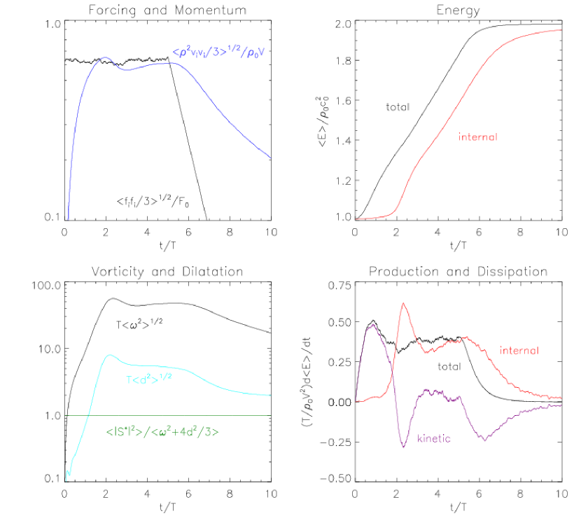
The global statistics of the simulation with $V\approx 0.66c_{0}$, where $c_{0}$ is the initial speed of sound, and $\zeta=3/4$ is shown in figure 1. In this case, the major component of the driving force is solenoidal, but there is a significant dilatational contribution as well. The plot of the RMS velocity shown in the top left panel illustrates the different regimes of the flow evolution. In the beginning, fluid is gradually set into motion. In the course of production, the intensity of turbulence grows exponentially, as one can see from the evolution of the RMS vorticity $\omega=|\nabla\times\vec{v}|$ in the bottom panel on the left. At time $\tilde{t}=t/T\approx 2$, the increase of the kinetic energy stagnates. From $\tilde{t}\approx 3$ onwards, the mean kinetic energy remains roughly constant, and there is an approximate balance between energy injection and dissipation (panels on the right of figure 1). Moreover, the graph of the mean vorticity flattens for $\tilde{t}\gtrsim 2$. Altogether, we take the evolution of the statistical quantities as phenomenological indication of fully developed turbulence at time $\tilde{t}\gtrsim 2$, which asymptotically approaches a statistically homogeneous and stationary state. The conspicuous filaments of intense vorticity, which are the hallmark of developed turbulence, can be seen in a three-dimensional visualisation of the flow at time $\tilde{t}=4.0$ in the figure 7. The intermittency of turbulence becomes manifest in the spacious voids between the vortex filaments. At time $\tilde{t}=\tilde{t}_{\mathrm{d}}=5.0$, the dropping of the random diffusion term in the SDE (7) initiates the exponential decay of the force field, and the energy contents of the flow is subsequently dissipated.

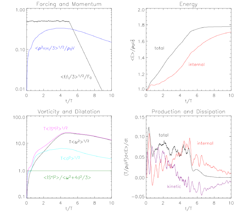
Quite a different behaviour emerges in the case $V/c_{0}=1.39$ and $\zeta=1/5$. As one can see from the plots in figure 2, the rise of the RMS velocity is less steep. Actually, the evolution of the RMS structural invariants $\langle|S^{\ast}|^{2}\rangle^{1/2}$, $\langle\omega^{2}\rangle^{1/2}$ and $\langle d^{2}\rangle^{1/2}$, which is shown in the left bottom panels, suggest that there is an initial phase which is dominated by shocks rather than eddies. This is reflected in pronounced oscillations in the rate of change of kinetic and internal energy, respectively, due to compression and rarefaction effects. At $\tilde{t}\approx 2$, vorticity begins to dominate over the divergence. Apparently, there is a transition from the shock-dominated phase toward a regime, in which the flow becomes increasingly solenoidal, despite of the mostly dilatational force acting upon the fluid. However, since the decay regime was initiated at the time $\tilde{t}=5.0$ too, a statistically stationary flow was not established in this simulation.

Furthermore, we computed a couple of mean structural invariants which correspond to third-order statistical moments of the rate of strain tensor $S_{ij}$. Normalisation with respect to the mean rate of strain $|S|=(2S_{ij}S_{ij})^{1/2}$ gives rise to the definition of the following parameters:

$$a =\frac{\langle\rho|S^{\ast}|^{2}|S|\rangle}{\rho_{0}\langle|S|^{2}\rangle^{3/2}},$$ (13)

$$b =\frac{\langle\rho S_{\!ij}S_{jk}S_{kl}\rangle}{\rho_{0}\langle|S|^{2}\rangle^{3/2}}=\frac{1}{2\sqrt{2}}\mathrm{skew}(S_{\!ik}).$$ (14)

The first parameter, $a$, is closely related to the mean rate of dissipation in the Smagorinsky model. We will comment on this point further in the following section. The parameter $b$, on the other hand, is proportional to the skewness of the rate of strain tensor. Numerical values of $a$ and $b$ evaluated from flow realisations in three simulations at certain instants of time are summarised in table 2. Thereby, a remarkable similarity is revealed. In particular, the rate-of-strain skewness of about $-0.3$ agrees with known results for isotropic turbulence [26]. We take this as a further indication that the flow realisations in our simulations are in good approximation both statistically stationary and isotropic after a few integral time scales have elapsed.

$V/c_{0}$	$t$	$a$	$b$	$\mathrm{skew}(S_{\!ik})$	$\ell_{\mathrm{S}}/\Delta$	$\ell_{\mathrm{S}}/\Delta_{\mathrm{eff}}$
0.084	2.5	1.342	-0.1045	-0.296	0.298	0.17
0.42	3.0	1.339	-0.1041	-0.295	0.260	0.16
0.66	4.0	1.333	-0.1037	-0.293	0.258	0.16

Table 2: Normalised third-order moments of the rate of strain defined in equations (13) and (14) and the equivalent Smagorinsky length in units of $\Delta$ and $\Delta_{\mathrm{eff}}$, respectively.

3 The rate of dissipation

The details of the numerical dissipation produced by the PPM are basically unknown, but it is possible to infer the mean rate of dissipation from the globally averaged energy conservation laws [23]. In fact, there are two distinct mechanisms of dissipation in a compressible fluid. On the one hand, pressure-dilatation accounts for the conversion of internal energy into mechanical energy and vice versa, as fluid, respectively, expands or contracts. Although pressure-dilatation might locally produce mechanical work, it is effectively a dissipative, irreversible process, and the net rate of heat production is given by $-\langle Pd\rangle$, where $d=S_{ii}$ is the divergence of the velocity field. If pronounced shocks are present, however, there might be transient phases in which $\langle Pd\rangle$ becomes positive. This can be seen, for example, in the right bottom panel of figure 2, where the time derivative of the internal energy exhibits local minima corresponding to the production of mechanical energy by pressure-dilatation. On the other hand, the change of internal energy caused by viscous dissipation is strictly negative.

For periodic boundary conditions, the total flux through the boundary surfaces cancels out, and averaging of the internal energy equation thus yields

$$\rho_{0}\epsilon_{\mathrm{num}}=\frac{\mathrm{d}}{\mathrm{d}t}\langle E_{\mathrm{int}}\rangle+\langle Pd\rangle.$$ (15)

Since we do not employ an explicit viscosity term in the equation of motion, $\epsilon_{\mathrm{num}}$ is indeed the mean rate of dissipation due to numerical effects. The corresponding dimensionless dissipation rate $\tilde{\epsilon}_{\mathrm{num}}$ is defined by equation (2). Several representative values of $\tilde{\epsilon}_{\mathrm{num}}$ and the ratio $-\langle Pd\rangle/\epsilon_{\mathrm{num}}$ at certain instants of time are listed in the tables 3, 4 and 5.

In the literature, it is common to normalise the rate of dissipation in terms of the RMS velocity fluctuation $v^{\prime}$ and an integral length scale $\hat{L}$, which is defined by the transversal turbulence energy spectrum $E(k)^{\perp}$:

$$\hat{L}=\frac{\pi}{2v^{\prime\,2}}\int_{0}^{\pi/\Delta}\frac{E(k)^{\perp}\,\mathrm{d}k}{k}\simeq\frac{L}{4v^{\prime\,2}}\sum_{n}\frac{\Phi_{n}^{\perp}}{\tilde{k}_{n}}.$$ (16)

The average kinetic energy $\Phi_{n}^{\perp}$ contained in Fourier modes of wave number $k_{n}$ will be defined in the next section. For isotropic turbulence, $v^{\prime\,2}=\frac{2}{3}\langle e_{\mathrm{kin}}\rangle$, where $e_{\mathrm{kin}}=\frac{1}{2}v^{2}$ is the specific kinetic energy. The parameter $C_{\epsilon}$ specifying the dimensionless rate of dissipation is then given by

$$C_{\epsilon}=\frac{\hat{L}}{v^{\prime\,3}}\langle\epsilon_{\mathrm{num}}\rangle.$$ (17)

Using the instantaneous values of the rate of dissipation and the RMS velocity fluctuations, we estimated $C_{\epsilon}$ for different flow realisations. The accuracy is limited by the calculation of $\hat{L}$, which is mostly determined by the smallest wave numbers, and only few discrete cells are available for $\tilde{k}\sim 1$ in Fourier space. The results are listed in the tables 3, 4 and 5. Generally, $C_{\epsilon}$ is small compared told unity in the production phase. For steady turbulence, values in the range $0.4\ldots 0.5$ are found, which are close to the time-averaged asymptote $\bar{C}_{\epsilon}\approx 0.5$ in simulations of incompressible turbulence [11, 12, 13].

In the introduction, we mentioned that simulations of Eulerian fluids with the PPM, to a certain degree, are equivalent to a LES with explicit modelling of the energy transfer toward unresolved scales in place of numerical dissipation. The consistency of this assumption in terms of statistical quantities can be corroborated for a simple algebraic subgrid scale model such as the Smagorinsky model. The closure for the rate of dissipation in the Smagorinsky model is given by

$$\langle\epsilon_{\mathrm{sgs}}\rangle=a\ell_{\mathrm{S}}^{2}\langle|S|^{2}\rangle^{3/2},\\$$ (18)

where the coefficient $a$ is defined by equation 13, $|S|$ is the rate of strain and $\ell_{\mathrm{S}}$ is a characteristic length of the model. Invoking the condition that $\langle\epsilon_{\mathrm{num}}\rangle$ equals the rate of dissipation predicted by the Smagorinsky model for the given average rate of strain in a particular flow realisation, the Smagorinsky length $\ell_{\mathrm{S}}$ can be calculated. The obtained values in units of $\Delta$ for developed turbulence of three different characteristic Mach numbers are listed in table 2. Moreover, we normalised $\ell_{\mathrm{S}}$ in terms of the effective length scale $\Delta_{\mathrm{eff}}$. The procedure for the calculation of $\Delta_{\mathrm{eff}}$ is introduced in section 5. As we shall argue, $\Delta_{\mathrm{eff}}$ is the appropriate cutoff scale for the PPM. Indeed, the results listed in table 2 verify in each case that $\ell_{\mathrm{S}}/\Delta_{\mathrm{eff}}$ is about $0.16$, which is just the Smagorinsky constant $C_{\mathrm{S}}$ obtained from analytical considerations [25].

$\tilde{t}$	$\langle\tilde{e}_{\mathrm{kin}}\rangle$	$\langle e_{\mathrm{kin}}^{\parallel}\rangle/\langle e_{\mathrm{kin}}\rangle$	$\tilde{\epsilon}_{\mathrm{num}}$	$-\langle Pd\rangle/\rho_{0}\epsilon_{\mathrm{num}}$	$C_{\epsilon}$	$\hat{L}/L$	$l_{\mathrm{p}}/L$	$\beta$
1.5	0.891	$3.74\cdot 10^{-3}$	0.130	0.422	0.077	0.270		1.82
2.0	0.885	$6.74\cdot 10^{-3}$	0.985	0.073	0.51	0.232	0.0659	1.57
3.0	0.728	$8.16\cdot 10^{-3}$	0.474	0.107	0.40	0.281	0.0674	1.62
4.0	0.574	$9.41\cdot 10^{-3}$	0.498	0.053	0.57	0.269	0.0615	1.61
6.0	0.168	$2.13\cdot 10^{-2}$	0.088	0.051	0.83	0.343	0.0644	1.69

Table 3: Mean energy, rate of dissipation and characteristic length scales for a DNS with $V/c_{0}=0.42$ and $\zeta=1.0$.

$\tilde{t}$	$\langle\tilde{e}_{\mathrm{kin}}\rangle$	$\langle e_{\mathrm{kin}}^{\parallel}\rangle/\langle e_{\mathrm{kin}}\rangle$	$\tilde{\epsilon}_{\mathrm{num}}$	$-\langle Pd\rangle/\rho_{0}\epsilon_{\mathrm{num}}$	$C_{\epsilon}$	$\hat{L}/L$	$l_{\mathrm{p}}/L$	$\beta$
2.0	0.668	$2.25\cdot 10^{-2}$	0.322	0.158	0.26	0.229	0.0830	1.66
4.0	0.544	$2.10\cdot 10^{-2}$	0.305	0.106	0.40	0.279	0.0601	1.62
5.0	0.571	$1.87\cdot 10^{-2}$	0.350	0.070	0.44	0.285	0.0659	1.61
7.0	0.252	$2.75\cdot 10^{-2}$	0.170	0.059	0.74	0.286	0.0601	1.61
9.0	0.092	$6.72\cdot 10^{-2}$	0.037	-0.150	0.86	0.318	0.0644	1.69

Table 4: Mean energy, rate of dissipation and characteristic length scales for a DNS with $V/c_{0}=0.66$ and $\zeta=0.75$.

$\tilde{t}$	$\langle\tilde{e}_{\mathrm{kin}}\rangle$	$\langle e_{\mathrm{kin}}^{\parallel}\rangle/\langle e_{\mathrm{kin}}\rangle$	$\tilde{\epsilon}_{\mathrm{num}}$	$-\langle Pd\rangle/\rho_{0}\epsilon_{\mathrm{num}}$	$C_{\epsilon}$	$\hat{L}/L$	$l_{\mathrm{p}}/L$	$\beta$
2.0	0.103	0.250	0.0105	0.663	0.30	0.332	0.323	5.57
3.5	0.157	0.195	0.0278	0.940	0.30	0.260	0.229	2.24
5.0	0.147	0.189	0.0618	0.147	0.66	0.241	0.066	1.75
6.0	0.121	0.134	0.0443	0.198	0.60	0.251	0.063	1.71
9.0	0.045	0.158	0.0141	-0.078	0.93	0.265	0.060	1.68

Table 5: Mean energy, rate of dissipation and characteristic length scales for a DNS with $V/c_{0}=1.39$ and $\zeta=0.2$.

4 Turbulence energy spectra

In the case of isotropic turbulence, the sum over all squared Fourier modes of the velocity field can be expressed as an integral over a function of the wave number only:

$$\frac{1}{V^{2}}\sum_{jlm}\frac{1}{2}\langle\hat{\vec{v}}_{jlm}(t)\cdot\hat{\vec{v}}_{jlm}^{\,\ast}(t)\rangle=\int_{0}^{\infty}\mathrm{d}(\alpha\tilde{k})\tilde{E}(\alpha\tilde{k},t)$$ (19)

Here the wave number is written in dimensionless form as $\tilde{k}=Lk/2\pi$. The function $E(k,t)=(\alpha L/2\pi)V^{2}\tilde{E}(\alpha\tilde{k},t)$ is called the energy spectrum function. For a discrete spectrum of modes, $\tilde{E}(\alpha\tilde{k},t)$ is a generalised function which is defined by:

$$\tilde{E}(\alpha\tilde{k},t)=\frac{1}{V^{2}}\sum_{jlm}\frac{1}{2}\langle\hat{\vec{v}}_{jlm}(t)\cdot\hat{\vec{v}}_{jlm}^{\,\ast}(t)\rangle\delta[\alpha\tilde{k}-(j^{2}+l^{2}+m^{2})^{1/2}].$$ (20)

For the numerical evaluation, we define an approximation to $\tilde{E}(\alpha\tilde{k},t)$ by summing over wave number bins $[k_{n-1/2},k_{n+1/2}]$. This yields the discrete set of numbers

$$\tilde{E}_{n}(t)=\frac{4\pi(\alpha\tilde{k}_{n})^{2}}{V^{2}}\Phi_{n}(t),$$ (21)

where $k_{n}=\frac{1}{2}(k_{n-1/2}+k_{n+1/2})$, and $\Phi_{n}(t)$ is the average kinetic energy of all modes in the corresponding wave number bin:

$$\Phi_{n}(t)=\frac{1}{\tilde{\mu}_{n}}\sum_{\alpha^{2}\tilde{k}_{n-1/2}^{2}\leq\alpha^{2}\tilde{k}^{2}\leq\alpha^{2}\tilde{k}_{n+1/2}^{2}}\sum_{jlm}\frac{1}{2}\hat{\vec{v}}_{jlm}(t)\cdot\hat{\vec{v}}_{jlm}^{\,\ast}(t)\delta_{j^{2}+l^{2}+m^{2}}^{\alpha^{2}\tilde{k}^{2}}.$$ (22)

Here $\tilde{\mu_{n}}$ is the statistical weight of the $n$th wave number bin, i. e., the number of cells in Fourier space with wavenumber $k_{jlm}\in[k_{n-1/2},k_{n+1/2}]$.

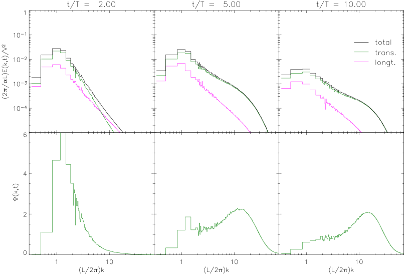
A number of spectra were computed from flow realisations at selected times. Some of these spectra are shown in Figures 3, 4 and 5. For the calculation of the discrete spectrum function as given by definition (21), a coarse equidistant wave number mesh was used in the energy containing range, $0\leq\tilde{k}\leq 2$, and a logarithmic mesh with narrow bins for the larger wave numbers. The panels on the top of figure 3 show, from left to right, the discrete energy spectrum function $\tilde{E}_{n}(t)$ at representative stages for the simulation with $\zeta=1.0$ and characteristic Mach number $V/c_{0}\approx 0.42$. The panel on the very left shows a spectrum in the production phase. The middle panel corresponds to developed turbulence, and the panel on the very right shows a spectrum for decaying turbulence. One can clearly see the larger energy contents at high wave numbers in the case of developed turbulence and the lower overall energy budget in the decay regime. Also plotted are the longitudinal and transversal spectrum functions, $\tilde{E}_{n}^{\parallel}(t)$ and $\tilde{E}_{n}^{\perp}(t)$, respectively. $\tilde{E}_{n}^{\parallel}(t)$ corresponds to the dilatational (rotation-free) components of the flow and $\tilde{E}_{n}^{\perp}(t)$ to the solenoidal (divergence-free) components. From the plots in figure 3, it becomes apparent that the longitudinal energy fraction at higher wave numbers decays faster in comparison to the transversal fraction. The energy in the longitudinal components at small wave numbers, on the other hand, remains almost constant.

Figure 3: Turbulence energy spectrum functions for $V/c_{0}=0.42$ and $\zeta=1.0$. In the bottom panels, the compensated spectrum functions corresponding to the transversal component are plotted.

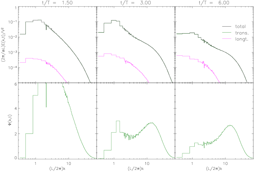
From the Kolmogorov spectrum function (1), it follows that $\langle\epsilon\rangle^{-2/3}k^{5/3}E^{\perp}(k)$ is approximately constant in the inertial subrange of wave numbers. This suggests the definition of a compensated spectrum function,

$$\Psi_{n}^{\perp}(t)=\left[\frac{\alpha}{2\pi}\langle\tilde{\epsilon}(t)\rangle\right]^{-2/3}(\alpha\tilde{k}_{n})^{5/3}\tilde{E}_{n}^{\perp}(t),$$ (23)

as an indicator of Kolmogorov scaling. Note that only the transversal part of the energy spectrum is compensated, because it is the incompressible fraction of turbulence energy which a priori fulfils Kolmogorov scaling. For the calculation of $\Psi_{n}^{\perp}(t)$, the values of $\langle{\tilde{\epsilon}}_{\mathrm{num}}\rangle$ listed in the tables 3, 4 and 5 were substituted for the dimensionless mean rate of dissipation in equation (23). The resulting plots of the compensated spectrum functions for $\zeta=1.0$ are shown in the bottom panels of figure 3. In particular, the graph of $\tilde{\Psi}_{n}^{\perp}(t)$ for $t=3.0$ verifies the existence of a narrow window of wave numbers in the vicinity of $\tilde{k}=3.0$, in which Kolmogorov scaling with $C\approx 1.7$ applies within the bounds set by the numerical uncertainty. It is noteworthy that this value is very close to results obtained from other numerical simulations, especially, those with higher resolution [4, 10, 11]. However, the Kolmogorov constant inferred from our simulations might be systematically too large, because of the lack of isotropy for wave numbers close to the energy-containing subrange [4]. Moreover, the portion of the compensated spectrum function $\tilde{\Psi}_{n}^{\perp}(t=3T)$ in the range of dimensionless wave numbers between $2$ and about $4$ appears to be consistent with a modification of the Kolmogorov exponent by $-0.1$ , which has recently been inferred from a DNS with extremely high resolution [11].

Figure 4: Turbulence energy spectra for $V/c_{0}=0.66$ and $\zeta=0.75$.

Figure 5: Turbulence energy spectra for $V/c_{0}=1.39$ and $\zeta=0.2$.

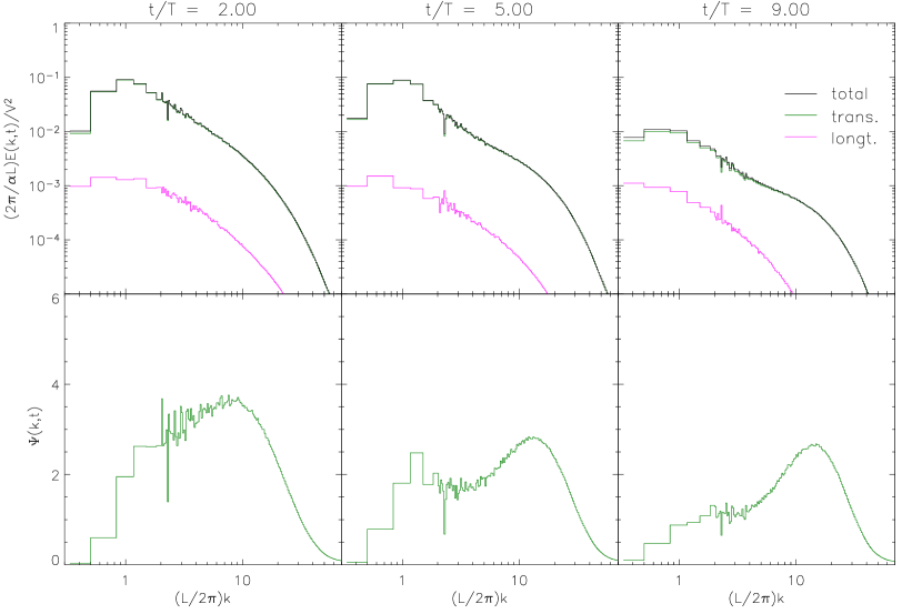
Basically the same results hold for the simulation with higher characteristic Mach number, $V/c_{0}\approx 0.66$, and $\zeta=0.75$. The sample spectra shown in figure 4 are very similar in shape compared to those in figure 3, except for the smaller gap between the total and the longitudinal energy spectrum functions. As for the case $\zeta=0.2$ and $V/c_{0}\approx 1.39$, differences can evidently be seen in figure 5. At early time, the flow is dominated by large shock waves and most of the energy is contained in longitudinal modes. This is illustrated by the plot of the energy spectrum functions at time $\tilde{t}=2.0$. The scaling deviates markedly from the Kolmogorov law. In particular, the longitudinal component $E_{n}^{\parallel}(t)$ clearly obeys a power law with exponent $-2$ and the transversal component is falling off even steeper. From statistics of the velocity field shown in figure 2, a transition to the regime of solenoidal turbulent flow around $\tilde{t}\approx 3.0$ can be discerned [6]. In this regime, the small-scale dynamics is eventually dominated by turbulent vortices as in the case of subsonic turbulence, and the transversal component of the energy spectrum function is more or less Kolmogorovian. However, we have a somewhat smaller value of the Kolmogorov constant, $C\approx 1.3$, at time $\tilde{t}=5.0$ (see the middle panels in figure 5).

For developed turbulence, there is a pronounced maximum of the compensated spectrum function at $\tilde{k}\approx 15$ corresponding to a flattening of the energy spectrum in comparison to the Kolmogorov law. This so-called bottleneck effect has actually been observed in various numerical simulations [3, 9, 14, 15]. The anomalous bottleneck scaling is attributed to dynamical peculiarities on scales which are significantly influenced by dissipation. For example, experimental data indicate a $k^{-1}$ power law behaviour of the energy spectrum function in the vicinity of the wave number of maximum dissipation [2]. A theoretical explanation of the bottleneck effect on grounds of the non-linear turbulent transfer was suggested too [17]. The peak of $\tilde{\Psi}_{n}(t)$ close to the wave number $\tilde{k}\approx 15$ is more pronounced than in simulations of incompressible turbulence with spectral methods. For instance, the peak value in the middle panels of the figures 3 and 4 is about $2.9$, whereas the peaks of the compensated spectra in [3, 11] are not much higher than $2.0$. The width of the bottleneck, on the other hand, is about one decade in wave number space in all cases. Remarkably, the properties of the bottleneck we observe are very similar to what is found in turbulence simulations with hyperviscosity [15]. Thus, it appears that the numerical viscosity of the PPM acts like a hyperviscosity, at least as far as the spectral distribution of turbulence energy is concerned.

5 Dissipation length scales

One can regard the action of numerical dissipation as being equivalent to an implicit filter smoothing the flow on a certain length scale, say, $\Delta_{\mathrm{eff}}$. Fourier modes of wave number larger than $\pi/\Delta_{\mathrm{eff}}$ are suppressed. It has already been pointed out in section 3 that the ratio $\beta=\Delta_{\mathrm{eff}}/\Delta$ is of particular interest for subgrid scale models, which depend on the reliable specification of the cutoff length. In combination with a finite-volume method, the cutoff length may very well be different form the grid resolution $\Delta$. Although the common point of view holds that it is not sensible to apply a subgrid scale model in combination with dissipative schemes such as the PPM, subgrid scale models are used in some applications without active coupling to the resolved flow. A particular example is the modelling of turbulent combustion, where the subgrid scale energy is treated as a passive scalar and is used as input for a turbulent flame speed model [19, 20, 21].

The determination of the effective length scale $\Delta_{\mathrm{eff}}$ for the PPM makes use of the notion of a characteristic filter scale [29]. For a one-dimensional filter of explicitly known functional form, the characteristic length can be calculated from the second moment of the Fourier transform of the filter kernel, the so-called transfer function. However, since the implicit filter associated with the PPM is not explicitly known, we have to resort to the numerically computed energy spectra. Using Kolmogorov’s law as reference spectrum function, we define an effective transfer function

$$\hat{G}_{\mathrm{eff}}^{2}(k,t)=\frac{E(k,t)}{E_{\infty}(k,t)}=\frac{1}{C}\Psi(k,t),$$ (24)

where $E_{\infty}(k,t)=C\epsilon_{\mathrm{num}}^{2/3}(t)k^{-5/3}$. The second moment of the squared transfer function is given by

$$M^{(2)}[\hat{G}_{\mathrm{eff}}^{2}]=\int_{0}^{\infty}k^{2}\hat{G}_{\mathrm{eff}}^{2}(k,t)\mathrm{d}k.$$ (25)

Of course, the numerically computed spectrum function $E(k,t)$ does not conform with the Kolmogorov law at wave numbers comparable to $k_{0}=2\pi/L$, because of energy injection on the largest length scales. However, the contribution of these wave numbers to the above integral is small due to the factor $k^{2}$. Thus, we will ignore this error.

Discretising the transfer function in the fashion outlined in section 4 and cutting off at the wavelength $\pi/\Delta$, the following approximation to the second moment is obtained:

$$M^{(2)}[\hat{G}_{\mathrm{eff}}^{2}]\simeq\frac{1}{C}\left(\frac{2\pi}{\alpha L}\right)^{3}\int_{0}^{N/2}\mathrm{d}(\alpha\tilde{k})\sum_{n}\Psi_{n}(t)\frac{\tilde{\mu}_{n}}{4\pi}\delta[\alpha(\tilde{k}-\tilde{k}_{n})].$$ (26)

The second moment of the filter transfer function has the dimension of inverse length cubed. Hence, a length scale is given by $(M^{(2)}[\hat{G^{2}}])^{-1/3}$ and is customarily normalised with respect to the second moment of the sharp cutoff filter. The transfer function of this filter is given by $\hat{G}_{\Delta}(k)=\theta(\pi/\Delta-k)$, and the second moment is $M^{(2)}[\hat{G}_{\Delta}^{2}]=(\pi/\Delta)^{3}/3$. Setting $M^{(2)}[\hat{G}_{\mathrm{eff}}^{2}]=(\pi/\Delta_{\mathrm{eff}})^{3}/3$, the effective filter scaling factor of the PPM is therefore estimated to be

$$\beta=\frac{\Delta_{\mathrm{eff}}}{\Delta}=\frac{N}{2}\left[\frac{3}{C}\sum_{n=1}^{n_{\mathrm{c}}}\Psi_{n}(t)\frac{\tilde{\mu}_{n}}{4\pi}\right]^{-1/3},$$ (27)

where $n_{\mathrm{c}}=\max\{n|\tilde{k}_{n}\leq\tilde{k}_{\mathrm{c}}\}$.

We calculated $\beta$ for each simulation at several instants of time. The obtained values listed in the tables 3, 4 and 5 demonstrate that $\Delta_{\mathrm{eff}}\approx 1.6\Delta$ for fully developed turbulence. Only for the lowest Mach number, $V/c_{0}\approx 0.084$, the scaling factor $\beta\approx 1.8$ was found in the stationary regime. Consequently, the effect of numerical dissipation appears to become more pronounced for decreasing Mach number. Of course, the dependence of $\beta$ on the numerical resolution should be investigated too. Changes can be expected towards lower resolution, because the energy-containing and the dissipation subrange will increasingly overlap. At higher resolution, on the other hand, $\beta$ should asymptotically approach a value independent of $N$. Unfortunately, the validation of this conjecture would require an undue amount of computational resources.

In fact, $\Delta_{\mathrm{eff}}$ is much smaller than the length scale of maximum dissipation, $l_{\mathrm{p}}$, which is given by the maximum of $\tilde{k}_{n}^{2}\tilde{E}_{n}(t)\propto\tilde{k}_{n}^{1/3}\tilde{\Psi}_{n}(t)$. For fully developed turbulence, the peak of dissipation was found to be located close to the second maximum of $\tilde{\Psi}_{n}(t)$, with a typical value $l_{\mathrm{p}}\approx 0.065L\approx 9\Delta$ (see tables 3, 4 and 5). Thus, $l_{\mathrm{p}}$ can be considered as the characteristic length scale of the bottleneck effect. The morphology of the flow on length scales $l\gtrsim l_{\mathrm{p}}$ is illustrated in figure 6. Shown are the isosurfaces of vorticity which correspond to the $97\,\%$ level of the probability distribution function. In order to suppress velocity fluctuations on scales smaller than $l_{\mathrm{p}}$, a Gaussian filter of characteristic length $10\Delta_{\mathrm{eff}}\approx 2l_{\mathrm{p}}$ was applied to the flow realisation at time $\tilde{t}=4.0$. The characteristic Mach number is $V/c_{0}=0.66$ and the spectral weight $\zeta=3/4$. The smoothing of the velocity field over a length $2\Delta_{\mathrm{eff}}\approx l_{\mathrm{p}}/3$ results in the visualisation shown in figure 7. Although the length scales smaller than $l_{\mathrm{p}}$ are subject to significant numerical dissipation, there is nevertheless a great wealth of substructure on these scales. It becomes clear that the tube-like structures in figure 6 are actually concentrations of smaller vortices. The magnitude of the flow velocity is colour-coded in the plots. It appears that a significant fraction of high velocity fluctuations is present on the length scales $l\lesssim l_{\mathrm{p}}$ in the bottleneck subrange of the turbulence energy spectrum.

This figure is not available in the e-print version.

Figure 6: Isosurfaces of vorticity for the same flow realisation as in figure 6, however, with the velocity field smoothed on the length scale $10\Delta_{\mathrm{eff}}=16.2\Delta$, which is about the length scale of peak dissipation.

This figure is not available in the e-print version.

Figure 7: Isosurfaces of vorticity for developed turbulence in the simulation with $V/c_{0}=0.66$ and $\zeta=0.75$. The velocity field was smoothed with a Gaussian filter of characteristic length $2\Delta_{\mathrm{eff}}=3.24\Delta$. The colour coding corresponds to the dimensionless velocity $v/V$.

6 Conclusion

The computation of turbulence energy spectrum functions reveals several important properties of turbulence in numerical simulations with the PPM: Firstly, the range of length scales approximately satisfying Kolmogorov scaling, secondly, characteristic scales associated with numerical dissipation, and thirdly, the so-called bottleneck effect, i. e., an excess of kinetic energy in modes affected by dissipation.

For the simulations of forced isotropic turbulence discussed in this paper, there is only a marginal inertial subrange. Nevertheless, we were able to estimate the Kolmogorov constant for samples of the flow in the nearly statistically stationary regime to be $C\approx 1.7$, which agrees very well with published results from more elaborate simulations. Only in the case of a simulation with Mach number of order unity and forcing dominated by dilatational components, a significantly smaller value of $C$ was found. On the basis of the notion of an implicit filter, we define the length scale $\Delta_{\mathrm{eff}}$ specifying the characteristic length of smoothing due to the numerical scheme. The ratio $\beta=\Delta_{\mathrm{eff}}/\Delta$ appears to be fairly universal for statistically stationary turbulence. In the case of the PPM, $\beta\approx 1.6$. Furthermore, it was demonstrated that the computed spectra exhibit a pronounced bottleneck effect. The corresponding peak is higher than in spectra obtained from simulations with spectral methods. The magnitude of the bottleneck effect appears to be similar to what is obtained in simulations with hyperviscosity.

The parameter $C_{\epsilon}$ specifying the dimensionless rate of numerical dissipation assumes values of about $0.5$ for developed turbulence. This is consistent with the time-averaged asymptotic value in the limit of large Reynolds numbers calculated from simulations of incompressible turbulence. From the mean rate of numerical dissipation, one can also compute an equivalent Smagorinsky length. The ratio of this length to $\Delta_{\mathrm{eff}}$ is very close to the analytical value of the Smagorinsky constant $C_{\mathrm{S}}$. This result supports the presumed statistical equivalence of numerical dissipation in simulations with the PPM and the subgrid scale energy transfer in proper LES.

In essence, the presented results suggest that the application of the PPM in fluid dynamical simulations yields a fair numerical representation of turbulent flows, for which crucial statistical parameters are in good agreement with the results obtained with more accurate methods.

7 Acknowledgements

The turbulence simulations were run on the Hitachi SR-8000 of the Leibniz Computing Centre in Munich, and the post-processing of the data was performed on the IBM p690 of the Computing Centre of the Max-Planck-Society in Garching, Germany. We thank M. Reinecke, who was very helpful with technical advice. For the computation of the turbulence energy spectra, the FFTW implementation of the the fast Fourier transform algorithm was utilised [30]. The research of W. Schmidt was in part supported by the priority research program Analysis and Numerics for Conservation Laws of the Deutsche Forschungsgesellschaft. Moreover, W. Schmidt and J. C. Niemeyer were supported by the Alfried Krupp Prize for Young University Teachers of the Alfried Krupp von Bohlen und Halbach Foundation.

References

- [1] Kolmogorov, A. N.: C. R. Acad. Sci. URSS 30, 301 (1941)
- [2] She, Z., Jackson, E.: On the universal form of energy spectra in fully developed turbulence, Phys. Fluids A 5 (7), , 1526–1528 (1993)
- [3] Cao, N., Chen, S., She, Z.: Scalings and Relative Scalings in the Navier-Stokes Turbulence, Phys. Rev. Letters 76, 3711–3714 (1996)
- [4] Yeung, P. K., Zhou, Y.: Universality of the Kolmogorov constant in numerical simulations of turbulence, Phys. Rev. E 56, 1746–1752 (1997)
- [5] Colella, P., Woodward, P. R.: The piecewise parabolic method (PPM) for gas-dynamical simulations, J. Comp. Phys. 54, 174–201 (1984)
- [6] Porter, D. H., Pouquet, A., Woodward, P. R.: Three-dimensional supersonic homogeneous turbulence - A numerical study, Phys. Rev. Letters 68, 3156–3159 (1992)
- [7] Porter, D. H., Pouquet, A., Woodward, P. R.: Kolmogorov-like spectra in decaying three-dimensional supersonic flows, Phys. Fluids 6 (6), 2133–2142 (1994)
- [8] Porter, D. H., Woodward, P. R., Pouquet, A.: Inertial range structures in decaying compressible turbulent flows, Phys. Fluids 10 (1), 237–245 (1998)
- [9] Sytine, I. V., Porter, D. H., Woodward, P. R., Hodson, S. W., Winkler, K.: Convergence Tests for the Piecewise Parabolic Method and Navier-Stokes Solutions for Homogeneous Compressible Turbulence, J. Comp. Phys. 158, 225–238 (2000)
- [10] Goto, T., and Fukayama, D.: Pressure Spectrum in Homogeneous Turbulence, Phys. Rev. Letters 86, 3775–3778 (2001)
- [11] Kaneda, Y., Ishihara, T., Yokokawa, M., Itakura, K., Uno, A.: Energy dissipation rate and energy spectrum in high resolution direct numerical simulations of turbulence in a periodic box”, Phys. Fluids 15, L21–L24 (2003)
- [12] Sreenivasan, K. R.: An update on the energy dissipation rate in isotropic turbulence, Phys. Fluids 10, 528–529 (1998)
- [13] Pearson, B. R., Krogstad, P.-Å., van de Water, W.: Measurements of the turbulent energy dissipation rate, Phys. Fluids 14, 1288–1290 (2002)
- [14] Dobler, W., Haugen, N. E., Yousef, T. A., Brandenburg, A.: Bottleneck effect in three-dimensional turbulence simulations, Phys. Rev. E 68, 026304 (2003)
- [15] Haugen, N. E. L., Brandenburg, A.: Inertial range scaling in numerical turbulence with hyperviscosity, Phys. Rev. E, 70, 026405 (2004)
- [16] Pearson, B. W., Yousef, T. A., Haugen, N. E., Brandenburg, A., Krogstad, P.-Å.: The ”zeroth law” of turbulence: Isotropic turbulence simulations revisited, submitted to Phys. Rev. E, preprint physics/0404114 (2004)
- [17] Falkovich, G.: Bottleneck phenomenon in developed turbulence, Phys. Fluids 6, 1411–1414 (1994)
- [18] Rider, W. J., Drikakis, D.: High Resolution Methods for Computing Turbulent Flows in Turbulent Flow Computation, Kluwer Acad. Publ. (2002)
- [19] Niemeyer, J. C., Hillebrandt, W.: Turbulent Nuclear Flames in Type Ia Supernovae, Astrophys. J. 452, 769–778 (1995)
- [20] Hillebrandt, W., Niemeyer, J. C.: Type Ia supernova explosion models, Ann. Rev. Astron. Astrophys. 38, 191 (2000)
-
[21]
Schmidt, W., Turbulent Thermonuclear
Combustion in Degenerate Stars, PhD Thesis, Technical University of
Munich,
http://tumb1.biblio.tu-muenchen.de/publ/diss/ph/2004/schmidt.html (2004) - [22] Landau, L. D., Lifshitz, E. M.: Fluid mechanics, Pergamon Press (1987)
- [23] Warsi, Z. U. A.: Fluid Dynamics: Theoretical and Computational Approaches, CRC Press (1993)
- [24] Eswaran, V., Pope, S. B.: An examination of forcing in direct numerical simulations of turbulence, Comput. Fluids 16 (3), 257–278 (1988)
- [25] Pope, S. B.: Turbulent Flows, Cambridge University Press (2000)
- [26] Kosović, B.: Subgrid-scale modelling for the large-eddy simulation of high-Reynolds-number boundary layers, J. Fluid Mech. 336, 151–182 (1997)
- [27] Shapiro, S. L., Teukolsky, S. A.: Black Holes, White Dwarfs and Neutron Stars, John Wiley & Sons (1983)
[28]
Reinecke, M.: Modeling and simulation of
turbulent combustion in type Ia supernovae, PhD Thesis, Technical
University of Munich,
http://tumb1.biblio.tu-muenchen.de/publ/diss/ph/2001/reinecke.html (2001) - [29] Lund, T. S.: On the use of discrete filters for large eddy simulation, Annual Research Briefs, Center for Turbulence Research, Stanford, 83–96 (1997)
- [30] Frigo, M., Johnson, S. G.: FFTW: An Adaptive Software Architecture for the FFT, ICASSP conference proceedings 3, 1381–1384 (1998)