The radial extinction profiles of late-type galaxies

We have used UV (FOCA) and FIR (IRAS) images of six nearby late type galaxies to study the radial variation of the UV extinction (deduced from the FIR/UV ratio). We compare the UV extinction gradient with other extinction indicators (Balmer decrement) and search for a relation between the extinction, the metallicity and the gas surface density among our galaxies. We detect in our small sample a clear relation between extinction and metallicity. These observed relations are used to calibrate an empirical recipe useful for extinction correction in the UV, visible and near-infrared images of late type galaxies.

1 Introduction

The physical properties of late type galaxies, and in particular the ones that are determined from the stellar emission can be studied only after an accurate dust extinction correction. It is thus crucial to have a sound understanding of the dust extinction in late type galaxies before studying nearby as well as high redshift galaxies (especially since the latter are observed in the optical in UV-rest frame, where the extinction is particularly severe).

The definition of an accurate model useful for correcting the UV, optical and near infra-red data for the dust extinction in disc galaxies is particularly difficult because of several uncertainties: i) little is known about the relative geometrical distribution of the dust and stars of various spectral types and ages at small and large scales. On small scales, young stars spend a finite time within the star forming regions before migrating out of them (e.g. Charlot & Fall 2000; Panuzzo et al. 2003). On large scales, the properties and distributions of HII regions in spiral discs vary with the morphological type (Kennicutt et al. 1989). ii) the extinction law (variation of the extinction with wavelength) presents large variations for different lines of sight in the Galaxy, and different shapes in the Galaxy and in the Magellanic Clouds, in particular in the UV domain (e.g. Savage & Mathis 1979). It is thus unclear which extinction law should be applied. iii) Despite recent significant improvement in characterising the extinction curve (e.g. Desert et al. 1990), the nature of the dust (composition, size distribution) is still poorly known.

There are however several observational ways to directly estimate the dust extinction in well defined spectral ranges: using the Balmer lines by comparing the observed to the expected decrement (Lequeux et al. 1981; McCall et al. 1985; Kennicutt 1992), and in the UV from the FIR (Far Infra Red) to UV ratio (e.g. Buat & Xu 1996; Calzetti et al. 2000; Panuzzo et al. 2003; Charlot & Fall 2000; Boselli et al. 2003),or from the slope $\beta$ of the UV continuum (e.g. Calzetti et al. 1994; Meurer et al. 1995, 1999; Bell 2002).

The Balmer decrement gives a good measure of the differential extinction between the lines outside of the ionized region. Its use however requires an accurate determination of the underlying Balmer absorption. Ideally, one needs high quality spectra and good resolution for this purpose. In resolved galaxies, this method can only be applied to HII regions. Given their peculiar nature, the effects of age and geometrical distribution (e.g. Charlot & Fall 2000; Poggianti et al. 2001; Panuzzo et al. 2003) make it difficult to extrapolate the results to the galaxy as a whole or to other wavelengths. Calzetti et al. (1994) proposed a relation to link the Balmer decrement to the extinction in the UV and optical in starbursts, which was subsequently found not to be valid in normal galaxies (Bell 2002; Buat et al. 2002).

Various models (Witt & Gordon 2000; Panuzzo et al. 2003) have shown that the FIR/UV ratio is the most reliable measure of the UV attenuation, depending weakly on the relative geometry of the stars and the dust, the extinction law, or the nature of the underlying stellar population. This results from the fact that the stellar population heating the dust (emitting in the far infra-red) is the same population responsible for the UV emission.

Buat & Xu (1996) used a radiative transfer model to derive the extinction of 152 disk galaxies observed both in the UV and in the infrared, using the FIR/UV ratio. They found relatively moderate extinctions (0.9 and 0.2 magnitude for early-type and late-type disk galaxies respectively). It has also been used by Boselli et al. (2003) in a large sample of 118 Virgo galaxies. They found an average UV extinction of 1.28, 0.85, 0.68 for galaxies of type Sa-Sbc, Sc-Scd, Sd-Im-BCD respectively. In association with a geometrical model, the FIR/UV ratio can be used to predict the dust extinction at all wavelengths, as was done in a simplistic way by Boselli et al. (2003).

While the FIR/UV ratio has been used successfully in unresolved galaxies, it has never been studied in spatially resolved objects. While many profiles are available for nearby galaxies (surface brightness at various wavelengths, gas, metallicity), we do not know generally the radial distribution of extinction in normal late-type spirals.

We propose in this paper to adopt the FIR/UV as an extinction diagnostic for spatially resolved nearby galaxies. This is done by computing FIR and UV radial profiles, and deducing from them reliable extinction profiles. The FIR/UV ratio does not trace extinction on small scales (because of geometrical and transfer effects) but this problem is avoided by considering azimuthally averaged profiles and working at relatively low resolution. This radial variation of the dust attenuation will be compared to the frequently used Balmer decrement gradient.

Our next goal will be to give to the reader an empirical recipe for correcting for extinction UV to near-infrared radial profiles (at least in a statistical sense). This will be achieved by studying the dependence of the dust extinction on other local properties that are likely to affect the amount of dust: the metallicity and the gas surface density.

The data used are presented in Sect. 2: FOCA UV images of 6 nearby galaxies with their IRAS FIR counter-part. We also present the gaseous profiles and HII region (abundances and extinctions) data used in our investigation. While our input data (UV and FIR fluxes, metallicity, gas surface density) tend to decrease with the radius, it is still unknown what is the radial variation of the dust extinction (as traced by the FIR/UV ratio) and of the dust to gas ratio. In Sect. 3, we present the extinction profiles obtained in the UV, and predicted at other wavelengths with the help of a simple model. In Sect. 4, we compare the attenuation in the UV with the one derived from Hydrogen lines in HII regions. In Sect. 5, we study the dependence of the extinction and the dust-to-gas ratio on the metallicity. We propose a simple prescription to estimate the extinction profile in any galaxy with either a known abundance gradient, or a blue absolute magnitude and scale-length. Our most important results are summarised in Sect. 6.

2 Data and methodology

The first purpose of this work is to obtain reliable dust extinction gradients from the FIR/UV ratio of resolved galaxies. This exercise is however strongly limited by the lack of UV images of FIR IRAS resolved galaxies, and by the poor FIR spatial resolution of the IRAS images. Indeed the sample of galaxies large enough to be spatially resolved at 100 $\mu$m is quite small (Rice 1993).

At the present time, only six galaxies satisfy these conditions. In the UV, the images we will use were obtained by FOCA at 2000 Å (FOCA is described in Milliard et al. 1991). Their characteristics are given in Table 1. IRAS images at 60 and 100 $\mu$m are available for 5 of them in the high resolution catalogue of Rice (1993). For the last one (M100), we made an IRAS HIRES request to the IPAC web page. General properties and the integrated fluxes of the sample galaxies are given in Table 2.

Table 1: UV characteristics of the FOCA images.

Galaxy	Resolution	Exposure
	arcsec	sec
(1)	(2)	(3)
M33	20	9 x 150
M51	12	4 x 300
M81	12	11 x 150
M100	12	4 x 200
M101	12	4 x 300
M106	20	4 x 150

Table 2: Properties of the target galaxies.

Galaxy	UV	H	60 $\mu$m	100 $\mu$m	$D$	$Type$	$D_{25}$	$B_{T}$	$12+log(O/H)$
	mag	mag	Jy	Jy	Mpc		arcmin	mag	at center
(1)	(2)	(3)	(4)	(5)	(6)	(7)	(8)	(9)	(10)
M33	6.12	4.35	421.6	1102.3	0.70	SAcd	70.8	6.27	9.08
M51	8.88	5.65	106.1	266.8	8.40	SAbc	11.2	8.96	9.38
M81	8.97	4.09	42.7	161.9	3.63	SAab	26.9	7.89	9.35
M100	10.56	6.81	25.9	69.2	17.00	SABbc	7.4	10.05	9.36
M101	7.99	5.80	72.1	200.8	7.48	SABcd	28.8	8.31	9.06
M106	10.02	5.71	26.4	77.8	7.98	SABbc	18.6	9.10	9.09

Column 1: Galaxy name. Column 2: the UV magnitude from FOCA images integrated within the largest radius used for this analysis. The FOCA magnitude is defined as $m_{UV}$=-2.5 log($F$)-21.175, where $F$ is the flux in erg cm^-2 s^-1 A^-1). Column 3: H band magnitude (Jarrett et al. 2003). Column 4 and 5 : Flux densities (IRAS) at 60 and 100 $\mu$m in Jy (Rice 1993). Column 6 : Distance in Mpc. References: Madore et al. (1985), Feldmeier et al. (1997), Freedman et al. (2001), Ferrarese et al. (2000). 17 Mpc is adopted for M100, as a member of Virgo. Column 7 : Morphological type (as found in NED). Column 8 : Major axis diameter at the 25.0 mag arcsec^-2 isophote in B, Column 9 : total B magnitude (columns 8 and 9 are taken from the RC3 catalogue). Column 10: Central abundance (deduced from the abundance gradient extrapolated to radius=0).

These 6 galaxies do not constitute a complete sample in any sense, but are the few nearby objects for which a resolved analysis of the ratio FIR(IRAS)/UV(FOCA) is possible at the present time.

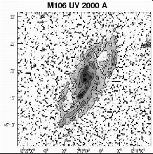
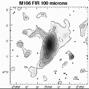
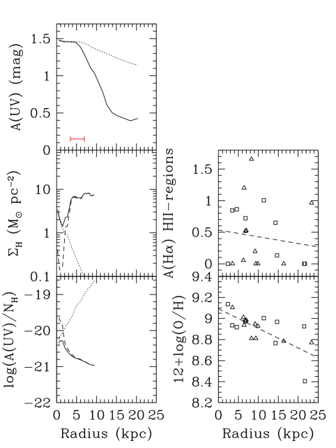
Figure 6: Profiles in M106. Same caption as for Fig. 1.

The determination of the radial variation of the FIR to UV flux ratio is done after computing the independent FIR (60 and 100 $\mu$m and UV radial profiles (see Sect. 2.4). The images of each galaxy in the UV and at 100 $\mu$m are shown in Figs. 1 to 6 (respectively in the top-right and bottom-right panels). The calculation of the extinction profiles (the UV extinction profile is shown in the top-left panel of Figs. 1-6) is reported in Sect. 3.

Once an extinction gradient has been obtained from the FIR/UV ratio, our next goals are (a) to compare them with other extinction indicators (b) to see whether the extinction within galaxies is related to other entities like the gas density or the metallicity. If present, these relationships would be extremely useful for a more accurate computation of the effects of dust in galaxy evolution models in which extinction is often simply estimated from gas densities and abundances (e.g. Guiderdoni & Rocca-Volmerange, 1987).

HII regions can provide us with additional information since their spectroscopic observation can be used to have an independent dust extinction estimate (through the Balmer decrement) and for the determination of the metallicity gradient. Data in HII regions have thus been collected for each galaxy. They are presented in the middle column of Figs. 1-6 and discussed in Sect.s 2.1 (extinction) and 2.2 (abundances).

We finally need gas profiles. They are presented in the middle-left panel of figures 1-6 for each galaxies, and commented in Sect. 2.3 (the UV extinction per hydrogen atom is shown in the bottom-left panel of Figs 1-6).

2.1 Extinction in HII regions

We use the $A(H\alpha)$ extinctions as given by the Balmer decrement in individual HII regions in each galaxy. The references for the data are given in Table 3

The H$\alpha$/H$\beta$ intrinsic flux line ratio is relatively constant, and has a value of 2.86 in case B recombination (Osterbrock 1974). The extinction in H$\alpha$ can be derived from the comparison of the observed ratio to this intrinsic value, adopting a Galactic extinction law and a dust screen geometry (Lequeux et al. 1981). This observed ratio can also be affected by the underlying stellar Balmer absorption, which can be as strong as the emission in H$\beta$. For this reason, we decided to use only the data in which this underlying Balmer absorption had been taken into account, usually through a standard correction of $\sim$ 2 Å (e.g. McCall et al. 1985).

Whenever possible, the extinction has been re-computed by comparing the observed H$\alpha$/H$\beta$ ratio to the theoretical one of 2.86, and removing the Galactic component, in an attempt to homogenize the data. The differences with the published values are nevertheless small with respect to the scatter: the largest correction is 0.5 magnitude and the median 0.11.

An alternative dust extinction determination in HII regions can by obtained by the comparison of the radio continuum to the H$\alpha$ flux (e.g. Caplan & Deharveng 1986; Lequeux et al. 1981). Since such data are not available for all our galaxies, we are unable to make this comparison at this time.

The $A(H\alpha)$ extinction from the Balmer decrement for single HII regions is shown in the middle row-middle column panel of Figs. 1 to 6 (the number of points is smaller than the number of HII regions given in Table 3 because we kept only those with corrections for the underlying Balmer absorption). It shows large scatter at all radii. A weak gradient of decreasing extinction is nevertheless observed in all the galaxies (although hardly in M81 and M106), as shown by the fit (dashed line).

For a few galaxies, independent measures of the dust extinction in HII regions are available:

Scoville et al. (2001) used high resolution H$\alpha$ and P$\alpha$ (Paschen-$\alpha$) images of M51 to study the extinction in HII regions. For illustration, we add their results to the top row-middle column panel of Fig. 2. Each triangle corresponds to an individual HII region, in which the extinction has been computed from the P$\alpha$ to H$\alpha$ ratio. On average, they find a larger extinction than the one derived from the Balmer decrement at the same radius. This is partially due to a resolution effect, as Scoville et al. (2001) estimate the extinction in very well defined regions in their P$\alpha$ and H$\alpha$ images. The solid line shows the extinction computed from the P$\alpha$ to H$\alpha$ ratio after the fluxes have been averaged in 10 arcsec radial bins (only using the pixels where the signal to noise is larger than 3 and 5 for H$\alpha$ and P$\alpha$). There is no sign of a gradient, but the data cover a limited radial range ($R<$ 4 kpc).

For M101, we present in Fig. 5 as a shaded area a sketch of the extinction variation with radius found by Scowen et al. (1992) in 625 HII regions identified in H$\alpha$ and H$\beta$ narrow-band images. The scatter in their data is very large (see their Fig. 3), but the trend is clearly detected. Inside $\sim$ 20 kpc, they find a steeper gradient than the one obtained with the limited number of spectroscopic studies we consider, while it is quite flat in the outer galaxy (where it is however based on only a few HII regions).

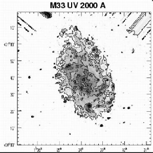
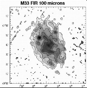
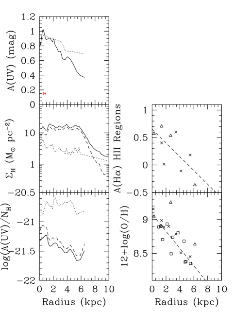
Figure 1: Profiles in M33. Top row-left column : UV attenuation radial profile obtained from the FIR to UV ratio (solid). The dotted curve indicates the integrated extinction within the radius $R$. The error bar indicates the resolution (IRAS resolution at 100 $\mu$m). Middle row-left column: hydrogen density profiles (neutral: dashed, molecular: dotted, and total:solid). Bottom row-left column: $A(UV)$ to hydrogen atom column density (neutral: dashed, molecular: dotted, and total:solid). Middle row-middle column: H$\alpha$ extinction in HII regions (different symbols correspond to different data references (Table 3), and fit (dashed line). Bottom row-middle column: oxygen abundance in HII regions and fit (dashed line). On the right, the UV (top) and IRAS 100 $\mu$m (bottom) surface brightness images are shown. The contours are separated by 1 mag arcsec^-2 in both images where $\mu$=-2.5 log($F$)+15 ($F$ in Jy arcsec^-2) for the 100 $\mu$m image and $\mu_{UV}$=-2.5 log($F$)-21.175 ($F$ in erg cm^-2 s^-1 A^-1 arcsec^-2) for the 2000 Å image.

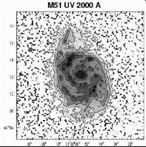
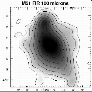
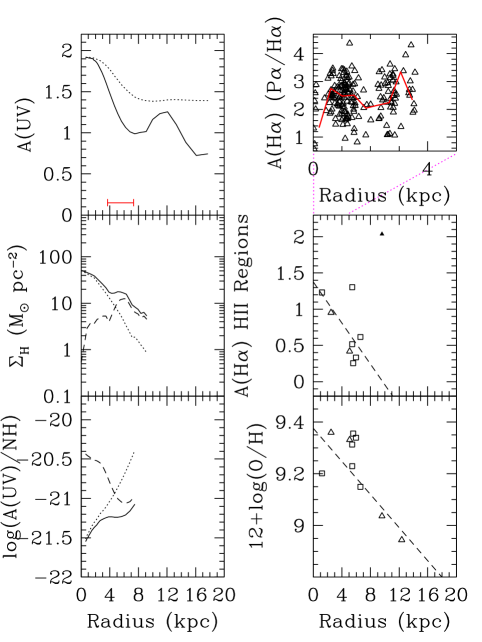
Figure 2: Profiles in M51. Same caption as for Fig. 1 except: top row-middle column: H$\alpha$ extinction derived from Paschen-$\alpha$ to H$\alpha$ ratio, individual HII regions from Scoville et al. (2001) (triangles). The line is obtained by averaging the P$\alpha$ and H$\alpha$ fluxes in 10 arcsecs radial bins, taking into account only the pixels with signal to noise larger than 5 and 3 in respectively the P$\alpha$ and H$\alpha$ images of Scoville et al. (2001).

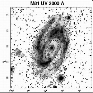
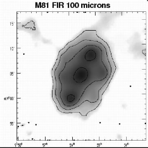
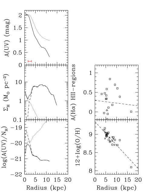
Figure 3: Profiles in M81. Same caption as for Fig. 1.

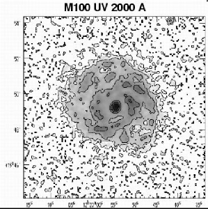
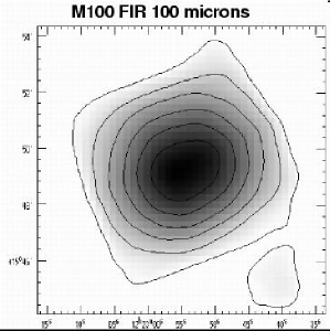
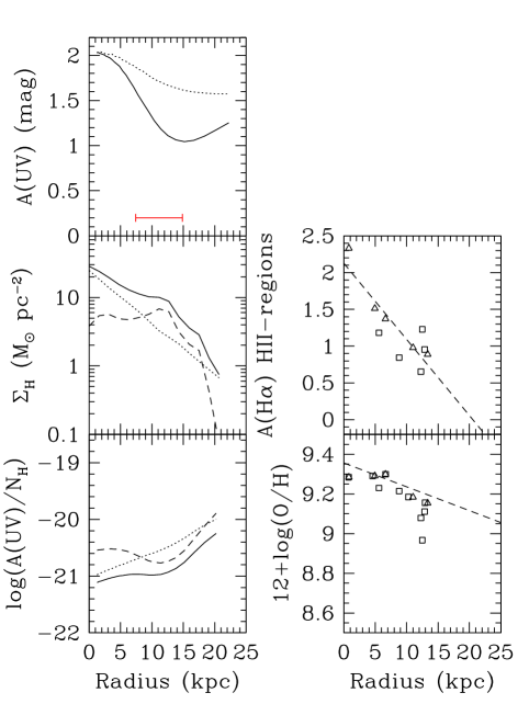
Figure 4: Profiles in M100. Same caption as for Fig. 1.

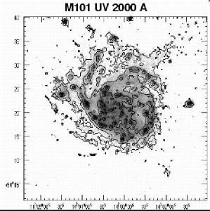
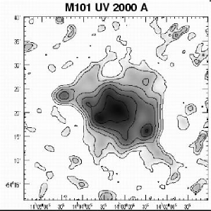
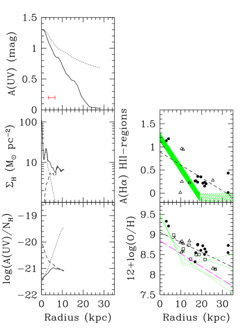
Figure 5: Profiles in M101. Same caption as for Fig. 1 except: Middle row-middle column: The shaded area indicates roughly the extinction gradient derived by Scowen et al. (1992) from their narrow-band imaging study. Bottom row-middle column: The dotted lines indicate the gradients of Scowen et al. (1992) for the various values of the surface brightness threshold they use with their narrow-band imaging. The long-dashed line is the gradient of Kennicutt et al. (2003) measured with high signal-to-noise data (and thus avoiding the use of strong-line calibrations as in the other studies).

2.2 Abundances in HII regions

Table 3: References for complementary data, Position Angle ($PA$) and inclination ($incl$) in degrees used for determining the profiles

	HI	CO	HII regions	$PA$	$Incl$
M33	1	7	10,11,12(21)	22	55
M51	2	8	10,13(10)	17	20
M81	3	9	14,15,16(28)	-28	59
M100	4	8	10,17(14)	153	27
M101	5	5	10,18,19,20(38)	42	21
M106	6	8	14,21(20)	-30	63

References for the HI. [1]: Deul & van der Hulst (1987). [2]: Rand et al. (1992). [3]: Rots (1975). [4]: Warmels (1986). [5]: Wong & Blitz (2002). [6]: Wevers et al. (1986). References for the CO. [7]: Corbelli (2003) [8]: Young et al. (1995) [9]: Sage (1993) [5]: Wong & Blitz (2002). Spectral information for HII regions (for abundances and extinctions). The number between parentheses indicates the number of HII regions. [10]: McCall et al. (1985). [11]: Kwitter & Aller (1981). [12]: Vilchez et al. (1988). [13]: Diaz et al. (1991) [14]: Oey & Kennicutt (1993). [15]: Garnett & Shields (1987). [16]: Stauffer & Bothun (1984). [17]: Shields et al. (1991). [18]: Smith (1975). [19]: Rayo et al. (1982). [20]: van Zee et al. (1998). [21]: Zaritsky et al. (1994)

The abundances are computed for the individual HII regions of each galaxy. The references for the HII regions data are given in Table 3. As most ot them were already collected by Zaritsky et al. (1994) (and used to compute gradients), the abundances of oxygen (12+log(O/H) are computed from the R23 indicator ([OII]3726,3729+[OIII]4959,5007)/H$\beta$, using their calibration.

For each galaxy, these abundances exhibit a clear gradient, shown as the dashed line in the bottom row-middle column panel of Figs. 1 to 6. This fit will be used hereafter to determine the abundance at a given radius in each galaxy. We implicitly make the assumption that the oxygen abundance measured in HII regions is the same as in all the interstellar medium at the same distance from the centre of the galaxy.

In the case of M101, we also show the oxygen abundance gradients deduced by Scowen et al. (1992) from their analysis of 625 HII regions (dotted lines). The different curves correspond to different surface brightness thresholds that they apply to select the HII regions. The advantage of the gradients of Scowen et al. (1992) is the large number of HII regions involved, although computed with limited spectral information. Contrary to other studies, they propose a two slope gradient, but the abundances are nevertheless close to those derived from the spectroscopy of the limited number of HII regions of Table 3.

With high signal-to-noise spectra of 20 HII regions, Kennicutt et al. (2003) recently derived the electron temperature for those HII regions and determined robust abundances which are systematically lower (by 0.2-0.5 dex) than the abundances obtained with strong lines and empirical calibrators. Figure 5 shows that the Kennicutt et al. (2003) gradient is also slightly steeper that from the strong-lines.

Since we do not have other data for the rest of our galaxies, we use the abundance gradient as derived from the R23 calibration (including M101, for the sake of homogeneity). If R23 systematically produces abundances that are too large, our results should be corrected accordingly, perhaps by reducing our abundances by a few tenths of dex.

The uncertainty in the abundances is usually on the order of $\sim$ 0.15 dex. This is much smaller than the differences in the metallicity measured at various radii, so that the value of the gradient is relatively well defined.

2.3 Gas profiles

The molecular profiles are computed from the $I(CO)$ profiles; references are given in Table 3. When only a few points are available, an exponential profile is fitted and used afterwards. We use a conversion factor $X$ from $I(CO)$ to H₂ dependent on the metallicity, as suggested by Boselli et al. (2002):

$$logX=-1.01(12+log(O/H))+29.28.$$ (1)

This correlation was found for integrated values over whole galaxies and is here assumed to hold for radial profiles as well. Note that Nakai & Kuno (1995) found similar results in M51 in their analysis of the radial variation of the dust-to-gas ratio. The value of $12+log(O/H)$ used in Eq. 1 is the one given by the radial fit of the abundance gradient (see Sect. 3).

References for the atomic gas profiles are given in Table 3. Although these profiles are given at various resolutions, the results of our analysis should not be affected since all our profiles are smoothed to the IRAS 100 $\mu$m resolution in order to compare them with the derived UV attenuation. For each galaxy, the gas profiles are shown in the middle row-left column panels of Figs. 1 to 6.

2.4 FIR and UV profiles

Figure 7: Profiles of UV and FIR surface brightness at the IRAS 100 $\mu$m resolution ($\sim$ 100 arcsec). For the infrared, $\mu$ is defined as -2.5 log ($F$) + 15, $F$ in Jy arcsec^-2. In the UV $\mu_{UV}$=-2.5 log($F$)-21.175, $F$ in erg cm^-2 s^-1 A^-1 arcsec^-2.

From the IRAS and FOCA images, we compute the surface brightness profiles at 2000 Å, 60 and 100 $\mu$m as follows. After removing the stars present in the UV image and subtracting the sky, the resolution in all images is changed to that of the 100 $\mu$m maps (100 ”) by convolution with a Gaussian filter. The pixel size of the UV image is changed to match IRAS (15 arcsecs per pixel).

The fluxes are azimuthally averaged using the task ELLIPSE within IRAF, keeping the centre, ellipticity and position angle fixed for each galaxy. We adopt the same position angle and inclination as used in the determination of the HI profiles, and given in Table 3.

The UV profiles are corrected for Galactic extinction as taken from Schlegel et al. (1998).

The resulting surface brightness profiles are shown in Fig. 7 (for the FIR, we adopt $\mu$= -2.5 log ($F$) + 15, $F$ in Jy arcsec^-2). We truncate the profiles at a radius where the azimuthally averaged flux surface densities become lower than one sigma of the sky.

Our profile of M33 is in agreement with the one published by Buat et al. (1994) at the FOCA spatial resolution, but shows less structure because our data have been smoothed.

The profile of M106 shows a flattening in the outer part of the UV and 60 $\mu$m flux. The feature must be real since we are well above the sky in the UV and it is located in the area of a ring, clearly visible in the image. At 60 $\mu$m, the flux at the same radius is barely more than one $\sigma_{sky}$, and is dominated by a few large peaks, not present in the 100 $\mu$m image. The few outer points of this profile are quite uncertain.

3 Radial extinction profiles

The extinction profile $A(UV)$ is determined from the FIR/UV ratio by combining the UV and FIR radial profiles (determined as described in Sect. 2.4), using the calibration of Buat et al. (1999), in Sect. 3.1. By combining these results with a simple geometrical model, we give in Sect. 3.2 a simple recipe to extend A(UV) to optical and NIR wavelengths.

3.1 Determination of the UV extinction profile

To compute the UV extinction $A(UV)$, we adopt an updated version of the fit of Buat et al. (1999) given in Iglesias et al. (2003):

$$A(UV)=0.622 + 1.140\ log\left(\frac{F_{FIR}}{F_{UV}}\right)$$ (2)

$$+ 0.425\left(log\left(\frac{F_{FIR}}{F_{UV}}\right)\right)^{2},$$

where $F_{FIR}$ (W m^-2 arcsec^-2) is obtained from a combination of the 60 and 100 $\mu$m fluxes, i.e.:

$$F_{FIR}=1.26(2.58\,10^{12}f_{60}+10^{12}f_{100})10^{-26}$$ (3)

where $f_{60}$ and $f_{100}$ are the IRAS surface brightnesses in Jy arcsec^-2; and $F_{UV}$ is the UV flux:

$$F_{UV}=2000\,10^{-3}f_{2000}[{\rm Wm^{-2}arcsec^{-2}}]$$ (4)

where $f_{2000}$ is the UV surface brightness (erg cm^-2 s^-1 Å^-1 arcsec^-2).

The IRAS FIR does not include the total dust emission. However, the calibration of Iglesias et al. (2003), using the ISO (Infrared Space Observatory) results of Dale et al. (2001), takes into account the average difference between the FIR emission and the total dust emission in disk galaxies. This extrapolation is nevertheless based on data short-ward of 100 $\mu$m and model SED curves and does not take into account the radial variation of the dust temperature. Alton et al. (1998), using ISO, found that the cold dust is indeed more extended than the warm dust in their sample of disc galaxies. We assume that the energetic balance is not much affected by this radial change, and implicitly use an average calibration (note that our 60/100 ratio does not exhibit a large gradient).

The FIR to UV ratio is believed to be a robust method of determining $A(UV)$ (e.g. Witt & Gordon 2000). Other calibrations of the determination of the UV extinction from this ratio have been proposed by Panuzzo et al. (2003) for face-on and edge-on orientations. As our galaxies are quite far from being edge-on (inclinations from 20 to 63 ^∘), we compared our results with the $A(UV)$ obtained for the face-on calibration of Panuzzo et al. (2003). The difference in A(UV) using the two methods is less than 10 % except for extinctions lower than a few tens of magnitude, as in the few outer points of M101 (for a radius larger than $\sim$ 20 kpc, see Fig. 5), confirming that the determination of A(UV) is mostly independent on the adopted calibration.

An implicit assumption in using the FIR/UV ratio is that we take into account all the UV photons which may have heated the dust where it radiates the energy (after having eventually propagated inside the galaxy). While this is not the case for regions as small as HII regions, it is certainly true for the integrated flux of galaxies. In the resolved galaxies, this method can still be applied provided that we average the flux over large enough areas, as for the case of our sample where the azimuthally averaged profiles are determined within 100 arcsec wide annuli (between $\sim$ 0.5 and $\sim$ 8 kpc in our galaxies), the IRAS 100 $\mu$m resolution.

In the top-left panels of Figs. 1 to 6, the resulting profile of the UV extinction $A(UV)$ is shown as a solid line (the dotted line indicates the extinction integrated within the radius $R$, obtained by applying Eq. 2 to the integrated fluxes within the ellipses of semi-major axis $R$).

For all the galaxies, we observe a clear UV extinction gradient over a radial range several times the resolution. Only for M51 is a secondary peak observed, whose radius corresponds to its companion galaxy. Indeed the companion suffers very strong extinction since it is not visible in the UV image while being prominent in FIR. The UV and FIR surface brightness measured in the images at the position of the companion give a local extinction of $\sim$ 3 magnitudes.

Figure 8: Relation between the absorption A_i and the optical thickness $\tau_{i}$ for sandwich models of various dust to star scale-height ratios $\xi$.

3.2 A simple model to derive the optical thickness and the extinction profile at various wavelengths

$A(UV)$ can be scaled to $A(\lambda)$ at any wavelength $\lambda$ once an extinction law (Galactic, Magellanic) and a geometry are assumed. To simplify the formalism and to be consistent with previous studies (e.g. Boselli et al. 2003), we assume a Galactic extinction law and a sandwich model with a wavelength dependent dust-to-star scale-height ratio $\xi$. The extinction $A$ (in magnitude) then depends on the optical thickness ($\tau$) via Eq. 5:

$$A_{i}=-2.5log\left(\left(\frac{1-\xi}{2}\right)(1+e^{-\tau_{i}})+\left(\frac{\xi}{\tau_{i}}\right)(1-e^{-\tau_{i}})\right).$$ (5)

$\tau_{i}$, $A_{i}$, and $\xi$ are wavelength-dependent. $\tau_{i}$ and $A_{i}$ correspond to a given inclination, i.e. $\tau_{i}=\tau_{0}sec(i)$. The relation between $A_{i}$ and $\tau_{i}$ is shown in Fig. 8 for several values of $\xi$.

We numerically invert Eq. 5 to derive the profile of $\tau_{UV}$ from the one of $A(UV)$. Then, we compute the optical thickness at a given wavelength as : $\tau_{\lambda}=\tau_{UV}\ k(\lambda)/k(UV)$, where $k$ is a typical Galactic extinction curve ($R_{V}=A_{V}/E(B-V)$=3.1). The choice of this extinction curve is justified by the fact that the metallicity in our galaxies (see Table 2 and Fig. 13, for instance) is larger than in the Magellanic Clouds. We are implicitly assuming that the albedo does not depend strongly on the wavelength and that the scattering is isotropic (we also tried to include the effects of the albedo and phase function as in Calzetti et al. (1994) with very similar results).

We can then compute the extinction at any wavelength with the help of Eq. 5. We show the result of this operation for the V and H band wavelengths in Fig. 9. We adopt a dependence of the dust-to-star scale-height ratio on wavelength as suggested by Boselli et al. (2003):

$$\xi(\lambda)=1.0867-5.501\ 10^{-5}\lambda(\AA),$$ (6)

This assumption is used to mimic the fact that the young stars (predominantly emitting at short wavelengths) lie in a thinner disk (similar to the dust, $\xi$=1 at 2000 Å) than older stars (emitting at long wavelengths) which migrate to larger heights with age. This is in agreement with some observations (Boselli & Gavazzi 1994), but not always confirmed for edge-on nearby galaxies (e.g. Xilouris et al. 1999).

Note that a sandwich model with a constant dust-to-star scale-height ratio $\xi(\lambda)$=0.5 is not consistent with the observations. It can be seen in Fig. 8 that for this value of $\xi$, the absorption in magnitudes can reach only moderate values. Even for infinite optical thickness, we would obtain only $A(UV)$=1.5 which is lower than the absorption measured in the centres of M51, M81 and M100.

The results of this model applied to our galaxies are shown in Fig. 9 for the wavelengths of the V and H bands.

The variation of extinction with radius that we can detect is between $\sim$ 0.5 and $\sim$ 1 mag over the whole radial range in the UV. The results of the model indicate that the typical V band extinction gradient is between 0.2 and 0.5 mag, and it is very small in the H band. Of course this is model-dependent and could easily vary by a few tenths of magnitude in the V band if we change $\xi$.

Fig. 9 also shows the extinction profiles in V and H when a simple screen of Milky Way-like dust is adopted (marked “S” in the figure) or with the Calzetti (1999) law (“C”). The differences between these models are negligible at long wavelengths but can reach 0.3 magnitude in V (and eventually change with the radius).

This shows that the geometry (and the choice of one geometrical and dust model rather than another) can have an important impact on the determination of the colour gradient of the underlying stellar population, even if the observed colour gradient is unlikely to be mainly due to the dust (de Jong 1996). The extinction dependence on the geometry is a well known effect, studied in detail in Disney et al. (1989).

3.3 Comparison with other studies of M51

Hill et al. (1997) show a UV colour profile of M51 ($\mu_{151}$-$\mu_{U}$) varying by 1 mag or so between $\sim$ 2 and 12 kpc (the gradient is even stronger if smaller radii are included, but we cannot probe such small scales with our resolution). Hill et al. propose that the colour gradient is due to an extinction gradient. We indeed find (in a more direct way) an extinction gradient in the UV in M51 (Fig. 2).

Vansevičius (2001) estimates the extinction at 11 kpc from the centre of M51 using its companion as a tracer. He finds A_V = 0.7 $\pm$ 0.3 mag. The extinction we derive from our model at this radius is a bit lower ($\sim$ 0.5 mag) but within the error bars (see Fig. 9). As another illustration of the dependence of our results on the adopted geometry, changing $\xi$ to a constant value of 0.7 (independent of the wavelength) would increase the value of A_V by only 0.1 magnitude (larger differences would occur where the optical thickness is larger, i.e. in the inner few kpc of the galaxy).

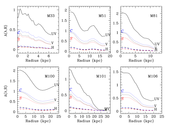
Figure 9: Extinction profiles in the UV, V and H. $A(UV)$ is obtained from the FIR/UV ratio. The black line shows the extinction profiles in V and H as derived for a sandwich model with dust to star scale-height ratio $\xi$ depending on the wavelength. For each of these two bands, the others curve show the predicted extinction for a dust screen with Milky-Way-type dust (S) and the Calzetti (1999) law (C).

4 Extinction in the UV continuum and in HII lines: A(H$\alpha$) vs A(UV)

To check the consistency of our extinction determination with average values available in the literature, we estimate the total integrated extinction for both the UV and H$\alpha$ and compare them to the results of Buat et al. (2002) for late-type normal spirals.

The integrated UV extinction within the radius where it is computed can be seen as the dotted curve in the top-left panels of Figs. 1 to 6. It usually presents a plateau or a small decrease at large radii; we then consider as “integrated” extinction over the whole galaxy its value at the largest radius. We choose as a typical H$\alpha$ extinction the average of A(H$\alpha$) found in the HII regions considered in this study.

The average H$\alpha$ extinction (and its standard deviation) and the UV integrated extinction are compared in Fig. 10. This figure also shows the local values (at different radii) within each galaxy connected by a curve. The integrated value is representative of an “average” of the local values obtained at different radii. The filled circles are the star-forming galaxies of Buat et al. (2002), using the updated H$\alpha$ extinction of Gavazzi et al. (2004) (which introduces small differences with respect to Buat et al.).

Our “average” values (squares) and most of the profiles (curves) largely overlap the points of Buat et al. (2002), however, we span a limited range of extinction than they do since we are limited to absorptions less than 2 mag, while Buat et al. include objects with up to $\sim$ 4 magnitudes. Actually, this is the case of M100 for which Buat et al. find $A(H\alpha)>$ 3.7 mag. However, they notice that this high value may be due to the very high surface brightness nucleus while the disk might be less extincted. Our H$\alpha$ extinction derived from HII regions in the disk is indeed lower.

An important difference between our approach and that of Buat et al. (2002) is that we defined an average $A(H\alpha)$ in HII regions, while their integrated value is dominated by high surface brightness regions and the nucleus. This might explain the differences between the two studies and especially why our “local” study does not reach the high values found by Buat et al. (2002) in “integrated” galaxies.

We can also see in Fig. 10 that lower values of the integrated UV extinction are found for M33 and M101 (which are of type Scd) than for the other galaxies (type Sbc and Sab). The average values for these two groups are in agreement with (albeit slightly lower than) the average values given by Boselli et al. (2003) for Sc-Scd (0.85 mag), and for Sa-Sbc galaxies (1.28 mag), obtained for a much larger number of integrated galaxies.

The profile of M81 in $A(H\alpha)$ is rather flat, as seen in Fig. 10. It can be seen in Fig. 3 (middle row-middle column panel) that this is due to a large scatter of the extinction in a limited number of HII regions. In general, the average values of $A(H\alpha)$ (squares in Fig. 10) are more robust than the local values as the latter are more sensitive to the small number of HII regions.

Finally, we also show in Fig. 10 the Calzetti (1997) attenuation law for starbursts ($A(UV)=1.6A(H\alpha)$, see Buat et al. 2002, for the derivation) The relation is steeper for the integrated star-forming galaxies, as shown in Buat et al. (2002), although consistent, within the large uncertainties, with local values.

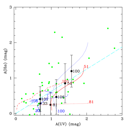
Figure 10: UV vs H$\alpha$ extinction. The squares are the average values for each galaxy. The curves are local values at different radii within each galaxy. Filled circles are the star-forming galaxies of Buat et al. (2002) (adopting the $A(H\alpha)$ of Gavazzi et al. 2004), computing $A(UV)$ from the UV/FIR ratio, like for our galaxies, but using integrated fluxes. The long dashed line indicates the relation $A(UV)=1.6A(H\alpha)$, expected in the case of the attenuation law proposed by Calzetti (1997) for starbursts.

5 Extinction, metals, and gas

5.1 Dependence of the extinction on the metallicity

Quillen & Yukita (2001), using extinction derived from the Paschen-$\alpha$ (P$\alpha$) to H$\alpha$ ratio in the centres of a few galaxies and along the profiles of M51 and M101 (with original data from the thesis of Scowen 1992), found that the extinction correlates with the metallicity and with the gas surface density (their Fig. 4). Heckman et al. (1998) have shown a dependence of the UV spectral slope $\beta$ on O/H in their starbursts galaxies ($\beta$ is defined as $F(\lambda)\propto\lambda^{\beta}$ for $1250<\lambda<2600$ Å by Calzetti et al. (1994) and is equal to $\sim$ -2.1 for a dust-free starburst). Several studies, theoretical and observational, have tried to relate the amount of extinction to metallicity and gas amount (e.g.; Issa et al. 1990; Lisenfeld & Ferrara 1998; Dwek 1998; Hirashita et al. 2001).

From eq. 5 (adopting the varying dust-to-star scale-height $\xi$, as given in Eq. 6) we derive for each profile of $A(UV)$ the corresponding profile of $\tau_{UV,i}$, which is corrected for inclination, to obtain $\tau_{UV,0}$.

In Fig. 11 (bottom), we superpose the relation between the optical thickness $\tau_{UV,0}$ and the abundance for all the galaxies. In the top panel, we directly plot the extinction $A(UV)$ in magnitudes (uncorrected for inclination) as a function of the oxygen abundance. The advantage of using $A(UV)$ as derived from the FIR to UV flux ratio with respect to other dust extinction indicators is that it does not depend on the extinction model. A quite good correlation between the extinction and the metallicity is observed,

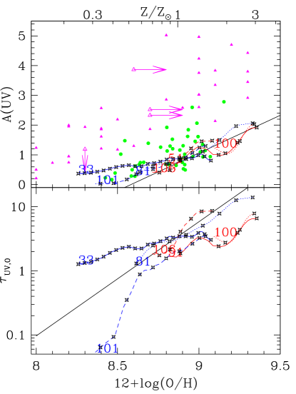
Figure 11: UV Extinction (top) and optical thickness (bottom) as a function of 12+log(O/H). Each galaxy is represented by a curve. The symbols correspond to radii separated from each other in units of the spatial resolution. The median of a fit performed on each galaxy is shown as black line. In the top panel, we also show the extinction derived for the integrated starbursts of Heckman et al. (1998) as triangles and the star forming galaxies of Buat et al. (2002) as circles.

suggesting that the extinction does depend on the metallicity. This dependence is confirmed by the UV extinctions of the integrated star forming galaxies of Buat et al. (2002), shown as circles, adopting the metallicities of Gavazzi et al. (2004, and in preparation), although with a larger scatter. This correlation between local extinctions and metallicities amongst our different galaxies is a striking result as the oxygen abundance and $A(UV)$ are obtained independently of each other.

Actually, a dependence of the UV extinction on the metallicity was already suggested by Heckman et al. (1998) for their starburst galaxies. We show their data as triangles in the same figure. Following Buat et al. (2002), the $A(UV)$ extinction at 2000 Å in starbursts is computed as

$$A(UV)=0.9\times 2.5\,\,log\left(\frac{1}{0.9}\,\frac{F_{FIR}}{F_{UV,1600\AA}}+1\right).$$ (7)

The extinction in starbursts is much larger for the same metallicities and shows a larger scatter than what we find within the disks of our spirals, as already remarked by Buat et al. (2002).

The black lines are the median of the fit performed for each of our galaxies. The numbers given in parentheses in eq. 8 indicate the standard deviation in the parameters found for each galaxy. These numbers reflect the large differences between galaxies, nevertheless the global trend is well established.

$$log(\tau_{UV,0}) = -15.25(\pm 6.27)+1.78(\pm 0.70)\times Z$$

$$or:$$ (8)

$$A(UV) = -21.80(\pm 11.70)+2.54(\pm 1.28)\times Z$$

where $Z=12+log(O/H)$. The standard deviations of $\tau$ and $A(UV)$ around the median-fit are $\sigma$=0.37 and 0.43 respectively.

The large scatter produces an important uncertainty in the zero-point of this relation, even though the dependence on the metallicity is well defined. These relations could be used to predict $\tau$ (or $A(UV)$) as a function of the radius for each galaxy with an available abundance gradient. In the case where no abundance gradient is available, we can use the fact that the abundance gradient is constant in units of the disc scale-length (Prantzos & Boissier 2000; Henry & Worthey 1999, and references within). The oxygen gradient is typically -0.2 dex / $R_{B}$ ($R_{B}$ is the disk scale-length in the blue band). The zero point of the relation can be determined from the magnitude-metallicity relationship. Garnett (2002) has shown that the oxygen abundance at the effective radius in spiral galaxies satisfies:

$$[log(O/H)]_{Reff}=-0.16M_{B}-6.4$$ (9)

where $M_{B}$ is the blue absolute magnitude. For an exponential disk, $R_{eff}=1.865R_{B}$. Combining this result with Eq. 8, we obtain a second expression of the optical thickness with no explicit dependence on the abundance gradient:

$$log(\tau_{UV,0}) = -0.28(\pm 0.11)M_{B}-0.36(\pm 0.14)\frac{R}{R_{B}}$$

$$- 4.62(\pm 10.45)$$

$$or:$$ (10)

$$A(UV) = 0.40(\pm 0.20)M_{B}-0.51(\pm 0.25)\frac{R}{R_{B}}$$

$$- 6.60(\pm 19.38)$$

These relations can be used for any galaxy with an absolute magnitude $M_{B}$ and scale-length $R_{B}$. The uncertainties given in Eq. 10 are obtained only by propagating the uncertainties of Eq. 8.

To check the validity of Eq. 8 for computing an extinction profile from the abundance gradient, in the top-panel of figure 12, we show as a function of radius the difference between the extinction deduced from the FIR/UV ratio ($A(UV)_{FIR/UV}$) and the one deduced from the oxygen abundance at this radius ($A(UV)_{O/H}$). The bottom panel shows the ratio of the two optical thicknesses.

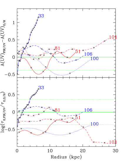
Figure 12: Top: Radial profiles of the difference between $A(UV)$ deduced from the FIR/UV ratio and $A(UV)$ obtained by applying Eq. 8 to the oxygen abundance. Bottom: radial profile of the ratio of the optical thickness deduced from the FIR/UV ratio to the one obtained by applying Eq. 8 to the oxygen abundance. The horizontal lines show the average value and $\pm$ one $\sigma$.

The optical thickness “predicted” by applying Eq. 8 to the oxygen abundance, $\tau_{0,O/H}$, is within a factor two of the “observed” one $(\tau_{0,FIR/UV})$ for most of the points. Large departures are found only for the case of M33, which is the galaxy with the smallest metallicity in our sample.

Similarly, the $A(UV)_{O/H}$ deduced from the metallicity is frequently found at $\sim$ 0.3 mag from $A(UV)_{FIR/UV}$ and the largest deviation is for M33 (up to more than one magnitude in its outer parts). This may indicate that our relations are valid only in the high-metallicity domain.

The points situated at radii larger than $\sim$ 20 kpc also show large differences between the predictions and the observations. However, these data only concern the outer part of one galaxy (M101) where $A(UV)$ is very small anyway (and where the calibration of our method is not as secure: see Sect. 3.1). In any case, deviations from the average relation in the external parts are expected since the uncertainties on the profiles (especially in the FIR) are larger.

5.2 Dust-to-Gas ratio

The extinction-to-gas ratios (bottom-left panel of Figs. 1 to 6) are computed from the gas profiles (middle row-left column), after smoothing the resolution to the IRAS 100 $\mu$m maps. This ratio shows various values and trends for each galaxy.

Based on extinction measured in HII regions at various radii, Issa et al. (1990) suggested that the dust-to-gas ratio depends on the metallicity. This is quite natural since the dust is formed from metals and the mass of metals is equal to the product of the metallicity and the gas mass. This trend is naturally obtained in the framework of models computing consistently the evolution of metals and dust, despite the large uncertainties in the yields of both (e.g. Inoue 2003; Dwek 1998).

Guiderdoni & Rocca-Volmerange (1987) used the the solar neighborhood and the Magellanic Clouds to propose the relation $\tau_{\lambda}/N_{H}\propto(Z/Z_{\odot})^{s}$ with s $\sim$ 1.35 (1.6) for wavelengths shorter (longer) than 2000 Å, ($N_{H}$ represents the total hydrogen column density).

As can be seen in Fig. 13 (top), we obtain a similar trend, although with a large dispersion, especially for the metal-rich part.

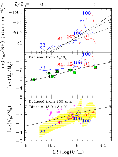
Figure 13: Top: Optical thickness to hydrogen column density ratio. The short-dashed line is a fit to our data of slope 0.88. The long-dashed lines show the metallicity dependence of the dust to gas ratio of Guiderdoni & Rocca-Volmerange (1987). middle: dust to gas mass ratio (computed from the $A_{V}/N_{H}$ ratio as explained in Sect. 5.2) as a function of metallicity. The circles mark the integrated galaxies of Issa et al. (1990). The solid curve is the best-fit model of Hirashita et al. (2001). bottom: dust to gas mass ratio (computed from the 100 $\mu$m flux density). The crosses indicate the integrated galaxies of Tuffs et al. (2002) and Contursi et al. (2001). The solid curve is the best-fit model of Hirashita et al. (2001).

A formal fit (short dashed line in Fig. 13) to our data gives a slope of 0.88. This is lower than the values proposed by Guiderdoni & Rocca-Volmerange (1987), which are illustrated by the two long-dashed lines in Fig. 13. Note however that we apply different methods (FIR/UV ratio, metallicity dependent CO to H₂ conversion factor…) and probe different ranges of metallicities as our spirals are more metal-rich than the Magellanic Clouds.

Following Hirashita et al. (2001), we can convert our optical-thickness-to-hydrogen ratio into a dust-to-gas mass ratio. This is done by using the profiles of $A_{V}$ (Fig. 9, computed with the model of Sect. 3.2) and assuming that $M_{D}$/$M_{G}$ (the dust-to-gas mass ratio) is equal to 6 $\times$ 10^-3 when $N_{H}/E(B-V)$=5.9 10²¹ (Hirashita et al. 2001, and references within). The results are shown in the middle panel of Fig. 13. In this figure, we compare our results with the dust-to-gas mass ratio found by Issa et al. (1990) for 6 galaxies. They were deduced from the $A_{V}/N_{H}$ of HII regions (or galaxy counts and interstellar absorption in the Milky Way), estimated at a radius of 0.7 $R_{dV}$ ($R_{dV}$ is from de Vaucouleurs et al. 1976).

Three of the galaxies of Issa et al. (1990) are in common with our study (M33,M51,M101), presenting some differences with our results that must come from the fact that we derive $A_{V}$ from the FIR/UV ratio and use the gas profile, while they use measurements done in HII regions. In M101, our metallicity is higher, but our gradient is based on several, more recent studies.

A more direct way to estimate the dust-to-gas mass ratio is to deduce the dust mass from the FIR flux. We compute the dust mass following Devereux & Young (1990) with the same numerical coefficient as in Boselli et al. (2002):

$$M_{D}=1.27F_{100}D^{2}(exp(144/T_{D})-1)M_{\odot}.$$ (11)

The mass is very sensitive to the dust temperature $T_{D}$ which is still poorly constrained by the 100 $\mu$m IRAS data. In the bottom-panel of Fig. 13 we show as crosses the dust-to-gas mass ratio obtained from the ISO measurements of integrated flux densities of galaxies by Tuffs et al. (2002) and Contursi et al. (2001), where the metallicity is from Gavazzi et al. (2004). We adopt the average temperature ($T_{D}$=18.9 K) of the sample of Tuffs et al. (2002) (for which the dust temperatures are given in Popescu et al., 2002) to compute the dust-to-gas mass ratio of our galaxies at different radii. This temperature is consistent with the 200 $\mu$m observations of Alton et al. (1998). The result is shown in the same figure as a function of the metallicity. The shaded area indicates a dispersion of $\pm$ 3.7 K.

The dust-to-gas ratio is lower than the one deduced from the $A_{V}/N_{H}$ and shows a clearer trend with metallicity, still with a large dispersion.

If a dust temperature gradient is present (with higher $T_{D}$ in the center of galaxies than in their outskirts), as expected from the observed gradient in metallicities and star formation rate (and suggested by the ISO observations of e.g. Alton et al., 1998), it would flatten the relation between the dust-to-gas mass ratio and the metallicity, making it more similar to the one derived from the $A_{V}/N_{H}$ ratio (see bottom panel).

The best-fit model of Hirashita et al. (2001) is indicated in the figure by the solid curve. It reproduces the global trend of increasing dust-to-gas ratio from dwarfs (Lisenfeld & Ferrara 1998) to spirals (Issa et al. 1990).

When a dust-to-gas ratio is determined as in Issa et al. (1990), the trend for our galaxies is weaker than in this model, and a great deal of diversity is observed amongst the galaxies. The values obtained from the 100 $\mu$m surface brightness are in slightly better agreement with the model. The uncertainties due to the temperature (shaded area) and its gradient (see discussion above) are however large.

6 Conclusion

We have combined 2000 Å UV images obtained with FOCA, and FIR IRAS images at 60 and 100 $\mu$m to compute the FIR and UV profiles of six nearby late-type galaxies. We used the FIR/UV ratio to trace the radial variation of the UV extinction in each galaxy. We detect a monotonic gradient of decreasing extinction with the radius in all of them, except in M51 where the companion produces a second peak in the averaged profile.

These extinction profiles were compared to the extinctions derived from hydrogen lines (mainly the Balmer decrement) in HII regions and we studied the relation between the extinction, the gas surface density, and the metallicity.

The most significant result of this analysis is a clear correlation between the UV extinction (in magnitudes or in optical thickness) and the metallicity deduced independently from the FIR/UV profile and the abundance gradient respectively. This correlation is also found in the integrated star forming galaxies of Buat et al. (2002) (a similar relationship was found in starbursts (Heckman et al. 1998), but with larger scatter and higher extinction for a given metallicity).

A fit to our azimuthally averaged data provides a simple relationship between the extinction in the UV and the metallicity in galaxies for which an abundance gradient is available (Eq. 8). Coupling this result with the mass-metallicity relationship, we derived an empirical formula linking the extinction profile to the blue absolute magnitude and disc scale-length of galaxies (Eq. 10). Once the UV extinction profile is determined by one of the previous methods, the extinction profile at any wavelength can easily be derived through a simple model as the one described in Sect. 3.2.

Our results were obtained with a very limited sample of galaxies. In the future, we will however be able to extend this work with the new images of GALEX in the UV and SIRTF in the far-infrared for a larger number of galaxies. GALEX data are being used to study the extinction radial profile in individual spirals: in M83 (Boissier et al., 2004) and in a comparative study with ISO FIR maps for M101 (Popescu et al., 2004).

References

- Alton et al. (1998) Alton, P. B., et al. 1998, A&A, 335, 807
- Bell (2002) Bell, E. F. 2002, ApJ, 577, 150
- Bohlin et al. (1978) Bohlin, R. C., Savage, B. D., & Drake, J. F. 1978, ApJ, 224, 132
- Boissier et al. (2004) Boissier et al., 2004, ApJL GALEX issue, in preparation
- Boselli & Gavazzi (1994) Boselli, A. & Gavazzi, G. 1994, A&A, 283, 12
- Boselli et al. (2002) Boselli, A., Lequeux, J., & Gavazzi, G. 2002, A&A, 384, 33
- Boselli et al. (2003) Boselli, A., Gavazzi, G., & Sanvito, G. 2003, A&A, 402, 3
- Buat & Xu (1996) Buat, V., & Xu, C. 1996, A&A, 306, 61
- Buat et al. (1999) Buat, V., Donas, J., Milliard, B., & Xu, C. 1999, A&A, 352, 371
- Buat et al. (2002) Buat, V., Boselli, A., Gavazzi, G., & Bonfanti, C. 2002, A&A, 383, 801
- Calzetti et al. (1994) Calzetti, D., Kinney, A. L., & Storchi-Bergmann, T. 1994, ApJ, 429, 582
- Calzetti (1997) Calzetti, D. 1997, The Ultraviolet Universe at Low and High Redshift: Probing the Progress of Galaxy Evolution, 403
- Calzetti (1999) Calzetti, D. 1999, Ap&SS, 266, 243
- Calzetti et al. (2000) Calzetti, D., Armus, L., Bohlin, R. C., Kinney, A. L., Koornneef, J., & Storchi-Bergmann, T. 2000, ApJ, 533, 682
- Caplan & Deharveng (1986) Caplan, J. & Deharveng, L. 1986, A&A, 155, 297
- Charlot & Fall (2000) Charlot, S. & Fall, S. M. 2000, ApJ, 539, 718
- Contursi et al. (2001) Contursi, A., Boselli, A., Gavazzi, G., Bertagna, E., Tuffs, R., & Lequeux, J. 2001, A&A, 365, 11
- Corbelli (2003) Corbelli, E. 2003, MNRAS, 342, 199
- Dale et al. (2001) Dale, D. A., Helou, G., Contursi, A., Silbermann, N. A., & Kolhatkar, S. 2001, ApJ, 549, 215
- de Jong (1996) de Jong, R. S. 1996, A&A, 313, 377
- Desert et al. (1990) Desert, F.-X., Boulanger, F., & Puget, J. L. 1990, A&A, 237, 215
- Devereux & Young (1990) Devereux, N. A. & Young, J. S. 1990, ApJ, 359, 42
- Deul & van der Hulst (1987) Deul, E. R. & van der Hulst, J. M. 1987, A&AS, 67, 509
- de Vaucouleurs et al. (1976) de Vaucouleurs, G., de Vaucouleurs, A., & Corwin, H. G., 1976, University of Texas Monographs in Astronomy, Austin: University of Texas Press 1976,
- Diaz et al. (1991) Diaz, A. I., Terlevich, E., Vilchez, J. M., Pagel, B. E. J., & Edmunds, M. G. 1991, MNRAS, 253, 245
- Disney, Davies, & Phillipps (1989) Disney, M., Davies, J., & Phillipps, S. 1989, MNRAS, 239, 939
- Dwek (1998) Dwek, E. 1998, ApJ, 501, 643
- Feldmeier et al. (1997) Feldmeier, J. J., Ciardullo, R., & Jacoby, G. H. 1997, ApJ, 479, 231
- Ferrarese et al. (2000) Ferrarese, L. et al. 2000, ApJ, 529, 745
- Freedman et al. (2001) Freedman, W. L. et al. 2001, ApJ, 553, 47
- Garnett (2002) Garnett, D. R. 2002, ApJ, 581, 1019
- Garnett & Shields (1987) Garnett, D. R. & Shields, G. A. 1987, ApJ, 317, 82
- Gavazzi et al. (2004) Gavazzi, G., Zaccardo, A., Sanvito, G., Boselli, A. & Bonfonti, C. 2004, A&A, accepted. (preprint astro-ph/0401636)