Physical effects on the Ly$\alpha$ forest flux power spectrum: damping wings, ionizing radiation fluctuations, and galactic winds

Abstract

We explore several physical effects on the power spectrum of the Ly$\alpha$ forest transmitted flux. The effects we investigate here are usually not part of hydrodynamic simulations and so need to be estimated separately. The most important effect is that of high column density absorbers with damping wings, which add power on large scales. We compute their effect using the observational constraints on their abundance as a function of column density. Ignoring their effect leads to an underestimation of the slope of the linear theory power spectrum. The second effect we investigate is that of fluctuations in the ionizing radiation field. For this purpose we use a very large high resolution N-body simulation, which allows us to simulate both the fluctuations in the ionizing radiation and the small scale Ly$\alpha$ forest within the same simulation. We find an enhancement of power on large scales for quasars and a suppression for galaxies. The strength of the effect rapidly increases with increasing redshift, allowing it to be uniquely identified in cases where it is significant. We develop templates which can be used to search for this effect as a function of quasar lifetime, quasar luminosity function, and attenuation length. Finally, we explore the effects of galactic winds using hydrodynamic simulations. We find the wind effects on the Ly$\alpha$ forest power spectrum to be be degenerate with parameters related to the temperature of the gas that are already marginalized over in cosmological fits. While more work is needed to conclusively exclude all possible systematic errors, our results suggest that, in the context of data analysis procedures where parameters of the Ly$\alpha$ forest model are properly marginalized over, the flux power spectrum is a reliable tracer of cosmological information.

1 Introduction

One of the primary goals of cosmology is the determination of the origin of structure in the universe. Among the available probes today one of the most promising is the amplitude and shape of the power spectrum of the primordial fluctuations. It can be constrained both by the CMB and other probes of large scale structure. Combining different data sets that cover a large range in scale is particularly powerful. Of the current cosmological probes, the Ly-$\alpha$ forest – the absorption observed in quasar spectra by neutral hydrogen in the intergalactic medium (hereafter IGM) – has the potential to give the most precise information on small scales. It probes fluctuations around megaparsec scales at redshifts between 2-4, so nonlinear evolution, while not negligible, has not erased all of the primordial information. The statistic of choice when analyzing the Ly$\alpha$ forest is the power spectrum of the transmitted flux fraction, $P_{F}(k,z)$ (Croft et al., 1998). While several groups have extracted this quantity from the data (Croft et al., 2002b; McDonald et al., 2000; Kim et al., 2003), a recent analysis of 3300 quasar spectra from the Sloan Digital Sky Survey (SDSS) has improved the statistical errors by an order of magnitude (McDonald et al., 2004a). This significant increase in statistical power must be accompanied by a corresponding improvement in the theoretical calculations if the new data are to be exploited to the fullest extent. The goal of this paper is to make a step in this direction. We focus on three topics: high density systems (especially the effect of damping wings), fluctuations in the ionizing background, and effects of galactic superwinds.

In the standard picture of the Ly-$\alpha$ forest the gas in the IGM is in ionization equilibrium. The rate of ionization by the UV background balances the rate of recombination of protons and electrons. The recombination rate depends on the temperature of the gas, which is a function of the gas density. The temperature-density relation can be parameterized by an amplitude, $T_{0}$, and a slope $\gamma-1=d\ln T/d\ln\rho$. The uncertainties in the mean intensity of the UV background, the mean baryon density, and other parameters that set the normalization of the relation between optical depth and density can be combined into one parameter: the mean transmitted flux, $\bar{F}(z)$. An additional nuisance parameter is the filtering length $k_{F}$ (Gnedin & Hui, 1998), which is related to the thermal history of the IGM. The parameters of the gas model, $T_{0}$, $\gamma-1$, $\bar{F}$, and $k_{F}$, are marginalized over when computing constraints on cosmology (McDonald et al., 2004b). Thus any additional physical effects must be different from the combined effect of these 4 parameters if they are to be relevant for the cosmological analysis. Our analysis differs from previous analyses in that we include this factor when assessing the importance of a given physical effect.

The first effect we investigate is that of high density absorbers on the flux power spectrum. In the bulk of the intergalactic medium (IGM) at high redshift, neutral gas is in ionization equilibrium, with the proton-electron recombination rate balancing ionization of neutral hydrogen by a fairly uniform ionizing background. Systems with neutral column density $N(\mbox{H\,{\scriptsize I}\ })>{\rm few}\times 10^{17}{\rm~{}atoms~{}cm^{-2}}$ become self-shielded, i.e., the exterior of the system absorbs all incoming ionizing radiation so the interior no longer sees the background, becoming mostly neutral. These absorbers are called Lyman-limit systems (LLS). LLSs should be relatively small (Schaye, 2001), and for that or other reasons, such as too small simulation boxes, are not generally well reproduced in hydrodynamic simulations (Miralda-Escude et al., 1996; Gardner et al., 2001; Cen et al., 2003; Nagamine et al., 2004). As the column density of the systems increases toward the traditional definition of a damped-Ly$\alpha$ absorber (DLA), $N(\mbox{H\,{\scriptsize I}\ })>2\times 10^{20}{\rm~{}atoms~{}cm^{-2}}$ (Wolfe et al., 1986; Smith et al., 1986), damping wings come to dominate the equivalent width of the systems, enhancing their impact on spectra. In addition to the problem of simulations not necessarily reproducing the number of systems, damping wings are not usually included in the simulated spectra used to predict $P_{F}(k,z)$ at all, because the widest of them can extend to the full width of a typical simulation box.

The effect of damping wings differs from the effects of UV background fluctuations and galactic winds, discussed next, in that they are certainly present in the data, and the systems are even more or less directly observable, although the detailed column density distribution below $2\times 10^{20}{\rm~{}atoms~{}cm^{-2}}$ is more difficult to resolve observationally and has not been the subject of much investigation. The possible importance of DLAs was recognized by Croft et al. (1999), who investigated their effect by measuring $dP_{F}/dk$ with and without the identified systems in their spectra, finding a change that was generally not larger than their statistical error bars. Viel et al. (2004) emphasized the non-negligible contribution of systems with $N(\mbox{H\,{\scriptsize I}\ })>10^{15}{\rm~{}atoms~{}cm^{-2}}$ to the flux power. In this paper we investigate the effect of high density systems in general in simulations, and particularly the importance of the damping wings of absorbers with $N(\mbox{H\,{\scriptsize I}\ })<2\times 10^{20}{\rm~{}atoms~{}cm^{-2}}$.

The second effect we analyze in this paper are the fluctuations in the ionizing background. The intensity of the ionizing background determines the density of neutral hydrogen and if the intensity is spatially varying this will lead to spatial variations in neutral hydrogen density. These intensity fluctuations in the ionizing background and their effect on the Ly$\alpha$ forest have been discussed in the past (Zuo, 1992; Fardal & Shull, 1993; Croft et al., 1999; Gnedin & Hamilton, 2002). The two most recent works investigated it in some detail focusing on Ly$\alpha$ forest statistics such as the flux power spectrum (Meiksin & White, 2004; Croft, 2003). Meiksin & White (2004) use relatively small dark matter PM simulations to investigate the effect, focusing on high redshifts ($z>4$) where attenuation lengths are short and the small simulation box sizes used are adequate. They assume quasar hosts are uncorrelated with the Ly$\alpha$ forest and as a consequence they find the effect to enhance the fluctuations on large scales. In contrast, Croft (2003) used large $P^{3}M$ dark matter simulations in combination with small scale hydro-dynamic simulations to investigate the effect at $z=3$. In this model quasar hosts are placed in high density regions and are correlated with the Ly$\alpha$ forest. Since there is a higher intensity ionizing background in the regions where there is also more neutral hydrogen, a cancellation occurs and fluctuations in the Ly$\alpha$ forest are suppressed on large scales. Croft (2003) introduced several additional improvements in the modeling of the effect, such as inclusion of light cone effects due to quasar finite lifetime, photon shadowing by high density neutral hydrogen along the line of sight, which was investigated using a photon ray tracing code, and an investigation of the effects of beaming. While the photon shadowing and beaming appear to be of little relevance for the Ly$\alpha$ forest flux power spectrum statistics, the light cone effects increase the effect by up to a factor of two. In this paper we will therefore ignore shadowing and beaming, using the uniform isotropic attenuation approximation, but we will include the lightcone effects.

The main numerical issue when investigating the effect of ionizing background fluctuations on the Ly$\alpha$ forest statistics is the required dynamic range of simulations. The ionizing background attenuation length in comoving units ranges between 50$\,h^{-1}\,{\rm Mpc}$ and 500$\,h^{-1}\,{\rm Mpc}$ in comoving units, so to properly estimate the fluctuations box sizes of order several hundred megaparsecs are required. On the other hand, to properly simulate the Ly$\alpha$ forest one needs resolution below 100$h^{-1}$kpc to resolve the Jeans scale. Combining the two requirements leads to a dynamic range not available presently in hydrodynamic simulations. In Croft (2003) this problem was approached using a hybrid method where large scales are simulated with a dark matter only simulation and a hydrodynamic simulation is used to simulate small scales, by randomly choosing a patch that matches the $P^{3}M$ simulation in the value of the density field smoothed at a larger scale. However, this approach does not preserve all of the correlations present in a single full resolution simulation and it is not clear if the results can be used for quantitative estimates.

In this paper we use pure dark matter simulations to simulate both ionizing background fluctuations and the Ly$\alpha$ forest. We perform the analysis as a function of redshift over the range $2<z<4.6$. Dark matter simulations can reproduce qualitatively full hydrodynamic simulations (Gnedin & Hui, 1998; Meiksin & White, 2001). Our approach is similar to Meiksin & White (2004), where it was shown, using a series of resolution studies, that to assess the relative effects between simulations with and without fluctuations it suffices to have a $128^{3}$ simulation in a 30$\,h^{-1}\,{\rm Mpc}$ box, even if the small scale fluctuations in the Ly$\alpha$ forest are under-resolved in an absolute sense. In this paper we use a $1024^{3}$ TPM simulation in a 320$\,h^{-1}\,{\rm Mpc}$ box (Bode & Ostriker, 2003), whose mass resolution and force resolution in low density regions is similar to a $128^{3}$ PM simulation in a 30$\,h^{-1}\,{\rm Mpc}$ box, while its force resolution in high density regions is significantly better. The size of the simulation is several attenuation lengths at $z=3$ and we use periodic boundary conditions to extend the calculations of photon propagation from quasars to even larger distances. Thus we expect this simulation to be sufficiently accurate for our purposes both on large and small scales. An additional advantage of its high mass and force resolution is that it resolves halos with masses above $10^{11}h^{-1}M_{\sun}$. This allows us to generate a halo catalog using a friends-of-friends halo finder, which we used as a catalog of quasar hosts.

The third physical effect on the Ly$\alpha$ forest that we address in this paper is that of galactic superwinds (GSW). There is clear evidence that powerful winds emerging out of galaxies are present both at low redshifts (Heckman, 2003) and at high redshifts (Pettini et al., 2001), but the extent to which these affect the intergalactic medium (IGM) at large separations from the host galaxy is poorly known. Current studies of Ly$\alpha$ forest absorption in background quasars at small angular separations from a Lyman-break galaxy (LBG) suggest that winds (or something like them) may be affecting IGM to an appreciable distance (Adelberger et al., 2003), but the statistics are poor and there could be selection effects involved. However, there is also ample evidence of metals in the intermediate to low density IGM (Songaila & Cowie, 1996; Schaye et al., 2003; Aracil et al., 2004), which suggests that GSW must be operating in transporting metals from galaxies to the lower density IGM.

There have been several recent simulations investigating the effect of GSW on the Ly$\alpha$ forest (Croft et al., 2002a; McDonald et al., 2002; Bruscoli et al., 2003; Kollmeier et al., 2003; Maselli et al., 2004; Desjacques et al., 2003). Many of these focused on the correlations with LBGs, attempting to reproduce the observational results of Adelberger et al. (2003). While they are generally successful in reproducing the observations at larger distances, they fail in the inner $\sim h^{-1}$Mpc, where the observations suggest that there is frequently little or no absorption, while simulations would suggest that the absorption is significantly larger because of the increased density of neutral hydrogen close to the galaxy. In Croft et al. (2002a); Desjacques et al. (2003) the effects of winds on the Ly$\alpha$ forest flux power spectrum have also been investigated. For Croft et al. (2002a) the effects are small, but not negligible at the level required by new Ly$\alpha$ forest measurements (McDonald et al., 2004a), while in Desjacques et al. (2003) the effects appear to be completely negligible. To explain the observations the winds were assumed to blow out a bubble around LBGs, where the bubble radius was put in by hand. Some of these comparisons were based simply on comparing wind and no wind simulations to each other, while winds produce other effects such as heating of the IGM. In this case it is not clear if the effects produced by the winds are unique or degenerate with changes in the mean absorption level, temperature-density relation, or filtering length, all of which we marginalize over in the standard analysis anyways. In this paper we will address these issues by looking for residual effects after these effects are accounted for. We will use wind simulations from Cen et al. (2004), which have been calibrated to the observed wind velocities, but more extreme cases are also explored.

2 High Density Absorbers

In this section we investigate the effect of high density absorbers on $P_{F}(k,z)$. The investigations by Croft et al. (1999) and Viel et al. (2004) were not performed at the level of detail we need to compare to the $P_{F}(k,z)$ measurement of McDonald et al. (2004a). The McDonald et al. (2004a) measurement and the accompanying simulation analysis by McDonald et al. (2004b) spans the redshift range $2.2\sim<z\sim<4.2$ in bins spaced by $\Delta z=0.2$, and probes scales $0.0013~{}{\rm s/km}<k<0.02~{}{\rm s/km}$ in bins spaced by $\Delta\log_{10}(k)=0.1$. The precision of the 132 resulting $P_{F}(k,z)$ points is usually better than 10% and often as good as 3%. Our goal in this section, once we find an effect significant enough to require us to account for it when fitting to the data, is to create templates for the dependence of the effect on $k$ and $z$, with a level of accuracy sufficient to match the present data.

Within the context of the model for the IGM that we are assuming, as represented in the hydrodynamic simulations, systems with $N(\mbox{H\,{\scriptsize I}\ })<1.6\times 10^{17}{\rm~{}atoms~{}cm^{-2}}$ should not present any problem for us, so we will focus on higher column density systems. The $N(\mbox{H\,{\scriptsize I}\ })<1.6\times 10^{17}{\rm~{}atoms~{}cm^{-2}}$ systems are close enough to resolved (Schaye, 2001) in simulations that if they are important to the power spectrum, in a way that is not yet fully resolved, the power spectrum would change as the resolution is increased in standard tests such as those performed in McDonald et al. (2004b) (i.e., there is no reason not to expect a smooth change in the power spectrum with increasing resolution). Systems with $N(\mbox{H\,{\scriptsize I}\ })>1.6\times 10^{17}{\rm~{}atoms~{}cm^{-2}}$ seem more likely to be a problem because the onset of self-shielding causes a rather sudden increase in optical depth with density, the importance of which might not be detected by resolution tests (this is not obvious, but is conceivable).

The section is arranged as follows: In §2.1, we explain the observationally determined column density distribution that we use in §2.2 and 2.3. Then in §2.2 we look at high density absorbers in the hydrodynamic simulations used to predict the power spectrum in McDonald et al. (2004b), without considering damping wings. Finally, in §2.3, we estimate the effect of the damping wings of the highest density systems on $P_{F}(k,z)$.

2.1 Estimate of the $\log(N)>17.2$ Column Density Distribution from Observations

Subsections 2.2 and 2.3 rely on an estimate of the column density distribution, $f(N)$, for all $N(\mbox{H\,{\scriptsize I}\ })>1.6\times 10^{17}{\rm~{}atoms~{}cm^{-2}}$. Traditionally, the full distribution has only been measured for $N(\mbox{H\,{\scriptsize I}\ })>2\times 10^{20}{\rm~{}atoms~{}cm^{-2}}$, with the LLSs grouped together into a total number density $n(z)$, because the column densities of these systems are hard to measure. In the course of our investigation of damping wings, we determined that the systems with $\log(N)<20.3$ were significant, so we decided to re-estimate the full column density distribution from the data.

The number of systems as a function of column density, $f(N)$, is expected to have a non-trivial form in the LLS-DLA regime, because of self-shielding. If one imagines increasing the density of a reference system, the implied neutral density increases gradually in ionization equilibrium with the background radiation until the system reaches $\log(N)\sim 17.2$, when self-shielding reduces the effective ionizing background and the neutral density suddenly increases much more rapidly until the system becomes almost completely neutral. Zheng & Miralda-Escudé (2002) give predictions for the resulting column density distribution, based on a spherical isothermal halo model. The model has two free parameters: the overall normalization of $f(N)$ (proportional to the number density of halos), and a parameter that we will nominally call the mass of the halos, although this interpretation should not be taken literally as the value of the parameter depends on other things like the strength of the ionizing background (Zheng & Miralda-Escudé, 2002). The Zheng & Miralda-Escudé (2002) model is a toy model, but it seems reasonable to assume that the class of $f(N)$ shapes that it describes contains a shape close enough to the truth for our purposes.

The two parameters, amplitude and halo mass, are not predicted by the model so we will determine them by a fit to the data. To describe the column density distribution including dependence on redshift, we perform a maximum likelihood fit using the formula

$$f(N,z)=A~{}x_{z}^{\gamma_{A}}f_{\it ZM}(N,M_{\star}~{}x_{z}^{\gamma_{M}})~{},$$ (1)

where $x_{z}=(1+z)/(1+z_{\star})$, and $f_{\it ZM}$ is the functional form described by Zheng & Miralda-Escudé (2002), i.e., we allow the overall normalization to evolve as a power law in $1+z$, and allow the mass of the typical halo to evolve similarly. In practice, we include the $M$ dependence by simply interpolating between the four example curves in Zheng & Miralda-Escudé (2002)’s Figure 2 (using linear interpolation in $\ln(f)$ and $\ln(N)$), which were provided in numerical form by Z. Zheng.

We take the data in the DLA regime from Prochaska & Herbert-Fort (2004). For reference, Prochaska & Herbert-Fort (2004) estimate the number density of DLAs per unit redshift, finding $n_{\rm DLA}(z)=0.189\pm 0.026$ for a redshift bin with $2.0<z<2.5$, $0.215\pm 0.032$ for $z=2.5-3.0$, $0.271\pm 0.049$ for $z=3.0-3.5$, $0.366\pm 0.073$ for $z=3.5-4.0$, and $0.401\pm 0.121$ for $z=4-5$. We do not use these numbers, or the Prochaska & Herbert-Fort (2004) column density distribution directly, because they would not give an optimal constraint on our model parameters. Instead, our maximum likelihood analysis uses the column densities of individual absorbers and the segments of quasar spectra searched, considering only $z>2.0$ (these data were provided in machine readable form by J. Prochaska).

Recently, Péroux et al. (2003a) made a first measurement of the abundance of systems with $1.0\times 10^{19}{\rm~{}atoms~{}cm^{-2}}<N(\mbox{H\,{\scriptsize I}\ })<2.0\times 10^{20}{\rm~{}atoms~{}cm^{-2}}$, finding $n_{19-20.3}(z<3.5)=0.49\pm?$ and $n_{19-20.3}(z>3.5)=0.97\pm?$ (there were a total of 7 and 3 systems, respectively, from which one can estimate the unsupplied error bars). We use their data quasar-by-quasar, reading from their Table 1, in the same way that we use the DLA data.

Finally, we add a constraint on the integral of $f(N)$ over the LLS column density range, $n_{\rm LLS}(z)$ from Péroux et al. (2003b). They measured $n_{\rm LLS}(z)=n_{0}(1+z)^{\gamma}$ LLS per unit redshift, with $n_{\rm LLS}=0.07^{+0.13}_{-0.04}$ and $\gamma=2.45^{+0.75}_{-0.65}$, for LLS with $2.4\sim<z\sim<4.5$; however, note that the error on $n_{0}$ is useless because the correlation with $\gamma$ is not given – the error on $n(z)$ at the center of weight of the data will be smaller than that implied by the errors on $n_{0}$. Péroux et al. (2003b)’s sample included 67 LLSs, implying that the error on the number density should be about 12%.

The results of the maximum likelihood fit are $A=25.1\pm 3.6$, $\gamma_{A}=1.80\pm 0.80$, $\log(M/M_{\sun})=9.36\pm 0.18$, and $\gamma_{M}=1.4\pm 2.4$, for $z_{\star}=3.0$. We give the best fit numbers only so that the column density distribution we use will be reproducible. Our application only requires that something resembling the true column density distribution falls within the class of curves explored by varying $M$, which seems likely – the interpretation of $M$ as a halo mass is much more complicated, as discussed by Zheng & Miralda-Escudé (2002) (among other problems, these curves were computed for an Einstein-de Sitter Universe). Note also that the errors are generally correlated. Performing an analysis of this type aimed at better understanding LLSs and DLAs through their column density distribution would be an interesting topic for future work.

2.2 Self-shielding and High Density Absorbers in Simulations

We start by examining the case where we ignore damping wings, because the wings require a different treatment using mock spectra that can be much longer than the width of the simulations. We will see that this is ultimately an academic exercise, because the damping wings turn out to be the most important aspect of high density systems, but it is informative nonetheless.

The hydrodynamic simulations used in McDonald et al. (2004b), which we will focus on in this subsection, are described in more detail in Cen et al. (2003). We simulate a flat $\Lambda$CDM cosmological model with $\Omega_{m}=0.3$, $\Omega_{b}=0.04$, and $h=0.7$, using an $L=10\,h^{-1}\,{\rm Mpc}$ box, with the gas properties tracked in $N=256^{3}$ fixed grid cells and the dark matter traced by $256^{3}$ particles. While Cen et al. (2003) reproduces the DLA abundance after allowing for dust obscuration, very high density systems in general are not necessarily well reproduced by ours or any other hydrodynamic simulations (Cen et al., 2003; Miralda-Escude et al., 1996; Gardner et al., 2001; Nagamine et al., 2004). Even if they were, we could not compute the effect of strong damping wings on our power spectrum accurately because of the limited width of our simulation boxes.

We start by estimating the effect of self-shielding in our hydrodynamic simulations. The simulations were performed with a rough self-shielding approximation: the background radiation for each cell was attenuated by the column density of that cell. Assuming ionization equilibrium, we can recompute the neutral densities with and without this shielding (in the shielded case three iterations of the density calculation, starting with no shielding, are required for convergence). The effect of self-shielding on the amount of neutral gas at $a=0.24$ is dramatic – an increase by a factor 70; however, in the absence of damping wings the effect on $\bar{F}$ is tiny – 0.67561 is reduced to 0.67559. The differences are the same size ($\sim$0.00002) at $a=0.2$ and $0.32$, and the difference in $P_{F}(k,z)$ is never more than 0.1% over the range $0.0013~{}{\rm s/km}<k<0.05~{}{\rm s/km}$. This remarkable result is not hard to understand: in the absence of damping wings, the equivalent width of an absorption line susceptible to self shielding, i.e., with $N(\mbox{H\,{\scriptsize I}\ })>1.6\times 10^{17}{\rm~{}atoms~{}cm^{-2}}$, increases by only $\sim$10% per order of magnitude increase in $N(\mbox{H\,{\scriptsize I}\ })$, and these lines are very rare to begin with. This is an example of a more general fact about the Ly$\alpha$ forest – it simply is not very sensitive to the details of the high density regions of the Universe, except, as we will see, when damping wings become important.

Our simulations in fact produce too few LLS, even with self-shielding. To be sure that the missing systems do not significantly affect our results, we tried simply arbitrarily increasing the column density of the most dense systems in the simulation so that we match the observed number of LLS. The affect is slightly larger than the affect of self-shielding, but still tiny – $\bar{F}$ decreases by 0.0004, and $P_{F}(k,z)$ changes by less than 0.8%.

In summary: Without damping wings, LLS and denser systems are completely irrelevant to the use of $P_{F}(k,z)$ for cosmology. Self-shielding, despite changing the amount of neutral gas by orders of magnitude, does nothing to the bulk of the IGM, and there is no significant different between the mean absorption or $P_{F}(k,z)$ predicted by our unmodified simulations and simulations where we have artificially inserted the observed number of LLS.

2.3 Damping Wings

We now turn to the effect of damping wings. Traditionally, LLS have been defined to be systems with $1.6\times 10^{17}{\rm~{}atoms~{}cm^{-2}}<N(\mbox{H\,{\scriptsize I}\ })<2.0\times 10^{20}{\rm~{}atoms~{}cm^{-2}}$, where $N(\mbox{H\,{\scriptsize I}\ })$ is the neutral hydrogen column density, while DLAs have $N(\mbox{H\,{\scriptsize I}\ })>2.0\times 10^{20}{\rm~{}atoms~{}cm^{-2}}$. This cutoff is somewhat arbitrary since systems with $N(\mbox{H\,{\scriptsize I}\ })<2\times 10^{20}$ still show substantial damping wings. For example, the equivalent widths of cold systems with $\log[N(\mbox{H\,{\scriptsize I}\ })]=$(17, 18, 19, 20, 21) are (54, 171, 539, 1705, 5392)$\,{\rm km\,s}^{-1}$, while the widths at the same densities would be (164, 185, 204, 222, 237)$\,{\rm km\,s}^{-1}$ if they were purely thermally broadened at temperature $\sim 50000$ K. We will explore the effect of absorption by these systems on $P_{F}(k,z)$ and $\bar{F}$, using the observation constraints on their column density from the next subsection, combined with several models for their spatial distribution.

The power spectrum of a completely random distribution of systems is shown in Figure 1, along with the power from DLAs only (the column density distribution used is described in §2.1).

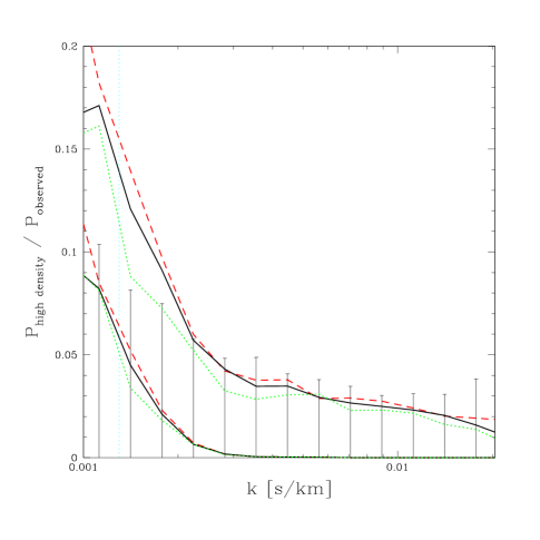
Figure 1: $P_{F}(k,z)$ from a random distribution of LLS and DLA (upper lines) or just DLA (lower lines), each with the observed column density distribution, relative to the observed Ly$\alpha$ forest $P_{F}(k,z)$ from (McDonald et al., 2004a). Red (dashed), black (solid), and green (dotted) lines show $z=2.2$, 3.2, and 4.2. The error bars indicate the fractional error on the observed $P_{F}(k,z)$ at $z=3.2$ (the errors at $z=2.2$ are very similar, while the errors at $z=4.2$ are $\sim 2$ times bigger). The vertical dotted line shows the largest scale used for constraining cosmology by (McDonald et al., 2004b).

We see that the effect is quite significant, and that more than half of it (on relevant scales) comes from the $\log(N)<20.3$ systems.

The region of a simulated spectrum that is being replaced by the high density system may be relevant, as we saw in the case with no damping wings, We include this effect using the lognormal model mock spectra described in McDonald et al. (2004a). These are not perfectly realistic, but they have the advantage over full numerical simulations that they can be of arbitrary length so the full extent of damping wings can be included. Figure 2 shows the power added to the mock spectra when high density systems with the observed column density distribution are added to the mock spectra, either at random locations, or using a mapping of the highest column density systems to the highest density maxima in the lognormal field.

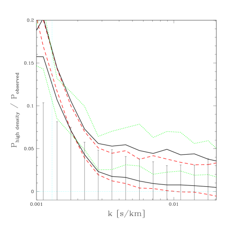
Figure 2: Change in $P_{F}(k,z)$ when LLS and DLA with the observed column density distribution are inserted into mock spectra of the Ly$\alpha$ forest, relative to the observed Ly$\alpha$ forest $P_{F}(k,z)$. The upper curves show the case where the high density systems are inserted randomly (different from Fig. 1 in that there was no background forest in that figure), while for the lower curves the LLS and DLA were inserted at the highest density maxima in the mock Ly$\alpha$ forest spectra. The line types and error bars are as in Fig. 1. Note that a consistent systematic error that is $1\sigma$ for any single point is very significant, because we have many $z$ and $k$ bins to average over.

We see that the location of the systems does matter. The change in high-$k$ power is removed when the systems are inserted at already high-density locations, presumably because this power is related to relatively low column density systems that are not significantly broadened by damping wings and thus produce absorption that is insensitive to column density, as seen above. In fact, the difference between the added power in the two cases is not significant to cosmological fits (McDonald et al., 2004b), apparently because the fractional effect is is relatively flat (i.e., $k$-independent) and thus mostly degenerate with $\bar{F}$ instead of the primordial power spectrum. The agreement in the McDonald et al. (2004b) fits between these two cases makes us confident that detailed, realistic simulations of high density systems will not produce a significantly different result. The primary effect comes simply from the self-correlation across the width of individual systems with damping wings, which is directly computable from the observed column density distribution.

How should we use these results to correct for their influence on the determination of the linear theory power spectrum, $P_{L}(k)$? The effect is essentially additive, so the form $P_{\rm theory}(k,z)=P_{\rm sim}(k,z)+P_{\rm damp}(k,z)$ is most natural, where $P_{\rm theory}(k,z)$ is the final prediction to be compared with observations, $P_{\rm sim}(k,z)$ is the prediction by simulations without damping wings, and $P_{\rm damp}(k,z)$ is the power shown in Figure 2. $P_{\rm damp}$ carries some uncertainty of course. As discussed in §2.1, the statistical errors on the number of LLSs and DLAs are probably about 15%, and the statistical error on $P_{\rm damp}$ should be proportional to this. However, because most observations do not distinguish column densities of LLSs, the important range of column densities just below the DLA cutoff is not directly constrained to the 15% level. For this reason, along with general caution to allow for any errors in our calculation, we suggest applying a 30% error to the amplitude of $P_{\rm damp}(k,z)$ in fits, i.e., adding $AP_{\rm damp}(k,z)$ to the simulated power, and $[(A-1)/0.3]^{2}$ to $\chi^{2}$. An even more cautious analysis might allow for redshift dependence of $A$; however, there is not any reason to think a break from the Zheng & Miralda-Escudé (2002) column density distribution template used in §2.1 should be significantly redshift dependent, and one might even argue that the constancy of the ratio of of $P_{\rm damp}(k,z)$ to $P_{\rm observed}(k,z)$ (Fig. 2) is unlikely to be a coincidence. McDonald et al. (2004b) find a value of $A=1.01\pm 0.24$, i.e., the power spectrum fit not only prefers our estimated amplitude, but is beginning to constrain the amplitude to better than our conservative 30% external constraint. One might think that a more careful study could reduce this error and thus reduce the errors on the final $P_{L}(k)$ measurement; however, McDonald et al. (2004b) shows that improving the error to 10% does not noticeably improve the $P_{L}(k)$ results (this may change as other parts of the $P_{L}(k)$ analysis are improved).

3 Fluctuations in the ionizing background

The two most recent studies of fluctuations in the ionizing background and their effect on the flux power spectrum are Meiksin & White (2004) and Croft (2003). The two differ in details: while Meiksin & White (2004) use an N-body (PM) simulation and are limited to small box sizes, Croft (2003) uses a larger $P^{3}M$ simulation and patches onto it sections of a high resolution hydrodynamic simulation. A large simulation box is needed to explore fluctuations in the ionizing background from quasars, whose typical separation is tens of megaparsecs. High resolution is needed to resolve the Ly$\alpha$ forest. Here we use a very large TPM simulation with 320$\,h^{-1}\,{\rm Mpc}$ box size and $1024^{3}$ resolution to obtain both a large box and a high resolution within the same simulation (Bode & Ostriker, 2003). This allows us to explore the background fluctuations on large scales and gives correct correlations between large and small scales. While the simulation does not converge in an absolute sense on small scales, it probably converges for the purpose of relative comparisons between simulation results with and without ionizing background fluctuations (Meiksin & White, 2004). The cosmological parameters of the simulation are $\Omega_{m}=0.3$, $H_{0}=70{\rm km/s/Mpc}$ and $\sigma_{8}=0.93$.

To generate a realization of the quasar background we first select the sites of quasar hosts. In Meiksin & White (2004) positions of these were chosen randomly, but this ignores the possibility that the Ly$\alpha$ forest and background fluctuations are correlated. In Croft (2003) quasar host sites were chosen based on overdensity criteria, because the resolution of the simulation was insufficient to resolve galactic size halos. We have actual halo catalogs from a halo finder, which are reliable down to masses around $10^{11}h^{-1}M_{\sun}$ (the particle mass is $3\times 10^{9}h^{-1}M_{\sun}$). We use these halos as potential quasar hosts. We assume all quasars have the same lifetime $t_{\rm QSO}$, which we will vary between $10^{7}-10^{8}$ years (Steidel et al., 2002).

We model the quasar luminosity function as a double power law,

$$\Phi(L)={\Phi^{*}\over(L/L_{*})^{\beta}+(L/L_{*})^{\beta_{2}}},$$ (2)

with the faint end slope $\beta_{2}=1.58$. For the bright end we explore two possibilities, $\beta=3.41$ as suggested by quasars with $z<2.3$ (Boyle et al., 2000), and $\beta=2.58$ found in high redshift quasars with $z>4$ (Fan et al., 2001). The latter choice is flatter, has more bright quasar sources and leads to stronger fluctuations. The B band magnitude corresponding to $L_{*}$ in equation 2 is assumed to be given by $M_{*}=-22.65-2.5(1.36z-0.27z^{2})$, while $\Phi_{*}=0.36\times 10^{-6}{\rm Mpc}^{-3}{\rm mag}^{-1}$ (Meiksin & White, 2003).

To generate a realization of quasars in the simulation at a given redshift we take the quasar luminosity function and multiply it by the ratio of the age of the universe at that redshift, $t_{\rm Hubble}$, to the quasar lifetime, $t_{\rm QSO}$. This gives us the density of quasar hosts, each of which will be a host to an active quasar at any time with a probability of $t_{\rm QSO}/t_{\rm Hubble}$. We then assign halo hosts to quasar hosts assuming a monotonic relation between the quasar luminosity (when active) and halo mass. We generate a turn-on time $t_{\rm on}$ for each quasar choosing randomly between 0 and $t_{\rm Hubble}$. In general we choose quasars down to $M_{B}=-22$, which is fainter than the turnover magnitude $M_{*}$.

To compute the background radiation at any given position we add up contributions from all quasars. We do this by first computing the time of observation $t_{\rm obs}$ for a given position along the line of sight. We compute the distance $r$ from that position to each quasar and convert it to light propagation time $t_{\rm prop}$. To count the contribution from a given quasar one must have $t_{\rm on}+t_{\rm prop}<t_{\rm obs}<t_{\rm on}+t_{\rm prop}+t_{\rm qso}$, so that the radiation from the quasar is passing through the given position at the time of observation. This procedure accounts for the light-cone effects discussed in Croft (2003).

Each quasar adds a contribution to the radiation field $\Gamma$ proportional to $L~{}r^{-2}\exp(-r/r_{\rm att})$. The attenuation length $r_{\rm att}$ is determined by the overall level of absorption of the radiation by neutral hydrogen. The actual value is somewhat uncertain and there are various estimates in the literature (Fardal & Shull, 1993; Haardt & Madau, 1996; Croft, 2003; Meiksin & White, 2004). For the low density Ly$\alpha$ forest simulations can be used. In addition there is also a significant contribution from high column density damped and Lyman-limit systems, which are typically not properly reproduced in simulations and their contribution has to be estimated separately. Here we will use $r_{\rm att}=1.7\times 10^{4}(1+z)^{-3.2}h^{-1}{\rm Mpc}$ (Meiksin & White, 2004), but we will also explore the more pessimistic scenario where the attenuation lengths are 50% shorter (at the lower limit of the various estimates in the literature). In general, shorter attenuation lengths lead to larger fluctuations, since nearby sources account for a larger fraction of the radiation in this case.

The attenuation length increases rapidly with decreasing redshift and at low redshifts it can exceed the simulation box size. This means that considering only the contributions from within the box will underestimate the background and so overestimate the fluctuations (since we always normalize the background relative to the required level needed to achieve a given mean level of absorption). We solve this by stacking together several boxes, summing over the quasars in all of them. These additional boxes are identical realizations of the central box and we use periodic boundary conditions to patch them together. In total we perform the summation over 27 boxes. Note that while the additional boxes are identical to the original box, the actual quasars contributing to a given position are not repeated, since the quasar lifetime is much shorter than the light travel time through the box and so no single quasar can contribute to a given point more than once. Examples of the radiation field along a line of sight are shown in figure 3, This example is for $z=3$, $t_{\rm QSO}=10^{8}$yr and $r_{\rm att}=161h^{-1}{\rm Mpc}$. We see that most lines of sight are very smooth with radiation density close to the mean, but every now and then the line of sight passes very close to an active quasar and the radiation density increases. In the most prominent cases one can see the light cone effects and times of quasar turn-on and turn-off.

Figure 3: Examples of radiation background fluctuations along a line of sight assuming all of the background comes from quasars. This example is for $z=3.29$ with $r_{\rm att}=161h^{-1}{\rm Mpc}$ and quasar lifetime $t=10^{8}$yr.

To generate Ly$\alpha$ forest spectra from a pure N-body simulation we choose a line of sight and use cloud-in-cell interpolation of the nearby particles onto a one dimensional grid consisting of 1024 cells of the same size as the original 3-d simulation cells. This gives us the density and velocity at each grid cell. We compute the neutral density/optical depth using the ionizing equilibrium relation

$$\tau=A{(1+\delta)^{1.7}\over\Gamma},$$ (3)

where $\delta$ is the dark matter overdensity, $\Gamma$ is the intensity of the radiation background, the factor of 1.7 is approximately valid for the observed temperature-density relation (for isothermal gas the slope is 2 and the results are almost identical), and $A$ is a constant of proportionality (Hui & Gnedin, 1997). For the ionizing background $\Gamma$ we take the local value at that position. We then map the neutral density field into redshift space by adding the peculiar velocity to the position at each grid cell and interpolate this field back to the grid. We ignore any additional thermal smoothing, since the grid cell size is already larger than the thermal broadening scale. Finally we compute the flux $F=\exp(-\tau)$. We vary the constant $A$ until achieving the desired mean flux decrement, $\bar{F}$, to match observations (see Meiksin & White (2004) for a recent compilation). Figure 4 shows the resulting power spectra as a function of redshift. Comparison to observations reveals good qualitative agreement over the whole range of scales and redshifts. When comparing the spectra with and without background radiation fluctuations we always match first the mean flux for the two cases.

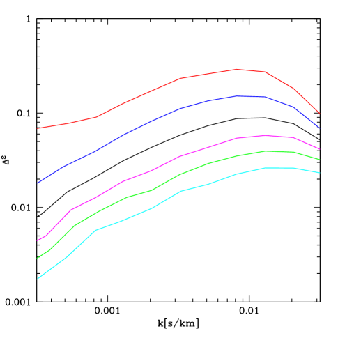
Figure 4: Flux power spectrum from the TPM simulation. The redshifts from top to bottom are $z=4.58$, 3.88, 3.29, 2.82, 2.40 and 2.05. The spectra agree qualitatively well with the observations.

For each line of sight we compute the flux distribution using the uniform background approximation and using the actual radiation field at each point. We then compute the power spectrum for each case, averaging over thousands lines of sight in each case. In figures 5 and 6 we present the results for these ratios for both $\beta=3.41$ and $\beta=2.58$. In all cases we show the scenario where the quasar contribution to the background is 100%. If quasars contribute a fraction $\alpha$, with the rest of the background uniform, then the effects in figures 5-6 are reduced roughly by this amount.

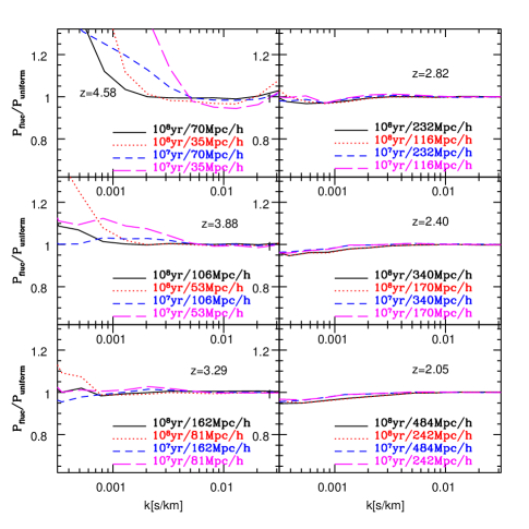
Figure 5: Ratio of the power spectra from simulations with ionizing background fluctuations versus uniform background, for various quasar lifetimes and attenuation lengths. This is for bright end slope of the quasar luminosity function $\beta=3.41$. We assume all of the ionizing background comes from quasars.

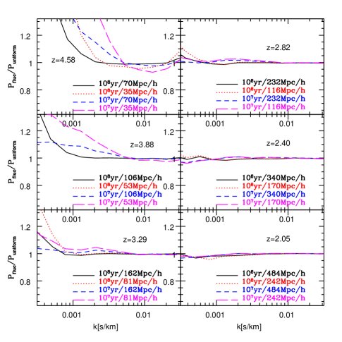
Figure 6: Same as figure 5 using bright end slope of the quasar luminosity function $\beta=2.58$.

There are several qualitative features in figures 5-6 worth pointing out. First is the fact that at high redshifts where the effect is significant the fluctuations in ionizing background enhance the power spectrum on large scales. A second important feature is the rapid decrease of the importance of fluctuations below $z=4$. This is a consequence of the increase in the attenuation length $r_{\rm att}$, which leads to more quasars contributing to a given position and thus reducing the fluctuations.

For the SDSS power spectrum measurements (McDonald et al., 2004a) the relevant range is $10^{-3}~{}{\rm s/km}<k<2\times 10^{-2}~{}{\rm s/km}$ and $2.2<z<4.2$. These observations do not go to sufficiently high redshift for these radiation background fluctuation effects to be clearly visible in the power spectra. There is no evidence for any enhancement of power on large scales at the highest redshifts ($z=4.2$); note, however, that the statistical errors are relatively large here (McDonald et al., 2004b). Some extreme models, like $t_{\rm QSO}=10^{7}$yr, $\beta=2.58$ and $r_{\rm att}=53h^{-1}$Mpc produce a 20% effect at $k=10^{-3}~{}{\rm s/km}$ and $z=3.88$. These models are strongly disfavored by the data. Other models, like $t_{\rm QSO}=10^{8}$yr, $\beta=3.4$ and $r_{\rm att}=106h^{-1}$Mpc, produce no effect at this redshift and are acceptable even if quasars dominate the background radiation field. The effects are even smaller at lower redshift.

Comparing our results to Croft (2003) at $z=3$, we note that the effect found there is somewhat larger and has the opposite sign. It is unclear what the source of the difference is, but one possibility is the hybrid hydrodynamic-dark matter approach used in Croft (2003), which allows for only a qualitative estimate of the effect. Another difference in the two treatments is the choice of quasar hosts. While we use actual halos, overdensities were used in Croft (2003). Finally there are also some differences in the adopted quasar luminosity function. While redshift dependence was not explored in Croft (2003), our analysis suggests that a model that produces a 20% effect at $k=10^{-3}~{}{\rm s/km}$ and $z=3$ will lead to a large effect at $z=4$ and will be excluded by the absence of any such effect in real data (McDonald et al., 2004a).

There could be additional sources of ionizing radiation such as Lyman break galaxies (Steidel et al., 2003) or reradiation of photons from the absorbing sources in the forest (Haardt & Madau, 1996). It is often assumed that due to their higher density these sources lead to uniform radiation field and so their effects on ionizing fluctuations need not be considered. However, these sources can still be clustered and if the large scale effects are coherent their contribution could be important. Here we address this by choosing all halos with masses between $10^{11}h^{-1}M_{\sun}$ and $10^{12}h^{-1}M_{\sun}$ as the hosts of LBGs. Their number density is $6\times 10^{-3}h^{3}{\rm Mpc}^{-3}$, comparable or somewhat larger than the density of known LBGs (Steidel et al., 2003). We assign a luminosity proportional to halo mass and assume long lifetimes, comparable to the Hubble time at a given redshift. This model need not be correct, since LBGs could be starburst galaxies hosted by small halos rather than sitting in the most massive halos at that redshift (Somerville et al., 2001), but we lack mass resolution to resolve these small halos and test this alternative model. It is likely that the starburst model leads to more homogeneous radiation background.

The rest of the model is the same as for quasars and in our calculations we assume all of ionizing background comes from these sources. In figure 7 we show the effect on the flux power spectrum as a function of redshift. We see that the redshift dependence is still present, but is weaker than for quasars. The effect is small except on largest scales, where it can reach 10% at redshifts of interest. Interestingly, over the relevant range of scales the effect leads to a suppression of power, contrary to the quasar case. This could be a consequence of coherence between the galaxy field and Ly$\alpha$ forest  which comes into better light for these high density sources, unlike the case of quasars where shot noise was more important.

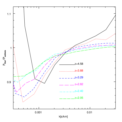
Figure 7: Example of the effect on the flux power spectrum if the sources of ionizing radiation are galaxies with density comparable to that of LBGs. We find a suppression of power in this case.

In an actual analysis of the real data (McDonald et al., 2004b) we tried adopting the templates of the worst case quasar scenario and allowing the fractional quasar contribution to vary smoothly with redshift (while the estimates of quasar contribution to the total background are uncertain, we do not expect the relative fraction to vary wildly with redshift (Meiksin & White, 2003)). The data strongly disfavor these models (McDonald et al., 2004b). This could be because the worst case scenario quasar model adopted is too extreme, so other models in figures 5-6 could still be acceptable as they have little or no effect on the flux power spectrum. Alternatively, the quasar effect should be combined with the contribution from galaxies, which leads to an opposite effect and so the two contributions partially cancel out.

4 Galactic superwinds

The effects of GSW on the Ly$\alpha$ forest power spectrum have been explored before (Croft et al., 2002a; Desjacques et al., 2003), where the wind simulation power spectra were compared to those with no winds. In this paper we perform a similar analysis using hydrodynamic simulations with and without GSW, but we also account for the allowed changes in the mean absorption, temperature-density relation, and filtering length. These are part of our standard Ly$\alpha$ forest analysis (McDonald et al., 2004b) and our goal is to investigate whether there are additional effects that go beyond the simple changes in the mean transmitted flux fraction, $\bar{F}$, mean temperature, $T_{0}$, slope of the temperature-density relation, $\gamma-1$, and filtering length, $k_{F}$.

Our simulations (similar, but not the same as those in §2.2) are based on a fixed grid Eulerian cosmological hydrodynamic code with a TVD shock-capturing scheme (Cen et al., 2004). They include the effects of cooling, heating, star formation, and supernova (SN) feedback. The cosmology adopted here is standard $\Lambda$CDM with $\Omega_{m}=0.29$, $\Omega_{b}=0.047$, $H_{0}=70{\rm km/s/Mpc}$, and $\sigma_{8}=0.85$. All of the simulations used here have a box size of $11h^{-1}$Mpc in comoving units, $216^{3}$ dark matter particles, and gas followed on a $432^{3}$ grid. See Cen et al. (2004) for additional simulations and resolution tests.

As described in Cen et al. (2004), there is no attempt to model the subgrid physics in these simulations, which would in principle determine how much of the SN energy is injected into the galaxies and how much of it can escape them. Instead it is assumed the wind energy (and mass) flux is proportional to the star formation rate $\dot{M}_{*}$ and the proportionality constant is calibrated on observations (Heckman, 2003; Pettini et al., 2001). For energy output this implies $\dot{E}_{GSW}=e_{GSW}c^{2}\dot{M}_{*}$ with $e_{GSW}=3\times 10^{-6}$. We assume a similar relation for the mass output. These are somewhat uncertain and we want to explore worst case scenarios, so we will analyze simulations where the outflow energy is increased by 5 to $e_{GSW}=1.5\times 10^{-5}$.

As discussed in Cen et al. (2004), the wind simulations produce significant outflows which can heat up the IGM and pollute it with metals at a level consistent with observations. However, they appear to have little effect on the distribution of neutral hydrogen. This is because GSW propagate preferentially in the directions of low density, so while they heat up the gas in voids, they do not affect the structure in higher density regions where most of the fluctuations in absorption by neutral hydrogen are produced (Theuns et al., 2002).

To quantify these statements we explore explicitly the effect of GSW on the Ly$\alpha$ forest flux power spectrum. This is shown in figure 8 for the more extreme value $e_{GSW}=1.5\times 10^{-5}$ at 3 different redshifts. We do not show the results for the more realistic value $e_{GSW}=3\times 10^{-6}$ since the effects there are less significant. While we see that the effects for this more extreme case can be up to 10% over the range of observational interest, especially at $z=3$, the effect is mostly due to the fact that the IGM temperature history and density dependence have changed. Without winds, the temperature parameters at $z=$(2, 3, 4) are $T_{1.4}=$(21699, 17680, 13478) K and $\gamma-1=$(0.454, 0.397, 0.497), while with maximum winds, they change to $T_{1.4}=$(19563, 15012, 14455) K and $\gamma-1=$(0.479, 0.493, 0.477), where $T_{1.4}$ is the temperature at density 1.4 times the mean.

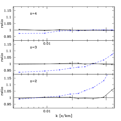
Figure 8: Ratio of the power spectra between strong wind simulation and no wind simulation for $z=2,3,4$. Dashed line shows direct comparison, solid line the comparison after adjusting $\bar{F}$, the temperature-density relation, and the filtering scale.

To explore the effect of changes in the temperature-density relation, we recompute the power spectra after modifying the temperatures in the simulations to impose different $T_{1.4}$ and $\gamma-1$. We do this in the following way: First we verify that computing the neutral hydrogen density from the gas density using the ionizing equilibrium assumption leads to identical results as the simulation outputs themselves. Then we compute $T_{1.4}$ and $\gamma-1$ for a simulation using a least absolute deviation fit (Press et al., 1992) to all the points in the simulation with $1<\rho/\bar{\rho}<2$. This fit effectively uses the median rather than the mean temperature, which is desirable because the mean temperature values are heavily biased by rare regions with extremely high temperatures in simulations with GSW. For each gas cell we compute from its density the expected temperature for the original temperature-density relation in the simulation and for a modified temperature-density relation. We take the ratio between the two and multiply the actual value of the temperature in the cell by it, therefore preserving the scatter in the temperature-density relation present in the hydrodynamic simulation. We then use the new temperatures to compute the neutral density using the ionizing equilibrium equation, and finally recompute the flux power spectrum.

To see how much of the difference between simulations with and without winds is accounted for by simple temperature-density relation changes, we recompute the power spectra in the simulations with GSW for a variety of modified temperature-density relations until we find one that matches best the power spectrum of the simulation without GSW. We find that the required changes in $T_{1.4}$ and $\gamma-1$ are in similar to the changes in the median-fitted values, but we did not restrict ourself to these in our analysis since it is not clear that they are the appropriate averages. For the purpose of the power spectrum analysis, finding the values that minimize the power spectrum differences is most relevant, since in our power spectrum analysis we always marginalize over $T_{1.4}$ and $\gamma-1$.

While we find good agreement between $P_{F}$ in wind and no-wind simulations using this procedure where we only modify $T_{1.4}$ and $\gamma-1$, we can improve it further by noting that a change in the temperatures also changes the filtering length $k_{F}$. This filtering length depends on the full temperature history of the IGM from reionization onwards. We do not try to make analytic predictions of what the filtering length should be given the temperature history of the IGM due to the difficulties in interpreting the scatter in temperature at a given density. Instead we follow the procedure in McDonald et al. (2004b), using hydro-PM simulations (Gnedin & Hui, 1998) to find the effect of changing the reionization redshift. We apply the change that minimizes the residual effect of the winds when combined with changes in $T_{1.4}$ and $\gamma-1$. Finally, we also allow small adjustments in the mean absorption level, $\bar{F}$, which must be marginalized over in any cosmological fit. The final result is shown in figure 8, where we see that using the freedom of varying $\bar{F}$, $T_{1.4}$, $\gamma-1$, and $k_{F}$ cancels completely the effect of GSW in the simulations over the region of observational interest.

The parameter variations we used to produce this agreement are not extreme. Beyond the change in median temperature-density relation estimated directly from the simulations, the modifications needed are as follows: We modified the filtering ($k_{F}$) effect by 20% of the difference between two cases: the case when reionization heats the gas to 25000 K at $z=7$ and the case when reionization heats the gas to 50000 K at $z=17$ (we present the change this way because we interpolated between these two models instead of actually running intermediate simulations (McDonald et al., 2004b)). Note that we do not adjust $k_{F}$ independently at each redshift – the early-time thermal history is modified and this effects each of the redshifts we show in a self-consistent way. At $z=2$, we make the additional small modifications $\Delta\bar{F}=-0.001$, $\Delta T_{1.4}=-800$ K, and $\Delta\gamma-1=-0.03$; at $z=3$, we make the modifications $\Delta\bar{F}=+0.006$, $\Delta T_{1.4}=-1000$ K, and $\Delta\gamma-1=-0.01$; and finally, at $z=4$, we make the changes $\Delta\bar{F}=+0.0065$, $\Delta T_{1.4}=+1000$ K, and $\Delta\gamma-1=0.05$. All of these changes are small relative to the uncertainty in our measurements of these parameters (McDonald et al., 2004b).

While the simulation box is too small to be able to probe larger scales, the flatness of the final result on large scales suggests that these effects are only important on small scales and that these conclusions are unlikely to be modified if larger simulation boxes were used. Note that we find no effect both in the simulation with the expected GSW amplitude, as well as in the one where it was increased by a factor of 5. We only show the worse case scenario in figure 8.

While these results are comforting, they should not be viewed as a conclusive proof that GSW have no effect on Ly$\alpha$ forest flux power spectrum. For one thing, it is not clear that our simulations fare any better than other simulations in explaining the flux enhancement observed in lines of sight very close to LBGs (Adelberger et al., 2003). While no realistic simulations to date have been able to reproduce this result entirely, it is possible that it is a consequence of a statistical fluctuation, hosts of LBGs being less massive than usually assumed, galaxy proximity effect, selection effects, or any combination of these. Moreover, the fact that Desjacques et al. (2003) come close to explaining these observations without affecting the flux power spectrum is comforting. However, it is also possible that we are still missing some essential physics and that the winds are much more destructive of the IGM, although there are additional constraints on this like the flux probability distribution statistics (McDonald et al., 2000). Even in such a case it is not clear how much of the effect is degenerate with the parameters we already marginalized over, such as $\bar{F}$, $T_{1.4}$, $\gamma-1$, and $k_{F}$. It is clear that more work is needed to exclude all possible sources of contamination of the Ly$\alpha$ forest flux power spectrum, even if the current modeling suggests that GSW are not problematic.

5 Conclusions

In this paper we have analyzed physical effects on the power spectrum of the Ly$\alpha$ forest. We focus on effects that would not otherwise be part of the standard simulation-based analysis (McDonald et al., 2004b). In section 2 we analyze the contribution from high density systems, especially those with damping wings, which are not simulated properly in the current generation of simulations. We show that their inclusion adds power on large scales and accounting for this leads to an increase in the deduced slope of primordial fluctuations (McDonald et al., 2004b). The amplitude of the effect can be estimated both from direct counting of these high density systems as well as using the templates in the power spectrum analysis itself, taking advantage of their specific form as a function of scale and redshift. At the moment the uncertainties in the former make the latter approach competitive or even better (McDonald et al., 2004b), suggesting that a better determination of the high density systems as a function of column density and redshift would be useful for accurate determination of this effect. But even within the current uncertainties it is clear that the effect is appreciable compared to the size of the statistical error given by the new data.

In section 3 we analyze the effects of fluctuations in the ionizing background. We focus on quasars, which are believed to be the dominant source of ionizing background at these redshifts. These fluctuations lead to an enhancement of power on large scales which rapidly increases with redshift, because the photon attenuation length is significantly shorter at higher redshifts. This allows us to develop templates that can be used to identify the effect in the real data. The SDSS data show no evidence of this effect (McDonald et al., 2004b). We also investigated a simple example that could correspond to galactic sources of radiation, matching the density of LBG galaxies. Contrary to naive expectations we do not find that this more dense population of sources leads to a more homogeneous ionizing background, likely as a result of clustering of sources. The coherent nature of these sources and Ly$\alpha$ forest leads to a suppression of power on large scales. The effect is relatively small on scales probed by SDSS and is somewhat redshift dependent, which allows it to be constrained from the data.

We should caution that the current level of modeling remains rather simplistic and there are many possible scenarios we did not explore, so we cannot conclusively rule out that fluctuations in ionizing background are unimportant for the flux power spectrum statistics. To put things into perspective we note that the effect of damped systems, which is 20% at $k\sim 10^{-3}{\rm s/km}$ (figure 2), results in a 0.06 change in the slope of the power spectrum, which is slightly more than 1-$\sigma$ (McDonald et al., 2004b). In comparison to this the effects from ionizing fluctuations are below 10% at $k\sim 10^{-3}{\rm s/km}$. Thus these effects are unlikely to change the estimate of the slope by more than 1-$\sigma$ given the current uncertainties. In addition, they have stronger redshift dependence than damped systems, which makes it possible to identify and remove them. It is however important to understand them better if we want to extract all of the information present in the SDSS data, as the current constraints on the slope are limited by theoretical modeling uncertainties and could be improved further.

In contrast to the effects of damped systems and ionizing background fluctuations, which mostly change the power spectrum on large scales, galactic superwinds are predominantly affecting small scales, where several other parameters are also important. In section 4 we have shown that galactic superwinds used in our simulations do not affect the Ly$\alpha$ forest flux power spectrum statistics after marginalization over the mean absorption level, temperature-density relation of the IGM, and its filtering scale. This is true even though the same GSW can heat up a significant fraction of the volume and pollute the IGM with metals at a level consistent with observations (Cen et al., 2004). This again is not a conclusive proof that winds are unimportant and there could still be physics missing in these simulations, but a definitive answer can only come by investigating it in simulations which are sufficiently realistic and are able to satisfy all of the observational constraints.

In summary, current models suggest that various physical effects analyzed in this paper, which are not part of the current simulations, are not destructive for the power spectrum statistics, even if they may weaken its predictive power. This conclusion is preliminary and more work is needed to investigate these and other effects before their impact is fully understood and corrected for in the analysis. One of the effects we did not investigate here are fluctuations in the IGM temperature, which could be caused by patchy helium reionization at these redshifts (Zaldarriaga, 2002). This is unlikely to be a major effect, since temperature has only a minor effect on the flux power spectrum statistics on large scales probed by SDSS, but this should be verified with explicit calculations. Progress on these issues will come from both theoretical and observational directions. Better theoretical modeling of the effects discussed in this paper, with simulations that include more realistic physics, will allow a better assessment of their impact. Improvements in observational tests of the Ly$\alpha$ forest will be equally important. A few examples of these that go beyond the flux power spectrum are of abundances of damped systems, correlations between Ly$\alpha$ forest and quasars or galaxies and higher order correlations of Ly$\alpha$ forest  such as the bispectrum analysis or one-point distribution of the flux. All of these will allow to better constrain the contribution of these effects to the flux power spectrum and determine their effect on the cosmological constraints derived from Ly$\alpha$ forest .

We thank Zheng Zheng for providing the column density distribution templates, and Jason Prochaska for the tables of DLA data. We thank Joop Schaye for helpful discussions. Some of the computations used facilities at Princeton provided in part by NSF grant AST-0216105, and some computations were performed at NCSA. US is supported by a fellowship from the David and Lucile Packard Foundation, NASA grants NAG5-1993, NASA NAG5-11489 and NSF grant CAREER-0132953. RC acknowledges grants AST-0206299 and NAG5-13381.

References

- Adelberger et al. (2003) Adelberger K. L., Steidel C. C., Shapley A. E., Pettini M., 2003, ApJ, 584, 45
- Aracil et al. (2004) Aracil B., Petitjean P., Pichon C., Bergeron J., 2004, A&A, 419, 811
- Bode & Ostriker (2003) Bode P., Ostriker J. P., 2003, ApJS, 145, 1
- Boyle et al. (2000) Boyle B. J., Shanks T., Croom S. M., Smith R. J., Miller L., Loaring N., Heymans C., 2000, MNRAS, 317, 1014
- Bruscoli et al. (2003) Bruscoli M., Ferrara A., Marri S., Schneider R., Maselli A., Rollinde E., Aracil B., 2003, MNRAS, 343, L41
- Cen et al. (2004) Cen R., Nagamine K., Ostriker J. P., 2004, ArXiv Astrophysics e-prints, astro-ph/0407143
- Cen et al. (2003) Cen R., Ostriker J. P., Prochaska J. X., Wolfe A. M., 2003, ApJ, 598, 741
- Croft (2003) Croft R. A. C., 2003, ArXiv Astrophysics e-prints, astro-ph/0310890
- Croft et al. (2002a) Croft R. A. C., Hernquist L., Springel V., Westover M., White M., 2002a, ApJ, 580, 634
- Croft et al. (2002b) Croft R. A. C., Weinberg D. H., Bolte M., Burles S., Hernquist L., Katz N., Kirkman D., Tytler D., 2002b, ApJ, 581, 20
- Croft et al. (1998) Croft R. A. C., Weinberg D. H., Katz N., Hernquist L., 1998, ApJ, 495, 44
- Croft et al. (1999) Croft R. A. C., Weinberg D. H., Pettini M., Hernquist L., Katz N., 1999, ApJ, 520, 1
- Desjacques et al. (2003) Desjacques V., Nusser A., Haehnelt M. G., Stoehr F., 2003, ArXiv Astrophysics e-prints, astro-ph/0311209
- Fan et al. (2001) Fan X. et al., 2001, AJ, 121, 54
- Fardal & Shull (1993) Fardal M. A., Shull J. M., 1993, ApJ, 415, 524
- Gardner et al. (2001) Gardner J. P., Katz N., Hernquist L., Weinberg D. H., 2001, ApJ, 559, 131
- Gnedin & Hamilton (2002) Gnedin N. Y., Hamilton A. J. S., 2002, MNRAS, 334, 107
- Gnedin & Hui (1998) Gnedin N. Y., Hui L., 1998, MNRAS, 296, 44
- Haardt & Madau (1996) Haardt F., Madau P., 1996, ApJ, 461, 20
- Heckman (2003) Heckman T. M., 2003, in Revista Mexicana de Astronomia y Astrofisica Conference Series
- Hui & Gnedin (1997) Hui L., Gnedin N. Y., 1997, MNRAS, 292, 27
- Kim et al. (2003) Kim T. ., Viel M., Haehnelt M. G., Carswell R. F., Cristiani S., 2003
- Kollmeier et al. (2003) Kollmeier J. A., Weinberg D. H., Davé R., Katz N., 2003, ApJ, 594, 75
- Maselli et al. (2004) Maselli A., Ferrara A., Bruscoli M., Marri S., Schneider R., 2004, MNRAS, 350, L21
- McDonald et al. (2002) McDonald P., Miralda-Escudé J., Cen R., 2002, ApJ, 580, 42
- McDonald et al. (2000) McDonald P., Miralda-Escudé J., Rauch M., Sargent W. L. W., Barlow T. A., Cen R., Ostriker J. P., 2000, ApJ, 543, 1
- McDonald et al. (2004a) McDonald P. et al., 2004a, ArXiv Astrophysics e-prints, astro-ph/0405013
- McDonald et al. (2004b) McDonald P., Seljak U., Cen R., the SDSS Collaboration , 2004b, astro-ph/0407377
- Meiksin & White (2001) Meiksin A., White M., 2001, MNRAS, 324, 141
- Meiksin & White (2003) Meiksin A., White M., 2003, MNRAS, 342, 1205
- Meiksin & White (2004) Meiksin A., White M., 2004, MNRAS, 350, 1107
- Miralda-Escude et al. (1996) Miralda-Escude J., Cen R., Ostriker J. P., Rauch M., 1996, ApJ, 471, 582
- Nagamine et al. (2004) Nagamine K., Springel V., Hernquist L., 2004, MNRAS, 348, 421
- Péroux et al. (2003a) Péroux C., Dessauges-Zavadsky M., D’Odorico S., Kim T., McMahon R. G., 2003a, MNRAS, 345, 480
- Péroux et al. (2003b) Péroux C., McMahon R. G., Storrie-Lombardi L. J., Irwin M. J., 2003b, MNRAS, 346, 1103
- Pettini et al. (2001) Pettini M., Shapley A. E., Steidel C. C., Cuby J., Dickinson M., Moorwood A. F. M., Adelberger K. L., Giavalisco M., 2001, ApJ, 554, 981
- Press et al. (1992) Press W. H., Teukolsky S. A., Vetterling W. T., Flannery B. P., 1992, Numerical recipes in C. The art of scientific computing. Cambridge: University Press, —c1992, 2nd ed.
- Prochaska & Herbert-Fort (2004) Prochaska J. X., Herbert-Fort S., 2004, ArXiv Astrophysics e-prints, astro-ph/0403391
- Schaye (2001) Schaye J., 2001, ApJ, 559, 507
- Schaye et al. (2003) Schaye J., Aguirre A., Kim T., Theuns T., Rauch M., Sargent W. L. W., 2003, ApJ, 596, 768
- Smith et al. (1986) Smith H. E., Cohen R. D., Bradley S. E., 1986, ApJ, 310, 583
- Somerville et al. (2001) Somerville R. S., Primack J. R., Faber S. M., 2001, MNRAS, 320, 504
- Songaila & Cowie (1996) Songaila A., Cowie L. L., 1996, AJ, 112, 335
- Steidel et al. (2003) Steidel C. C., Adelberger K. L., Shapley A. E., Pettini M., Dickinson M., Giavalisco M., 2003, ApJ, 592, 728
- Steidel et al. (2002) Steidel C. C., Hunt M. P., Shapley A. E., Adelberger K. L., Pettini M., Dickinson M., Giavalisco M., 2002, ApJ, 576, 653
- Theuns et al. (2002) Theuns T., Viel M., Kay S., Schaye J., Carswell R. F., Tzanavaris P., 2002, ApJ, 578, L5
- Viel et al. (2004) Viel M., Haehnelt M. G., Carswell R. F., Kim T.-S., 2004, MNRAS, 349, L33
- Wolfe et al. (1986) Wolfe A. M., Turnshek D. A., Smith H. E., Cohen R. D., 1986, ApJS, 61, 249
- Zaldarriaga (2002) Zaldarriaga M., 2002, ApJ, 564, 153
- Zheng & Miralda-Escudé (2002) Zheng Z., Miralda-Escudé J., 2002, ApJ, 568, L71
- Zuo (1992) Zuo L., 1992, MNRAS, 258, 36