The Linear Theory Power Spectrum from the Lyman-$\alpha$ Forest in the Sloan Digital Sky Survey

Abstract

We analyze the SDSS Ly$\alpha$ forest $P_{F}(k,z)$ measurement to determine the linear theory power spectrum. Our analysis is based on fully hydrodynamic simulations, extended using hydro-PM simulations. We account for the effect of absorbers with damping wings, which leads to an increase in the slope of the linear power spectrum. We break the degeneracy between the mean level of absorption and the linear power spectrum without significant use of external constraints. We infer linear theory power spectrum amplitude $\Delta^{2}_{L}(k_{p}=0.009~{}{\rm s/km},z_{p}=3.0)=0.452_{-0.057~{}-0.116}^{+0.069~{}+0.141}$ and slope $n_{\rm eff}(k_{p},z_{p})=-2.321_{-0.047~{}-0.102}^{+0.055~{}+0.131}$ (possible systematic errors are included through nuisance parameters in the fit — a factor $\gtrsim 5$ smaller errors would be obtained on both parameters if we ignored modeling uncertainties). The errors are correlated and not perfectly Gaussian, so we provide a $\chi^{2}$ table to accurately describe the results. The result corresponds to $\sigma_{8}=0.85$, $n=0.94$, for a $\Lambda$CDM model with $\Omega_{m}=0.3$, $\Omega_{b}=0.04$, and $h=0.7$, but is most useful in a combined fit with the CMB. The inferred curvature of the linear power spectrum and the evolution of its amplitude and slope with redshift are consistent with expectations for $\Lambda$CDM models, with the evolution of the slope, in particular, being tightly constrained. We use this information to constrain systematic contamination, e.g., fluctuations in the UV background. This paper should serve as a starting point for more work to refine the analysis, including technical improvements such as increasing the size and number of the hydrodynamic simulations, and improvements in the treatment of the various forms of feedback from galaxies and quasars.

1 Introduction

While the Ly$\alpha$ forest was discovered long ago (Lynds, 1971), a clear physical picture was not settled on until relatively recently. Observations of absorption in pairs of spectra showing coherence of Ly$\alpha$ forest absorption over hundreds of kpc (Bechtold et al., 1994; Dinshaw et al., 1994) demonstrated the key result that came from numerical simulations of the intergalactic medium (IGM), that the absorption features arose in low density structures that must contain a large fraction of the baryons and merge continuously with the background, instead of being dense, discrete systems. This was confirmed when the Keck HIRES spectrograph (Vogt et al., 1994) produced fully resolved spectra that were qualitatively explained by hydrodynamic simulations and semi-analytic models (Bi et al., 1992; Cen et al., 1994; Zhang et al., 1995; Hernquist et al., 1996; Miralda-Escude et al., 1996; Hui & Gnedin, 1997; Dave et al., 1997; Theuns et al., 1998; Gnedin & Hui, 1998). The Ly$\alpha$ forest absorption appears to arise from continuously fluctuating photoionized gas in the IGM, with density near the universal mean and temperatures around $10^{4}$ K. The structure of the absorption field can be derived from the primordial density field with reasonable accuracy using numerical simulations, smoothed on scales smaller than a few hundred comoving $\,h^{-1}\,{\rm kpc}$ by gas pressure and thermal broadening in redshift space.

Starting with Croft et al. (1998), the statistic of choice for comparing observations of the Ly$\alpha$ forest to predictions of different cosmologies has been the power spectrum, $P_{F}(k,z)$, of the transmitted flux fraction, $F(\lambda)=\exp[-\tau(\lambda)]$. Observational measurements of $P_{F}(k,z)$ have been presented in several recent papers (Croft et al., 1998; McDonald et al., 2000; Croft et al., 2002; Kim et al., 2004b, a; McDonald et al., 2004). In parallel with the observational efforts there has been considerable effort to interpret these measurements using numerical simulations (Croft et al., 1998; McDonald et al., 2000; Zaldarriaga et al., 2001; Croft et al., 2002; Gnedin & Hamilton, 2002; Zaldarriaga et al., 2003; Seljak et al., 2003; Viel et al., 2004). Other statistics of the fluctuations in transmitted flux are also useful, with recent papers studying the bispectrum (Mandelbaum et al., 2003; Viel et al., 2004b; Fang & White, 2004) and very large scale fluctuations (Tytler et al., 2004).

In the standard picture of the Ly-$\alpha$ forest the gas in the IGM is in ionization equilibrium. The rate of ionization by the UV background balances the rate of recombination of protons and electrons. The recombination rate depends on the temperature of the gas, which is a function of the gas density. The temperature-density relation can be parameterized by an amplitude, $T_{0}$, and a slope $\gamma-1=d\ln T/d\ln\rho$. The uncertainties in the intensity of the UV background, the mean baryon density, and other parameters that set the normalization of the relation between optical depth and density can be combined into one parameter: the mean transmitted flux, $\bar{F}$. We always treat $T_{1.4}$ (we follow McDonald et al. (2001) in specifying the temperature-density relation at density 1.4 times the mean), $\gamma-1$, and $\bar{F}$ as the independent (adjustable) variables in our analysis. For example, when we perform a convergence test comparing two simulations with different resolution we compare at fixed $\bar{F}$, even though this may require us to use different strengths of the ionizing background when constructing the simulated spectra.

In general the flux power spectrum, $P_{F}(k,z)$, is a function of the linear matter power spectrum, $P_{L}(k)$, cosmological parameters such as the matter density, $\Omega_{m}$, which we denote collectively as $\mathbf{p}_{\rm cosmology}$, and parameters of the Ly$\alpha$ forest model, which we denote as $\mathbf{p}_{\rm forest}$ (parameters in addition to $T_{1.4}$, $\gamma-1$, and $\bar{F}$ are introduced later). In observationally favored $\Lambda$CDM models the universe is Einstein-de Sitter at $z>2$, so if velocity units are used for $k$ we can drop the dependence on cosmological parameters, which determine the relation between velocity and comoving coordinates. (This relation must of course be reinstated when comparisons to explicit cosmological models are performed, but this is not a subject of this paper.)

We do not attempt to invert the flux power spectrum to a band-power description of $P_{L}(k)$. The linear power spectrum $P_{L}(k^{\prime})$ contributes to $P_{F}(k)$ at all $k$ (we use $k^{\prime}$ and $k$ here to make it clear that the two are not fundamentally connected), and the transformation is generally nonlinear. As a result inversion requires a large number of simulations in which the power in the bands is varied, in principle in combination and by varying amounts. This does not mean that such an inversion is impossible, but simple attempts we tried to devise have failed and current inversion treatments that exist in the literature are not sufficiently reliable for this purpose (Zaldarriaga et al., 2003; Seljak et al., 2003).

Instead we parametrize the information we wish to extract in terms of $\Delta^{2}_{L}(k,z)\equiv k^{3}P_{L}(k,z)/2\pi^{2}$, $n_{\rm eff}(k,z)\equiv d\ln P_{L}/d\ln k$, and $\alpha_{\rm eff}(k,z)\equiv dn_{\rm eff}/d\ln k$, the amplitude, logarithmic slope, and curvature of $P_{L}$, all evaluated at a pivot redshift $z_{p}$ and pivot wavenumber $k_{p}$, at which the information is near maximum. We adjust these variables in simulations, covering a broad range of values to obtain predictions of the flux power spectrum over the whole range of interest.

Our analysis is based on the $P_{F}(k,z)$ measurement of McDonald et al. (2004), which used 3300 Sloan Digital Sky Survey spectra from data releases one and two (Fukugita et al., 1996; Gunn et al., 1998; York et al., 2000; Hogg et al., 2001; Stoughton et al., 2002; Smith et al., 2002; Richards et al., 2002; Pier et al., 2003; Blanton et al., 2003; Abazajian et al., 2003, 2004). The SDSS sample is nearly two orders of magnitude larger than the samples available previously. Because the spectra are of lower resolution than HIRES spectra the small scale information is erased, so we supplement our study with the HIRES-based $P_{F}(k,z)$ measurement of McDonald et al. (2000). We do not include in our standard analysis the more recent measurements by Croft et al. (2002) and Kim et al. (2004b, a), because these show signs of a systematic discrepancy and/or underestimation of errors when compared to SDSS Ly$\alpha$ forest data (McDonald et al., 2004); however, we do present an alternative analysis using these results with some allowance for systematic errors, which gives results consistent with our standard analysis.

This paper is part of a closely intertwined set of four papers, including McDonald et al. (2004), McDonald et al. (2005), and Seljak et al. (2005). The observational measurement of $P_{F}(k,z)$ was presented in McDonald et al. (2004), which stands alone independent of theory, and makes a strong case that the systematic errors in the measured flux power spectrum are for practical purposes smaller than the statistical errors. The present paper transforms the flux power spectrum measurement into a constraint on the amplitude, slope, and curvature of the linear theory matter power spectrum at z=3 and comoving scale of a few Mpc. This constraint should apply to a wide range of cosmological models with linear power spectra similar to those favored by current observations, though it should not be applied to models with sharp breaks in the power spectrum on the scales of the measurement or to warm dark matter models (see more discussion below). For this class of models, we believe that the systematic errors in our inferred linear $P(k)$ constraints are also below the statistical errors (after several effects that would otherwise lead to systematic errors are included in the fit through nuisance parameters), though more testing with hydrodynamic simulations is desirable as discussed below. The results of this paper allow the SDSS flux power spectrum measurement to be incorporated in a straightforward way into cosmological parameter constraints drawing on multiple cosmological observables. We defer this task to a separate paper, Seljak et al. (2005), since it requires discussion of the other data sets to be used and the methodology for combining them. However, we note that the additional leverage provided by the Ly$\alpha$ forest power spectrum at small scales allows much improved constraints on the inflationary spectral index, $n$, the running of that index with scale, and neutrino masses. Also, some of the details on how we treat high column density systems and UV background fluctuations, and an investigation of galactic winds are described in another paper, McDonald et al. (2005).

The layout of this paper is as follows: Section 2 gives a detailed description of how we make our prediction of $P_{F}(k,z)$ given $P_{L}(k)$, $\mathbf{p}_{\rm cosmology}$, and $\mathbf{p}_{\rm forest}$. Section 3 describes how we perform $\chi^{2}$ fits to the observations to estimate $\Delta_{L}^{2}(k_{p},z_{p})$ and $n_{\rm eff}(k_{p},z_{p})$ and their errors. Finally, §4 contains our conclusions.

2 Numerical Simulations of $P_{F}(k,z)$

In this section we explain how we translate any given set of model parameters into a prediction of $P_{F}(k,z)$. We assume that any winds from galaxies do not effect $P_{F}(k,z)$ beyond the modest effect of the local energy injection in our hydrodynamic simulations (we do allow for some uncertainty in this effect by marginalizing over the differences between three versions of the feedback in the simulations). Winds are explored in more detail in a companion paper (McDonald et al., 2005). We also assume that the density-temperature-neutral density relation is not made inhomogeneous by inhomogeneous reionization and heating (i.e., patchy reionization of either hydrogen or helium). We expect to investigate these issues in the future.

2.1 Background

In the redshift range of interest, $2\lesssim z\lesssim 4$, the Universe is expected to be nearly Einstein-de Sitter (EdS) in typical $\Lambda$CDM models. The growth factor for linear perturbations, $D(z)$, is nearly proportional to $a=1/(1+z)$, e.g., $[(1+2)D(z=2)]/[D(z=4)(1+4)]=(1.0,0.992,0.981)$ for flat models with $\Omega_{m}=(1.0,0.4,0.2)$. Similarly, to a good approximation $H(z)=\dot{a}/a$ evolves like $(1+z)^{3/2}$, e.g., $[H(z=2)/(1+2)^{3/2}]/[H(z=4)/(1+4)^{3/2}]=(1.0,1.021,1.055)$ for the same three models. This means that when analyzing the Ly$\alpha$ forest alone, we generally do not need to specify a model, as long as we measure distances in $\,{\rm km\,s}^{-1}$. Conversion to comoving $\,h^{-1}\,{\rm Mpc}$ for comparison of the power spectrum to measurements at other redshifts of course requires a model. We only display our results in $\,{\rm km\,s}^{-1}$. Conversions factors for flat $\Lambda$CDM models range from $83(\,{\rm km\,s}^{-1})/(\,h^{-1}\,{\rm Mpc})$ at $z=2$ for $\Omega_{m}=0.2$ to $142(\,{\rm km\,s}^{-1})/(\,h^{-1}\,{\rm Mpc})$ at $z=4$ for $\Omega_{m}=0.4$, so one can get a qualitative idea of the comoving $\,h^{-1}\,{\rm Mpc}$ scale of a figure by dividing $\,{\rm km\,s}^{-1}$ by 100.

As stated in the introduction, our goal is to generate a grid of simulations covering the range of interest. When this project started, it was impractical to run hydrodynamic simulations for every model needed, because of the CPU requirements for these simulations combined with the large range of parameter space allowed by existing constraints. For this reason in this paper we use hydro-particle-mesh (HPM) simulations (Gnedin & Hui, 1998), calibrated by a limited number of fully hydrodynamic simulations. For the next generation analysis, it should be possible to employ hydrodynamic simulations only, both because of increasing computer power, but also because we can now focus on a smaller volume in parameter space (note, however, that freedom in the temperature-density relation will inevitably be cumbersome to implement within hydro simulations and approximations similar to those made in HPM simulations may still be required).

Our standard set of HPM simulations were normalized to $\Delta^{2}_{L}(k_{s},z_{p})=0.29$, with $k_{s}=0.0078~{}\,{\rm s\,km}^{-1}$ at $z_{p}=3.0$ (note that this pivot point is slightly different from the one at which we report the final inferred power, because the simulations were performed before the observational pivot point was known). We generally use outputs at different redshifts (labeled by expansion factor) in place of explicit changes in the power spectrum amplitude, although we also have some simulations with alternative normalizations (our final measured power corresponds to a $\sim 20$% higher expansion factor in the most common simulations than the real Universe). Throughout this section on numerical details we will usually show three examples, $a=0.24~{}(z=3.17)$, $\bar{F}=0.67$, which is near the center of weight of our data, $a=0.32~{}(z=2.12)$, $\bar{F}=0.85$, which is near the low redshift end of our data, and $a=0.2~{}(z=4)$, $\bar{F}=0.4$, which is near the high redshift end of our data. Unless otherwise noted, we show simulations with $n_{\rm eff}(k_{s},z_{p})=-2.3$ and $\alpha_{\rm eff}(k_{s},z_{p})=-0.2$, values near the best fit to the data.

Our basic simulation strategy is as follows, with the details explained in the rest of the section: We use $L=40\,h^{-1}\,{\rm Mpc}$ simulations for our main grid for three reasons: we need to predict $P_{F}(k,z)$ to this scale, we expect that there is a small systematic error related to finite box size for smaller simulations, and use of these larger simulations produces smaller statistical errors on $P_{F}(k,z)$. We do not have the capability to run large numbers of $N\geq 1024^{3}$ simulations ($N$ is the number of particles and cells, which are always equal in number in this paper), which are needed to compute $P_{F}(k,z)$ to the accuracy we require, so we use $N=512^{3}$, with a correction for the limited resolution. The correction is made by comparing (20,512) simulations to (20,256) simulations, where we describe simulation size and resolution using the shorthand notation ($L$,$N^{1/3}$), where $L$ is the box size in $\,h^{-1}\,{\rm Mpc}$ (we always use an equal number of particles and cells in this paper). Finally, we calibrate the approximate HPM method by comparing (10,256) simulations to fully hydrodynamic simulations with identical initial conditions. We now describe this procedure in detail, building up from the hydrodynamic simulations.

2.2 Hydrodynamic Simulations

Our hydrodynamic simulations use the code described in Cen et al. (2003). We use an $L=10\,h^{-1}\,{\rm Mpc}$ box, with $N=256^{3}$ cells. To the limited extent that it matters, the cosmological model is flat $\Lambda$CDM with $\Omega_{m}=0.3$, $\Omega_{b}=0.04$, and $h=0.7$. The power spectrum has $\Delta^{2}_{L}(k_{s}=0.0078~{}{\rm s/km},z_{p}=3.0)=0.29$, $n_{\rm eff}(k_{s},z_{p})=-2.41$, and $\alpha_{\rm eff}(k_{s},z_{p})=-0.2$. The main simulation, which we will call FULL (full physics), has feedback in the form of localized energy injection by supernovae. The winds that are produced do not have a large effect on $P_{F}(k,z)$. We explore the effects of winds in more detail in a companion paper (McDonald et al., 2005). The supernovae also inject metals which are followed dynamically and influence cooling.

For the rest of this section, we will generally show ratios of $P_{F}(k,z)$ calculations, but, for reference, Figure 1 shows $P_{F}(k,z)$ results from our main hydro simulation, for outputs representing, roughly, the central redshift of our data, $z\sim 3$, and the low and high redshift extremes, $z\sim 2$ and $z\sim 4$.

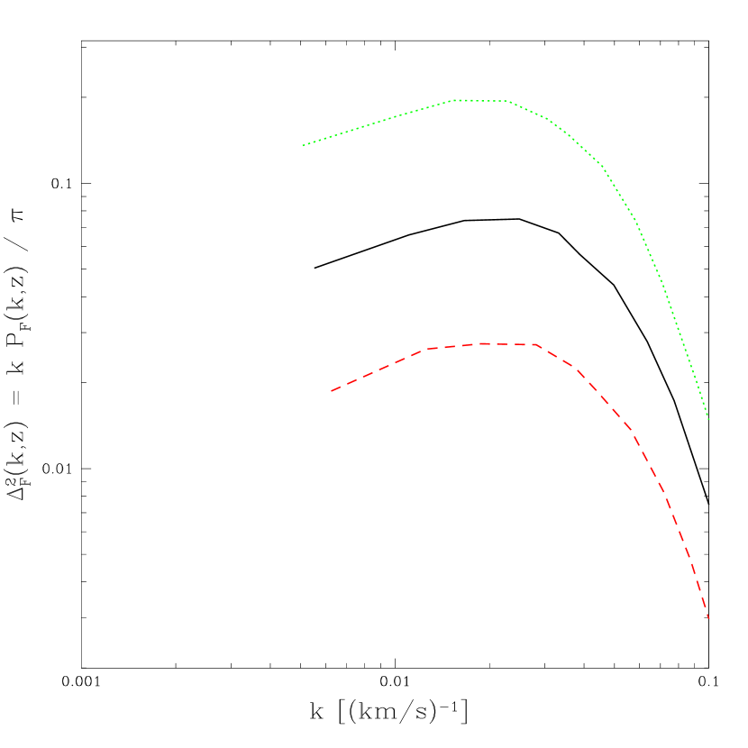
Figure 1: $P_{F}(k,z)$ prediction from our basic hydrodynamic simulation (FULL). The lines show, from bottom to top, $a=0.32$, 0.24, and 0.20, with $\bar{F}=0.85$, 0.67, and 0.4.

We see the expected increase in power with increasing redshift, due to the increase in mean absorption. This simulation box is too small to compare directly to the data, and we need simulations of many more models, but this is the base on which the analysis rests.

We show a resolution convergence test in Figure 2.

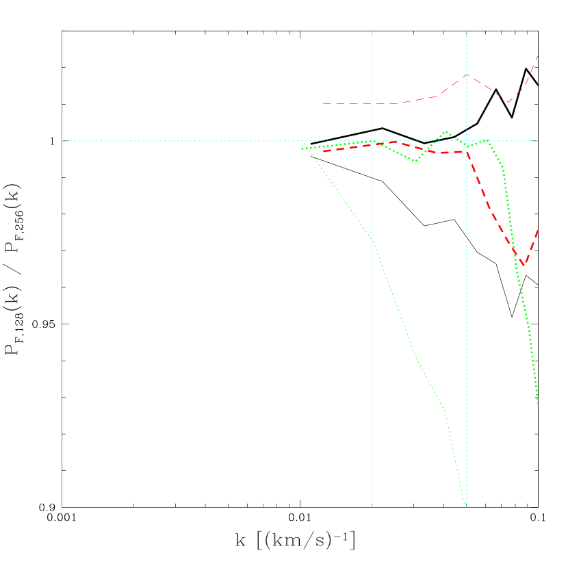
Figure 2: Resolution test for the hydrodynamic simulation, showing the ratio of $P_{F}(k,z)$ in a (5,128) run to $P_{F}(k,z)$ in a (5,256) run. The (red/dashed, black/solid, green/dotted) lines show $a=$(0.32, 0.24, 0.20), with $\bar{F}=$(0.85, 0.67, 0.4). Thin and thick lines, respectively, show before and after the redshift of reionization adjustment. The vertical cyan (dotted) lines mark the upper limits on $k$ used for SDSS and HIRES $P_{F}(k,z)$ measurements, while the horizontal dotted line guides the eye to 1. We use these same cyan/dotted lines in many figures (and occasionally another at $k=0.0013\,{\rm s\,km}^{-1}$, which marks the lower limit on $k$ used in our fits).

For this test we compared fully hydrodynamic runs of (5,256) and (5,128) (the latter has the same resolution as our base simulations).

Interpreting a resolution test of our hydrodynamic simulations requires some subtlety. Because of the detailed small-scale physics in the simulations, the time of reionization and the amount of heating during it are somewhat sensitive to resolution, even when we use the same ionizing background in both simulations (as we did for this resolution test – usually the homogeneous radiation background is computed from stars and AGN generated within the running simulation). For example: while the simulations do not include realistic radiative transfer, we do use a rough self-shielding approximation to attenuate the radiation background seen by high neutral density cells. In this resolution test the lower resolution simulation is $\sim 5000$ K hotter between reionization at $z\sim 10$ and $z\sim 7$, with the difference decreasing at lower redshift. Simple differences in the thermal history do not concern us in practice. In our power spectrum analysis we marginalize over the temperature-density relation and the small-scale smoothing level (which is sensitive to the full thermal history back to reionization), so changes of this kind will be automatically accounted for. In Figure 2 we first show (thin lines) the comparison when we correct only for the difference in temperature-density relation at the time of observation, i.e., differences in $T_{1.4}$ and $\gamma-1$. We see that, while the two resolutions agree to a few percent at $a=0.32$ and $a=0.24$, the disagreement at $a=0.2$ (and, probably more importantly, $\bar{F}=0.4$) is relatively large. We next allow for an adjustment in the filtering scale, equivalent to a change in the redshift of reionization. We implement this, as described in more detail below, by interpolating between HPM runs with reionization at $z=7$ heating the gas to 25000 K and reionization at $z=17$ with heating to 50000 K (in other contexts we have spot-checked that this interpolation is accurate). We require 27% of the difference between these two cases to produce the thick lines in Figure 2 (we also adjusted $\bar{F}$ in the two lower $z$ bins by 0.002 – a tiny amount relative to the uncertainties in $\bar{F}$). The agreement is excellent, indicating that any effect of limited resolution is degenerate with the nuisance parameters we are already marginalizing over. Some further investigation using HPM simulations with thermal histories matching those in the different resolution hydrodynamic simulations suggests that only about 1/3 of the effect is simply differences in thermal history. The other 2/3 must be an early-time smoothing of the gas by limited resolution.

The reader may at this point wonder why we believe that 5 $\,h^{-1}\,{\rm Mpc}$ simulations are sufficient for this resolution test. They would not be adequate if we needed to make any kind of correction using them directly, because the extrapolation to large scales would be very uncertain; however, we use them only to motivate a physical interpretation of the effect of limited resolution as a modification of the early-time thermal history (i.e., the reionization history). Since this seems to work so well, we believe the freedom we allow in the fits (see below) is sufficient to absorb any resolution-related error. This will be checked in the future with larger simulations.

We have two additional alternative-physics hydrodynamic runs. The first one does not have metal cooling and we call it NOMETAL, the second one does not have energy feedback from supernovae and we call it NOSN (the metals in the NOSN simulation still come from supernovae, i.e., they are not evenly distributed). Figures 3(a) and (b) show the ratio of $P_{F}(k,z)$ from NOSN and NOMETAL, respectively, to $P_{F}(k,z)$ from FULL.

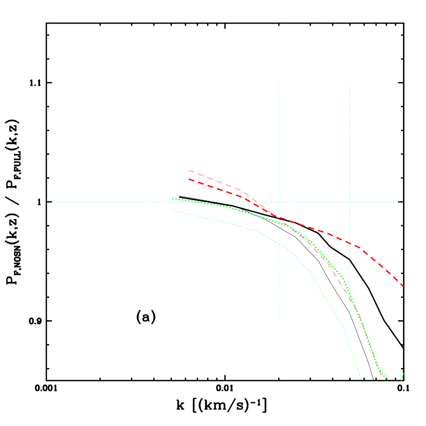
Figure 3: Comparison of hydro simulations including different physics. (a) shows the ratio of $P_{F}(k,z)$ in the NOSN (no energy feedback from supernovae) simulation to the FULL simulation. (b) shows $P_{\rm NOMETAL}/P_{\rm FULL}$ (NOMETAL means no metal cooling). The thick lines show the power after we correct for differences in the bulk temperature-density relations in the simulations, while the thin lines show the uncorrected power. The (red/dashed, black/solid, green/dotted) lines show $a=$(0.32, 0.24, 0.20), with $\bar{F}=$(0.85, 0.67, 0.4). The horizontal dotted line guides the eye to 1, while the vertical dotted lines mark the $k$ to which we use SDSS and HIRES data [$k<0.02~{}\,{\rm s\,km}^{-1}$ and $k<0.05~{}\,{\rm s\,km}^{-1}$, respectively].

The results from these simulations are not the same, at a level that, we will see later, does matter to us at the $\sim 1\sigma$ level. Some of the difference is simply a difference in the temperature-density relation within these simulations, which will be automatically accounted for when we use them to calibrate our HPM simulations. For example, the NOMETAL simulation is typically hotter, with smaller $\gamma-1$ — the $\sim 10$% disagreements seen in figure 3 are reduced to below $5$% when this is accounted for, as one can see by comparing Figure 5(a) and (c). These differences are thus not necessarily worrisome and only a full fit to the data can reveal their impact on the cosmological conclusions. When we perform our final fit to determine the mass power spectrum, we will include the differences between these simulations as an uncertainty in the fit by defining $P_{\rm hydro}=a~{}P_{\rm NOMETAL}+b~{}P_{\rm NOSN}+c~{}P_{\rm FULL}$, with $a$, $b$ and $c$ free parameters subject to the constraints $0<a,b,c<1$ and $a+b+c=1$. This procedure thus includes the systematic uncertainties that arise from these simulations, but also allows the possibility that simulations which better fit the data receive more weight.

2.3 Calibrating the HPM Simulations

Our hydro-particle-mesh (HPM) simulations model the IGM as simply particles evolving under gravity plus a pseudo-pressure term computed from an arbitrarily imposed temperature-density relation (Gnedin & Hui, 1998). They are not expected to simulate high density regions accurately because they do not contain shocked or cooled gas, but these regions occupy very little of the volume of the IGM and typically produce saturated absorption, and for both of these reasons have minimal influence on the Ly$\alpha$ forest power spectrum. The other approximation in the code we use (kindly provided by N. Gnedin) is the treatment of gas and dark matter with a single set of particles. Ultimately, the accuracy of the simulations must be verified by direct comparison with fully hydrodynamic simulations. As we will see, the agreement on $P_{F}(k,z)$ is very good. In fact, the HPM simulations agree with the hydrodynamic simulations as well as hydrodynamic simulations with different forms of galaxy feedback agree with each other.

We use the approximate HPM simulations for our main grid of models for two reasons: The obvious and most important one is that they are less costly to run – while we do not have a direct comparison with the fully hydrodynamic code that we use for the simulations in this paper, simulations using the publicly available ENZO code (O’Shea et al., 2004) require a factor of $\sim 50$ more CPU time than similar HPM simulations. Another useful advantage of the HPM simulations is that we can control the thermal history in them very easily. It is unlikely that we will ever be able to predict the thermal history from first principles using a hydrodynamic simulation, because of uncertainty in the simulation of radiation sources. Therefore, any proper analysis of the Ly$\alpha$ forest observations must marginalize over all plausible thermal histories. While it will certainly be possible in the future to manipulate fully hydrodynamic simulations to achieve this marginalization (this has been done on a small scale before, e.g., Schaye et al. (2000)), for now we do it using HPM simulations. We do not, however, assume that the HPM simulations are perfectly accurate. In this subsection we explain how we use a limited set of hydrodynamic simulations to calibrate the HPM simulations, i.e., to correct for any error in the HPM simulations.

We compare the hydrodynamic simulations discussed in §2.2 to a (10,256) HPM simulation with identical initial conditions. We use $N=256^{3}$ to match the resolution of our (20,512) simulations. We show the convergence with the time step in Figure 4.

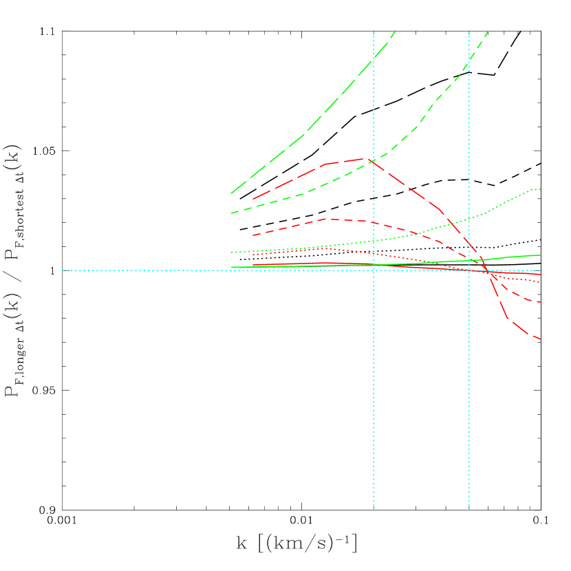
Figure 4: Convergence of $P_{F}(k,z)$ with decreasing time step size for the (10,256) HPM simulations that we compare to hydro simulations. Note that, of the simulations of this size, only the ones with the smallest timestep (most total steps) are used in our analysis. The denominator is the result for 876 times steps down to $z=1.5$, while solid, dotted, dashed, and long-dashed lines show, respectively, 429, 205, 89, and 42 steps. Red, black, and green indicate $P_{F}(k,z)$ at, respectively, $a=0.32$, 0.24, and 0.20, with $\bar{F}=0.85$, 0.67, and 0.4 (these run from bottom to top in each case when looking at $k=0.05\,{\rm s\,km}^{-1}$).

We use 876 steps down to $z=1.5$, although we have checked explicitly that 205 would have been sufficient to produce the same final $P_{L}$ result (note that we use the fully converged HPM simulation for our comparison with full-hydro simulations, not the corrected long-timestep HPM simulations discussed below).

Figures 5(a,b,c) show the HPM simulation compared to the three hydrodynamic simulation versions (FULL, NOSN, NOMETAL).

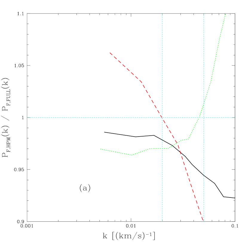
Figure 5: Comparison of the hydrodynamic results to the HPM results, for the same initial conditions and temperature-density relation. (a), (b), and (c) show, respectively, the comparison for the FULL, NOSN, and NOMETAL hydro simulations. The (red/dashed, black/solid, green/dotted) lines show $a=$(0.32, 0.24, 0.20), with $\bar{F}=$(0.85, 0.67, 0.4).

In each case we have used the temperature-density relation computed from the hydro simulation when creating the HPM spectra. Operationally, we estimate $T_{1.4}$ and $\gamma-1$ for the hydro simulation by a least absolute deviation fit (Press et al., 1992) to $\ln T$ vs. $\ln(\rho/\bar{\rho})$, limited to the range $1<\rho/\bar{\rho}<2$ (there is no unambiguously best way to make this estimate). We see that the agreement is generally quite good in the $k$ range that we use, although this is less true at $z=4$, $\bar{F}=0.4$. The general increase in disagreement at $k\sim 0.03\,{\rm s\,km}^{-1}$ can be understood qualitatively by looking forward to Figure 13, which shows the parameter dependence of $P_{F}(k,z)$. We see that this scale corresponds to the scale where thermal broadening suppression of the power is rapidly becoming significant. Furthermore, changes in pressure history (i.e., reionization) are becoming more important, and the “fingers of god”-like suppression of small-scale power by non-linear peculiar velocities becomes so significant that increasing the linear power actually begins to reduce the flux power. In other words: all of the details that make HPM an approximation are becoming significant for $k\gtrsim 0.03\,{\rm s\,km}^{-1}$. It is not entirely clear why the disagreement generally becomes substantially worse at $z=4$, but it seems likely that the hydrodynamic simulation has better effective resolution here, where resolution is most important (e.g., see Figure 9).

When running our standard HPM simulations, we usually use the same thermal history to compute the pressure term. We turn the pressure on at $z=7$, and then use linear interpolation in $\ln T_{1.4}$, $\gamma-1$, and $\ln(1+z)$ to connect the points $(T_{1.4},~{}\gamma-1,~{}z)=$(24511 K, 0.0, 7.0), (19939 K, 0.2, 3.9), (19542 K, 0.3, 3.0), and (20071 K, 0.55, 2.4), with the temperature decreasing like $a^{-1}$ and constant $\gamma-1$ at lower $z$. This does not exactly match the hydro simulations, e.g., FULL has $(T_{1.4},~{}\gamma-1,~{}z)=$(15527 K, 0.0, 7.33), (21180 K, 0.23, 5.25), (18754 K, 0.47, 4.00), (16618 K, 0.55, 3.17), (14910 K, 0.58, 2.57), (13561 K, 0.6, 2.12). To gauge the effect of the difference, we ran an HPM simulation using these points for the interpolation. Figure 6 shows that the results barely change, i.e., changes in the thermal history at relatively low redshift do not have much effect on $P_{F}(k,z)$.

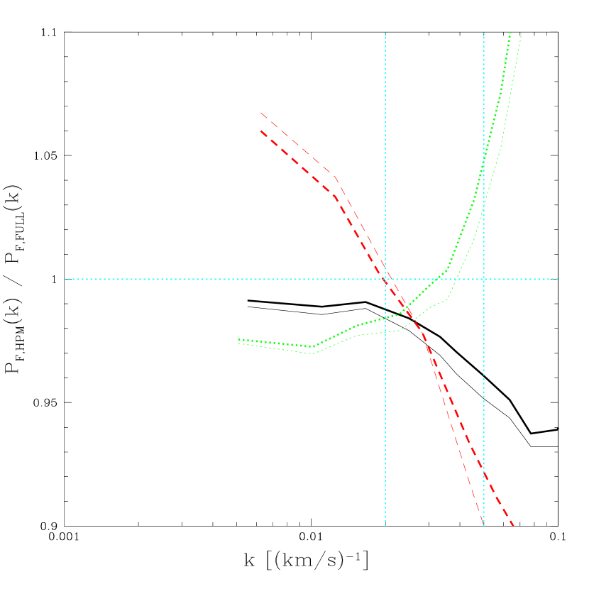
Figure 6: Unimportance of the late-time thermal history assumed in the HPM simulations. The thick lines show the $P_{\rm HPM}/P_{\rm hydro}$ ratio when the pressure in the HPM simulation is computed using the true thermal history in the hydrodynamic simulation, while the thin lines show the same for our default (closer to observed) thermal history (see text for numbers). The (red/dashed, black/solid, green/dotted) lines show $a=$(0.32, 0.24, 0.20), with $\bar{F}=$(0.85, 0.67, 0.4).

This is not to say that the thermal history is irrelevant – we will show below that early reionization can substantially smooth the gas, and we will allow for this in our fits.

We use these results as a correction to our larger HPM simulation results by multiplying the $P_{F}(k,z)$ prediction from the larger simulations by the ratio $P_{\rm hydro}/P_{\rm HPM}$. We account for the dependence of this correction on power spectrum amplitude and $\bar{F}$, but not temperature-density relation or power spectrum shape, since this would require more hydro simulations. Since the corrections are small, and the allowed variations in these parameters are also small, the change in the correction should be negligible. The procedure used to extrapolate the simulations to large scales not covered by the simulation is described below in section 2.8.

Incidentally, we have also compared the results of a pure PM run to the hydrodynamic simulation (using the same code as for HPM, just without the pressure term). Figure 7 shows this along with the HPM comparison.

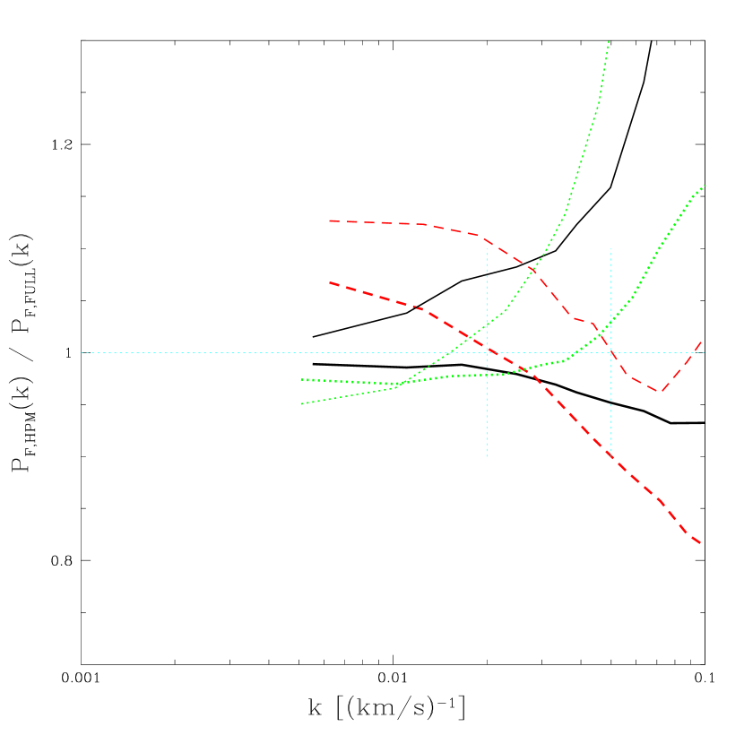
Figure 7: Comparison of PM (thin lines) vs. HPM (thick lines) relative to hydrodynamic results, for the same initial conditions and temperature-density relation. The (red/dashed, black/solid, green/dotted) lines show $a=$(0.32, 0.24, 0.20), with $\bar{F}=$(0.85, 0.67, 0.4).

In contrast to the findings of Meiksin & White (2001), we find that the pressure component in the HPM simulation substantially improves the agreement with the hydrodynamic simulation, in the way that one would intuitively expect, i.e., the PM result has too much small scale power (it is less obvious what is happening at the lowest redshift). While corrections need to be made in either case, our tests suggest HPM is as good or better than PM. However, given the recent computational advances in the development of fast fixed grid hydrodynamic codes (Trac & Pen, 2004), there may be no need to use these approximate methods in the future.

2.4 $20\,h^{-1}\,{\rm Mpc}$ and $40\,h^{-1}\,{\rm Mpc}$ HPM Simulations

Figure 8 shows a test for systematic error in $P_{F}(k,z)$ related to finite box size, comparing $P_{20,256}$ to $P_{40,512}$.

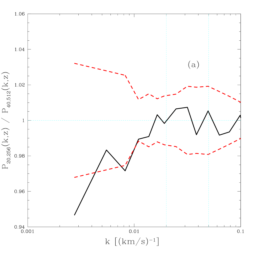
Figure 8: Box size test (note small range on the vertical axis). Black, solid line: ratio of $P_{20,256}$ to $P_{40,512}$, averaged over 8 and 6 simulations, respectively, with different seeds. Red, dashed line: plus and minus the rms error on the mean for each bin (estimated from the variance between the eight $N=256^{3}$ runs). (a, b, c) show $a=$(0.32, 0.24, 0.20), with $\bar{F}=$(0.85, 0.67, 0.4).

Note that, unlike most of our tests, we cannot perform a box size test with identical initial conditions in each simulation. To suppress the resulting larger statistical fluctuations, we averaged $P_{20,256}$ over eight runs with different seeds, and $P_{40,512}$ over six runs. We see that any systematic error in the $20\,h^{-1}\,{\rm Mpc}$ boxes is for the most part limited to be $\lesssim 2$%, although there probably is some error at that level. This error alone might not compel us to go to $L=40\,h^{-1}\,{\rm Mpc}$ simulations, but we need to predict the power spectrum on somewhat larger than $20\,h^{-1}\,{\rm Mpc}$ scales anyway, and the larger boxes give much smaller statistical errors per box, at fixed $k$.

Figure 9 shows the ratio $P_{20,256}/P_{20,512}$, demonstrating clearly that (40,512) simulations do not have sufficient resolution.

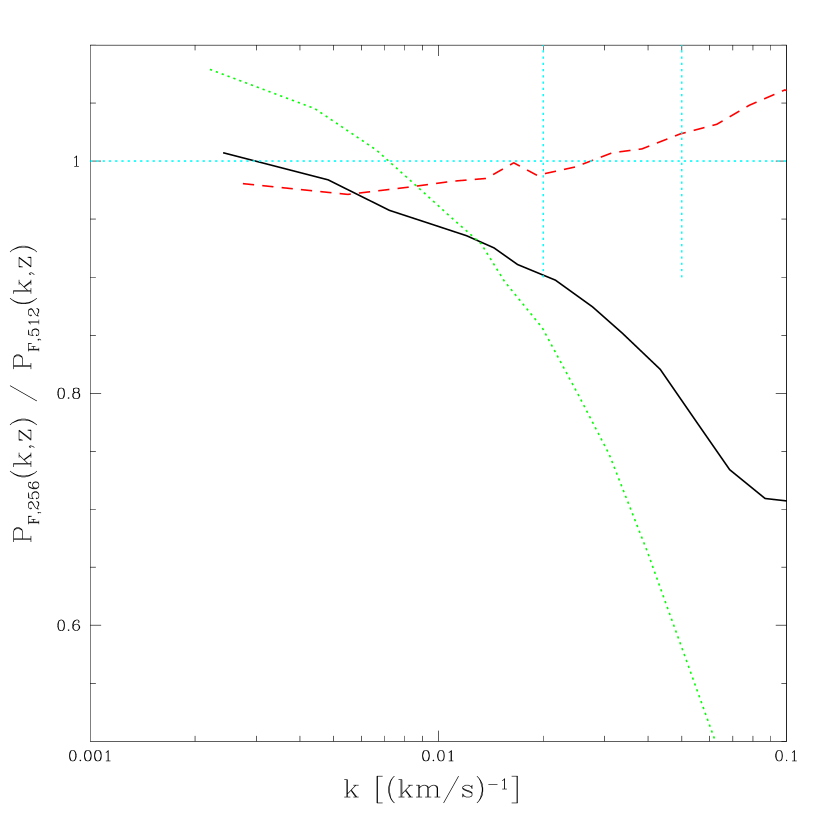
Figure 9: Resolution correction factor for the (40,512) HPM simulations. Plotted is the ratio of $P_{20,256}$ to $P_{20,512}$. Red/dashed, black/solid, and green/dotted indicate $P_{F}(k,z)$ at, respectively, $a=0.32$, 0.24, and 0.20, with $\bar{F}=0.85$, 0.67, and 0.4.

Note that, while the eye is drawn to the very large difference at high $k$ and $z$, for the scales probed by SDSS data [$k<0.02~{}\,{\rm s\,km}^{-1}$] the errors are no more than 15%, and usually less. The counter-intuitive small increase in small-scale power with decreasing resolution at $a=0.32$ is probably a case of limited resolution reducing the small-scale smoothing by peculiar velocities more than it reduces the real-space power. This prompts us to use $L=40\,h^{-1}\,{\rm Mpc}$ simulations, but correct them for the resolution error. We do this by dividing by the correction factor given by Figure 9. Including the hydro correction, the formula for our predicted $P_{F}(k,z)$ is then:

$$P_{F}(k,z)=P_{40,512}~{}\frac{P_{20,512}}{P_{20,256}}~{}\frac{P_{\rm hydro}}{P_{\rm HPM}}.$$ (1)

As we discuss below, we also tried fitting to observations using predictions based simply on (20,512) simulations, i.e., $P_{F}(k,z)=P_{20,512}~{}P_{\rm hydro}/P_{\rm HPM}$, and get essentially the same result, suggesting that several potential problems (limited box size, statistical errors, accuracy of the resolution correction) are not significant. Note that the convergence of the hydrodynamic simulations is a separate issue.

Finally, we need to check the timestep convergence of these HPM simulations. Because we wanted literally hundreds of simulations to cover the pre-SDSS allowed range of parameter space, and to make sure we did not have statistical errors, we intentionally ran the main grid with rather large time steps ($\sim 20-30$ steps to reach $z=1.5$). We will have to make a small correction for the error this causes. Figures 10 (a-c) show the tests for each relevant simulation size.

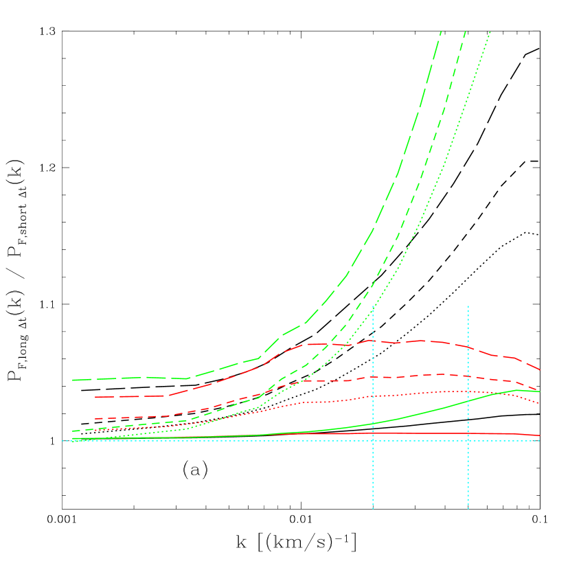
Figure 10: Time-step convergence test. (a-c) show $P_{F}(k,z)$ from (40,512), (20,512), and (20,256) simulations, respectively, for different numbers of time steps relative to $P_{F}(k,z)$ for the largest number we tried. The timesteps down to $z=1.5$ used for the (denominators, solid lines, dotted, dashed, long-dashed) are (479, 227, 94, 41, 20), (589, 256, 116, 50, 20), and (702, 336, 158, 67, 33) for (a-c). In each case $a=$(0.32, 0.24, 0.20), with $\bar{F}=$(0.85, 0.67, 0.4) run from bottom to top at $k=0.05\,{\rm s\,km}^{-1}$.

We make the corrections in the usual way, i.e., multiplying the main grid $P_{F}(k,z)$ by $P_{{\rm short}\Delta t}/P_{{\rm standard}\Delta t}$ (separately for each box size and resolution). The time savings comes about because we do not allow the correction to depend on power spectrum shape, or compute it for more than one random seed for the initial conditions (we do include dependence on power spectrum amplitude, $\bar{F}$, $T_{1.4}$, and $\gamma-1$, because these do not require extra simulations). We see that a huge savings in time can be obtained at a small price in accuracy.

2.5 Summary of Numerical Simulation Error Control

We emphasize that our analysis attempts to fully account for all of the possible numerical error sources discussed above. Any residual systematic error can only enter through imperfections in the corrections we make. The finite resolution of the hydrodynamic simulations is allowed for by introducing extra freedom in the filtering scale of the gas (Gnedin et al., 2003), which we showed in Figure 2 has an effect practically equivalent to a change in resolution. The sensitivity to physics details in the hydrodynamic simulations, shown in Figure 3, is allowed for by making the hydrodynamic simulation prediction an average over the three physics versions, with the relative weightings of the average as free parameters. The error in the HPM approximation is corrected by comparison to the hydrodynamic simulations, with the uncertainty in extrapolation from $10\,h^{-1}\,{\rm Mpc}$ box size to larger scales accounted for by a free parameter that allows anything between a constant value of $P_{F}(k,z)$ and a constant slope of $P_{F}(k,z)$. Limited box size in our $40\,h^{-1}\,{\rm Mpc}$ simulations is not a significant source of statistical or systematic error, as shown by Figure 8 and the fact that our results using only $20\,h^{-1}\,{\rm Mpc}$ simulations are consistent (see below, Table 2). Limited resolution in the (40,512) simulations is corrected for using full grids of (20,512) and (20,256) simulations, with any remaining resolution error in the (20,512) simulations incorporated into the hydrodynamic correction. Finally, error from insufficiently small timesteps in the main grids of HPM simulations is corrected by comparison to fully converged simulations.

2.6 High Density Absorbers and UV Background Fluctuations

Very high density systems are not necessarily well reproduced by our hydrodynamic simulations (Cen et al., 2003; Miralda-Escude et al., 1996; Gardner et al., 2001; Nagamine et al., 2004; Viel et al., 2004a). McDonald et al. (2005) investigate this issue in some detail, finding that the presence of damping wings is important, although much of the effect comes from systems below the traditional cutoff for damped Ly$\alpha$ systems (neutral column density $N(\mbox{H\,{\scriptsize I}\ })=2\times 10^{20}{\rm~{}atoms~{}cm^{-2}}$, Wolfe et al. (1986); Smith et al. (1986)). McDonald et al. (2005) give templates for the contribution of high density systems to $P_{F}(k,z)$, constrained by the observed column density distribution of these systems (Péroux et al., 2003a, b; Prochaska & Herbert-Fort, 2004). We reproduce examples from the two templates that we use in this paper in Figure 11.

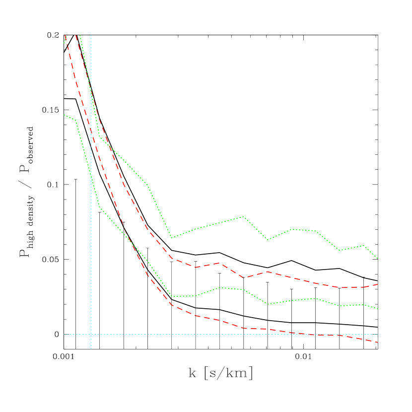
Figure 11: Change in $P_{F}(k,z)$ when DLAs and LLSs (systems with $N(\mbox{H\,{\scriptsize I}\ })>1.6\times 10^{17}{\rm~{}atoms~{}cm^{-2}}$) with the observed column density distribution are inserted into mock spectra of the Ly$\alpha$ forest, relative to the observed Ly$\alpha$ forest $P_{F}(k,z)$, from McDonald et al. (2005). The upper curves show the case where the high density systems are inserted randomly, while for the lower curves the LLSs and DLAs were inserted at the highest density maxima in mock Ly$\alpha$ forest spectra. Red (dashed), black (solid), and green (dotted) lines show $z=2.2$, 3.2, and 4.2. The error bars indicate the fractional error on the observed $P_{F}(k,z)$ at $z=3.2$ (the errors at $z=2.2$ are very similar, while the errors at $z=4.2$ are $\sim 2$ times bigger). Note that a consistent systematic error that is $1\sigma$ for any single point is very significant, because we have many $z$ and $k$ bins to average over.

The differences between the two cases in the figure is that in one case the high density systems are located at peaks in the mock density field, while in the other they are located randomly. Relative to the case when the systems are located randomly, when the systems are located in high density regions there is little effect on the small-scale power, because the affected regions are already saturated (the relatively low equivalent width systems, which account for the small scale power, produce little change when they are inserted). The randomly located case is not realistic, but we include it to show that our fits are not sensitive to this kind of detail (see below). Based on the discussion in McDonald et al. (2005), we will assign an overall 30% error to the size of this effect in our fits. A more careful study could probably reduce this error, but our results are not especially sensitive to it.

McDonald et al. (2005); Croft (2004), and Meiksin & White (2004) investigate the potential influence of a fluctuating UV background on $P_{F}(k,z)$. These papers find an effect that increases dramatically as the mean free path for an ionizing photon decreases with increasing redshift. The effect only becomes significant at the high end of the redshift range we consider in this paper. Figure 12 shows examples of the templates we use to include this effect in our fitting, taken from McDonald et al. (2005).

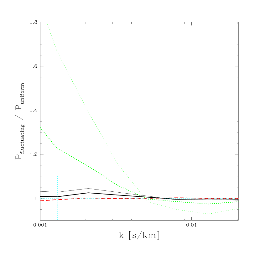
Figure 12: Effect of a fluctuating UV background, from McDonald et al. (2005). Thick lines show the template we use in our standard fitting, when we assume all of the UV background comes from quasars. Thin lines show a case where the mean free path for ionizing photons in the IGM has been arbitrarily reduced by a factor of two and is meant to show the worst case scenario (the fluctuations increase with decreasing mean free path). Red (dashed), black (solid), and green (dotted) lines show $z=2.05$, 3.29, and 4.58. The thick and thin dashed lines are indistinguishable.

These correspond to the quasar luminosity function from Fan et al. (2002), with quasar lifetime of $10^{7}$ years, and include light-cone effects described by Croft (2004). The models in Figure 12 are the extreme (maximum fluctuation) cases. More detailed analysis of other models is presented in McDonald et al. (2005). In contrast to the case of damping wings, we have little direct constraint on the redshift evolution of this effect. We will include nuisance parameters for both the amplitude and evolution of the effect in our fits, and find that including this freedom increases the error on the linear power spectrum measurement, but does not change the central value significantly.

2.7 Parameter Dependence of $P_{F}$

We now discuss the parameter dependence of $P_{F}(k,z)$ in our simulations. Much of this has been shown already in the McDonald (2003) plots of the three-dimensional flux power spectrum, but it is useful to see directly the effects on the one-dimensional $P_{F}(k,z)$. Figures 13(a-c) show examples of the fractional change in $P_{F}(k,z)$ when $\Delta_{L}^{2}(k_{p},z_{p})$ is increased by 10%, $n_{\rm eff}(k_{p},z_{p})$ is increased by 0.05, $\alpha_{\rm eff}(k_{p},z_{p})$ is increased by 0.05, $\bar{F}$ is increased by 0.01, $T_{1.4}$ is increased by 3000 K, $\gamma-1$ is decreased by 0.1, or reionization is moved from $z=7$ to $z=17$.

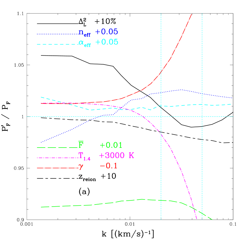
Figure 13: Parameter dependence of $P_{F}(k,z)$ in $(40,512)$ simulations, as a ratio of $P_{F}(k,z)$ after one parameter, $p$, is changed by $\Delta p$ to $P_{F}(k,z)$ for a central set of parameters. Solid (black) line: $\Delta_{L}^{2}(k_{p},z_{p})$ increased by 10%, dotted (blue) line: $\Delta n_{\rm eff}(k_{p},z_{p})=0.05$, dashed (cyan) line: $\Delta\alpha_{\rm eff}(k_{p},z_{p})=0.05$, long-dashed (green) line: $\Delta\bar{F}=0.01$, dot-dashed (magenta) line: $\Delta T_{1.4}=3000$ K, dot-long-dashed (red) line: $\Delta\gamma=-0.1$, dashed-long-dashed (black) line: $\Delta z_{\rm rei}=10$. The panels show central values representing the middle and extremes of our redshift range: (a) $\bar{F}=0.85$, $a=0.32$, (b) $\bar{F}=0.67$, $a=0.24$, (c) $\bar{F}=0.4$, $a=0.2$. Note that these figures are intended primarily as a qualitative demonstration, as detailed corrections have not been applied (e.g., the up-turn of the $\Delta_{L}^{2}(k_{p},z_{p})$ dependence at very high $k$ is an effect of limited resolution).

The starting values are our simulation standard $\Delta^{2}(k_{s}=1~{}{\rm h/Mpc},a_{s}=0.24)=0.26$, $n_{\rm eff}(k_{s},a_{s})=-2.3$, $\alpha_{\rm eff}(k_{s},a_{s})=-0.2$, $T_{1.4}=17000$ K, and $\gamma-1=0.6$, with $\bar{F}=$(0.85, 0.67, 0.4) at $a=$(0.32, 0.24, 0.20). We used (40,512) simulations for this figure. $P_{F}(k,z)$ for the central model (the denominator in the plot) is taken essentially directly from a simulation output, but the changes involve some interpolation to achieve the desired size of change.

The parameter dependences are generally non-trivial. Increasing $\Delta_{L}^{2}(k_{p},z_{p})$ enhances the power on large scales, but actually suppresses the power on small scales. McDonald (2003) shows that this is a finger-of-god-like effect of peculiar velocities suppressing power along the line of sight: if the amplitude is higher the velocities are higher, which leads to a suppression of power on small scales. Note that these dependences can be affected slightly by limited resolution at high $k$, e.g., when $\Delta_{L}^{2}(k_{p},z_{p})$ is increased in (20,512) simulations the suppression of $P_{F}(k,z)$ continues to increase at $k>0.04\,{\rm s\,km}^{-1}$. Changing $n_{\rm eff}(k_{p},z_{p})$ produces a fairly simple and expected change in the slope of $P_{F}(k,z)$, except at high $k$ and low $z$. Changing $\alpha_{\rm eff}(k_{p},z_{p})$ produces curvature in $P_{F}(k,z)$, although the effect almost disappears at low $z$. $\bar{F}$ produces a relatively flat, large change, which is commonly assumed to be degenerate with $\Delta_{L}^{2}(k_{p},z_{p})$, although we see that the shapes are not the same, nor are the relative effects at different redshifts: as a result, the data can break the degeneracy within the flux power spectrum analysis itself without the need to bring in external constraints. Increasing $T_{1.4}$ primarily suppresses the power at high $k$, not surprisingly, although it also produces a small change in large-scale bias. Decreasing $\gamma-1$ produces an overall bias, but also a sharp increase in power at high $k$, in the two lower redshift cases. This is an indication that the power is sensitive to structures with overdensity greater than 1.4, since their temperature is reduced by a decrease in $\gamma-1$, leading to reduced thermal broadening suppression of power. At $z=4$ (and, more importantly, $\bar{F}=0.4$), $\Delta=1.4$ appears to be the most relevant overdensity. Finally, increasing the redshift of reionization allows more time for pressure to suppress small-scale structure (Jeans smoothing). The power suppression extends to smaller $k$ than the thermal broadening effect, because it acts on the three-dimensional field instead of only along the line of sight. This effect decreases rapidly with decreasing redshift and increasing $\bar{F}$, allowing us to constrain it in a full fit to the data.

2.8 Combining and Interpolating Between Simulations

In this subsection we describe the procedure we use to turn hundreds of simulations (and more than 100,000 power spectrum calculations, after variations of $a$, $\bar{F}$, $T_{1.4}$, and $\gamma-1$) into a prediction for $P_{F}(k,z)$ for any given set of input parameters. There are some subtleties in this process that we describe in full, in preparation for releasing a code that can be used as a black box calculator of the Ly$\alpha$ forest $\chi^{2}$. Our simulation set can not be described as a simple grid in parameter space, so in Figure 14 we plot all of the points we cover in the $\Delta_{L}^{2}(k_{p},z_{p})$-$n_{\rm eff}(k_{p},z_{p})$ plane, for (40,512).

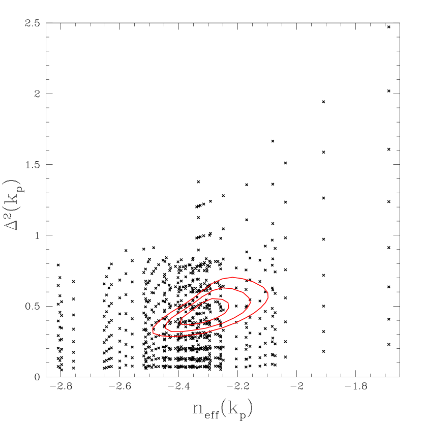
Figure 14: Each point shows the position of one of our (40,512) simulation outputs in the linear power spectrum amplitude-slope plane, at $k_{p}=0.009~{}\,{\rm s\,km}^{-1}$. To distinguish between multiple runs using the same input power spectrum, the points are plotted at the effective position computed from the power as realized in the randomly generated initial conditions. For comparison, the red lines show the 1, 2, and 3 $\sigma$ error contours (at $z_{p}=3$) that we find later in the paper by fitting the observational data.

Our grids of (20,512) and (20,256) simulations are almost identical to this (40,512) grid.

The adopted interpolation method is designed to deal with some of the special features of our problem. The calculation of the Ly$\alpha$ forest $\chi^{2}$ is an essential ingredient that goes into joint parameter estimation, together with similar $\chi^{2}$ calculations from the CMB, galaxy clustering, supernovae and other ingredients. The CMB and galaxy clustering depend on linear theory calculations, so for each model we need to run a linear perturbation calculation like CMBFAST (Seljak & Zaldarriaga, 1996), which is relatively fast. To determine the error distributions in a parameter space of models one typically uses the Monte Carlo Markov Chain (MCMC) method, which requires $\chi^{2}$ calculations for tens of thousands of models.

Each Ly$\alpha$ forest simulation is relatively expensive (compared to a CMBFAST run), while simultaneously only providing a noisy estimate of the quantity of interest. To minimize the number of simulations needed, we take advantage of the fact that $P_{F}(k,z)$ in our simulations has a smooth $k$ dependence, and a smooth dependence on the input parameters. We condense every $P_{F}(k)$ calculation into a few numbers using a fitting formula, and then condense this information even further using another fitting formula for the dependence of the parameters describing $P_{F}(k)$ on the more fundamental cosmological and Ly$\alpha$ forest model parameters. The idea is to use the minimum number of parameters needed to describe the true (infinite simulation limit) power, in contrast to a more standard local interpolation between $P_{F}(k)$ predictions binned by $k$.

The $P_{F}(k)$ fitting formula is simple, motivated by the smoothness of the power spectrum in the models we simulate.

$$\ln P_{F}(k)=\sum_{\alpha=0}^{N_{\rm log}}P_{\alpha}~{}\left[\ln\left(k/k_{\star}\right)\right]^{\alpha}+\sum_{\alpha=1}^{N_{\rm lin}}P_{\alpha+N_{\rm log}}~{}k^{\alpha}~{},$$ (2)

where $k_{\star}=0.3(\,h^{-1}\,{\rm Mpc})^{-1}$ and $N_{\rm log}$ and $N_{\rm lin}$ can be chosen to give the appropriate amount of freedom (we use 3 and 2 terms, respectively, as our standard). For each simulated $P_{F}(k)$ we determine the parameters $P_{\alpha}$ by a $\chi^{2}$ fit weighted by statistical errors on $P_{F}(k)$ bands determined by measuring the variance in a set of simulations of one model with many different seeds for the random initial condition generator.

The general structure of our method for associating $P_{\alpha}$ with physical model parameters $p_{i}$ (e.g., linear power spectrum amplitude, $\bar{F}$, etc.), is as follows: we define a conveniently transformed set of model parameters, $p_{i}$, and use them in a linear least-squares fit for the coefficients $A_{\alpha\nu_{1}\nu_{2}\nu_{3}...\nu_{N_{p}}}$ in the formula

$$P_{\alpha s}=\left(\prod_{i=1}^{N_{p}}\sum_{\nu_{i}=0}^{N_{i}}p_{is}^{\nu_{i}}\right)A_{\alpha\nu_{1}\nu_{2}\nu_{3}...\nu_{N_{p}}}~{},$$ (3)

where $s$ labels a simulation, $p_{is}$ means the value of the $i$th physical parameter in the $s$th simulation, there are $N_{p}$ parameters, and the term in parentheses should be thought of as an operator acting on $A_{\alpha\nu_{1}\nu_{2}\nu_{3}...\nu_{N_{p}}}$. Equation 3 is just a compact way of writing the formula one effectively uses for multi-polynomial interpolation, e.g., for $N_{p}=2$ parameters and $N_{i}=1$ we have $P_{\alpha s}=A_{\alpha 00}+A_{\alpha 01}~{}p_{1s}+A_{\alpha 10}~{}p_{2s}+A_{\alpha 11}~{}p_{1s}~{}p_{2s}$, i.e., the formula for bi-linear interpolation. Equation 3 has the important practical advantage of being linear in all the parameters, so it is easy to perform multiple fits to $\sim 10^{5}$ data points. After some experimentation, we chose $\ln[-\ln(\bar{F})]$, $\ln T_{1.4}$, and $\ln[2-0.7~{}(\gamma-1)]$ to be the parameters $p_{i}$ for the Ly$\alpha$ forest model. Reionization will be treated outside this formalism, as discussed below. All that remains is to define a way to turn a given linear power spectrum, say, from CMBFAST, into the rest of $p_{i}$.

In the infinite-dimensional space of possible input linear power spectra, we have many relatively smooth models, from pure power laws with $-2.75\leq n\leq-2.1$, to $\Lambda$CDM transfer function models with $-2.8\leq n_{\rm eff}(k_{p},z_{p})\leq-2.15$ and $-0.37\leq\alpha_{\rm eff}(k_{p},z_{p})\leq-0.03$, to the primordial black hole models described in Afshordi et al. (2003) (these have extra white noise power that dominates at small scales), to warm dark matter models where the small-scale power is erased (Narayanan et al., 2000). Nevertheless, it is easy to produce a model that cannot be obtained exactly by interpolation between the models we have (e.g., we do not include variations in the baryon density, because we do not expect their effect to be independently measurable from $P_{F}(k,z)$). We deal with this problem by defining a set of parameters to project any power spectrum onto, akin to $\Delta_{L}^{2}(k_{p},z_{p})$, $n_{\rm eff}(k_{p},z_{p})$, and $\alpha_{\rm eff}(k_{p},z_{p})$. The basic formula for these parameters is

$$\Delta^{2}_{l}=\int_{\ln k_{\rm min}}^{\ln k_{\rm max}}d\ln k~{}\Delta_{L}^{2}(k)~{}P_{l}[x(k)]\exp[-(kR_{c})^{2}]~{},$$ (4)

where $x(k)=\ln(k/k_{0})/\ln(k_{\rm max}/k_{0})$, $k_{0}=(k_{\rm max}k_{\rm min})^{1/2}$, $k_{\rm min}=0.126(\,h^{-1}\,{\rm Mpc})^{-1}$, $k_{\rm max}=15.8(\,h^{-1}\,{\rm Mpc})^{-1}$, $R_{c}=0.2\,h^{-1}\,{\rm Mpc}$, and $P_{l}(x)$ is a Legendre polynomial of order $l$ (e.g., 1, $x$, $(3x^{2}-1)/2$, …). This is nothing more than a convenient way of defining a measure of the amplitude, slope, curvature, etc. of the power spectrum. There is nothing fundamental, or even decisively optimal, about the choice of weighting $P_{L}(k)$ by $k^{3}$ in Equation 4 (we tried, and could almost just as well have used, other powers of $k$). $k_{\rm min}$ was chosen to include the smallest $k$ in our simulations. The weighting term controlled by $R_{c}$ was introduced to reduce the influence of high-$k$ power on our interpolation parameters ($\Delta^{2}_{l}$), after we found by running simulations with spikes of power in relatively narrow bands of $k$ that the very high $k$ linear power we are suppressing by this term has diminishing effect on the Ly$\alpha$ forest flux power, presumably because of some combination of pressure smoothing and non-linear transfer of power from large to small scales (Hamilton et al., 1991; Zaldarriaga et al., 2003). The value $R_{c}=0.2\,h^{-1}\,{\rm Mpc}$ was chosen to maximize the accuracy of the fit to the simulations for the number of Legendre polynomial terms we use (generally 4). $k_{\rm max}$ was chosen to center the Legendre polynomials near the wavenumber $k_{s}=1(\,h^{-1}\,{\rm Mpc})^{-1}$ that we used as the pivot point when setting the power spectra in our simulations. When applying Equation 4 to our numerical simulations, we sum over the discrete set of mode amplitudes actually present in the simulation. Finally, for the parameters $p_{i}$ in Equation 3 we actually use $\ln\Delta^{2}_{0}$ and $\Delta^{2}_{i>0}/\Delta^{2}_{0}$, so that only the first evolves with redshift and the rest are pure measures of power spectrum shape.

We apply the above formalism to each type of simulation separately. When we need to extrapolate small-box simulations down to smaller $k$ than they contain directly, we assume the extrapolation should fall somewhere between $P_{F}(k)={\rm constant}$ and $d\ln P_{F}/d\ln k={\rm constant}$, i.e., $P_{F}(k)$ in the Ly$\alpha$ forest never decreases with decreasing $k$, and the second derivative is generally negative. We introduce a free parameter controlling our position between these limits. This issue is only significant when extrapolating the $L=10\,h^{-1}\,{\rm Mpc}$ hydrodynamic simulations and their comparison HPM simulations to our largest scales.

3 Fitting the Observed $P_{F}(k,z)$

In this section we explain how we perform $\chi^{2}$ fits to the observational data to estimate the linear power spectrum. We begin with the description of all the parameters that go into the fit. We then describe the data itself and present our main results next. The remainder of this section is devoted to the various consistency checks we performed, both using internal constraints from the data and modifying the standard fitting procedure.

3.1 Parameters

We vary 34 parameters, 3 of which are fixed for our primary result, but varied for consistency checks. We give a bulleted summary before defining each in detail. In brackets we give the actual number of parameters for each type.

• $\Delta_{L}^{2}(k_{p},z_{p})$, $n_{\rm eff}(k_{p},z_{p})$, $\alpha_{\rm eff}(k_{p},z_{p})$ (3)
  Standard linear power spectrum amplitude, slope, and curvature on the scale of the Ly$\alpha$ forest, assuming a typical $\Lambda$CDM-like Universe. $\alpha_{\rm eff}(k_{p},z_{p})$ is fixed to -0.23 for the main result.

• $g^{\prime}$, $s^{\prime}$ (2)
  Modifiers of the evolution of the amplitude and slope with redshift, to test for deviations from the expectation for $\Lambda$CDM. Fixed for main result.

• $\bar{F}(z_{p})$, $\nu_{F}$ (2)
  Mean transmitted flux normalization and redshift evolution.

• $T_{i=1..3}$, $\tilde{\gamma}_{i=1..3}$ (6)
  Temperature-density relation parameters, including redshift evolution.

• $x_{rei}$ (1)
  Degree of Jeans smoothing, related to the redshift and temperature of reionization.

• $f_{\rm SiIII}$, $\nu_{\rm SiIII}$ (2)
  Normalization and redshift evolution of the SiIII-Ly$\alpha$ cross-correlation term.

• $\epsilon_{n,i=1..11}$ (11)
  Freedom in the noise amplitude in the data in each SDSS redshift bin.

• $\alpha_{R}$ (1)
  Freedom in the resolution for the SDSS data.

• $A_{\rm damp}$ (1)
  Normalization of the power contributed by high density systems.

• $a_{\rm NOSN}$, $a_{\rm NOMETAL}$ (2)
  Admixture of corrections from the NOSN and NOMETAL hydrodynamic simulations.

• $A_{\rm UV}$, $\nu_{\rm UV}$ (2)
  Normalization and redshift evolution of the correction for fluctuations in the ionizing background.

• $x_{\rm extrap}$ (1)
  Freedom in the extrapolation of our small simulation results to low $k$.

The linear theory power spectrum, comprising the primary result of the paper, is described by an amplitude, $\Delta_{L}^{2}(k_{p},z_{p})=k_{p}^{3}P_{L}(k_{p},z_{p})/2\pi^{2}$, with normalization convention such that $\sigma_{L}^{2}=\int_{-\infty}^{\infty}d\ln k~{}\Delta_{L}^{2}(k)$, where $\sigma_{L}^{2}$ is the variance of the linear theory density field; slope, $n_{\rm eff}(k_{p},z_{p})=d\ln P_{L}/d\ln k\left.\right|_{z_{p},k_{p}}$, and curvature, $\alpha_{\rm eff}(k_{p},z_{p})=dn_{\rm eff}/d\ln k\left.\right|_{z_{p},k_{p}}$. Together these describe an approximate power spectrum:

$$\Delta^{2}_{L}(k,z)\simeq\left[\frac{D(z)}{D(z_{p})}\right]^{2}\Delta_{L}^{2}(k_{p},z_{p})\left[\frac{k}{k_{\star}(z)}\right]^{3+n_{\rm eff}(k_{p},z_{p})+1/2~{}\alpha_{\rm eff}(k_{p},z_{p})\ln\left[k/k_{\star}(z)\right]}~{},$$ (5)

where $k$ is measured in $\,{\rm km\,s}^{-1}$, with $z_{p}=3.0$ and $k_{p}=0.009\,{\rm s\,km}^{-1}$. We preserve the linear theory prediction that only the amplitude of the power spectrum evolves in comoving coordinates by defining $k_{\star}(z)=k_{p}[H(z_{p})/(1+z_{p})]/[H(z)/(1+z)]\simeq k_{p}[(1+z_{p})/(1+z)]^{1/2}$. We compute $D(z)$ and $H(z)$ for a typical $\Omega_{m}=0.3$ $\Lambda$CDM model, although at the level of our error bars this is indistinguishable from an Einstein-de Sitter model (i.e., $D(z)/D(z_{p})\simeq a/a_{p}$). In practice we actually measure these power spectrum parameters as deviations from a CMBFAST power spectrum for a flat $\Lambda$CDM model with $\Omega_{m}=0.3$, $h=0.7$, and $\Omega_{b}=0.04$, which has $\alpha_{\rm eff}(k_{p},z_{p})=-0.23$ and $n_{\rm eff}(k_{p},z_{p})=-2.26$ (the latter is for primordial power spectrum slope $n=1.0$). Note that $\alpha_{\rm eff}(k_{p},z_{p})$ only weakly changes with cosmological parameters. i.e. $-0.25<\alpha_{\rm eff}(k_{p},z_{p})<-0.15$ over the range of interest.

When we measure a growth factor we parameterize it by $g^{\prime}$ in $D(z)/D(z_{p})=(a/a_{p})^{g^{\prime}}$, where $g^{\prime}$ should not be measurably different from 1 for a standard cosmology. Unexpected evolution of the slope is parameterized by $n_{\rm eff}[z,k_{\star}(z)]=n_{\rm eff}(k_{p},z_{p})+s^{\prime}(z-z_{p})$. These parameters are included to test for deviations from the expected Einstein-de Sitter Universe, but are fixed to their expected values for the standard fit.

We describe $\bar{F}(z)$ by a power law in effective optical depth, $\bar{F}(z)=\exp(\ln[\bar{F}(z_{p})][(1+z)/(1+z_{p})]^{\nu_{F}})$. Even if the truth is not quite consistent with this representation, we expect that the power spectrum parameters will be mostly sensitive to the overall normalization, so this parameterization should be sufficient, i.e., small wiggles or curvature might lead to a bad fit to the redshift evolution of $P_{F}(k,z)$, but are not likely to cause significant bias in the extraction of $P_{L}(k)$.

We allow considerable freedom in the temperature-density relation, because it is possible that its evolution is not monotonic (Schaye et al., 2000; Ricotti et al., 2000; McDonald et al., 2001; Zaldarriaga et al., 2001). $T_{1.4}(z)$ is parameterized by quadratic interpolation between three points, $T_{1}=T_{1.4}(z=2.4)$, $T_{2}=T_{1.4}(z=3.0)$, $T_{3}=T_{1.4}(z=3.9)$. Similarly, $(\gamma-1)(z)$ is described by three parameters at the same redshifts as $T_{1.4}$. Because we have only weak observational constraints, but theoretical limits $0\lesssim\gamma-1\lesssim 0.6$ (Hui & Gnedin, 1997), we use a parameterization that lends itself to enforcing an upper and lower limit. The exact form is $(\gamma-1)(z)=0.7(\tanh[\tilde{\gamma}(z)]+1)/2-0.05$, where $\tilde{\gamma}(z)$ is defined by quadratic interpolation between $\tilde{\gamma}_{1}=\tilde{\gamma}(z=2.4)$, $\tilde{\gamma}_{2}=\tilde{\gamma}(z=3.0)$, $\tilde{\gamma}_{3}=\tilde{\gamma}(z=3.9)$. This form naturally applies the constraint $-0.05\lesssim\gamma-1\lesssim 0.65$. We add $(\tilde{\gamma}_{i}/10)^{2}$ to $\chi^{2}$ to prevent the parameters from wandering off to infinity.

Differing reionization histories are included by multiplying our standard power spectrum prediction by $1+f(x_{rei})[P_{{\rm high}~{}z}(k,z)/P_{\rm standard}(k,z)-1]$, where $P_{{\rm high}~{}z}$ is an HPM simulation in which the temperature was set to 50000 K at $z=17$ and evolved as a power law down to our usual values at $z<4$, while $P_{\rm standard}$ was our standard case with $T=25000$ K at $z=7$. We use $f(x_{rei})=1.6~{}(\tanh[x_{rei}]+1)/2-0.3$, and add $(x_{rei}/10)^{2}$ to $\chi^{2}$. The lower limit $x_{rei}>-0.3$ was chosen to allow for reionization at $z=7$ (this would be $x_{rei}=0$), minus 0.2 to allow for the hydrodynamic simulation resolution correction discussed in §2.2, minus another 0.1 to allow for any residual small errors. The upper limit was chosen largely arbitrarily to allow for very early, hot reionization (this limit has no effect in practice).

As discussed in McDonald et al. (2004), cross-correlation between SiIII and Ly$\alpha$ absorption by the same gas leads to small wiggles in the observed power spectrum. As suggested in that paper, we use a linear bias model to roughly describe this effect, with $\delta_{\rm SiIII}=a(z)\delta_{{\rm Ly}\alpha}$ and $a(z)=f_{\rm SiIII}[(1+z)/3.2]^{\nu_{\rm SiIII}}/[1-\bar{F}(z)]$. $f_{\rm SiIII}$ and $\nu_{\rm SiIII}$ are the two free parameters in our fit (we could constrain $f_{\rm SiIII}\geq 0$ but this is unnecessary because the $P_{F}(k,z)$ data completely rules this limit out). We refer the reader to McDonald et al. (2004) for a discussion of the parameters describing uncertainty in the noise determination in each SDSS $P_{F}(k,z)$ bin, and the parameter describing the resolution uncertainty.

Following McDonald et al. (2005), the power contributed by high density absorbers is included by simply adding the template shown in Figure 12, multiplied by the parameter $A_{\rm damp}$ to the simulation prediction, i.e., $P^{\prime}_{F}(k,z)=P_{F}(k,z)+A_{\rm damp}P_{\rm damp}(k,z)$. We add $[(A_{\rm damp}-1)/0.3]^{2}$ to $\chi^{2}$, constraining the contribution to be near the prediction based on the observed column density distribution (see McDonald et al. (2005)).

The difference between the three hydrodynamic simulations we studied is allowed for by the following form for the calculation of $P_{\rm hydro}$ that we use to calibrate the HPM simulations: $P_{\rm hydro}(k,z)=(1-x_{1}-x_{2})P_{\rm FULL}(k,z)+x_{1}P_{\rm NOSN}(k,z)+x_{2}P_{\rm NOMETAL}(k,z)$, where $x_{1}=[\tanh(a_{\rm NOSN})+1]/2$ and $x_{2}=[\tanh(a_{\rm NOMETAL})+1]/2$. $a_{\rm NOMETAL}$ and $a_{\rm NOSN}$ are the two parameters in our fit, with the usual addition to $\chi^{2}$ of $(a/10)^{2}$. We impose a hard constraint $x_{1}+x_{2}<1$, but this is generally not activated because the fits prefer $P_{\rm FULL}$ to the alternatives.

The UV background fluctuation effect presented above should be present at some level, but may be diluted by contributions to the background from galaxies, and re-radiation by the IGM gas (Haardt & Madau, 1996). The relative amount of radiation from different sources is expected to change with redshift, so we do not feel comfortable using only a single normalization parameter. We implement the UV background fluctuation effect by multiplying the predicted $P_{F}(k,z)$ by the factor $1+f(z)[U(k,z)-1]$, where $U(k,z)$ is the ratio shown in Figure 12 and $f(z)=(\tanh[A_{\rm UV}+\nu_{\rm UV}(z-4.2)]+1)/2$, i.e., we allow somewhere between no effect and the full effect, and allow for a transition between the two extremes with redshift. We add $(A_{\rm UV}/10)^{2}$ and $(\nu_{\rm UV}/2)^{2}$ to $\chi^{2}$; the former is the usual finiteness constraint, but the second is a non-trivial constraint on the rapidity with which the transition from domination by quasars to other sources can take place (our constraint gives, for example, a $\chi^{2}$ penalty of 1 to a transition from 10% of the full effect to 90% if it occurs over $\Delta z=1$).

Finally, we have a parameter controlling the extrapolation of simulation predictions of $P_{F}(k,z)$ to $k<k_{L}=2\pi/L$. We use $P(k)=xP(k_{L})+(1-x)P(k_{L})(k/k_{L})^{n_{F}}$, where $n_{F}$ is the logarithmic derivative of $P_{F}(k)$ at $k_{L}$. We use our usual method to impose $0<x<1$, $x=[\tanh(x_{\rm extrap})+1]/2$, where $x_{\rm extrap}$ is our final free parameter. This issue is only important for the hydrodynamic correction from $L=10\,h^{-1}\,{\rm Mpc}$ and not for the HPM resolution correction: our $40\,h^{-1}\,{\rm Mpc}$ simulations cover all of the observed points we use, and the extrapolation from $L=20\,h^{-1}\,{\rm Mpc}$ is not long enough to allow significant freedom in practice.

3.2 Data

The observational data constraints in our fit are largely those described in McDonald et al. (2004). We fit to a total of 132 SDSS $P_{F}(k,z)$ points in the range $0.0013\,{\rm s\,km}^{-1}<k<0.02\,{\rm s\,km}^{-1}$ (12 points each in 11 redshift bins from $z=2.2$ to $z=4.2$). We add 39 HIRES $P_{F}(k,z)$ points with $k<0.05\,{\rm s\,km}^{-1}$ from McDonald et al. (2000). We do not include points from Croft et al. (2002) and Kim et al. (2004b) in our standard analysis for reasons discussed in §3.6 and McDonald et al. (2004). In §3.6, we present an alternative analysis that does include these measurements, finding similar results to our standard analysis.

For $\bar{F}$ we use the HIRES constraints $\bar{F}=(0.458\pm 0.034,0.676\pm 0.032,0.816\pm 0.023)$ from McDonald et al. (2000) (slightly modified to allow for systematic uncertainties, as discussed in Seljak et al. (2003)). We do not use the tighter constraints in Schaye et al. (2003) and Bernardi et al. (2003). As we will see, the constraints we do use have essentially no effect on the result, and we consider this to be a good thing. The $P_{F}(k,z)$ fit itself constrains $\bar{F}$ to better than 0.01, with no external constraints. Therefore, in order for an external constraint to help much, it would have to be accurate to this level – not just have formal error bars at this level, but actually deal with continuum fitting issues and metal absorption at this level. Furthermore, damping wings and UV fluctuations affect the predicted values of $\bar{F}$ in the simulations, and while our current analysis can in principle account for this, we would not want to have to do it very accurately. The bottom line of this discussion is that it is advantageous that the power spectrum data constrain $\bar{F}$ internally, rather than relying on external constraints on the mean flux, since those are controversial and do not account for all of the effects we have to worry about. We consider this a major improvement in the analysis of the Ly$\alpha$ forest over previous analyses, where the data were not sufficiently precise to allow for this internal calibration of the mean flux.

For the temperature-density relation we use $T_{1.4}=(20100\pm 3400,20300\pm 2400,20700\pm 2800)$K and $\gamma-1=(0.43\pm 0.45,0.29\pm 0.3,0.52\pm 0.14)$ at $z=(3.9,3.0,2.4)$, in addition to the theoretical constraints $-0.05<\gamma-1<0.65$ (Hui & Gnedin, 1997). These measurements are from McDonald et al. (2001), with 2000 K added in quadrature to the temperature errors to allow for systematic errors. Schaye et al. (2000) and Ricotti et al. (2000) present additional constraints which we do not use for reasons similar to those discussed for $\bar{F}$ – we do not believe any of these analyses have been done sufficiently carefully to justify smaller errors than the ones we are using. In fact, in this case we will see that the constraints we are using do matter somewhat, and we do not consider them to be especially conservative, so assuming errors any smaller than this could lead to a reduction of statistical errors at the expense of introducing a systematic error. Nevertheless, it is informative to compare our results to those using the temperature-density relation constraints in Schaye et al. (2000). For coding simplicity, we use these measurements as re-binned by McDonald et al. (2001): for $z=$(2.46, 3.12, 3.58), $T_{1.4}=(16000\pm 1300,~{}19600\pm 1200,~{}14900\pm 1600)$K and $\gamma-1=(0.34\pm 0.07,~{}0.06\pm 0.07~{},~{}0.22\pm 0.10)$. Note that the power spectrum-based temperature determination of Zaldarriaga et al. (2001) is effectively part of our analysis (our analysis uses the same basic approach as Zaldarriaga et al. (2001) in many ways).

3.3 Basic $P_{L}(k_{p},z_{p})$ Results

We show the basic fit to the SDSS $P_{F}(k,z)$ points in Figure 15, and the HIRES $P_{F}(k,z)$ points in Figure 16.

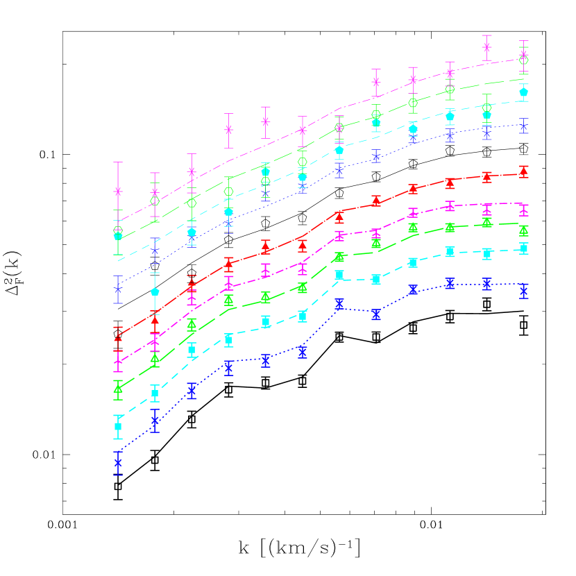
Figure 15: Points with error bars show the observed $P_{F}(k,z)$ from SDSS. Lines show our best fitting model. From bottom to top — z=2.2: black, solid line, open square; z=2.4: blue, dotted line, 4-point star (cross); z=2.6: cyan, dashed line, filled square; z=2.8: green, long-dashed line, open triangle; z=3.0: magenta, dot-dashed line, 3-point star; z=3.2: red, dot-long-dashed line, filled triangle; z=3.4: black, thin solid line, open pentagon; z=3.6: blue, thin dotted line, 5-point star; z=3.8: cyan, thin dashed line, filled pentagon; z=4.0: green, thin long-dashed line, open hexagon; z=4.2: magenta, thin dot-dashed line, 6-point star. Note that the wiggles in the theory curve are caused by SiIII-Ly$\alpha$ cross-correlation.

Figure 16: Points with error bars show the observed $P_{F}(k,z)$ from HIRES (McDonald et al., 2000). Lines show our best fitting model. From bottom to top — z=2.4: black, solid line, open square; z=3.0: blue, dotted line, 4-point star (cross); z=3.9: cyan, dashed line, filled square.

We find $\chi^{2}=185.6$ for the fit, for $\sim 161$ degrees of freedom, which is reasonable (a value this high would occur 9% of the time by chance). The best fit power spectrum parameters are $\Delta^{2}_{L}(k_{p}=0.009~{}{\rm s/km},z_{p}=3.0)=0.452_{-0.057~{}-0.116}^{+0.069~{}+0.141}$ and slope $n_{\rm eff}(k_{p},z_{p})=-2.321_{-0.047~{}-0.102}^{+0.055~{}+0.131}$, where the errors are 1 and 2 $\sigma$ ($\Delta\chi^{2}=1$ and 4 as the parameter of interest is varied while minimizing over the other parameters). The formal (i.e., computed by derivatives of $\chi^{2}$ at the best fit point) correlation coefficient of the errors is $r=0.63$, with $1\sigma$ errors $\pm 0.072$ and $\pm 0.069$ on $\Delta_{L}^{2}(k_{p},z_{p})$ and $n_{\rm eff}(k_{p},z_{p})$, respectively. Figure 17 shows the contours of $\Delta\chi^{2}$ in the $\Delta_{L}^{2}(k_{p},z_{p})-n_{\rm eff}(k_{p},z_{p})$ plane, compared to the contours one would estimate from derivatives at the best fit point.

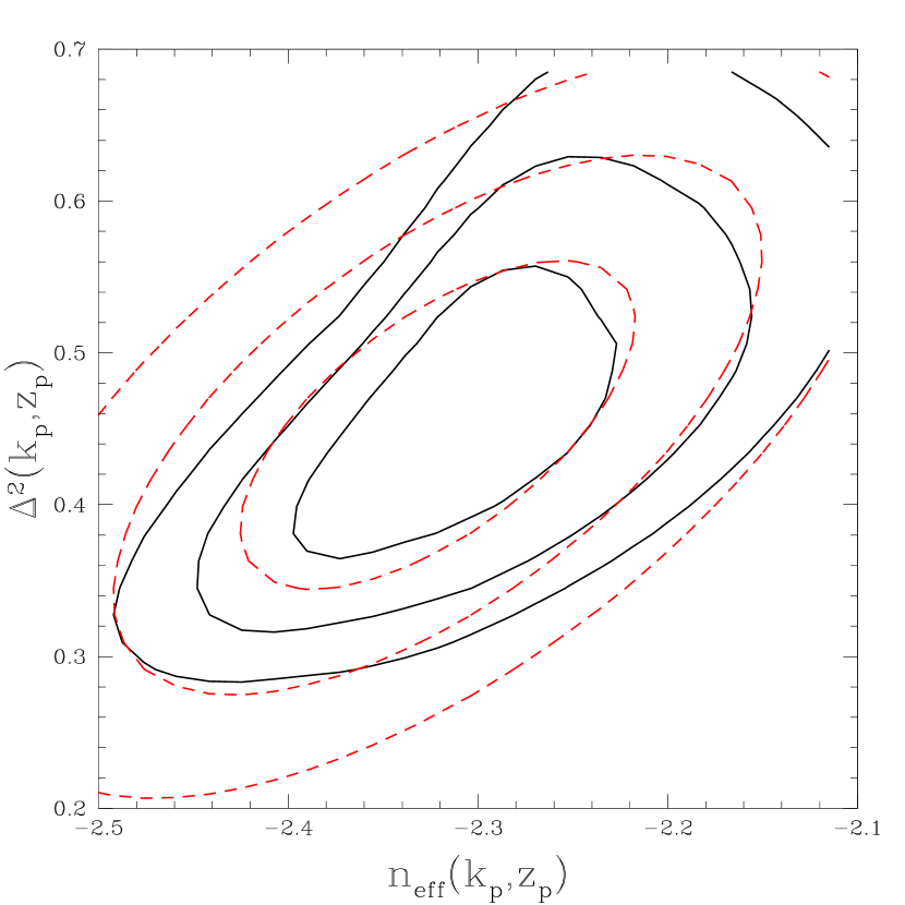
Figure 17: Contours of $\Delta\chi^{2}=2.3$, 6.2, and 11.8, minimized over the other parameters (solid black lines). For comparison, we show the same contours implied using derivatives of $\chi^{2}$ with respect to the parameters at the best fit point (red dashed lines).

We see that, while the local derivative errors are reasonably reflective of the true errors, they are far from perfect. This is not surprising, both because we have various non-Gaussian priors on nuisance parameters, and because the errors generally expand with increasing linear power because of nonlinearities. Fits combining the Ly$\alpha$ forest with other probes of cosmology should use the full contours for maximum accuracy. Figures 18(a,b) show $\Delta\chi^{2}$ for each parameter minimized over the other.

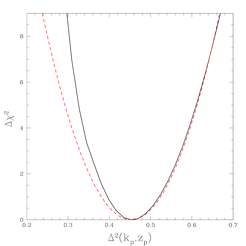
Figure 18: $\Delta\chi^{2}$ as a function of $\Delta_{L}^{2}(k_{p},z_{p})$ (a), and $n_{\rm eff}(k_{p},z_{p})$ (b), minimized over the other parameters (solid black line), or implied by derivatives of $\chi^{2}$ at the best fit point (red dashed lines).

We use these curves to determine the asymmetric errors we quote on the standard result.

For the standard fit, we left $\alpha_{\rm eff}(k_{p},z_{p})=-0.23$, the value in our $\Omega_{m}=0.3$ reference model (with primordial $\alpha=0$). If we include $\alpha_{\rm eff}(k_{p},z_{p})$ as a free parameter, $\chi^{2}$ improves by 1.7, a change that would occur 19% of the time by chance. The best fit value is $\alpha_{\rm eff}(k_{p},z_{p})=-0.135\pm 0.094$. Note that since we have chosen the pivot point $k_{p}=0.009\,{\rm s\,km}^{-1}$ to make the errors on $n_{\rm eff}(k_{p},z_{p})$ and $\alpha_{\rm eff}(k_{p},z_{p})$ approximately independent, the inferred value of $n_{\rm eff}(k_{p},z_{p})$ does not change significantly when $\alpha_{\rm eff}(k_{p},z_{p})$ is varied. In practice, the best fit value of $\Delta_{L}^{2}(k_{p},z_{p})$ does not change either.

We provide an electronic table of $\chi^{2}[\Delta^{2}_{L},n_{\rm eff},\alpha_{\rm eff}]$, a sample of which is shown as Table 1. The table is also available at:
http://www.cita.utoronto.ca/$\sim$pmcdonal/LyaF/lyafchisq.txt .

Table 1: $\chi^{2}[\Delta^{2}_{L},n_{\rm eff},\alpha_{\rm eff}]$

$\Delta_{L}^{2}(k_{p},z_{p})$	$n_{\rm eff}(k_{p},z_{p})$	$\alpha_{\rm eff}(k_{p},z_{p})$	$\chi^{2}$
0.452491	-2.35568	-0.228985	186.798
0.452491	-2.33848	-0.228985	185.872
0.452491	-2.32128	-0.228985	185.595
0.452491	-2.30408	-0.228985	185.821
0.452491	-2.28688	-0.228985	186.22
0.452491	-2.26968	-0.228985	186.723

Note. — $z_{p}=3.0$, $k_{p}=0.009~{}{\rm s/km}$. Points with $\chi^{2}<0$ are either outside the range where we have simulations, or an initial estimate indicated that $\chi^{2}$ would be very high there. The $\alpha_{\rm eff}(k_{p},z_{p})$ dependence is included only to allow more accurate computation of $\chi^{2}$ near $\alpha_{\rm eff}(k_{p},z_{p})=-0.23$, the value for typical $\Lambda$CDM models constrained by WMAP. This table is not intended for models with power spectra qualitatively different in shape from standard $\Lambda$CDM. [The complete version of this table is in the electronic edition of the Journal. The printed edition contains only a sample.]

The table covers the range $0.095<\Delta_{L}^{2}(k_{p},z_{p})<0.685$ in logarithmic steps of $\delta\Delta_{L}/\Delta_{L}=0.06$, covers $-2.665<n_{\rm eff}(k_{p},z_{p})<-1.977$ in steps of 0.017, and $-0.33<\alpha_{\rm eff}(k_{p},z_{p})<-0.13$ in steps of 0.1. A computer code that takes the linear theory power spectrum at $z=3$ and produces $\chi^{2}$ can be found at http://www.cita.utoronto.ca/$\sim$pmcdonal/code.html
under the name “LyaFChiSquared.” This table (or code) will be suitable for joint analyses with the CMB and other observations like those performed in Seljak et al. (2005). It should not be trusted for models where $P_{L}(k)$ is not effectively described by $\Delta_{L}^{2}(k_{p},z_{p})$, $n_{\rm eff}(k_{p},z_{p})$, and $\alpha_{\rm eff}(k_{p},z_{p})$, or models where the values of these parameters deviate substantially from those in typical $\Lambda$CDM-like models, e.g., warm dark matter models (Narayanan et al., 2000) or primordial black hole models (Afshordi et al., 2003) (the code will produce a warning if a suspect power spectrum is input). Our simulation database does contain these models.

3.4 Consistency Checks: Evolution of Slope and Amplitude

If we believe the Universe is effectively Einstein-de Sitter (EdS) in the redshift range we probe then the evolution of $P_{L}(k,z)$ is completely specified (for typical $\Lambda$CDM-like models). Here we test this by measuring the growth factor and the change in the slope of the power spectrum with redshift.

When we allow a power law modification of the growth factor, we find a decrease of 2.8 in $\chi^{2}$, which would occur by chance 9% of the time. The measured growth is $g^{\prime}=1.46\pm 0.29$ (note that $g^{\prime}>1$ means the growth is faster than EdS, the opposite of what one would expect if dark energy was present). We consider this to be an ambiguous result. The deviation from the expectation is not very significant, and the constraint is not tight enough to call this an important consistency check: it rules out gross deviations, but not deviations at the level of the statistical errors on our main result. Still, it would be interesting to explore this further, including additional statistics like the bispectrum, as this method can be one of the few ways to study the presence of dark energy at $z>2$ (Mandelbaum et al., 2003).

When we allow evolution in $n_{\rm eff}$ at fixed comoving $k$ through the parameter $s^{\prime}$ in $n_{\rm eff}[z,k_{\star}(z)]=n_{\rm eff}(k_{p},z_{p})+s^{\prime}(z-z_{p})$, $\chi^{2}$ improves by only 1.8 (probability 18%). The measured value is $s^{\prime}=0.051\pm 0.041$. The size of this error bar is a remarkable, and counterintuitive, result. The evolution of $n_{\rm eff}$ across the redshift range we probe is constrained more tightly than $n_{\rm eff}(k_{p},z_{p})$ itself. In retrospect, this result is not so hard to understand: a substantial part of the error on $n_{\rm eff}(k_{p},z_{p})$ comes from degeneracy with $\Delta_{L}^{2}(k_{p},z_{p})$, which causes the measured values of $n_{\rm eff}$ at different redshifts to move up or down together, depending on the value of $\Delta_{L}^{2}(k_{p},z_{p})$ considered.

So far we have shown three consistency tests [$\alpha_{\rm eff}(k_{p},z_{p})$, $g^{\prime}$, $s^{\prime}$], none of which show compellingly significant deviation from our expectation. Can these be combined to give a significant deviation? The answer is no: when we free all three parameters at the same time, $\chi^{2}$ only decreases by 3.5 relative to the standard fit. This increase occurs by chance 32% of time with 3 free parameters. We can interpret this as a sign that the deviations are statistical in nature and are not consistent with each other in terms of being caused by a common source of systematic error.

To summarize: in this subsection we have demonstrated that we can make precise measurements of the slope of $P_{L}(k_{p},z_{p})$ at multiple redshifts. In the model we use for the interpretation, these values will be tightly correlated, so they can not be combined to give an even better overall measurement, but they act as a stringent discriminator against any physical effect which changes the inferred value of $n_{\rm eff}$ in a way that is not redshift independent. Remarkably, we could detect a redshift dependent effect even if its influence on $n_{\rm eff}$ was smaller than the size of our overall error on $n_{\rm eff}(k_{p},z_{p})$.

3.5 Consistency Checks: Modifications of the Fitting Procedure

Table 2: Effect of modifications of the fitting procedure on the inferred linear power spectrum and its errors

Variant	$\Delta_{L}^{2}$	$n_{\rm eff}$	$\chi^{2}$	$\Delta\chi^{2}$
Standard fit	$0.452\pm 0.072$	$-2.321\pm 0.069$	185.6	0.0
No hydrodynamic corrections	$0.377\pm 0.041$	$-2.284\pm 0.046$	191.8	4.0
Fixed extrapolation	$0.456\pm 0.071$	$-2.303\pm 0.058$	185.9	0.2
Fixed to FULL	$0.453\pm 0.070$	$-2.322\pm 0.063$	185.4	0.0
Fixed to NOSN	$0.435\pm 0.059$	$-2.262\pm 0.054$	187.9	1.9
Fixed to NOMETAL	$0.394\pm 0.048$	$-2.374\pm 0.055$	188.3	1.3
No $L=40\,h^{-1}\,{\rm Mpc}$ simulations	$0.439\pm 0.065$	$-2.328\pm 0.069$	190.0	0.1
$\Omega_{m}=0.4$, HS transfer func.	$0.454\pm 0.074$	$-2.307\pm 0.067$	187.6	0.1
No damping wings (DW)	$0.366\pm 0.042$	$-2.398\pm 0.050$	188.7	1.8
DW power known to 10%	$0.452\pm 0.071$	$-2.321\pm 0.067$	185.6	0.0
Randomly located DW	$0.435\pm 0.070$	$-2.333\pm 0.067$	186.8	0.1
No UVBG fluctuations	$0.446\pm 0.067$	$-2.338\pm 0.049$	187.4	0.2
Strong attenuation UVBG	$0.452\pm 0.072$	$-2.320\pm 0.067$	185.1	0.0
Galaxy-based UVBG	$0.452\pm 0.069$	$-2.346\pm 0.059$	187.4	0.3
$\bar{F}$ errors $\times 2$	$0.452\pm 0.077$	$-2.321\pm 0.071$	184.9	0.0
$\bar{F}$ errors $\times\frac{1}{2}$	$0.455\pm 0.062$	$-2.320\pm 0.066$	188.2	0.0
Fix $\bar{F}$ to best	$0.452\pm 0.030$	$-2.321\pm 0.048$	185.6	0.0
TDR errors $\times 2$	$0.530\pm 0.106$	$-2.299\pm 0.078$	180.4	0.8
TDR errors $\times\frac{1}{2}$	$0.455\pm 0.055$	$-2.305\pm 0.065$	192.0	0.0
Schaye TDR	$0.524\pm 0.059$	$-2.307\pm 0.072$	195.4	1.4
HIRES $P_{F}$ errors $\times 2$	$0.493\pm 0.086$	$-2.276\pm 0.081$	153.8	0.9
HIRES $P_{F}$ errors $\times\frac{1}{2}$	$0.442\pm 0.070$	$-2.335\pm 0.053$	292.1	0.1
SDSS $P_{F}$ errors $\times\frac{1}{2}$	$0.468\pm 0.053$	$-2.301\pm 0.033$	584.3	0.1
Fix nuisance params. to best	$0.452\pm 0.010$	$-2.321\pm 0.012$	185.6	0.0
Inc. Croft/Kim, no back. sub.	$0.355\pm 0.051$	$-2.366\pm 0.054$	313.3	2.9
Include Croft & Kim	$0.408\pm 0.064$	$-2.364\pm 0.063$	215.9	0.4
Drop bad Croft $z$	$0.411\pm 0.064$	$-2.366\pm 0.064$	206.1	0.3
Add Kim only	$0.466\pm 0.082$	$-2.318\pm 0.076$	178.7	0.1
standard w/HIRES back. sub.	$0.503\pm 0.094$	$-2.305\pm 0.081$	161.9	0.6

Note. — $z_{p}=3.0$, $k_{p}=0.009~{}\,{\rm s\,km}^{-1}$.

Our plan in this subsubsection is to investigate the sensitivities of our measurement to various changes in our treatment, to look for potential problems and identify the important areas for future improvement. Table 2 shows the effect of changes in various components of our fitting procedure. For each modification of the procedure, we give the new best fits and errors for $\Delta_{L}^{2}(k_{p},z_{p})$ and $n_{\rm eff}(k_{p},z_{p})$, and $\chi^{2}$ for the new fit, along with $\Delta\chi^{2}$ between the variant and standard best fit power spectrum parameters. We evaluate $\Delta\chi^{2}$ between the two pairs of parameters in the context of both the standard and modified fitting scenarios, and report the smaller change – this method of comparison shows the significance of the modification in a more informative way than simply comparing the change in parameters to the error bars, because it accounts for correlations and deviations from Gaussianity of the errors (we report the smaller $\Delta\chi^{2}$ because when we have two measurements with different sized errors, we do not generally expect the measurement with larger errors to fall within the error contours of the better measurement). Note that, as discussed above, these $\pm 1\sigma$ errors are only intended to be indicative of the true errors, which will not be perfectly Gaussian (in fact, the Gaussian errors are sometimes so bad that we probably should not even report them, as we see, for example, in the standard fit).

Our first modification is to remove the hydrodynamic correction to the HPM prediction of $P_{F}(k,z)$. The change in the result, particularly the amplitude, is significant, although not huge, and $\chi^{2}$ for the fit increases significantly (indicating that the data prefers to have the correction). Note that the reduction in the error bars comes from three things: decreasing the amplitude of the power spectrum always reduces the errors, removing the hydrodynamic correction effectively removes the freedom to modify the large scale power prediction by modifying the form of extrapolation of the correction ($x_{\rm extrap}$ discussed above), and we lose the freedom to choose between the three different forms of galaxy feedback in the hydrodynamic simulations. Note that, as we see from the next line in the Table, the removal of this extrapolation uncertainty (we fix $x_{\rm extrap}=0$) is not what changes the best fit values or $\chi^{2}$, since removing this alone does relatively little.

Next we try using each of the hydrodynamic simulations individually for the correction, rather than letting the fit choose between them. Using FULL has no effect, except to reduce the error bars, because the fit prefers it (the slight reduction in $\chi^{2}$ for FULL versus standard fit is an artifact of the way we impose the boundaries on the simulation-type multipliers). Using the NOSN and NOMETAL simulations leads to small but noticeable changes in the result, although these are disfavored by the increase in $\chi^{2}$.

While our usual method is to use $(40,512)$ simulations for the main $P_{F}(k,z)$ prediction, corrected for limited resolution by comparing (20,512) to (20,256) simulations, we tried performing the fit simply using (20,512) simulations (with the usual form of extrapolation to larger scales). The results are essentially unchanged, although $\chi^{2}$ increases somewhat. This simple test actually rules out a variety of potential problems with the details of our $P_{F}(k,z)$ calculation. One is the possibility that we have statistical errors in the simulation predictions. We have a similar number of each size simulation, which means the (40,512) simulations have 8 times the total volume compared to (20,512). Thus, it would take an unlikely fluke to make the (20,512)-based measurement agree with our (40,512)-based measurement if even the larger simulations had significant statistical error [(20,512) would have even bigger errors]. Another is that substantial systematic errors from the limited size of the $L=40\,h^{-1}\,{\rm Mpc}$ boxes are disfavored, because $L=20\,h^{-1}\,{\rm Mpc}$ should then give an even larger error. Finally, the validity of the resolution correction is confirmed by this test.

Our standard fit is based on the CMBFAST transfer function for the $\Omega_{m}=0.3$ model defined above, and uses this model for the growth factor and Hubble parameter. We tried basing the fit on a model with $\Omega_{m}=0.4$, $\Omega_{b}=0.05$, $h=0.65$, and the Hu & Sugiyama (1996) (HS) transfer function (which is also the model used in the simulations). We expect that this should give results essentially identical to our standard fit. There is no significant change in the fitted parameters, but there is a surprisingly large increase (2.0) in $\chi^{2}$.

Removing the power from high density systems with damping wings has a significant effect on the result, reducing the slope and amplitude and their errors. This is not especially worrisome since the correction that we make can not be very wrong because it is constrained by direct observations of these systems. Reducing our usually assumed 30% error on the size of the effect to 10% does not change the fit results significantly. Using the unrealistic template where the high density systems are randomly distributed in the IGM does not change our fit results although it does increase $\chi^{2}$ by 1.2.

Removing the freedom to include UV background fluctuations in the fit does not change the central values from the fit, but does significantly reduce the error on $n_{\rm eff}(k_{p},z_{p})$, at the cost of increasing $\chi^{2}$ by 1.8. Switching to the UV background fluctuation template for the case where the mean free path of ionizing photons has been arbitrarily halved (this allows a larger maximum effect) gives results very similar to the standard fit. We also tried using the template from McDonald et al. (2005) where Lyman-break galaxies are the source of the ionizing radiation, finding a modest reduction in the error on $n_{\rm eff}(k_{p},z_{p})$, and a small increase in $\chi^{2}$, but ultimately no significant change in our results.

Next we arbitrarily increase or decrease the errors on the observations we use. This is intended to elucidate the importance of the different constraints – the central values that come out of the fits when errors are arbitrarily reduced should not be taken seriously.

It may be surprising that the constraint on $\bar{F}$ actually has little effect on the fit, despite the well-known fact that $P_{F}(k,z)$ is extremely sensitive to $\bar{F}$. The effect of the constraint is so small because the observed power spectrum itself constrains $\bar{F}$ to about $\pm 0.01$, much better than the constraint we have imposed. As we mentioned above, this presents a difficult target for direct measurements of $\bar{F}$, which have to be accurate to this level, including all systematic effects, to be useful. To show that the inclusion of $\bar{F}$ in the fit is important, just not constrained by the external measurements, we repeat the fit with $\bar{F}$ fixed to its best value, so that it doesn’t contribute to the errors on other parameters. We find that the errors on the inferred power spectrum, especially on the amplitude, are reduced dramatically, as one would expect.

The observational constraint we impose on the temperature-density relation does have a noticeable effect. Doubling the errors on the observations of $T_{1.4}$ and $\gamma-1$ leads to a 13% increase in the error on $n_{\rm eff}(k_{p},z_{p})$, and 47% increase in the error on $\Delta_{L}^{2}(k_{p},z_{p})$. Halving the errors reduces the errors on $n_{\rm eff}(k_{p},z_{p})$ and $\Delta_{L}^{2}(k_{p},z_{p})$ by 6% and 24%, respectively. Reassuringly, the best fit values of the parameters do not change very much when the constraints are modified. For comparison, we tried fitting using the much tighter temperature-density relation constraints from Schaye et al. (2000), as re-binned by McDonald et al. (2001): for $z=$(2.46, 3.12, 3.58), $T_{1.4}=(16000\pm 1300,~{}19600\pm 1200,~{}14900\pm 1600)$K and $\gamma-1=(0.34\pm 0.07,~{}0.06\pm 0.07~{},~{}0.22\pm 0.10)$. The fit is not especially good, with $P(>\chi^{2})=3.2$%. The $P_{L}(k_{p},z_{p})$ results change at the $1\sigma$ level, with the error on $\Delta_{L}^{2}(k_{p},z_{p})$ decreasing substantially. The changes in parameter values are consistent with our expectation for random changes based on the change in error bar [e.g., a change in the $\Delta_{L}^{2}(k_{p},z_{p})$ error from $\pm 0.072$ to $\pm 0.053$ implies an expected change $\pm(0.072^{2}-0.053^{2})^{1/2}=\pm 0.049$ in the measured value of $\Delta_{L}^{2}(k_{p},z_{p})$]. There is clearly a lot of room for improvement in the temperature-density relation constraint, which we plan to address with future work.

The HIRES measurement of $P_{F}(k,z)$ that we include is fairly important to the errors on our result, although, again, less important to the central values. Doubling the HIRES errors leads to a 17% increase in the error on $n_{\rm eff}(k_{p},z_{p})$, while halving them reduces this error by 23%. The errors on $\Delta_{L}^{2}(k_{p},z_{p})$ increase by 19% when the HIRES errors are doubled, but remain essentially unchanged when they are halved. Finally, improving the errors on the SDSS $P_{F}(k,z)$ measurement leads to a 26% improvement in the amplitude measurement and 52% in the slope measurement. We are unable to perform a HIRES-only fit without modifications of the procedure because the result is not well constrained to within the region where we have simulations. An SDSS-only fit is better constrained, but still has very large errors, i.e., both high resolution data and SDSS are necessary for good results.

Finally, out of curiosity, we fix all the nuisance parameters to their best fit values, so the only free parameters are $\Delta_{L}^{2}(k_{p},z_{p})$ and $n_{\rm eff}(k_{p},z_{p})$. This tells us how well we could do if we did not need to worry about uncertainties in the Ly$\alpha$ forest model. The resulting errors are $\pm 0.010$ and $\pm 0.012$, respectively.

In summary: While nothing that we have seen necessarily indicates a problem, the importance of some of the corrections indicates that they need to be dealt with carefully in the future, especially if the statistical errors can be reduced. Reducing the statistical errors on the amplitude by more than $\sim 30$% will probably require improvements in more than one of the components of the measurement; however, the $n_{\rm eff}(k_{p},z_{p})$ errors should improve in proportion to the improvement in the SDSS $P_{F}(k,z)$ statistics. The reader should keep in mind that, to keep Table 2 finite, we did not include combinations of changes. An improvement that does not seem useful alone, e.g., reducing the error on the power from damping wings, can become useful if another uncertainty that it is degenerate with is also removed.

3.6 Consistency Checks: Alternative Treatment of High Resolution $P_{F}(k,z)$

Finally, we consider the high resolution $P_{F}(k,z)$ measurements we have not included in our standard fit (Croft et al., 2002; Kim et al., 2004b, a). As we found in McDonald et al. (2004), the fit is poor when these measurements are included: $\chi^{2}=313.3$ for $\sim 250$ degrees of freedom (our usual 161 plus 65 points from Croft et al. (2002) and 24 from Kim et al. (2004a)). In Table 2, the line “Inc. Croft/Kim, no back. sub.” shows this fit (the meaning of “no background subtraction” will become clear shortly). A value of $\chi^{2}$ this high will only occur by chance 0.4% of the time, and the increase of 127.7 in $\chi^{2}$ for 89 additional degrees of freedom is similarly unlikely. Adding Croft et al. (2002) alone increases $\chi^{2}$ by 99.7 ($P(>\chi^{2})=0.4$%), while Kim et al. (2004a) alone increases $\chi^{2}$ by 40.0 ($P(>\chi^{2})=2.1$%). The fit using Kim et al. (2004a) alone is better than it was before the correction of the wavelengths of the bins (Kim et al., 2004b), partially because the ($k=0.0010~{}{\rm s/km}$, $z=2.58$) point with the improbably small error bar is no longer within the $k$ range we are using; however, the fit is still not good enough to be comfortable.

Because we would like to be able to use the additional statistical power of Croft et al. (2002) and Kim et al. (2004b, a), we investigate possible reasons for the bad fits, starting with the statistical error bars. McDonald et al. (2004) pointed out that the Kim et al. (2004a) point at $z=2.58$, $k=0.0010~{}{\rm s/km}$ is inconsistent with the SDSS data, and any reasonable extrapolation of the rest of the Kim et al. (2004a) data (the change in wavelength scale does not change this). It seems likely that the error bar is simply underestimated, possibly because there was not enough data to perform a robust jackknife error estimate. While this point is no longer included in our $k$ range, its existence suggests that the Kim et al. (2004b) errors are not fully reliable. We attempt a correction to the errors based on the following assumptions: the true $P_{F}(k,z)$ should generally increase with decreasing $k$, and the fractional error should also increase (because the data contain fewer modes per bin, and the noise power is insignificant in these spectra). Starting from high $k$, we simply increase the error on each point as necessary to guarantee monotonicity (7 of 24 of the points with $0.0013~{}\,{\rm s\,km}^{-1}<k<0.05~{}\,{\rm s\,km}^{-1}$ have their errors increased). We apply the same adjustment to the Croft et al. (2002) errors (13 of 65 increase), but leave the McDonald et al. (2000) errors unchanged, because McDonald et al. (2000) performed tests of their bootstrap error computation on mock data and already applied a correction based on the results. These error corrections have only a small effect on the results: $\chi^{2}$ decreases to 306.4 (still a poor fit) and the parameter values and error bars change by $<2$% (not shown in Table 2). Unfortunately, the potential problem of poorly determined jackknife error bars seems unlikely to be the cause of our poor fits.

Next we investigate the possibility that the treatment of DLAs in the high resolution data leads to problems. In each of the measurements, DLAs were removed, while our theoretical predictions in the fits assume they are in the data. Note that the error this causes will not be the full size of our damping wing correction (see Figure 11), because much of the correction comes from systems with column density less than $2\times 10^{20}{\rm cm}^{-2}$, which were not necessarily completely removed from any of the high resolution data (some such systems were removed by Kim et al. (2004b), but we do not know how complete this removal was). There is no reason not to be conservative in accounting for this possible error, because the high resolution data is not important to the low $k$ constraints (where damping wings are important), so we simply add a component corresponding to uncertainty at the level of the full amplitude of the damping wing correction to the error covariance matrices of all of the high resolution data (i.e., $C_{ij}^{\prime}=C_{ij}+P_{\rm damp}(k_{i},z)P_{\rm damp}(k_{j},z)$, where $C_{ij}$ is the covariance matrix for redshift bin $z$). The only effect is to decrease $\chi^{2}$ by 3.1 to 303.3 (the power spectrum parameter values and errors change by less than 2% – not shown in Table 2). The treatment of DLAs in the high resolution data does not seem to be important to our goodness of fit.

One of the advances of McDonald et al. (2004) was a careful measurement and subtraction of background power (e.g., from metal absorption), using the $1268<\lambda_{{\rm rest}}<1380$ Å region in the quasar rest frame. Further investigating possible reasons for the bad fits when we include Croft et al. (2002) and Kim et al. (2004b, a), we discovered that the background power measured by Kim et al. (2004b) in their quasar spectra in the restframe wavelength range $1265.67<\lambda<1393.67$ (derivable from their Figure 2) is quite significant for our fits. Kim et al. (2004b) made no correction for this background, but we can make a very rough correction in the following way: First, we read the fractional background from their figure, using the power spectra computed without continuum fitting (F3 in their notation), and finding the numbers: ($k$, $P_{1266,1394}/P_{1026,1203}$) = (0.0011, 0.778), (0.0015, 0.470), (0.0021, 0.233), (0.0030, 0.221), (0.0042, 0.141), (0.0060, 0.090), (0.0085, 0.081), (0.0120, 0.073), (0.0169, 0.090), (0.0239, 0.049), (0.0338, 0.060), and (0.0478, 0.090), where $P_{\lambda_{1},\lambda_{2}}$ means power measured in the rest frame wavelength range $\lambda_{1}<\lambda<\lambda_{2}$ (wavelength in Å, $k$ in s/km). Then, for each $P_{F}(k,z)$ point used in our fit we estimate the absolute background to subtract by multiplying the measured $P_{F}(k,z)$ by this fraction. This background is similar to or larger than that found by McDonald et al. (2004) in SDSS data at the same redshift, depending on the $k$ value and SDSS noise level considered. In particular, on large scales it is much larger. This means that some of the background must be related to the observing and data reduction process rather than metal absorption or quasar continuum power (McDonald et al. (2004) removed only a very small amount of power by dividing the spectra by the mean quasar continuum). For this reason, we will henceforth exclude Kim et al. (2004b) points with $k<0.003~{}\,{\rm s\,km}^{-1}$, where the differences between continuum fitted and not-continuum fitted spectra becomes important, and the disagreement with SDSS data on the background level becomes severe (this same cutoff was suggested by Kim et al. (2004b), although we do not agree that the reason for it is likely to be simple continuum fluctuations). When we perform the background subtraction, we propagate an independent 35% statistical error on the fractional background power for each point (roughly estimated from the error bars on the power measurements in Kim et al. (2004b)), along with the error implied by the uncertainty in the measured power itself. Our estimate of the fractional background using Kim et al. (2004b) in principle applies only to the redshift range in their figure, while the true ratio of background to Ly$\alpha$ forest power will inevitably change with redshift, therefore we allow substantial freedom in the overall amplitude of the subtracted component, equal to 50% of the amplitude at $1\sigma$ (i.e., at 95% confidence, anything from no background to twice the fiducial background is allowed). McDonald et al. (2000) and Croft et al. (2002) present no measurement of the background in their data, although it must be present at some level. We perform the same background subtraction procedure just described on their measurements of $P_{F}(k,z)$, and apply the same $k$ limit, although we note that this procedure is highly dubious because the background may depend on the details of the observations (e.g., the details of sky subtraction).

Using this prescription for the background subtraction from high resolution data, along with the previously described monotonicity constraint on the error bars, and DLA uncertainty, we find $\chi^{2}=215.9$ for $\sim 224$ degrees of freedom, a perfectly good fit. The fitted $P_{L}(k_{p},z_{p})$ parameters change very little relative to our standard fit, and the errors on amplitude and slope both decrease by $\sim 10$% (see the “Include Croft & Kim” entry in Table 2). Figure 19 shows the change of the constraint in the $\Delta_{L}^{2}(k_{p},z_{p})-n_{\rm eff}(k_{p},z_{p})$ plane.

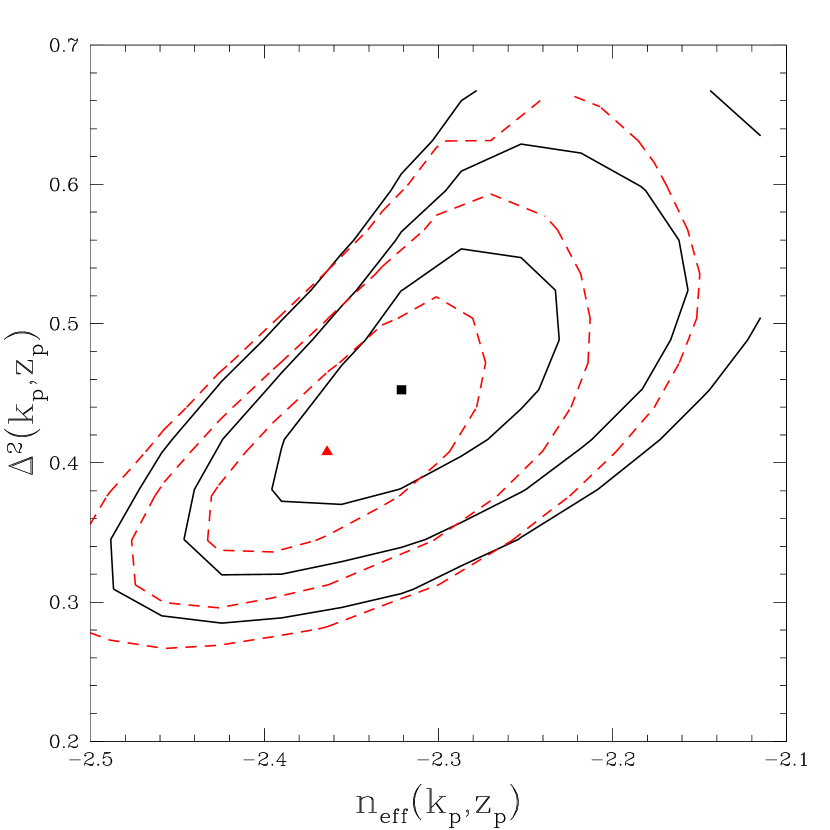
Figure 19: Comparison of standard fit results (black, solid lines and square) to a fit including the Croft et al. (2002) and Kim et al. (2004b, a) high resolution $P_{F}(k,z)$ measurements, with a background correction to all the high resolution measurements (red, dashed lines and triangle). The points show the minimum $\chi^{2}$ while contours show $\Delta\chi^{2}=2.3$, 6.2, and 11.8, minimized over the other parameters.

The change in parameter values falls along the degeneracy direction, making the combined change even less significant than the individual changes might appear to be. Note that changes in parameter values of the size we do see are not a sign of even small systematic disagreement between the data sets – they are perfectly consistent with the expected change whenever independent data is added and extra freedom is allowed in the fit. Table 2 also shows the case where we remove the redshift bin from Croft et al. (2002) that McDonald et al. (2004) identified as suspect. The results do not change much, and $\chi^{2}$ only decreases by 9.7, indicating that we have included enough uncertainty in the covariance matrix to allow this bin to match the other data (this is not to say that we believe simple background is responsible for the strange results in this bin). To explore the relative importance of the different $P_{F}(k,z)$ measurements, we perform the fit without Croft et al. (2002), and using only McDonald et al. (2000) as in our standard fit (but including the DLA error, and the background subtraction – this is “standard w/HIRES back. sub.” in Table 2). The fit with only McDonald et al. (2000) gives a 30% larger amplitude error than our standard fit (and 10% larger $n_{\rm eff}(k_{p},z_{p})$ error), while adding Kim et al. (2004b, a) brings us about half way back to the standard fit (note that one of the significant advances of Kim et al. (2004b) is a $P_{F}(k,z)$ measurement at $z<2.1$, which we are ignoring because it is outside the SDSS range). Adding the Croft et al. (2002) measurement accounts for the rest of the improvement in the errors. None of these variant fits give significantly different central values for the $P_{L}(k_{p},z_{p})$ parameters.

This treatment of the high resolution $P_{F}(k,z)$ measurements is admittedly ad hoc, but nonetheless informative. Some improvement could be made in the $P_{L}(k_{p},z_{p})$ error bars if all of the data could be used. It is clear, however, that an investigation of the background in the spectra actually used in these papers is needed. Ultimately, the results we obtain when all the measurements are included are very similar to our standard results, reassuring us that the cosmological results are not sensitive to the details of the high resolution data.

3.7 Consistency Checks: Nuisance parameter results

Many of the nuisance parameters are interesting in themselves; however, we are hesitant to present their values and error bars from the fits in this paper. Unlike the case of the power spectrum slope and amplitude, we have not checked carefully that the resulting measurements of the other parameters are reliable at the level of precision we could quote. We hope to present complete results for other parameters in the future, but for now their role in our fits should be seen as simply to be descriptors of various forms of uncertainty in the power spectrum extraction. To reassure the reader that the values are reasonable, we give some central values from the fit; however, the errors should be considered to be unknown (which is of course practically equivalent to infinite errors).

Our $\bar{F}(z)$ results are probably the most interesting, because the measurement is quite precise, and the method is completely different from the usual direct measurement. Recall that we parameterized $\bar{F}(z)$ by $\bar{F}(z)=\exp(\ln[\bar{F}(z_{p})][(1+z)/(1+z_{p})]^{\nu_{F}})$. The fitting results are: $\bar{F}(z_{p}=3)=0.69$, $\nu_{F}=3.3$. Unfortunately, we do not know that these $\bar{F}$ numbers are robust estimates of the value of $\left<\exp(-\tau)\right>$ that we should expect to observe directly. We plot this result, along with direct estimates from McDonald et al. (2000) and from the SDSS spectra based on the PCA continuum method described in §2.5 of McDonald et al. (2004), in Figure 20.

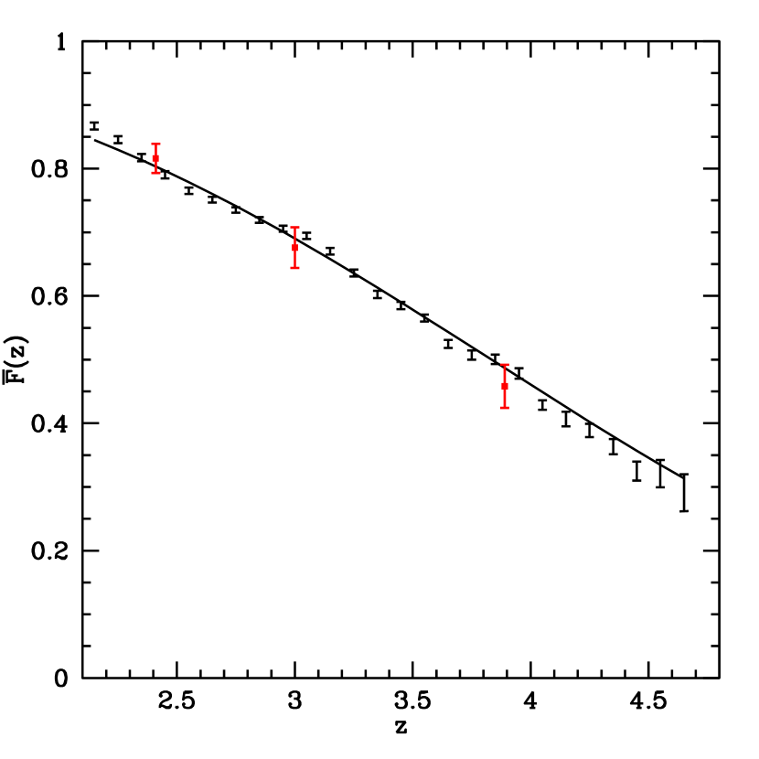
Figure 20: Evolution of the mean transmitted flux fraction, $\bar{F}(z)$. The curve is our indirect measurement from the fit to the power spectrum. The black bars show a direct estimate from the SDSS spectra using a PCA determination of their continua (the overall normalization of these points is arbitrary). The red points with large error bars are from HIRES spectra (McDonald et al., 2000). Intended for qualitative use only – we are not certain that the SDSS measurements are reliable at the level of their error bars, and the errors are correlated.

The PCA measurement is also still preliminary, because we have not been able to rigorously demonstrate convergence to the level of the statistical error bars when increasing the number of eigenvectors used to determine the continuum. Each of these measurements alone may not be perfectly reliable, but together they present a clear, consistent picture of the evolution of the mean absorption (although note that the PCA measurement only constrains the evolution up to a single overall normalizing factor, which has been adjusted to match the other measurements).

The other nuisance parameter results are as follows: The temperature-density relation from the fit is $T_{1.4}=(20000,~{}20000,~{}15000)$K, $\gamma-1=(0.5,~{}0.5,~{}0.1)$ at $z=(2.4,~{}3.0,~{}3.9)$. The reionization/filtering length parameter is at the lower limit of the range we allow (note that this parameter plays a dual role as the final insurance against error caused by limited simulation resolution, as we showed in Figure 2). The SiIII normalization is $f_{\rm SiIII}=0.013$ with redshift evolution poorly constrained. The damping wing power normalization is $A_{\rm damp}=1.0$. The full-physics (FULL) hydrodynamic simulation is favored over the NOMETAL and NOSN simulations. Finally, the presence of significant power from UV background fluctuations is disfavored, but the constraint is weak.

4 Conclusions

Our primary result is the measurement of the amplitude and slope of the linear theory power spectrum at $z\sim 3$ on $\sim 1\,h^{-1}\,{\rm Mpc}$ scales: $\Delta^{2}_{L}(k_{p}=0.009~{}{\rm s/km},z_{p}=3.0)=0.452_{-0.057~{}-0.116}^{+0.069~{}+0.141}$ and $n_{\rm eff}(k_{p},z_{p})=-2.321_{-0.047~{}-0.102}^{+0.055~{}+0.131}$ (these are 1 and 2 $\sigma$ errors, with correlation $r\simeq 0.63$). These were measured as the amplitude and tilt of a CMBFAST power spectrum for a flat $\Lambda$CDM model with $\Omega_{m}=0.3$, $\Omega_{b}=0.04$, and $h=0.7$, and correspond to $\sigma_{8}=0.85$, $n=0.94$ for this model; however, we emphasize that these $\sigma_{8}$ and $n$ numbers aren’t especially meaningful because they are model dependent. The real power of the Ly$\alpha$ forest measurement is achieved when it is combined with the CMB measurements on larger scales (Seljak et al., 2005). If we additionally allow variation in the curvature of the power spectrum, we find $\alpha_{\rm eff}(k_{p},z_{p})=-0.135\pm 0.094$ (the expected value for $\Lambda$CDM models with zero primordial running is $\alpha_{\rm eff}(k_{p},z_{p})\sim-0.23$). As a consistency check, we estimated a power law growth factor, $D(a)\propto a^{g^{\prime}}$, finding $g^{\prime}=1.46\pm 0.29$, consistent with the expectation $g^{\prime}=1.0$. We also estimated the evolution of the inferred slope at a fixed comoving $k$ with redshift, which is expected to be zero, and found $s^{\prime}=dn_{\rm eff}/dz=0.051\pm 0.041$.

The use of the SDSS $P_{F}(k,z)$ measurement (McDonald et al., 2004) represents an improvement over past work. In addition to more data, we have improved the analysis method in several ways: Our method is different from others (with exception of Zaldarriaga et al. (2001)), in that we assume nothing about the dependence of $P_{F}(k,z)$ on $P_{L}(k)$ and other parameters (other than the smoothness assumptions implicit in our interpolation procedure). As a result, our errors on the power spectrum parameters properly incorporate partial degeneracies and correlations with each other and with nuisance parameters such as the mean absorption level $\bar{F}$. We calibrate our HPM simulations using fully hydrodynamic simulations and include non-negligible uncertainty in the calibration, found by comparing simulations with three different versions of the physics. Our most important addition to the Ly$\alpha$ forest model is power contributed by high density systems with damping wings (many of them below the traditional column density of DLAs), as investigated by McDonald et al. (2005). This increases the measured slope and amplitude, and their error bars. We also include the possibility of UV background fluctuations, which turn out to be easy to constrain because their effect changes rapidly with redshift. Note that the systematic error tests in McDonald et al. (2004) show smaller errors than we present here because most of these effects were not included in that analysis.

There is plenty of room for improvement in every aspect of the measurement. The accumulation of SDSS spectra will improve the large-scale $P_{F}(k,z)$ measurement and in turn the errors on $P_{L}$. We showed that improved measurements of $P_{F}(k,z)$ from high resolution data will also help significantly. We only used the HIRES-based measurement of McDonald et al. (2000), because the other existing measurements (Croft et al., 2002; Kim et al., 2004b, a) show signs of problems – they would produce bad $\chi^{2}$ fits if we included them. We investigated the reason for the disagreement and concluded that it is probably the presence of significant unsubtracted background power in the high resolution measurements. After accounting for this in a very rough way, we obtain results consistent with our standard results. For future measurements of the power spectrum (or any Ly$\alpha$ forest statistic), we suggest two steps that can help diagnose problems: (1) The measurement, including the error estimation, should be performed on mock spectra, where the correct result is known, ideally constructed in a format that allows exactly the same analysis code to be applied from end to end. In addition to allowing high precision tests for any bias in the measurement, the ability to produce many complete sets of mock spectra allows a test of the commonly used jackknife or bootstrap errors, which, in particular, may underestimate the errors for small samples of data. (2) The measurement should be performed on the red side of the Ly$\alpha$ emission line and if there is any detection there it should be accounted for (keeping in mind that systematic errors that look small relative to the statistical error on a single data point can still be very significant when they affect many points).

On the theory side, the main improvements to be made are in the size and number of hydrodynamic simulations. The errors on the linear power spectrum $P_{L}$ could be reduced if we did not have to extrapolate as far beyond the scale of the simulation boxes. It might be possible to further reduce the errors if we better understood the causes for the differences between simulations with and without supernova energy feedback and metal cooling. Improving and understanding better the hydrodynamic simulations should be the top priority for the near future. We have not shown that improving the accuracy of the damping wing and UV background fluctuation calculations (McDonald et al., 2005) can improve the $P_{L}$ measurement, but the accuracy can certainly be improved and we suspect that this will become important if other errors can be reduced.

Finally, the measurement of $P_{L}$ can be improved by additional Ly$\alpha$ forest statistics like the bispectrum (Mandelbaum et al., 2003). While we have not found any indication that fundamental issues stand in the way of an even more precise measurement of $P_{L}$ from the Ly$\alpha$ forest, our current analysis does not take advantage of the full statistical power in the data and the challenge of constructing a sufficiently accurate calculational procedure should not be taken lightly.

References

- Abazajian et al. (2004) Abazajian, K., et al. 2004, AJ, 128, 502
- Abazajian et al. (2003) Abazajian, K., et al. 2003, AJ, 126, 2081
- Afshordi et al. (2003) Afshordi, N., McDonald, P., & Spergel, D. N. 2003, ApJ, 594, L71
- Bechtold et al. (1994) Bechtold, J., Crotts, A. P. S., Duncan, R. C., & Fang, Y. 1994, ApJ, 437, L83
- Bernardi et al. (2003) Bernardi, M., et al. 2003, AJ, 125, 32
- Bi et al. (1992) Bi, H. G., Boerner, G., & Chu, Y. 1992, A&A, 266, 1
- Blanton et al. (2003) Blanton, M. R., Lin, H., Lupton, R. H., Maley, F. M., Young, N., Zehavi, I., & Loveday, J. 2003, AJ, 125, 2276
- Cen et al. (1994) Cen, R., Miralda-Escude, J., Ostriker, J. P., & Rauch, M. 1994, ApJ, 437, L9
- Cen et al. (2003) Cen, R., Ostriker, J. P., Prochaska, J. X., & Wolfe, A. M. 2003, ApJ, 598, 741
- Croft (2004) Croft, R. A. C. 2004, ApJ, 610, 642
- Croft et al. (2002) Croft, R. A. C., Weinberg, D. H., Bolte, M., Burles, S., Hernquist, L., Katz, N., Kirkman, D., & Tytler, D. 2002, ApJ, 581, 20
- Croft et al. (1998) Croft, R. A. C., Weinberg, D. H., Katz, N., & Hernquist, L. 1998, ApJ, 495, 44
- Dave et al. (1997) Dave, R., Hernquist, L., Weinberg, D. H., & Katz, N. 1997, ApJ, 477, 21
- Dinshaw et al. (1994) Dinshaw, N., Impey, C. D., Foltz, C. B., Weymann, R. J., & Chaffee, F. H. 1994, ApJ, 437, L87
- Fan et al. (2002) Fan, X., Narayanan, V. K., Strauss, M. A., White, R. L., Becker, R. H., Pentericci, L., & Rix, H. 2002, AJ, 123, 1247
- Fang & White (2004) Fang, T., & White, M. 2004, ApJ, 606, L9
- Fukugita et al. (1996) Fukugita, M., Ichikawa, T., Gunn, J. E., Doi, M., Shimasaku, K., & Schneider, D. P. 1996, AJ, 111, 1748
- Gardner et al. (2001) Gardner, J. P., Katz, N., Hernquist, L., & Weinberg, D. H. 2001, ApJ, 559, 131
- Gnedin et al. (2003) Gnedin, N. Y., et al. 2003, ApJ, 583, 525
- Gnedin & Hamilton (2002) Gnedin, N. Y., & Hamilton, A. J. S. 2002, MNRAS, 334, 107
- Gnedin & Hui (1998) Gnedin, N. Y., & Hui, L. 1998, MNRAS, 296, 44
- Gunn et al. (1998) Gunn, J. E., et al. 1998, AJ, 116, 3040
- Haardt & Madau (1996) Haardt, F., & Madau, P. 1996, ApJ, 461, 20
- Hamilton et al. (1991) Hamilton, A. J. S., Matthews, A., Kumar, P., & Lu, E. 1991, ApJ, 374, L1
- Hernquist et al. (1996) Hernquist, L., Katz, N., Weinberg, D. H., & Jordi, M. 1996, ApJ, 457, L51
- Hogg et al. (2001) Hogg, D. W., Finkbeiner, D. P., Schlegel, D. J., & Gunn, J. E. 2001, AJ, 122, 2129
- Hu & Sugiyama (1996) Hu, W., & Sugiyama, N. 1996, ApJ, 471, 542
- Hui & Gnedin (1997) Hui, L., & Gnedin, N. Y. 1997, MNRAS, 292, 27
- Kim et al. (2004a) Kim, T.-S., Viel, M., Haehnelt, M. G., Carswell, B., & Cristiani, S. 2004a, MNRAS, 351, 1471
- Kim et al. (2004b) Kim, T.-S., Viel, M., Haehnelt, M. G., Carswell, R. F., & Cristiani, S. 2004b, MNRAS, 347, 355
- Lynds (1971) Lynds, R. 1971, ApJ, 164, L73
- Mandelbaum et al. (2003) Mandelbaum, R., McDonald, P., Seljak, U., & Cen, R. 2003, MNRAS, 344, 776
- McDonald (2003) McDonald, P. 2003, ApJ, 585, 34
- McDonald et al. (2001) McDonald, P., Miralda-Escudé, J., Rauch, M., Sargent, W. L. W., Barlow, T. A., & Cen, R. 2001, ApJ, 562, 52
- McDonald et al. (2000) McDonald, P., Miralda-Escudé, J., Rauch, M., Sargent, W. L. W., Barlow, T. A., Cen, R., & Ostriker, J. P. 2000, ApJ, 543, 1
- McDonald et al. (2004) McDonald, P., et al. 2004, ArXiv Astrophysics e-prints, astro-ph/0405013
- McDonald et al. (2005) McDonald, P., Seljak, U., Cen, R., Bode, P., & Ostriker, J. P. 2005, MNRAS, 360, 1471
- Meiksin & White (2001) Meiksin, A., & White, M. 2001, MNRAS, 324, 141
- Meiksin & White (2004) Meiksin, A., & White, M. 2004, MNRAS, 350, 1107
- Miralda-Escude et al. (1996) Miralda-Escude, J., Cen, R., Ostriker, J. P., & Rauch, M. 1996, ApJ, 471, 582
- Nagamine et al. (2004) Nagamine, K., Springel, V., & Hernquist, L. 2004, MNRAS, 348, 421
- Narayanan et al. (2000) Narayanan, V. K., Spergel, D. N., Davé, R., & Ma, C. 2000, ApJ, 543, L103
- O’Shea et al. (2004) O’Shea, B. W., Bryan, G., Bordner, J., Norman, M. L., Abel, T., Harkness, R., & Kritsuk, A. 2004, ArXiv Astrophysics e-prints, astro-ph/0403044
- Péroux et al. (2003a) Péroux, C., Dessauges-Zavadsky, M., D’Odorico, S., Kim, T., & McMahon, R. G. 2003a, MNRAS, 345, 480
- Péroux et al. (2003b) Péroux, C., McMahon, R. G., Storrie-Lombardi, L. J., & Irwin, M. J. 2003b, MNRAS, 346, 1103
- Pier et al. (2003) Pier, J. R., Munn, J. A., Hindsley, R. B., Hennessy, G. S., Kent, S. M., Lupton, R. H., & Ivezić, Ž. 2003, AJ, 125, 1559
- Press et al. (1992) Press, W. H., Teukolsky, S. A., Vetterling, W. T., & Flannery, B. P. 1992, Numerical recipes in C. The art of scientific computing (Cambridge: University Press, —c1992, 2nd ed.)
- Prochaska & Herbert-Fort (2004) Prochaska, J. X., & Herbert-Fort, S. 2004, PASP, 116, 622
- Richards et al. (2002) Richards, G. T., et al. 2002, AJ, 123, 2945
- Ricotti et al. (2000) Ricotti, M., Gnedin, N. Y., & Shull, J. M. 2000, ApJ, 534, 41
- Schaye et al. (2003) Schaye, J., Aguirre, A., Kim, T., Theuns, T., Rauch, M., & Sargent, W. L. W. 2003, ApJ, 596, 768
- Schaye et al. (2000) Schaye, J., Theuns, T., Rauch, M., Efstathiou, G., & Sargent, W. L. W. 2000, MNRAS, 318, 817
- Seljak et al. (2005) Seljak, U., et al. 2005, Phys. Rev. D, 71, 103515
- Seljak et al. (2003) Seljak, U., McDonald, P., & Makarov, A. 2003, MNRAS, 342, L79
- Seljak & Zaldarriaga (1996) Seljak, U., & Zaldarriaga, M. 1996, ApJ, 469, 437
- Smith et al. (1986) Smith, H. E., Cohen, R. D., & Bradley, S. E. 1986, ApJ, 310, 583
- Smith et al. (2002) Smith, J. A., et al. 2002, AJ, 123, 2121
- Stoughton et al. (2002) Stoughton, C., et al. 2002, AJ, 123, 485
- Theuns et al. (1998) Theuns, T., Leonard, A., Efstathiou, G., Pearce, F. R., & Thomas, P. A. 1998, MNRAS, 301, 478
- Trac & Pen (2004) Trac, H., & Pen, U. 2004, New Astronomy, 9, 443
- Tytler et al. (2004) Tytler, D., et al. 2004, ApJ, 617, 1
- Viel et al. (2004a) Viel, M., Haehnelt, M. G., Carswell, R. F., & Kim, T.-S. 2004a, MNRAS, 349, L33
- Viel et al. (2004) Viel, M., Haehnelt, M. G., & Springel, V. 2004, MNRAS, 354, 684
- Viel et al. (2004b) Viel, M., Matarrese, S., Heavens, A., Haehnelt, M. G., Kim, T.-S., Springel, V., & Hernquist, L. 2004b, MNRAS, 347, L26
- Vogt et al. (1994) Vogt, S. S., et al. 1994, in Proc. SPIE Instrumentation in Astronomy VIII, David L. Crawford; Eric R. Craine; Eds., Volume 2198, p. 362, Vol. 2198
- Wolfe et al. (1986) Wolfe, A. M., Turnshek, D. A., Smith, H. E., & Cohen, R. D. 1986, ApJS, 61, 249
- York et al. (2000) York, D. G., et al. 2000, AJ, 120, 1579
- Zaldarriaga et al. (2001) Zaldarriaga, M., Hui, L., & Tegmark, M. 2001, ApJ, 557, 519
- Zaldarriaga et al. (2003) Zaldarriaga, M., Scoccimarro, R., & Hui, L. 2003, ApJ, 590, 1
- Zhang et al. (1995) Zhang, Y., Anninos, P., & Norman, M. L. 1995, ApJ, 453, L57