High Resolution X-ray Spectra of the Brightest OB Stars in the Cygnus OB2 Association

Abstract

The Cygnus OB2 Association contains some of the most luminous OB stars in our Galaxy and the brightest of which are also among the most luminous in X-rays. We obtained a Chandra High Energy Transmission Grating Spectrometer (HETGS) observation centered on Cyg OB2 No. 8a, the most luminous X-ray source in the Association. Although our analysis will focus on the X-ray properties of Cyg OB2 No. 8a, we also present limited analyses of three other OB stars (Cyg OB2 Nos. 5, 9, and 12). Applying standard diagnostic techniques as used in previous studies of early-type stars (e.g., Waldron & Cassinelli 2001), we find that the X-ray properties of Cyg OB2 No. 8a are very similar to those of other OB stars that have been observed using high-resolution X-ray spectroscopy. From analyses of the He-like ion $fir$ emission lines (Mg xi, Si xiii, S xv, and Ar xvii), we derive radial distances of the He-like line emission sources and find that the higher energy ions have their lines form closer to the stellar surface than those of lower ion states. Also these $fir$-inferred radii are found to be consistent with their corresponding X-ray continuum optical depth unity radii. Both of these findings are in agreement with previous O-star studies, and again suggests that anomalously strong shocks or high temperature zones may be present near the base of the wind. The observed X-ray emission line widths ($HWHM\sim 1000$ km s^-1) are also compatible with the observations of other O-star supergiants. Since Cyg OB2 No. 8a is similar in spectral type to $\zeta\$Pup (the only O-star which clearly shows asymmetric X-ray emission line profiles with large blue-shifts), we expected to see similar emission line characteristics. Contrary to other O-star results, the emission lines of Cyg OB2 No. 8a show a large range in line centroid shifts ($\sim$ -800 to +250 km s^-1). However, we argue that most of the largest shifts may be unreliable, and the resultant range in shifts is much less than those observed in $\zeta\$Pup. Although there is one exception, the H-like Mg xii line which shows a blue-shift of -550 km s^-1, there are problems associated with trying to understand the nature of this isolated large blue-shifted line. To address the degree of asymmetry in these line profiles, we present Gaussian best-fit line profile model spectra from $\zeta\$Pup to illustrate the expected asymmetry signature in the $\chi^{2}$ residuals. Comparisons of the Cyg OB2 No. 8a best-fit line profile residuals with those of $\zeta\$Pup suggest that there are no indications of any statistical significant asymmetries in these line profiles. Both the line shift characteristics and lack of line asymmetries are very puzzling results. Given the very high mass loss rate of Cyg OB2 No. 8a (approximately five times larger than previous Chandra observed O supergiants), the emission lines from this star should display a significant level of line asymmetry and blue-shifts as compared to other OB stars. We also discuss the implications of our results in light of the fact that Cyg OB2 No. 8a is a member of a rather tight stellar cluster, and shocks could arise at interfaces with the winds of these other stars.

1 Introduction

The Cygnus OB2 association (Cyg OB2) is significant in the history of stellar X-ray astronomy in that Einstein Observatory observations of Cyg OB2 were the first to show that early-type stars are X-ray sources (Harnden et al. 1979). Cassinelli & Olson (1979) predicted that OB stars should be X-ray sources based on the superionization stages seen in UV spectra, and suggested that the X-rays arose from a coronal region at the base of a cool wind. Based on their Cyg OB2 X-ray observations, Harnden et al. found that the coronal plus cool wind model predicted too low a flux of soft X-rays owing to the expected attenuation by the overlying wind, and they suggested that the X-rays come from a distribution of shocks in the stellar wind. Lucy & White (1980) developed the first shock model for these stars, and the concept of embedded shocks has remained the prevailing picture for the origin of OB stellar X-rays. The X-ray observations of Cyg OB2 using Einstein (Harden et al. 1979), ROSAT (Waldron et al. 1998), and ASCA (Kitamoto & Mukai 1996) found that the brightest stars in this association have significantly larger X-ray luminosities in comparison with other OB stars. However, the Cyg OB2 stars have larger bolometric luminosities, and the X-ray to bolometric luminosity ratio is in line with that of other OB stars (i.e., with an observed $L_{x}/L_{bol}$ $\sim 10^{-7}$; Berghöfer et al. 1997). Among the early type stars in Cyg OB2, star No. 8a is particularly interesting because it is one of the most X-ray luminous O-stars ($L_{x}=1.5\times 10^{33}$ ergs  s^-1), and because its fast wind has a large mass loss rate, ($\dot{M}$$>10^{-5}$ $M_{\odot}\,$yr^-1) which is almost as large as that of Wolf-Rayet stars. In addition, all of the four brightest stars in Cyg OB2 ( Nos. 5, 8a, 9, & 12) are also know to be variable, non-thermal radio sources (Abbott, Bieging, & Churchwell 1981; Bieging, Abbott, & Churchwell 1989).

Since this association contains some of the most luminous stars in our galaxy (Cyg OB2 Nos. 9 and 12), it has been the focus of many massive star studies. For example, Knödlseder (2000), using the 2MASS near infrared survey data, analyzed the extent and population properties of Cyg OB2 and proposed that it should be reclassified as a “young globular cluster” instead of an OB Association. As he points out, this association is providing opportunities to study the upper end of the main sequence of stars in a rather dense population. The subject of massive star clusters has recently become even more important owing to the well received idea that massive stars are formed by mergers in tight clusters (Bonnell & Bate 2002; Bonnell, Vine, & Bate 2004). The core of Cyg OB2 might originally have been such a region.

The rapidly expanding stellar winds from OB stars are often considered one of the most unexpected and important discoveries of NASA’s early space program (Snow & Morton 1977). Over the years we have learned a great deal about the wind driving mechanisms and wind properties (see Lamers & Cassinelli 1999). However, it is the nature of the processes that lead to shocks and X-ray emission that is still unclear and is currently the center of attention in OB stellar wind research. As shown by recent studies (Waldron & Cassinelli 2001; Cassinelli et al. 2001; Miller et al. 2002), the resolving power of the Chandra High Energy Transmission Grating Spectrometer (HETGS) can provide the critical information required to help us understand these processes. For the first time, astronomers are observing spectrally resolved X-ray line profiles from OB stars. In particular, tight line complexes like the forbidden, intercombination, and resonance ($fir$) lines of He-like ions are spectrally resolved by the HETGS. There are relatively few OB stars that will probably be observed with Chandra at this high spectral resolution since large exposure times are required, so it is important to glean as much information as possible from targets such as the Cyg OB2 stars.

Before the launch of Chandra there was only indirect evidence for a shocked-wind origin for OB stellar X-rays. These include: a) the lack of sufficient oxygen K-shell absorption in previous lower resolution X-ray spectra (Cassinelli et al. 1981; Cassinelli & Swank 1983; Corcoran et al. 1993); b) the consistency of observed O vi UV P-Cygni line profiles with an embedded X-ray source (MacFarlane et al. 1993); and c) theoretical wind instability studies (Lucy & White 1980; Owocki, Castor, & Rybicki 1988; Cooper 1994; Feldmeier 1995). In our Chandra observations of $\zeta\$Ori (Waldron & Cassinelli 2001), $\zeta\$Pup (Cassinelli et al. 2001), and $\delta\$Ori (Miller et al. 2002), we found that far more precise information regarding the location of the X-ray sources could be determined from analyses of the He-like ion $fir$ lines (e.g., O vii, Ne ix, Mg xi, Si xiii, S xv). In particular, the $f/i$ line ratio has long been used as an electron density diagnostic for solar-like plasmas. However, for the case of OB stars, it is the large mean intensity of UV/EUV photons, and not the density of electrons, that determines the relevant population levels, as discussed by Blumenthal, Drake, & Tucker (1972). The $f/i$ line ratio can be used to derive the geometrical dilution factor of the stellar radiation field, and this allows us to extract the distance between the $fir$ line formation region and the photospheric source of UV/EUV radiation. We call $R_{fir}$ the $fir$-inferred radius of the line formation region derived from the He-like ions.

Our analyses indicate that the derived $R_{fir}$ for the O-stars correspond reasonably well with their respective X-ray continuum optical depth unity wind radii as summarized by Waldron & Cassinelli (2002). This correspondence in radii indicates that the X-rays source regions are distributed throughout the wind from just above the photosphere out to approximately 10 $R_{*}$. However, this does not mean that the entire wind is emitting X-rays, but rather that there are sources of hot X-ray emitting material embedded in much cooler gas at all levels of the wind. In fact, the X-rays must be arising from only a small fraction of the matter in the wind. For example, by assuming that the total observed X-ray emission is approximately equal to the total intrinsic X-ray emission, the resultant emission measures are found to be 4 to 5 orders of magnitude smaller than the total wind emission measure (Cassinelli et al. 1981; Kahn et al. 2001). This small fraction of very hot gas is probably in the form of shock fragments and filaments in the clumpy and turbulent outflows.

Although the results seem to support the idea that O-star X-rays arise in shock fragments embedded in stellar winds, two interesting problems have emerged. First, the lines of the highest ion stages arise deep in the flow and require shock jumps, $\Delta v$, that are larger than the local wind speed (Waldron & Cassinelli 2001). Several suggestions have been offered: fast ejecta emerge from sub-photosphere regions (Feldmeier, Shlosman, & Hamann 2002); in-fall of stalled wind material in the form of clumps (Howk et al. 2000); or confinement of anomalously hot gas in magnetic loops (Cassinelli & Swank 1983; Waldron & Cassinelli 2001; Schulz et al. 2003). Second, the observed X-ray line profile shapes do not conform to pre-launch expectations. As expected from an expanding distribution of X-ray sources embedded in a stellar wind, the observed X-ray line profiles from O-stars with massive winds show a large range in broadness with $HWHM$ of $\sim 200$ to $1500$ km s^-1. However, with the exception of one star, the line centroids are not Doppler blue-shifted. Such a shifting or skewing of line profiles to shorter wavelengths was expected, as predicted by MacFarlane et al. (1991) as an effect of X-ray absorption by the wind. The X-rays from the shocks on the back-side (red-shifted) part of the wind should be more strongly attenuated than the X-rays from the wind material on the front-side moving towards the observer (blue-shifted). The O4f star $\zeta\$Pup (the only early O-star spectral type observed so far) is currently the only star thus far which clearly shows the expected blue-ward shifted skewed X-ray line profiles, so it is of special interest to see if the O5.5 I(f) star Cyg OB2 No. 8a shows similar line properties.

The lack of Doppler blue-shifted lines in nearly all OB stars is without a doubt the most unexpected result obtained by Chandra observations. Although the simplest explanation for this dilemma is to say that all the X-ray emission is located at radii where the wind attenuation of the receding X-ray emission is negligible, the problem is that these radii are found to be much larger (order of magnitude) than the $fir$-inferred radii (Waldron & Cassinelli 2001). Even for the largest observed $R_{fir}$, the wind density is still large enough such that most of the red-shifted line emission should be attenuated, and blue-shifted, asymmetric line profiles should still be observed. A possible explanation is that the winds are especially porous or ‘clumped’ which would allow significantly more red-shifted X-rays from the back side to propagate through the stellar wind. For example, the winds may have small filling factors of absorbing material as would be the case for highly clumped winds. The idea of highly clumped winds in OB stars is gaining support. Waldron & Cassinelli (2001) presented the first attempt to fit HETGS line profiles with a wind distributed X-ray source model and concluded that the wind absorption had to be significantly reduced either by large reductions in the mass loss rate or the X-rays are distributed in a highly non-symmetric wind (i.e., clumps). Even for the only star showing clear blue-shifts and asymmetric lines (i.e., $\zeta\$Pup), Kramer, Cohen & Owocki (2003) also found that significant reductions in the wind absorption were required to explain these profiles. Howk et al. (2000) present arguments that the X-rays from OB stars are formed in bow shocks around clumps in the winds. The fact that shocks lead to highly compressed regions that may be Rayleigh-Taylor unstable led Feldmeier, Oskinova, & Hamann (2003) to consider the effects of absorption in fragmented winds. They show that the fragmented nature of a wind allows the X-rays to escape from much deeper in the wind than would be the case for smooth, un-clumped winds. Interestingly, the idea that clumps could be important for the formation and transmission of X-rays in OB stellar winds can be traced back to Lucy & White (1980) and their first alternative model to the coronal idea for X-ray formation. The Lucy & White (1980) model had fast clumps being driven by radiation forces through the ambient wind and this would produce frontal (or forward facing) bow shocks. The more recent models such as Howk et al. (2000) have the fast winds colliding with slower clumps and these produce reverse shocks. Reverse shocks also tend to be the dominant source of X-rays in one-dimensional hydrodynamic models (e.g., Feldmeier 1995).

Although wind clumping appears to be a possible answer to the blue-shift problem, the clumps introduce a dilemma with regards the $f/i$ line ratio analysis results. Since a highly clumped wind implies that the mass loss rates reported for these stars are actually overestimates of their true values, then the relationship between the $fir$-inferred radii and X-ray continuum optical depth unity radii is no longer correct, and we are then faced with a new problem of understanding the significance of this observed correlation. In addition, whatever level of wind clumping is required to explain the X-rays must also be consistent with the observational constraints established at other wavelength bands (e.g., UV, IR, & radio). Again, historically, it is interesting to note that the main argument against the base coronal model of Cassinelli & Olson (1979) and Waldron (1984) was that the X-ray absorption was too large to see any X-rays arising from regions near the photosphere.

Our primary target is the brightest X-ray source, Cyg OB2 No. 8a, and will be the focus of our discussion, but some information about the other OB stars will be presented. In Section 2 we discuss the data reduction and present the HETG spectra of four Cyg OB2 stars. Our observational analyses for obtaining line emission characteristics and the distribution of the X-ray emission are presented in Section 3. The conclusions are discussed in Section 4.

2 The Chandra Observations of Cyg OB2

2.1 Data Reduction

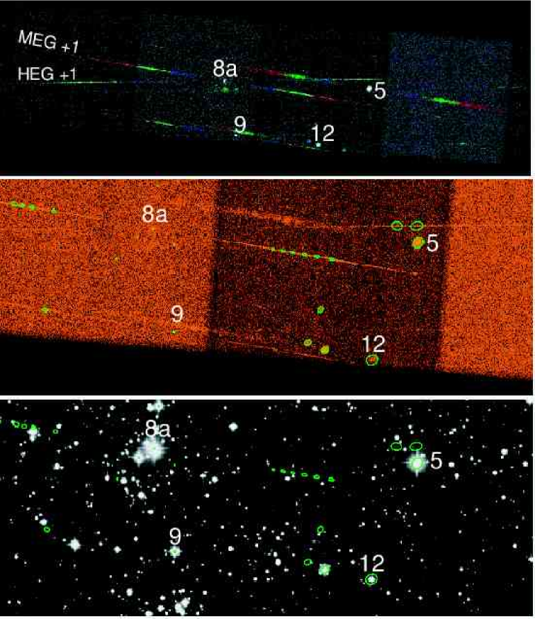
Figure 1: This shows a “true-color” X-ray image showing the Chandra spectra of the central region of Cyg OB2. For all images, North is up. Photons are color-coded according to the following scheme: Red $<1.5$ keV, Green = $1.5-2.5$ keV, and Blue = $2.5-8$ keV. The middle panel shows the ACIS-I focal plane image with the sources (shown by green circles) found using the CIAO tool TGDETECT. The bottom panel shows the same regions on a Digital Sky Survey of the same region. Although some of these detected sources correspond to stars in the Cyg OB2 Association, several circled regions shown in the middle and bottom panels are not actual X-ray sources. For example, the straight rows of circled regions along the MEG spectrum on either side of Cyg OB2 No. 8a and a few other circled regions (as determined by the automatic source detection routine) are simply marking the locations of bright emission lines in the dispersed X-ray spectra of the four brightest stars.

Observations were taken with the Chandra X-ray Observatory using the ACIS-S CCD’s with the HETGS in the optical path. The observation of the Cyg OB2 association [Observation Identification Number (ObsID) 2572] began on July 31, 2002 at 1^h 51^m 04^s UT with an exposure time of approximately 65.12 ks. The spacecraft aim point was chosen to place the primary target, cluster member Cyg OB2 No. 8a, in the center of the focal plane. This gives us a sharp zeroth order image and the highest energy resolution spectrum possible for this star. During this observation, the spacecraft aspect angle was chosen to allow recovery of the dispersed spectra of the three other stars, Cyg OB2 Nos. 5, 9, 12. A “true-color” image constructed from the data is displayed in Figure 1 which shows the typical rainbow colors of the High Energy Grating (HEG) and Medium Energy Grating (MEG) dispersed spectra (e.g., Figure 8.1 in the Chandra Proposers Observatory Guide, CXC 2002).

The CIAO tool TGDETECT was used to locate X-ray sources in the focal plane image. The sources found are displayed in the middle frame of Figure 1. A comparison with the Digital Sky survey image of the same region immediately allows the four brightest sources to be identified with Cyg OB2 Nos. 8a, 5, 9, and 12. Table 1 lists the adopted stellar parameters for these four stars. Although a number of other faint stellar sources are detected, this paper concentrates on what can be learned from the four HETGS dispersed spectra obtained during this observation, primarily Cyg OB2 No. 8a. Since all four stars have large ISM absorption column densities (see Table 1) the extracted spectra reveal essentially no information for $\lambda>12$ Å. The observed count rates for Cyg OB2 No. 8a are 0.102 (MEG$\pm$1) and 0.044 (HEG$\pm$1). The only other spectrum strong enough to allow detailed analyses of a few strong lines is Cyg OB2 No. 9 which has count rates of 0.022 (MEG$\pm$1) and 0.007 (HEG$\pm$1).

The intrinsic energy resolution of the ACIS-S CCDs act as an effective cross dispersion, so individual photon events in the dispersed spectra can be assigned relatively unambiguously to the correct source. When extracting and calibrating the dispersed spectra for these four bright point sources, the following issues needed to be kept in mind:

• Because these stars are off-axis, the High Resolution Mirror Assembly (HRMA) effective area is somewhat less and the line-response function for Cyg OB2 No. 5, 9, and 12 is somewhat broader (e.g., Figure 8.23 of the CPOG, CXC 2002). In particular, note the direct image of star Cyg OB2 No. 5. It is so far off the optical axis of the HRMA that its zeroth order image is considerably broadened, greatly reducing the resolution of the dispersed spectrum (See pp. 41-50 and 187-190 of CXC 2002).

• As our primary target, the direct image of Cyg OB2 No. 8a is near the center of the ACIS-I CCD array. Its whole spectrum for the HEG and MEG fell on light-sensitive areas of ACIS-S. Because of its location, this is also the case for Cyg OB2 No. 5. However, for stars Cyg OB2 Nos. 9 and 12, their positions near the edge of the chip array means that part of their MEG -1 and HEG +1 spectra fell outside the light-sensitive area of the chip, resulting in lower effective areas at longer wavelengths.

• When dealing with an observation containing multiple X-ray sources, such as this one, it is theoretically possible for an individual photon event to be at the correct focal plane position and energy for more than one source (Figure 8.28, CXC 2002). If such a spatial-spectral “collision” occurs, the identification of a single source for that particular photon would become ambiguous. This might occur when a MEG spectrum of one source overlaps a HEG spectrum of another source (see the overlap between the spectra of stars Cyg OB2 Nos. 8a and 5 in our observation). To assess how this problem might effect this observation, we independently constructed photon event lists for the spectra of the four brightest X-ray sources in the field: Cyg OB2 Nos. 5, 8a, 9, and 12. We then examined the resulting photon event lists, checking for any individual photon events which occurred in more than one event list. No such photons were found, indicating that each of the extracted spectra are basically free from contamination by the other sources in the field. In each case, the observed similarity of the positive and negative orders (when both were available) for each source also confirmed that no such contamination occurred.

• The direct images of Cyg OB2 Nos. 5 and 12 did not fall on chip S3, the usual pointing direction. The default chip set in the CIAO tool MKGARF had to be reset to include chip S2 to prevent the erroneous calculation of zero effective area for the portions of the HEG+1 and MEG+1 order spectra which fell on that chip.

High-resolution spectra derived from HETG-ACIS-S naturally have an extremely low background because the intrinsic energy discrimination of the ACIS-S effectively acts as a cross dispersion. This not only allows photon events at a specific position along a spectrum to be sorted to the correct order, but also causes most background events (which have incorrect energies for a given location) to be rejected.

2.2 HETG Spectra of the Cyg OB2 Stars

To survey the dispersed spectral data for the four bright stars, we co-added the positive and negative first order spectra of each of the four stars (the $2^{nd}$ and $3^{rd}$ order spectra were found to have too few counts to make any significant contributions). The HEG and MEG $\pm$1 count spectra for Cyg OB2 No. 8a are shown in Figure 2, and Figure 3 shows the MEG $\pm$1 spectrum of Cyg OB2 No. 9. Unlike other O-star spectra, the spectra of these two stars are noticeably dominated by only two strong lines, the H-like Si xiv line and the He-like Si xiii $fir$ lines. The source of this difference from other O-stars is related to the greater high energy emission associated with these stars, and the much larger ISM extinction. In addition, the Cyg OB2 No. 8a spectra reveals several higher energy ionic line emissions (e.g., Ar xvii, Ca xix, Fe xx, Fe xxii, Fe xxiii, Fe xxiv, & possibility Fe xxv). Although Fe xx, Fe xxii, Fe xxiii, and Fe xxiv were seen in our HETGS observation of $\delta\$Ori (Miller et al. 2002), none of these ionic species were seen in our other O-star supergiant HETGS observations.

The other two stars, Cyg OB2 Nos. 5 & 12, have much weaker count spectra. However, we can provide a comparison of all four stars by displaying their associated MEG$\pm 1$ flux spectra in Figure 4 which provides us with a first order approximation of the X-ray line fluxes for comparisons among these four stars. For each star, a custom Ancillary Response File (ARF) and a Redistribution Matrix File (RMF) were generated using the standard CIAO routines, and the flux spectra were obtained by multiplying the count spectra by the bin energy and dividing by the associated ARF and exposure time. Even though line-shape parameters cannot be recovered from many lines in these spectra, the fact that individual lines are resolved in the dispersed spectra still opens up avenues of investigation which are not possible with CCD-resolution spectra such as a non-grating ACIS-S observation. However, as discussed in Section 2.1, artificial line broadening can occur for off-axis sources due to variations in the instrumental line spread function. For example, some of the lines in the spectrum of Cyg OB2 No. 5 appear much wider than seen in the other stars, but this appearance is most likely caused by the large off-axis location of the source.

3 Observational Analysis

3.1 Measuring the X-ray Emission Line Properties

Since the X-ray line emission profiles from OB stars are very broad ($HWHM~{}\sim 1000$ km s^-1), early-type stars are among the few classes of X-ray sources for which line shapes can be resolved using the HETGS. This capability allows us to study detailed line formation processes that we suspect are operating in these stars. Although the currently accepted scenario is that a distribution of stellar wind shocks are responsible for the observed X-ray emission, Chandra observational results are raising several key issues concerning the exact nature of this distribution, including the possibility that not all of the X-ray emission arises from the stellar wind.

A key parameter in determining the structure of an X-ray line profile from a wind distribution of sources is the stellar wind column density scale factor which is proportional to ${\hbox{$\dot{M}$}}/(\hbox{$v_{\infty}$}\hbox{$R_{*}$})$ (see Waldron et al. 1998). Since the mass loss rate of Cyg OB2 No. 8a is about 5 times greater than $\zeta\$Pup (the only O-star showing well defined blue-shifted lines), we find that this column density scale factor is $\sim 3$ times larger than for $\zeta\$Pup. Hence, well pronounced blue-shifts accompanied by highly asymmetric line profiles are expected.

3.1.1 Line Fitting Procedure

We derive X-ray emission line properties using a relatively simple line fitting procedure. We assume that all emission lines can be represented by Gaussian line profiles superimposed on an underlying bremsstrahlung continuum. The line emissivities and rest wavelengths are obtained from the Astrophysical Plasma Emission Code and Database (APEC and APED; Smith & Brickhouse 2000). For each line, the free parameters are the centroid shift velocity ($V_{S}$), the $HWHM$ velocity, and the line normalization strength (i.e., the line emission measure, $EM_{X}$). Since we are only concerned with the total flux within a line, we find that our fits are essentially independent of our choice of the continuum temperature. For all fits we assume a continuum temperature of 10 MK. In this paper, we concentrate only on the H-like and He-like lines. For each individual line or line complex, we define a wavelength region large enough to cover the emission lines and provide a good representation of the underlying continuum. In many cases, the defined wavelength region may include other weaker lines, and to ensure we obtain the best estimate of the flux in the strongest line and continuum, we include any lines which are likely to contribute to the observed emission. When fitting a region with multiple lines, we always assume that they all have the same $V_{S}$ and $HWHM$, and only the line and continuum $EM_{X}$ will be different. This approach is clearly justified for the He-like $fir$ lines since all three of these lines must be formed under the same conditions, and the only parameter that could be different is the normalization of each line. Although all H-like lines and the He-like $i$ lines are doublets, their separations are much less than the resolving capabilities of both the MEG and HEG, so the lines are represented by only one Gaussian.

We use the standard $\chi^{2}$ statistics to determine a goodness of fit. The quoted best-fit values for $V_{S}$ and $HWHM$ represent averages of their respective $\chi^{2}$ 90% confidence region range for each parameter, and the quoted errors are associated with the difference from the average. These errors do not include the associated MEG and HEG instrumental wavelength uncertainties (e.g., see Table 8.1, CXC 2002). The line flux errors are determined by the total counting statistics within the line. Each model line is folded through the HETGS instrumental response functions (ARF and RMF) as determined for each star, and the best fit values are extracted. To maintain consistency in fitting the MEG and HEG lines, the $\chi^{2}$ statistics are based on fitting a bin size of 0.01 Å for both the MEG and HEG which is approximately equal to the wavelength resolution limit of the HEG instrument (0.012 Å; CXC 2002). Because the MEG and HEG have different line response functions, we analyzed them separately. It should be noted that the fits resulting from the two instruments are consistent with one another, especially for the lines with the highest signal-to-noise ratio (S/N).

3.1.2 Determining the Degree of Line Asymmetry

We test the degree of line asymmetry by analyzing the distribution of the $\chi^{2}$ residuals. For example, suppose we have a triangular shaped emission line (e.g., MacFarlane et al. 1991) with the peak of the triangle located blue-ward from the rest wavelength and the line emission steadily drops from this peak value to zero towards the red-ward side of the line (there is no emission blue-ward of the peak). By attempting to fit this line with a model Gaussian line profile, we expect two characteristic features to emerge: 1) the Gaussian fit will underestimate the line centroid shift, and; 2) the residuals blue-ward of the Gaussian best fit line centroid shift velocity will be positive (model underestimates the data), whereas, red-ward from this centroid shift velocity, the residuals will be negative (model overestimates the data). Hence, a clear residual signature is expected if there is asymmetry in an observed emission line.

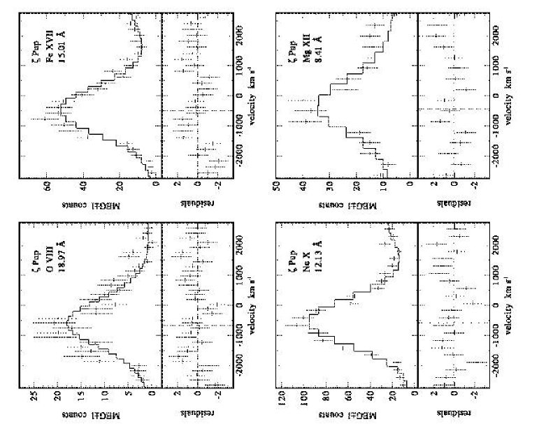
Figure 5: Shows comparisons of the four strongest Zeta Pup H-like best-fit line model spectra (solid-line) with their corresponding observed $MEG\pm 1$ count spectra and their associated residuals. The horizontal axis is expressed as the velocity shift relative to the rest wavelength of the line. The vertical dashed-lines in the residual plots represent the best-fit line centroid shift velocities ($V_{S}$). In order to obtain reliable flux measurements of the line and continuum emissions for Ne x, the input model spectrum included the weaker Fe xvii($\sim 12.26$ Å) located at $\sim 3200$ km s^-1. The bin size is 0.01 Å.

To test this hypothesis, Figure 5 shows the Gaussian best-fit models for the four strongest H-like emission lines of $\zeta\$Pup  which is known to have large blue-shifts and asymmetric line profiles (Cassinelli et al. 2001). The expected residual signature is clearly evident in the Fe xvii and O viii lines, and possibility in the Ne x line. The Mg xii line appears to have no line asymmetry based on our residual analysis. Hence, we will use these $\zeta\$Pup line fit residual signatures as our benchmark for establishing the degree of X-ray emission line asymmetries in our Cyg OB2 No. 8a line profiles. Note that this approach cannot be applied to regions of line overlap such as $fir$ line complexes.

3.1.3 Best-Fit Line Emission Characteristics

We apply our line fitting procedure to the four H-like and four He-like X-ray emission lines of Cyg OB2 No. 8a. The results of our fits are given Table 2 which lists the ion, rest wavelength, observed line flux, $V_{S}$, $HWHM$, $EM_{X}$, the X-ray temperature ($T_{L}$) range where the line emissivity is within 75% of its expected maximum value, and the reduced $\chi^{2}$ . The $EM_{X}$ are derived as explained by Kahn et al. (2001), including ISM absorption corrections, and their errors are based on the differences associated with the range in emissivities as determined by the range in $T_{L}$. In Table 2, the fluxes for the He-like ion $fir$ lines represents the total flux from all three lines, but the listed $EM_{X}$ corresponds to the $EM_{X}$ of the $r$ line only. One has to be careful in their interpretation of $EM_{X}$ derived from the $i$ and $f$ lines since the emissivities used to derive these quantities have not been corrected for either density and/or UV effects. Hence, the $r$ line $EM_{X}$ represents the most reasonable estimate since it is essentially unaffected by these density and UV effects. The individual fluxes from the three $fir$ lines are given in Table 3 (see $fir$ discussion in Sec. 3.2).

The MEG and HEG H-like X-ray line fits and $\chi^{2}$ residuals are shown respectively in Figure 6 and Figure 7. Correspondingly, the MEG and HEG He-like X-ray line fits are shown respectively in Figure 8 and Figure 9. Although the line fits indicate a tendency for blue-shifted lines (see $V_{S}$ in Table 2), these shifts are smaller than those of $\zeta\$Pup, which have an average blue-shift of $\sim-500$ km s^-1 (Cassinelli et al. 2001). Furthermore, these line shifts are significantly smaller than expected as discussed in Section 3.1.1, and most of these line shifts are similar to other O-star results which also show minimal or no blue-shifts. However, for a few lines, large blue-shifts are indicated (see Sec. 3.1.4). The expected line broadness seen in O-star spectra is also present in the four brightest Cyg OB2 OB stars. Our detailed analyses of Cyg OB2 No. 8a indicates that all H-like and He-like lines have $HWHM$ of $\sim 530$ to $1100$ km s^-1 (neglecting upper limit values), with a suggestion, based on the HEG fits, of a decrease at higher $T_{L}$. This behavior was also noted by Waldron & Cassinelli (2002) in their analysis of four O-stars. However, we note that even though a large range of $T_{L}$ is represented in our sample of lines, there is only a small relative change in $HWHM$.

From the resultant $\chi^{2}$ (Table 2) and visual inspection of the line fits, we suggest that our assumed input Gaussian line profile model provides reasonably good fits to the data. However, before we can claim that a Gaussian profile is a realistic representation of the intrinsic line profiles, we must also determine if there is any evidence of line asymmetries in the observed line profiles. By comparing our best-fit $\chi^{2}$ residuals with the $\zeta\$Pup residuals (Fig. 5), we do not see any residual signatures in the Cyg OB2 No. 8a lines that would suggest the presence of line asymmetry. However, there are two possible exceptions, the MEG Si xiv and S xvi lines, where both lines show a departure from a Gaussian in one wavelength bin (see discussion in Sec. 3.1.4). Although we stated that this residual test is not applicable to the He-like $fir$ lines, we point out that there are no obvious residual patterns that could be construed as evidence of line asymmetries with one possible exception. The MEG S xv $r$ line shows evidence of model deficient counts in the blue wings of the $r$ line, but again, this is not seen in the HEG S xv line. Hence, we suggest that since the majority of the Cyg OB2 No. 8a X-ray emission lines do not show any evidence of line asymmetries, Gaussian model line profiles are consistent with the observed line profiles. This is clearly contrary to our expectations as discussed in Section 3.1.1, and also suggests that wind distributed X-ray source models (e.g., Owocki & Cohen 2001) will have problems in trying to fit these line profiles unless the mass loss rate is drastically reduced. In fact, even for $\zeta\$Pup  a reduction in mass loss rate was also determined to be necessary in order to explain the X-ray line profiles with a distributed X-ray source model (Kramer et al. 2003).

3.1.4 Comments on Peculiar Emission Line Characteristics

With regards to line profile shapes and line centroid shifts, our Cyg OB2 No. 8a results are not as straightforward as those obtained from the other O-stars. In our earlier studies, we found that the X-ray emission line properties for a given star could be categorized as either having asymmetric profiles with large blue-shifted lines, or symmetric profiles with essentially no line shifts. For example, we found that all emission lines in $\zeta\$Pup (Cassinelli et al. 2001) were found to have a large blue-shift of $\sim-500$ km s^-1 with many lines displaying asymmetric line profiles (see discussion in Sec. 3.1.2), whereas, for $\delta\$Ori (Miller et al. 2002), all lines were found to have symmetric line profiles with a small range in shifts (i.e., $\pm 150$ km s^-1). For Cyg OB2 No. 8a, we find a large range in the observed line centroid shifts ($V_{S}$ in Table 2), and no evidence for any line asymmetry (see Sec. 3.1.3). Although it appears that the Cyg OB2 No. 8a X-ray emission line properties do not fit either category, in the following discussion we present arguments which suggest that the line properties of Cyg OB2 No. 8a may not be that unusual, and are in fact consistent with what we found for all other O-stars, except for $\zeta\$Pup, in having lines that are symmetric with minimal blue-shifts.

From our analysis of the Cyg OB2 No. 8a X-ray emission lines, the range in line centroid shifts is -832 to +245 km s^-1 with no indication of any systematic trends in these shifts (e.g., a temperature dependence). However, since most of these large shifts are associated with the lines from the higher energy ions (S xv, S xvi, Ar xvii) which have low count rates, implying poorly determined shifts, we argue that these large shifts may not be real. If we ignore the line shifts from these higher ionization state lines, the resultant range in centroid shifts reduces to -550 to +50 km s^-1 which is still unusual as compared to other O-star results. The extremum of this range is due entirely to one line, the MEG Mg xii line with a blue-shift of -550 km s^-1, and without this line, the range in line shifts reduces to a value consistent with the majority of O-stars. In fact, by averaging the MEG and HEG centroid shifts of the strongest lines (Mg xi, Si xiii, and Si xiv, neglecting Mg xii), we find a mean shift of only -91 km s^-1.

The real problem is trying to understand the large blue-shift of the Mg xii line. In particular, a major discrepancy is evident when we compare the centroid shift of the Mg xii line with that of the He-like Si xiii line shift which shows a minimal blue-shift. The discrepancy in these centroid shifts is verified by both the MEG and HEG spectra. At first, the obvious explanation of this shift discrepancy is that the Mg xii line forms farther out in the wind than the Si xiii lines, but, based on our discussion in Section 3.1.1, the large centroid shift seen in Mg xii should also be accompanied by a highly skewed line profile which is not observed (see Sec. 3.1.3). Regardless of this problem, the most puzzling aspect is that since both of these lines have essentially the same ionic abundance dependence on temperature, and since both of these lines reach their maximum emission at $\sim$ 11 MK, whatever conditions are responsible for forming the Mg xii line must also be forming the Si xiii lines which implies that both lines should have similar line properties. Although both lines have symmetric line profiles, the large difference in their centroid shifts is difficult to understand. We suggest that some of this discrepancy could be related to the low S/N of the Mg xii line [$\sim$ 5 (MEG) and 4 (HEG)] as compared to the S/N of the Si xiii lines [$\sim$ 9 (MEG) and 5 (HEG)], but, at this point, we conclude that the cause of the peculiar blue-shift of the Mg xii line remains unclear. The resolution of this issue will require a higher S/N observation.

In addition, the observed MEG Si xiv and S xvi line profiles display possible evidence for a narrow highly blue-shifted strong emission component, which would suggest a departure from the assumed Gaussian input line profile. Although it is intriguing that both MEG lines show this feature occurring at the same blue-shifted velocity of $\sim-700$ km s^-1 (see Fig. 6), which is significantly larger that the best-fit Gaussian line model predictions for these lines (see Table 2), there are two issues that challenge the validity of this feature. First, the MEG S xvi line is very weak. Second, this large blue-shifted component is not evident in either of the corresponding HEG Si xiv and S xvi lines, but this could be related to the lower sensitivity of the HEG as compared to the MEG. The HEG effective area in this spectral range is smaller than that of the MEG by $\sim$ 44% for Si xiv and $\sim$ 58% for S xvi. However, we do not wish to ignore this feature completely since the shift might be real, and could be an indication of an interesting new phenomenon occurring in early O-stars (e.g., a high velocity mass ejection from some region of the stellar wind or possibility from the stellar surface).

3.2 Diagnosing the Location of the X-ray Emitting Plasma Using He-Like Ions

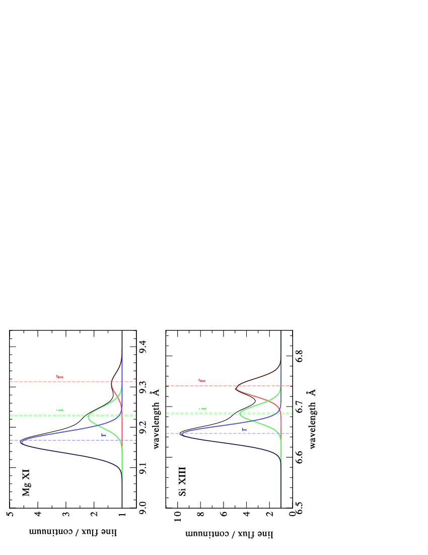
Figure 10: Shows the best-fit input model spectra for two He-like $fir$ line triads (Mg xi& Si xiii) prior to folding through the $MEG\pm 1$ instrumental response functions (ARF & RMF). The input spectra are normalized by their respective continuum. The contributions of each line to the total (black line) line emission is indicated: r-line (blue), i-line (green), and f-line (red). This demonstrates that the high energy resolution capabilities of the HETGS provides a clear distinction of each line’s contribution to the overall emission, and allows us to extract individual $fir$ line characteristics.

For OB stars the $f/i$ ratio provides information on the radial distance from the star to the He-like ion line formation region (Kahn et al. 2001; Waldron & Cassinelli 2001). Even though the He-like $fir$ lines often overlap as demonstrated in Figure 10, line fitting procedures have been successful in extracting the individual fluxes for each of the three $fir$ lines. From our studies of these He-like line formation regions, we have been finding that for most OB stars, the high ion stages are formed with $R_{fir}$ close to the star, which could indicate the presence of magnetically confined regions on the surface (Waldron & Cassinelli 2001).

It is important to point out that since the $f/i$ ratio is sensitive to the assumed photospheric flux model, there is a model dependent uncertainty in the derived $R_{fir}$(e.g., see discussion by Miller et al. 2002). This is particularly relevant for the $R_{fir}$derived from the Ar xvii, S xv, and Si xiii He-like $f/i$ ratios which are sensitive to the unmeasurable flux short-ward of 912 Å. However, since this $f/i$ diagnostic has shown an overall consistent pattern in the radial locations of the He-like X-ray emission lines for several O-stars, we believe that this diagnostic is currently the most viable procedure for estimating the radial locations of the He-like X-ray emission lines, with the understanding that the results are sensitive to the assumed photospheric flux model.

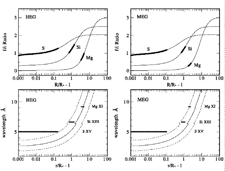
Figure 11: Top - The Cyg OB2 No. 8a HEG and MEG He-like $f/i$ ratio dependence on radius. The observed range of the $f/i$ ratios and their associated radial ranges are indicated by the broad darkened line sectors. Bottom - The corresponding X-ray continuum optical depth unity (solid line) wavelength dependence on radius (assuming the mass loss rate given in Table 2) and the observed range in radii associated with each He-like $f/i$ ratio. In all plots the Ar xvii radial range is not shown since it is below 1.001. The dashed lines correspond to a factor of 2 increase (larger radii) and a factor of 2 decrease (smaller radii) in mass loss rate.

Following the procedure outlined by Waldron & Cassinelli (2001) we have determined the radial positions of the He-like ions of Mg xi, Si xiii, S xv, and Ar xvii. The MEG and HEG $f/i$ ratios and derived radial positions, $R_{fir}$, are given in Table 3. The $f/i$ ratio dependence on radius is shown in Figure 11 where the MEG and HEG observed ranges in $f/i$ and their corresponding radial ranges are indicated by darken curved sectors. Also shown is our standard X-ray continuum optical depth unity plot as a function of radius which shows that the $R_{fir}$ do appear consistent with other OB stellar results, i.e., the observed He-like X-ray emission is predominantly emerging from its associated ‘effective’ X-ray photosphere as first suggested by Waldron & Cassinelli (2001). The calculations of these X-ray continuum optical depth unity radii are discussed in the Appendix. As evident in Figure 11, although the mapping of $R_{fir}$ to the X-ray optical depth unity radii is not exactly one-to-one, the overall mapping does appear to follow the wavelength dependence of the optical depth unity radii reasonably well. One notable exception is that the S xv $R_{fir}$ is significantly smaller than expected. This could imply that the associated high temperatures required to produce this emission are only produced deep in the wind ($<1.1$ stellar radii) and, hence, are actually located at a depth where the X-ray optical depth is slightly $>2$. As seen in other O-stars, we also see that the higher ion stages are progressively closer to the stellar surface and, in particular, Ar xvii, is essentially on the surface (not shown in Figure 11). Figure 11 also shows the wavelength dependencies of the X-ray continuum optical depth unity radii for a mass loss rate 2 times smaller and 2 times larger than the value given in Table 1. The best match between $R_{fir}$ and X-ray optical depth unity radii appears to be associated with a mass loss rate that is $\sim 2$ times smaller. In a recent study, Hanson (2003) suggests that the Cyg OB2 association may be $\sim 35\%$ closer than originally though which would imply a reduction in the radio determined mass loss rate (given in Table 1) by a factor of $\sim 2$.

3.3 Temperature Diagnostics of the X-ray Line Emitting Plasma

Of particular interest regarding OB stars is the temperature of the X-ray emitting plasma. There can be several causes of this X-ray emission, ranging from shocks embedded in winds, bow shock structures either around clumps in winds or around unseen companion stars, or magnetic structures near the base of the wind. For example, determining the relationship between $EM$ and $T$ could provide clues on the X-ray formation process. Here we discuss two line ratio diagnostics techniques to derive X-ray emitting plasma temperatures.

Miller et al. (2002) were the first to apply the H-like to He-like line ratio temperature diagnostic to an early-type star, the late O-star $\delta\$Ori. In general, one might expect problems using this diagnostic for X-rays embedded in a dense wind of an OB star since a small change in position could produce significantly different wind attenuations. However, it is becoming increasingly clear that each X-ray emission line appears to be arising from its associated X-ray continuum optical depth unity position. Hence, when taking line ratios, the attenuation factors are roughly equal and cancel. Normally, the He line used in the $H/He$ line ratio is the sum of all $fir$ lines. However, to avoid the uncertainties associated with the formation of the $f$ and $i$ lines as discussed earlier, we only use the He-like $r$ line in our calculation of the $H/He$ line ratio. We have used the APED data to determine the dependence of the $H/He$ ratio on temperature. Table 4 lists the available H-like to He-like line ratios and their derived X-ray temperatures, $T_{H/HE}$. Notice that both the MEG and HEG derived temperatures are in very good agreement. Since we expect that the two lines associated with each $H/He$ ratio are probably formed in different wind locations, our interpretation of this temperature diagnostic is that it represents the average X-ray temperature between these two locations and, in fact, all of these $T_{H/HE}$ are found to lie within the temperature range specified by their respective H and He line $T_{L}$ values. All of these temperatures along with their associated $R_{fir}$ support earlier claims that, in general, the X-ray temperatures associated with the majority of the observed X-ray emission in OB stellar winds are increasing inward toward the stellar surface.

Another line ratio technique used extensively in solar studies is the He-like $G$-ratio [$G=(f+i)/r$]. Waldron & Cassinelli (2001) were the first to apply this technique to an early-type star, the O-star $\zeta\$Ori, where they found good agreement with $T_{L}$. The observed ISM corrected $G$-ratios for our He-like lines are given in Table 3, and the associated temperatures, $T_{fir}$, are determined by comparing our observed $G$-ratios with $G$-ratios calculated from the APED data. Except for the HEG Mg xi $G$-ratio, there appears to be significant problems with this method as compared with $T_{L}$ and $T_{H/He}$. One possible explanation is that the $r$ line flux may be reduced by strong resonance line scattering which results in a higher $G$-ratio and a smaller temperature (Porquet & Dubau 2000). However, there are relatively large discrepancies in $G$-ratio values quoted throughout the literature. For example, the $G$-ratio temperature relation used in the analysis by Waldron & Cassinelli (2001) is found to be significantly different than those quoted by Porquet & Dubau (2000). As these line ratio discrepancies are resolved, the usefulness of this technique for OB stars needs to be explored in greater detail.

3.4 The Emission Measure Distribution

The range of temperatures in the X-ray forming regions tells us about the nature of the shocks involved. Cohen, Cassinelli, & MacFarlane (1997) found that for the near main sequence star $\tau\$Sco, $EM(T)\propto T^{-2}$. Such a power law result is also found for bow shock models of clump generated X-rays from hydrodynamical theory (Moeckel, Cho & Cassinelli 2002). In the Moeckel et al. bow shock model, it was found that a wide range of ionization conditions could be present both because there can be very hot matter right at the peak of the bow and a whole range of cooler material produced at the oblique shock region of the bow. The detection of Ar xvii line emission, for example, indicates that there is a hotter source of gas in Cyg OB2 No. 8a than in other O-stars we have studied, such as $\zeta\$Pup. Moeckel et al. (2002) showed that the emission measure versus $T$ distribution behind a bow shock is a power law where $EM(T)\propto T^{-4/3}$. The modeling of $\tau\$Sco by Howk et al. (2000) indicated that the wind is strongly influenced by bow shocks. Miller (2002) found a rough power law dependence for $\delta\$Ori with a slope of $-2/3$ and it was argued that there could be a wind collision with a companion star. However, based on the $EM$ values listed in Table 2, there is no clear indication of any temperature dependence and, in fact, one could argue that all line $EM$ values are essentially the same.

3.5 Spectral Fit to the HETG/MEG Spectrum of Cyg No. 8a

In general, fitting the overall HETG spectra of OB stars is a difficult task due to the large range in temperatures, the distribution of X-ray sources, the widely varying degree of stellar wind absorption throughout the wind, the extreme line broadening, and the quenching of the He-like $f$ line. For the case of Cyg OB2 No. 8a, since there is no observed soft X-ray emission due to the large degree of ISM extinction, a model with fewer X-ray source temperatures can be used. Hence, our goal here is to find the simplest model capable of reproducing the overall spectral characteristics observed in the MEG spectrum of Cyg OB2 No. 8a. In addition, this model fit provides us with the total observed X-ray flux in the HETGS energy band width which can be used for comparisons with other observed broad-band X-ray results. We use the ROSAT (Waldron et al. 1998) and ASCA (Kitamoto & Mukai 1996) derived fitting parameters as starting points for establishing temperature and column density estimates. The X-ray emission lines and continuum are calculated using the MEKAL emissivity model (Mewe, Gronenschild, & van den Oord 1985). In addition, to account for the large line broadening and peculiar He-like $fir$ line behavior, the emissivity model had to be modified by considering: 1) all emission lines are assumed to be Gaussian in shape and include a pseudo “turbulent velocity” component to mimic the line broadening (which is reasonable considering that all lines are generally symmetric), and; 2) artificially large X-ray densities are included to suppress the He-like forbidden line emission since the current model has no provisions for modeling the effects of an ambient UV radiation field. The model fits are then obtained by folding the spectral model through the HETGS instrumental response functions (RMF & ARF). The free parameters are the temperatures, wind column densities, and emission measures. The fixed parameters are the ISM column density given in Table 1, a turbulent velocity of 1150 km s^-1, and for the low and high temperature components, the emissivity densities are respectively $3.2\times 10^{13}$ and $1.0\times 10^{13}$ cm^-3. Note, these densities have no physical meaning with regards to the X-ray emitting plasma since they are only used to simulate the correct $f/i$ ratios which are controlled by the stellar UV/EUV radiation field.

We find that a two-temperature, two-wind column density model can provide an adequate overall fit to the MEG spectrum. The resultant temperatures are $3.98\pm 1.67$ and $13.88\pm 1.80$ MK. Their respective wind column densities are $(1.22\pm 0.60)\times 10^{22}$ and $(1.41\pm 0.45)\times 10^{22}$ cm^-2, and their respective intrinsic emission measures are $(3.65\pm 2.41)\times 10^{57}$ and $(1.06\pm 0.24)\times 10^{57}$ cm^-3. The reduced $\chi^{2}$ is 1.29 ($\chi^{2}/DOF$ = 605/470). Comparing these emission measures with the ISM corrected line emission measures at similar temperatures (see Table 2) indicate that these emission measures are approximately 17 and 4 times larger, and the difference is related to the fact that these model derived emission measures represent their intrinsic values (i.e., the $EM_{X}$ in Table 2 have not been corrected for wind absorption). These two temperatures and wind column densities are consistent with the ROSAT and ASCA derived parameters, as well as the observed log $L_{x}/L_{bol}$ of $\sim-6.75$. Although the ROSAT and ASCA fits only required one column density, we found that two wind column densities were required in order to fit the relative strengths of the Mg xii line with respect to the Mg xi and Si xiii lines. The majority of the Mg xi emission is primarily associated with the 3.98 MK component whereas, the majority of the Mg xii and Si xiii line emissions are associated with the 13.88 MK component. Furthermore, these best fit column densities can be used to estimate the location of the two temperature components assuming a spherically symmetric wind (see Waldron et al. 1998). The resultant radius for the 3.98 MK component is $6.44\pm 2.97$ $R_{*}$, and for the 13.88 MK component, the radius is $4.79\pm 1.38$ $R_{*}$. Although the associated errors in these radial positions indicate that these locations are essentially indistinguishable, these model best-fit radial locations do suggest that the hotter component is located slightly deeper in the wind than the cooler component which is consistent with our $fir$ analysis (see Sec. 3.2). In addition, the cool component location is found to fall within the combined MEG and HEG Mg xi $R_{fir}$ range of 2.7 to 6.1 $R_{*}$(see Table 3), and is also consistent with the single component model fit to ROSAT data which predicted an X-ray location of $\sim 4.7$ $R_{*}$ (Waldron et al. 1998). The hot component location is found to be larger than the combined MEG and HEG Si xiii $R_{fir}$ range of 1.7 to 2.4 $R_{*}$. The most likely explanation of this discrepancy is the simplicity of assuming a two-component fit model. For example, by considering a model with a distribution of X-ray temperatures around the current hot component temperature, significantly more emission over a broader spectral energy range would be produced. This excess emission would have to be balanced by an increase in the absorbing wind column density, which in turn would predict a smaller radial location range for this distribution of temperatures. In principle this same argument should also be applicable to the cooler component. However, since most of this soft X-ray emission is masked by the large ISM absorption, and this observed soft emission has very weak lines with essential no continuum, it is understandable why a single temperature component provides a reasonable fit to the softer spectral region.

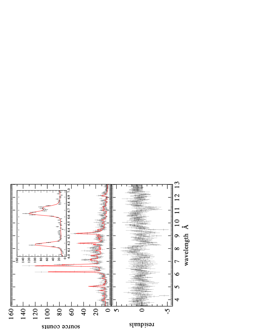
Figure 12: Comparison of the best-fit model spectrum (red line) to the MEG $\pm 1^{st}$ order spectrum for Cyg OB2 No. 8a. The spectrum only covers the wavelength region of the strongest lines. The corresponding residuals of the fit are shown in the bottom panel. The inset highlights the wavelength region of the two strongest lines, Si xiv and Si xiii. The bin size is 0.02 Å.

The comparison of our model fit with the observed spectrum is shown in Figure 12 which only covers the wavelength region of the strongest lines. This shows that the line strengths, broadness, and $f/i$ ratios are in very good agreement. The only real discrepancy is in the region between 7 and 8 Å where the model has a problem in fitting these weaker lines. The Chandra observed log $L_{x}/L_{bol}$ is found to be $\sim-6.75$ which is essentially identical to the value determined when last observed in 1993 (within $\sim$ 20 %). Waldron et al. (1998) studied the long term X-ray variability of these Cyg OB2 stars and noticed that, of the four, the observed X-ray emission from Cyg OB2 No. 8a had remained essentially constant for $\sim 15$ years. We can now suggest that Cyg OB2 No. 8a X-ray emission has now remained constant for the last 24 years. In addition, since the $L_{x}/L_{bol}$ ratio is consistent with the general O-star behavior, we can argue that the X-ray emission processes in Cyg OB2 No. 8a are probably no different than those occurring in isolated O-stars. In particular, Chlebowski (1989) found that the $L_{x}/L_{bol}$ ratio for close binary stars have significantly larger values than the observed $L_{x}/L_{bol}$ value for Cyg OB2 No. 8a.

3.6 Analysis of the Cyg OB2 No. 9 MEG Spectrum

As summarized by Waldron et al. (1998), Cyg OB2 No. 9 is by far one of the most interesting variable stellar radio sources where essentially every time a radio observation is obtained it displays a different structure. For example, it has displayed both thermal and non-thermal characteristics at different epochs. However, even when it does appear in a thermal state, its radio emission is still different, which, assuming free-free emission, indicates a highly variable mass loss rate. On the other hand, with regards to X-ray emission, Cyg OB2 No. 9 is similar to Cyg OB2 No. 8a in that the X-ray emission has remained relatively stable for $\sim 15$ years. In addition, Cyg OB2 No. 9 is also the weakest of the four in terms of X-ray emission and the strongest radio emitter, whereas, Cyg OB2 No. 8a is the strongest X-ray source and the weakest radio source.

Although Cyg OB2 No. 9 is the weakest of the four main stellar X-ray sources in Cyg OB2, it is the closest of the remaining three to the aim point (Cyg OB2 No. 8a), resulting in the second best dispersed spectrum observed. However, the HETG spectrum of Cyg OB2 No. 9 is weak, so detailed analyses like those for Cyg OB2 No. 8a are not possible. Also, the bigger instrumental line spread function makes the emission lines of Cyg OB2 No. 9 more difficult to measure. Nevertheless by using an RMF-based analysis to study these weak emission lines, reasonable reconstructions of line shapes can be obtained. The MEG Si xiii and Si xiv lines are strong enough to extract information on line profile parameters and line fluxes, and reasonable line flux estimates can also be extracted for the Mg xi ($r$ line only) and Mg xii lines. The following flux values have units of ergs cm^-2 s^-1. For Si xiv we find a flux = $0.17\pm 0.03\times 10^{-13}$, V_S = $-100\pm 270$ km s^-1, and a $HWHM<940$ km s^-1. For Si xiii we find a total $fir$ flux$=0.48\pm 0.1\times 10^{-13}$, V_S = $-700\pm 250$ km s^-1, and a $HWHM=620\pm 430$ km s^-1. The individual $fir$ line fluxes in units of $10^{-13}$ are respectively $0.12\pm 0.02$, $0.19\pm 0.03$, and $0.16\pm 0.3$, which yield an $f/i$ ratio of $0.60\pm 0.16$. Correspondingly, the Mg xi $r$ line flux = $0.11\pm 0.02\times 10^{-13}$, and the Mg xii flux = $0.08\pm 0.02\times 10^{-13}$.

From this limited amount of information, we find three interesting results. First, the H-like to He-like line ratios for Mg and Si (see Table 4) provide temperatures that are in very good agreement with the $T_{H/He}$ derived for Cyg OB2 No. 8a. Second, the Si xiii $f/i$ ratio suggests a radial location range between 1.4 to 1.9 stellar radii. As discussed above, Cyg OB2 No. 9 had been observed twice when it had a thermal radio spectrum. The associated mass loss rate estimates from these two times are $12.7\times 10^{-6}$ $M_{\odot}\,$yr^-1 (1983) and $40.0\times 10^{-6}$ $M_{\odot}\,$yr^-1 (1993). Using the 1983 mass loss rate value for determining the X-ray continuum optical depth unity radius for Si xiii  it is found to be $\sim 1.5$ stellar radii. The 1993 value predicts an X-ray continuum optical depth unity radii of $\sim 4$ stellar radii. Since the 1983 value provides a consistent radius with the $f/i$ radius we suggest that the 1983 determined mass loss rate is a better estimate of the mass loss rate for Cyg OB2 No. 9 at the time of our observations. Third, the fit to the Si xiii lines suggests a rather large blue-shift of $\sim-700$ km s^-1. If correct the implications are very interesting, for we know from the $f/i$ ratio that the radial location of Si xiii is between 1.4 to 1.9 stellar radii. These radii correspond to a wind velocity range of 915 to 1200 km s^-1 (using the standard velocity law with a $\beta=0.8$; Groenewegen, Lamers, & Pauldrach 1989). By assuming a saw-tooth wind shock structure as proposed by Lucy & White (1980), this wind velocity range implies a shock velocity range of 215 to 510 km s^-1 and a corresponding shock temperature range of only 0.6 to 3.6 MK, well below the expected temperature needed for formation of Si xiii ($\sim 11$ MK). We also see a similar situation from the Si xiv line and S xvi lines observed in Cyg OB2 No. 8a (see Table 2 and discussion in Sec. 3.1.4). Thus it is difficult to understand these observations in the context of this relatively simple shock model.

The line-spread functions of the other two stars (Cyg OB2 Nos. 5 & 12) are too large to be useful for extracting line shape information and $fir$ analyses which are the focus of this paper. However, their MEG flux spectra are included in Figure 4 which allows one to extract reasonable line flux estimates for the various observed emission lines and provides a comparison of the energy flux spectra of all four stars.

4 Conclusions: Are the X-ray Properties of Cluster Stars Similar to Those of Normal OB Stars?

There are several reasons why the Cyg OB2 region is of special interest. The strongest X-ray source in this region, Cyg OB2 No. 8a, is the second example of a very luminous early O-star and it is one of the very few that Chandra will be able to observe within a reasonable exposure time. Since we are observing a cluster, our one observation provided high resolution spectra of three early O-stars and one B supergiant. These objects could be of special interest because Cyg OB2 might be a young globular cluster. Thus it might be like the X-ray emitting regions observed at lower spectral resolution in other galaxies.

The Cyg OB2 stars are in a relatively tight cluster that has been called a young globular cluster (Knödlseder 2000; Hanson 2003). Hence, it is possible, maybe even likely that there is a contribution to the X-ray flux from all of the stars from wind-wind or wind-star collisions. For example, Bonnell & Bate (2002) found that star formation simulations indicate that massive stars are generally in binary systems which can be relatively wide. Thus while it is likely that $>1/2$ of all OB stars are in binary systems, these could be too widely separated for a predominance of X-rays to be arising from wind-wind collisions. Now if Cyg OB2 No. 8a were to have its X-rays forming from such a collision, then we would see evidence for this in our wavelength versus radius plots. That is, instead of having the radii of line formation located near X-ray optical depth unity, these radii would be much larger, comparable to that of the separation of early-type stars. A hint of such a departure was seen in our study of $\delta\$Ori (Miller et al. 2002), where Si xiii was found to be formed well beyond the X-ray optical depth unity radius. However, for Cyg OB2 No. 8a, since the lines do seem to be formed near X-ray optical depth unity, we do not see a need for postulating anything other than this star being similar to other early-type single stars.

All previous X-ray observations (Einstein, ROSAT, & ASCA) of the brightest Cyg OB2 Association OB stars indicate that these stars show clear evidence that the X-ray emission is significantly hotter than most other OB stars. This is also evident from our Chandra observations where we clearly see Ar xvii and other higher energy ions. From this feature along with the fact that these stars are very massive, many have suggested that these stars are precursors to Wolf-Rayet star formation (e.g., Schaller et al. 1992). Unfortunately, due to the very large ISM extinction for the Cyg OB2 stars, it is very hard to distinguish whether the ISM or wind is the dominant absorbing component for the soft X-ray emission as also noted by Waldron et al. (1998). Based on our two component fit to the Cyg OB2 No. 8a MEG spectrum, we find the wind column densities required to fit the spectrum need to be larger than the ISM column density, suggesting that the wind column density is dominant. However, if these are precursors to WR stars, then why do they have similar standard O-star behavior (e.g., comparable $L_{x}/L_{bol}$  and consistency with X-ray optical depth unity)? Ignace, Oskinova, & Brown (2003) point out that X-ray optical depth unity radii are expected to be in a range of a 100 to 1000 stellar radii for WR stars. One main difference between an O supergiant and a WR star is the stellar radius, and as discussed in Section 3.1, the wind column density scale factor is inversely proportional to the stellar radius. For example, assuming that the mass loss rate and wind speed remains the same and the stellar radius of Cyg OB2 No. 8a is reduced by a factor of 3 (from 30 to 10), we find that the location of X-ray optical depth unity for 15 Å changes from $\sim$ 10 to 50 stellar radii. Furthermore, we know that WR star mass loss rates are typically larger than those of the Cyg OB2 stars which would raise this X-ray optical depth unity radius up to several hundred radii, consistent with WR results.

Although these high X-ray temperatures inferred from our Chandra observation of the Cyg OB2 stars are unusual for O supergiants, they are not overly unusual with regards to all O-stars. For example, the Chandra HETGS observations of the main sequence O5 star, $\theta^{1}$ Ori C, shows evidence for even higher temperatures and is believed to be related to magnetic activity (Schulz et al. 2003). In addition, recent XMM-Newton observations of the late O supergiant $\zeta\$Ori (Mewe, private communication) shows evidence for X-ray emission from Ar xvii which was not seen in the HETGS observations of this star (Waldron & Cassinelli 2001). This is interesting since it may be indicating the presence of a variable high X-ray energy component, possibility associated with surface activity. A ROSAT time series observation of $\zeta\$Ori also indicated the possibility that some sort of ‘flare-like’ event was observed (Berghöfer & Schmitt 1994).

To summarize with regards to our detailed analysis of Cyg OB2 No. 8a, we do not see evidence for the strong wind absorption like that seen in WR stars. We also do not see any strong evidence supporting wind-wind interactions as evident from our $fir$ analysis and the derived $L_{x}/L_{bol}$. Thus we suggest at this point to treat this star as if it is a single O-star X-ray source. Using the single star approach we have come to these interesting conclusions.

a) Two methods were used to derive the radius of X-ray formation, the $f/i$ ratio of He-like ions, and a fitting of the entire spectrum with a two component model with temperatures and column densities for each source as adjustable parameters. Both methods are found to predict that the overall radial range of the Mg xi and Si xiii line formation region is 1.7 to 6.1 stellar radii.

b) Although this radial range is far below the range expected for X-rays from WR stars, this does not rule out the possibility that this star is a proto-WR star.

c) X-rays are forming deep in the wind, as was the case for $\zeta\$Pup and $\zeta\$Ori  and essentially all of the Chandra observed OB stars as shown in the temperature versus radius figure of Cassinelli, Waldron, & Miller (2003). This demonstrates that the simple idea that the X-rays arise from wind shocks of about $1/2$ the local wind speed is not correct. The cause of the hot gas near the stellar surface thus remains a puzzle.

d) Because the Cyg OB2 No 8a and $\zeta\$Pup are similar early O-stars with strong winds, we had expected that Cyg OB2 No. 8a would be more like $\zeta\$Pup in showing skewed and blue-shifted line profiles, but that is not the case. Thus $\zeta\$Pup still appears to be unique among O-stars. However, it also means that there is still a problem in understanding of how OB stars can have symmetric X-ray line profiles. There are several explanations: 1) the winds are so porous owing to fragmentation (e.g., Feldmeier et al. 2003) that one can see farther into the wind, even to the far side of the wind where red-shifting of line occurs; 2) the X-rays are arising from outflowing and in-falling clumps (Howk et al. 2000), but their model should only be valid for stars with very weak winds that allow for stalling and inflow; 3) Ignace & Gayley (2002) suggest that resonance line scattering may reduce the degree of line asymmetry but their use of a Sobolev analysis and its dependence on a smooth velocity gradient seems to be a questionable treatment of an X-ray shock region, and; 4) the X-rays are forming in extended magnetic loops, as had originally been envisioned by Underhill (1980) and we see both hot up flows and down flows in magnetic tubes.

e) We were able to get X-ray information regarding four O-stars with one observation that had a carefully planned satellite orientation. Although we were only able to get the most detailed information from the primary source, Cyg OB2 No. 8a, we demonstrated that we were also able to get some useful emission line information from one other source, Cyg OB2 No. 9, and find some reasonable line flux estimates for the two weakest sources (Cyg OB2 Nos. 5 & 12).

Because the OB stars considered here are in a tight stellar cluster, we have had to consider whether the X-rays were dominated by collisions that produce bow shock structures or by processes involving enhance magnetic confinement of hot plasma. The arguments that we had to consider should be of interest to X-ray astronomers studying galaxies and star burst regions, since they are surely looking at clusters of OB stars somewhat analogous to Cyg OB2. In our analysis we have developed criteria for deciding on the nature of the X-ray emission. In the case of Cyg OB2 No. 8a, we found no evidence that its X-ray emission is dominated by processes other than those occurring in isolated OB stars.

WLW was supported by NASA grant GO2-3028C and acknowledges partial support from NASA grant GO2-3027A. JPC and NAM were supported by NASA grant GO2-3028. NAM and JCR acknowledge support from the UW-Eau Claire Office of Research and Sponsored Programs. We wish to thank Shantih Spanton for some initial discussions of the data.

Appendix A Calculation of X-ray Continuum Optical Depth Unity

Analyses of the He-like ion $f/i$ line ratios in OB stars suggest that the derived $fir$-inferred radii are highly correlated with their respective X-ray continuum optical depth unity radii (i.e., the radial wind location where the X-ray continuum optical depth, $\tau_{\lambda}$ = 1, for a given wavelength). In general, the stellar wind X-ray continuum optical depth for a given wavelength, $\lambda$, measured outward from radius $r$ is defined as

$$\tau_{\lambda}(r)=\int_{r}^{\infty}\sigma_{\lambda}(r^{\prime})n_{H}(r^{\prime})dr^{\prime}$$ (A1)

where $\sigma_{\lambda}(r)$ is the radial and wavelength dependent wind absorption cross section (cm²), and $n_{H}$ is the hydrogen number density (cm^-3) defined in terms of the wind mass density as $n_{H}(r)=\rho(r)/\mu_{H}m_{H}$ (where $m_{H}$ is the atomic weight of hydrogen and $\mu_{H}$ is the mean atomic weight). Although we follow the basic procedure for determining $\sigma_{\lambda}(r)$ as discussed by Waldron (1984), several modifications have been incorporated. In particular, we have updated the photoionization cross sections (including all K-shell cross sections from all ion stages), the collisional and recombination rates (including dielectronic recombination), and all other relevant atomic data (e.g., elemental abundances) that are available in the most recent version of the Raymond & Smith (1979) emissivity code as summarized by Raymond (1988). In addition, the calculation of $\sigma_{\lambda}(r)$ now includes the contributions from 13 elements (H, He, C, N, O, Ne, Mg, Si, S, Ar, Ca, Fe, Ni) and all their stages of ionization.

To obtain an analytic relationship between radius and $\tau_{\lambda}$, two basic assumptions are required. First, it is necessary to simplify the integration in eq. (A1). This is accomplished by assuming that $\sigma_{\lambda}(r)$ can be represented as a density weighted average cross section throughout the wind which is only dependent on the wavelength and independent of the radial position. This density weighted cross section is defined as

$$\sigma_{avg}(\lambda)~{}=~{}\frac{\tau_{\lambda}(\hbox{$R_{*}$})}{N_{W}(\hbox{$R_{*}$})}$$ (A2)

where $\tau_{\lambda}(\hbox{$R_{*}$})$ and $N_{W}(\hbox{$R_{*}$})$ are respectively the total X-ray continuum optical depth and wind column density (cm^-2) as measured from the stellar surface. A representative energy dependent distribution of $\sigma_{avg}(\lambda)$ for the Cyg OB2 O- stars is shown in Waldron et al. (1998). Hence, $\tau_{\lambda}$ can be approximated as

$$\tau_{\lambda}(r)~{}\approx~{}\sigma_{avg}(\lambda)N_{W}(r)~{}=~{}\sigma_{avg}(\lambda)\int_{r}^{\infty}n_{H}(r^{\prime})dr^{\prime}$$ (A3)

where $N_{W}(r)$ represents the wind column density measure outward from the radial position $r$. The error introduced by using the approximate $\tau_{\lambda}$ (eq. A3) as opposed to the actual $\tau_{\lambda}$ (eq. A1) is found to be only a few percent. The second assumption requires specification of the wind geometry and wind velocity law. We adopt a spherically symmetric wind with a wind speed that is determined by the standard $\beta$ velocity law [i.e., $v(r)=\hbox{$v_{\infty}$}(1-\hbox{$R_{*}$}/r)^{\beta}$]. Although this velocity law allows us to obtain a simple analytic expression, it produces a singularity in the wind density at the stellar surface. In the actual calculations used to determine $\sigma_{avg}(\lambda)$ and produce the plots shown in Figure 11, the velocity law is modified by adding a small but finite constant velocity term ($V_{\circ}$) to the standard velocity law, and $N_{W}$ has to be determined numerically. The addition of this constant term places an upper limit to the wind density at $R_{*}$, and the value of $V_{\circ}$ is typically chosen to be equal to approximately one-half of the photospheric sound speed. We realize that for the special case of $\beta=1$, an analytic expression is still obtainable with the addition of $V_{\circ}$, but here we will adopt the more appropriate value of $\beta=0.8$ (Groenewegen et al. 1989). With these assumptions, the value of $N_{W}(r)$ is given by (for $\beta~{}\neq~{}1$)

$$N_{W}(r)~{}=~{}\int_{r}^{\infty}n_{H}(r^{\prime})dr^{\prime}~{}=~{}{\frac{N_{O}}{1-\beta}}[1~{}-~{}w(r)^{1/(\beta-1)}]$$ (A4)

where

$$N_{O}=\frac{{\hbox{$\dot{M}$}}}{4\pi\mu_{H}m_{H}\hbox{$v_{\infty}$}\hbox{$R_{*}$}}~{}~{}~{}{\rm cm}^{-2}$$ (A5)

and $w(r)=v(r)/\hbox{$v_{\infty}$}$. Although our expression for $N_{W}(r)$ given by eq. (A4) is valid for essentially the whole wind structure, it will begin to overestimate $N_{W}$ when $v(r)$ becomes comparable to $V_{O}$ which occurs at radii below $\sim 1.01\hbox{$R_{*}$}$. Below this radius limit the overestimate in $N_{W}$ is initially a few percent, reaching a maximum of $\sim 25\%$ at $R_{*}$. However, the details in this region are immaterial to our discussion concerning the location of X- ray optical depth unity since any depth indicating a location $<1.01\hbox{$R_{*}$}$ can be interpreted as occurring essentially on the stellar surface. For additional details, and the case for $\beta=1$ see Waldron et al. (1998).

Since our goal is to find the relationship between radial position and wavelength for a given value of $\tau_{\lambda}$ (e.g.,$\tau_{\lambda}$), we proceed by first finding an expression for $w(r)$. By combining the results of eqs. (A3) and (A4) we have

$$w(r)=\left[1-{\frac{(1-\beta)\tau_{\lambda}(r)}{\sigma_{avg}(\lambda)N_{\circ}}}\right]^{\beta/(1-\beta)}$$ (A6)

Using the adopted velocity law to obtain the relation between $r$ and $w$, our desired relationship between radius and wavelength for a given $\tau_{\lambda}$ is given by

$$r~{}=~{}\hbox{$R_{*}$}~{}\left(1~{}-\left[1~{}-~{}{\frac{(1-\beta)\tau_{\lambda}}{\sigma_{avg}(\lambda)N_{\circ}}}\right]^{1/(\beta-1)}\right)^{-1}$$ (A7)

Table 1: Adopted Stellar Parameters

	Cyg OB2 No. 9	Cyg OB2 No. 8a	Cyg OB2 No. 5	Cyg OB2 No. 12
Spectral Type	O5f	O5.5 I(f)	O6f+O7f	B8 Ia
$T_{eff}$ (K)	44700	38500	39800	11200
log $L_{bol}$(ergs/s)	40.19	39.77	40.01	39.79
$M$ ($M_{\odot}$)	160	90.5	118	71
$R$ ($R_{\odot}$)	34	27.9	34	338
$v_{\infty}$(km s-1)	2200	2650	2200	1400
$d$ (kpc)	1.82	1.82	1.82	1.82
log $N_{ISM}$(cm${}^{-2})$)	22.06	21.92	22.02	22.23
$v\sin i$(km s-1)	145	95	180	75
$\dot{M}$($M_{\odot}\,$yr-1)	$12.7\times 10^{-6}$	$13.5\times 10^{-6}$	$34.5\times 10^{-6}$	$38.5\times 10^{-6}$

Table 2: X-ray Emission Line Properties for Cyg OB2 No. 8a

Ion	$\lambda_{\circ}$	line flux$/10^{-13}$	V${}_{S}~{}~{}~{}$	$HWHM$	$EM_{x}$	$T_{L}$	$\chi^{2}/DOF$
	Å	erg cm-2 s-1	km s-1	km s-1	$10^{56}$ cm-3	(MK)
Medium Energy Grating
Ne x	12.132	$0.27\pm 0.04$	$0\pm 450$	$651\pm 468$	$1.36\pm 0.50$	$6.82\pm 2.09$	$37.3/46$
Mg xi($fir$)	9.169	$0.64\pm 0.07$	$-191\pm 380$	$998\pm 182$	$2.13\pm 0.68$	$6.71\pm 10.70$	$41.0/42$
Mg xii	8.419	$0.44\pm 0.04$	$-550\pm 314$	$1025\pm 421$	$1.66\pm 0.49$	$11.45\pm 3.51$	$16.2/19$
Si xiii($fir$)	6.648	$2.20\pm 0.16$	$-87\pm 151$	$884\pm 96$	$2.90\pm 0.88$	$11.03\pm 3.09$	$52.1/40$
Si xiv	6.180	$1.08\pm 0.07$	$-36\pm 216$	$1096\pm 316$	$2.56\pm 0.70$	$18.85\pm 6.26$	$17.7/14$
S xv($fir$)	5.039	$1.37\pm 0.27$	$-195\pm 640$	$<830$	$2.23\pm 1.02$	$16.18\pm 4.96$	$28.3/24$
S xvi	4.727	$0.36\pm 0.08$	$245\pm 307$	$986\pm 380$	$1.42\pm 0.55$	$29.32\pm 10.49$	$10.8/10$
Ar xvii($fir$)	3.949	$0.30\pm 0.10$	$-100\pm 250$	$<150$	$1.56\pm 1.14$	$23.74\pm 7.89$	$24.6/22$
High Energy Grating
Ne x	12.132	$0.15\pm 0.05$	$-300\pm 300$	$<1400$	$0.76\pm 0.44$	$6.82\pm 2.09$	$22.2/46$
Mg xi($fir$)	9.169	$0.91\pm 0.16$	$-146\pm 610$	$910\pm 389$	$3.64\pm 1.35$	$6.71\pm 1.70$	$34.5/42$
Mg xii	8.419	$0.59\pm 0.07$	$-432\pm 283$	$1019\pm 320$	$2.24\pm 0.73$	$11.45\pm 3.51$	$26.4/19$
Si xiii($fir$)	6.648	$2.45\pm 0.28$	$-133\pm 479$	$1017\pm 256$	$2.57\pm 0.89$	$11.03\pm 3.09$	$44.5/40$
Si xiv	6.180	$1.11\pm 0.11$	$50\pm 255$	$956\pm 285$	$2.64\pm 0.80$	$18.85\pm 6.26$	$15.9/14$
S xv($fir$)	5.039	$1.86\pm 0.41$	$-832\pm 368$	$533\pm 348$	$2.15\pm 1.04$	$16.18\pm 4.96$	$21.0/24$
S xvi	4.727	$0.52\pm 0.12$	$-35\pm 635$	$<2050$	$2.06\pm 0.94$	$29.32\pm 10.49$	$6.2/10$
Ar xvii($fir$)	3.949	$0.56\pm 0.20$	$-736\pm 258$	$<650$	$3.74\pm 2.06$	$23.74\pm 7.89$	$21.1/22$

Table 3: He-like ion $fir$ Line Properties for Cyg OB2 No. 8a

Ion	$r$ flux	$i$ flux	$f$ flux	G-ratio	$f/i$ ratio	$T_{fir}$	Rfir
						(MK)	$R_{*}$
Medium Energy Grating
Mg xi	$0.45\pm 0.04$	$0.15\pm 0.02$	$0.05\pm 0.01$	$0.48\pm 0.07$	$0.35\pm 0.08$	$>11$	$3.13\pm 0.39$
Si xiii	$1.17\pm 0.07$	$0.46\pm 0.04$	$0.57\pm 0.05$	$0.87\pm 0.10$	$1.20\pm 0.17$	$<5$	$1.96\pm 0.24$
S xv	$0.60\pm 0.10$	$0.41\pm 0.09$	$0.35\pm 0.08$	$1.26\pm 0.44$	$0.85\pm 0.33$	$<5$	$<1.11$
Ar xvii	$0.12\pm 0.05$	$0.18\pm 0.06$	$<0.03$	$1.57\pm 1.04$	$<0.16$	$<25$	$\sim 1.00$
High Energy Grating
Mg xi	$0.52\pm 0.07$	$0.22\pm 0.05$	$0.17\pm 0.04$	$0.76\pm 0.16$	$0.80\pm 0.21$	$5.04\pm 2.71$	$5.13\pm 0.93$
Si xiii	$1.04\pm 0.11$	$0.61\pm 0.08$	$0.80\pm 0.09$	$1.34\pm 0.23$	$1.25\pm 0.24$	$<3$	$2.06\pm 0.37$
S xv	$0.58\pm 0.13$	$0.67\pm 0.14$	$0.61\pm 0.14$	$2.20\pm 0.87$	$0.92\pm 0.35$	$<4$	$<1.18$
Ar xvii	$0.28\pm 0.09$	$0.20\pm 0.07$	$0.08\pm 0.05$	$1.00\pm 0.68$	$0.42\pm 0.37$	$<100$	$\sim 1.00$

Table 4: H-like to He-like Line Ratio Temperatures for Cyg OB2 Nos. 8a and 9

Ions	HETGS/MEG		HETGS/HEG
	Line Ratio	$T_{H/He}$ (MK)	Line Ratio	$T_{H/He}$ (MK)
Cyg No. 8a
Mg xii/ Mg xi(r)	$1.23\pm 0.23$	$8.46\pm 0.52$	$1.40\pm 0.36$	$8.78\pm 0.77$
Si xiv/ Si xiii(r)	$1.01\pm 0.13$	$12.96\pm 0.58$	$1.17\pm 0.23$	$13.61\pm 0.99$
S xvi/ S xv(r)	$0.60\pm 0.24$	$16.50\pm 2.21$	$0.91\pm 0.42$	$18.90\pm 3.32$
Cyg No. 9
Mg xii/ Mg xi(r)	$0.94\pm 0.39$	$7.70\pm 1.02$	—	—
Si xiv/ Si xiii(r)	$1.18\pm 0.42$	$13.60\pm 1.74$	—	—

Figure 2: Observed HEG and MEG $\pm 1^{st}$ order count spectra for Cyg OB2 No. 8a. The most likely line identifications are indicated. The bin size is 0.01 Å.

Figure 3: Observed MEG $\pm 1^{st}$ order count spectrum for Cyg OB2 No. 9. The most likely line identifications are indicated. The bin size is 0.01 Å.

Figure 4: Comparison of the combined MEG $\pm 1^{st}$ order flux spectra for all four stars (Cyg OB2 Nos. 8a, 5, 9, & 12). The rest wavelengths of the H-like and He-like lines are labeled. The off-axis degradation in the flux spectra of Cyg OB2 Nos. 5, 9, & 12 is clearly visible below 6 Å. The bin size is 0.02 Å.

Figure 6: Shows comparisons of the Cyg OB2 No. 8a H-like best-fit line model spectra (solid-line) with their corresponding observed $MEG\pm 1$ count spectra and their associated residuals. The horizontal axis is expressed as the velocity shift relative to the rest wavelength of the line. The horizontal dashed-line in the best-fit plot represents the predicted model counts for the continuum. The vertical dashed-lines in the residual plots represent the best-fit line centroid shift velocities ($V_{S}$). In order to obtain reliable flux measurements of the line and continuum emissions for Ne x, the input model spectrum included the weaker Fe xvii($\sim 12.26$ Å) located at $\sim 3200$ km s^-1. The bin size is 0.01 Å.

Figure 7: Same as Figure 6 except for comparisons with the $HEG\pm 1$ count spectra.

Figure 8: Shows comparisons of the Cyg OB2 No. 8a He-like best-fit line model spectra (solid- line) with their corresponding observed $MEG\pm 1$ count spectra and their associated residuals. The vertical dashed-lines indicated the rest wavelengths of the $fir$ lines. Note, although the $i$ line is actually a doublet, each input model spectrum assumes only one line. The bin size is 0.01 Å.

Figure 9: Same as Figure 8 except for comparisons with the $HEG\pm 1$ count spectra.

References

- (1) Abbott, D. C., Bieging, J. H., & Churchwell, E. 1981, ApJ, 250, 645
- (2) Abbott, D. C., Telesco, C. M., & Wolff, S. C. 1984, ApJ, 279, 225
- (3) Berghöfer, T. W., & Schmitt, J. H. M. M. 1994, A&A., 290, 435
- (4) Berghöfer, T. W., Schmitt, J. H. M. M., Danner, R., & Cassinelli, J. P. 1997,A&A., 322, 167
- (5) Bieging, J. H., Abbott, D. C., & Churchwell, E. B. 1989, ApJ, 340, 518
- (6) Blumenthal, G. R., Drake, G. W. F., & Tucker, W. H. 1972, ApJ, 172, 205
- (7) Bonnell, I. A., & Bate, M. R. 2002, MNRAS, 336, 659
- (8) Bonnell, I. A., Vine, S. G., & Bate, M. R. 2004, MNRAS, 349, 735
- (9) Cassinelli, J. P., & Olson, G. L. 1979, ApJ, 229, 403
- (10) Cassinelli, J. P., Waldron, W. L., Sanders, W., Harnden, F., Rosner, R., & Vaiana, G. 1981, ApJ 250,677
- (11) Cassinelli, J. P., Miller, N. A., Waldron, W. L., MacFarlane, J. J., & Cohen, D. H. 2001, ApJ 554, L55
- (12) Cassinelli, J. P., & Swank, J. H. 1983, ApJ, 271, 681
- (13) Cassinelli, J. P., Waldron, W. L., & Miller, N. A. 2003, NASA MSFC Symp., 4 Years of Chandra Observations: A Tribute to Riccardo Giacconi, Sept. 16-18
- (14) Chandra X-Ray Center (CXC) 2002, Chandra Proposers’ Observatory Guide, Rev. 5.0, 2002, TD 403.00.005 (Cambridge, MA: CXC)
- (15) Chlebowski, T. 1989, ApJ, 342, 1091
- (16) Cooper, G. 1994, Ph.D. Thesis, University of Delaware
- (17) Cohen, D., Cassinelli, J. P., & MacFarlane J. J. 1997, ApJ, 487, 687
- (18) Corcoran, M. F. et al. 1993, ApJ, 412, 792
- (19) Feldmeier, A. 1995, A&A, 299, 523
- (20) Feldmeier, A., Shlosman, I., & Hamann, W. -R. 2002, ApJ, 566, 392
- (21) Feldmeier, A., Oskinova, L., & Hamann, W. -R. 2003, A&A, 403, 217
- (22) Groenewegen, M. A. T., Lamers, H. J. G. L. M., & Pauldrach, A. W. A. 1989, A&A, 221, 78
- (23) Hanson, M. M. 2003, ApJ, 597, 957
- (24) Harnden, F. R.et al. 1979, ApJ, 234, L51
- (25) Herrero, A., Puls, J., & Najarro, F. 2002, A&A, 296, 949
- (26) Howk, J. C., Cassinelli, J. P., Bjorkman, J. E., & Lamers, H. J. G. L. M. 2000, ApJ, 534, 348
- (27) Ignace, R., & Gayley, K. 2002, ApJ, 568, 594
- (28) Ignace, R., Oskinova, L. M., & Brown, J. C. 2003, A&A, 408, 353
- (29) Kahn, S. M., Leutenegger, M. A., Cottam, J., Rauw, G., Vreux, J.-M., den Boggende, A. J. F., Mewe, R., & Güdel, M. 2001, A&A, 365, L312
- (30) Kitamoto, S. & Mukai, K. 1996, PASJ, 48, 813
- (31) Knödlseder, J. 2000, A&A, 360, 539
- (32) Kramer, R. H., Cohen, D. H., & Owocki, S. P. 2003, ApJ, 592, 532.
- (33) Lamers, H. J. G. L. M. & Cassinelli, J. P. 1999, “Introduction to Stellar Winds“, Univ. Cambridge Press
- (34) Lucy, L. B. & White, R. L. 1980, ApJ, 241, 300
- (35) MacFarlane, J. J., Cassinelli, J. P., Welsh, B. Y., Vedder, P. W., Vallerga, J. V., & Waldron, W. L. 1991, ApJ, 380, 564
- (36) MacFarlane, J. J., Waldron, W. L., Corcoran, M. F., Wolff, M. J., Wang, P., & Cassinelli, J. P. 1993, ApJ, 419, 813
- (37) Mewe, R., Gronenschild, E. H. B. M., & van den Oord, G. H. J. 1985, A&AS, 62, 197
- (38) Miller, N. A., Cassinelli, J. P., Waldron, W. L., MacFarlane, J. J., & Cohen, D. H. 2002, ApJ, 577, 951
- (39) Miller, N. A., 2002, Ph.D. Thesis, University of Wisconsin.
- (40) Moeckel, N., Cho, J., & Cassinelli, J. P. 2002, BAAS, 200, 7418
- (41) Porquet, D., & Dubau, J. 2000, A&A, 143, 495
- (42) Owocki, S. P., Castor, J. I., & Rybicki, G. B. 1988, ApJ, 335, 914
- (43) Owocki, S. P., & Cohen, D. H. 2001 ApJ, 559, 1108
- (44) Raymond, J. C. 1988, Hot Thin Plasmas in Astrophysics, ed., R. Pallavicini, (Dordrecht: Kluwer), p. 3
- (45) Raymond, J. C., & Smith, B. W. 1979, ApJS, 35, 419
- (46) Schaller, G., Shaerer, D., Meynet, G., & Maeder, A. 1992, A&AS, 96, 269
- (47) Schulz, N. S., Canizares, C. R., Huenemoerder, D., & Tibbets, K. 2003, ApJ, 595, 365
- (48) Shull, J. M., & Van Steenberg, M. E. 1985, ApJ, 294, 599.
- (49) Smith, R. K., & Brickhouse, N. S. 2000, Rev. Mexicana Astron. Astrofis. Ser. Conf., 9, 134
- (50) Snow, T., & Morton D. 1977, ApJS, 33, 269
- (51) Underhill, A. B. 1980, ApJ, 239, 414
- (52) Waldron, W. L. 1984, ApJ, 282, 256
- (53) Waldron, W. L., & Cassinelli, J. P. 2001 ApJ, 548, L45
- (54) Waldron, W. L., & Cassinelli, J. P. 2002, ASP Conf. Ser., The High Energy Universe at Sharp Focus: Chandra Science, Vol. 262, eds., E. M. Schlegel & S. Dil Vrtilek, (San Francisco), p. 69
- (55) Waldron, W. L., Corcoran, M. F., Drake, S. A., & Smale, A. P. 1998,ApJS, 118, 217