Effects of differential and uniform rotation on nonlinear electromotive force in a turbulent flow

Abstract

An effect of the differential rotation on the nonlinear electromotive force in MHD turbulence is found. It includes a nonhelical $\alpha$ effect which is caused by a differential rotation, and it is independent of a hydrodynamic helicity. There is no quenching of this effect contrary to the quenching of the usual $\alpha$ effect caused by a hydrodynamic helicity. The nonhelical $\alpha$ effect vanishes when the rotation is constant on the cylinders which are parallel to the rotation axis. The mean differential rotation creates also the shear-current effect which changes its sign with the nonlinear growth of the mean magnetic field. However, there is no quenching of this effect. These phenomena determine the nonlinear evolution of the mean magnetic field. An effect of a uniform rotation on the nonlinear electromotive force is also studied. A nonlinear theory of the ${\bf\Omega}{\bf\times}\bar{\bf J}$ effect is developed, and the quenching of the hydrodynamic part of the usual $\alpha$ effect which is caused by a uniform rotation and inhomogeneity of turbulence, is found. Other contributions of a uniform rotation to the nonlinear electromotive force are also determined. All these effects are studied using the spectral $\tau$ approximation (the third-order closure procedure). An axisymmetric mean-field dynamo in the spherical and cylindrical geometries is considered. The nonlinear saturation mechanism based on the magnetic helicity evolution is discussed. It is shown that this universal mechanism is nearly independent of the form of the flux of magnetic helicity, and it requires only a nonzero flux of magnetic helicity. Astrophysical applications of these effects are discussed.

I INTRODUCTION

Generation of magnetic fields by a turbulent flow of conducting fluid is a fundamental problem which has a large number of applications in solar physics, astrophysics, geophysics, planetary physics and in laboratory studies (see, e.g., M78 ; P79 ; KR80 ; ZRS83 ; RSS88 ; S89 ; RS92 ; B2000 ; RH04 , and references therein). In recent time the problem of nonlinear mean-field magnetic dynamo is a subject of active discussions (see, e.g., BB96 ; K99 ; GD94 ; GD96 ; KRR95 ; S96 ; CH96 ; KR99 ; FB99 ; RK2000 ; RK2001 ; KMRS2000 ; KMRS02 ; BB02 ; BS04 , and references therein). The conventional approach to the nonlinear dynamo is based on comparison of the three effects participating in dynamo action, namely the $\alpha$ effect (caused by helical motions of a turbulent fluid), the large-scale differential (nonuniform) rotation $\delta\Omega$ and the turbulent magnetic diffusivity $\eta_{{}_{T}}$. The mean magnetic field is generated due to a combined effect of the differential rotation and the $\alpha$ effect. These effects have been considered as independent phenomena. In particular, the electromotive force has been determined independently of the differential rotation.

On the other hand, the differential rotation can be regarded as large-scale motions with a mean velocity shear imposed on the small-scale turbulent fluid flow. An interaction of the mean differential rotation with the small-scale turbulent motions can cause a generation of a mean magnetic field even in a nonhelical, homogeneous and incompressible turbulent fluid flow. This mechanism of mean-field dynamo is associated with a shear-current effect which is determined by the $\bar{\bf W}{\bf\times}\bar{\bf J}$ term in the electromotive force, where $\bar{\bf W}$ is the mean vorticity caused by the mean velocity shear and $\bar{\bf J}$ is the mean electric current (see RK03 ). A nonlinear theory of a shear-current effect in a nonrotating homogeneous and nonhelical turbulence with an imposed mean velocity shear in a plane geometry was developed in RK04 . It was shown that during the nonlinear growth of the mean magnetic field, the shear-current effect changes its sign, but there is no quenching of this effect contrary to the quenching of the usual $\alpha$ effect, the nonlinear turbulent magnetic diffusion, etc.

In this study we investigated the effects of differential and uniform rotation on nonlinear electromotive force. The main conclusion of this study is that the nonlinear electromotive force cannot be determined independently of the mean differential rotation. We found a nonhelical $\alpha$ effect which is caused by a differential rotation and is independent of a hydrodynamic helicity. There is no quenching of this effect contrary to the quenching of the usual $\alpha$ effect caused by a hydrodynamic helicity. The mean differential rotation of fluid can decrease the total $\alpha$ effect due to the nonhelical $\alpha$ effect. Two kinds of the $\alpha$ effect (helical and nonhelical) have opposite signs. Therefore, the total $\alpha$ effect should always change its sign during the nonlinear growth of the mean magnetic field because there is a quenching of the usual (helical) $\alpha$ effect. This can saturate the growth of the mean magnetic field.

The mean differential rotation creates also the shear-current effect. We found that the mean differential rotation increases the growth rate of the large-scale dynamo instability at a weak mean magnetic field due to the shear-current effect, and causes a saturation of the growth of the mean magnetic field at a stronger field. Note that the applications of the obtained results to the solar convective zone shows that the nonlinear shear-current effect becomes dominant at least at the base of the convective zone. We found that the nonlinear function $\sigma_{0}(\bar{B})$ defining the shear-current effect is the same for a turbulence with a mean differential rotation in cylindrical and spherical geometries for an axisymmetric mean field dynamo problem and for a nonrotating turbulence with an imposed linear mean velocity shear in a plane geometry. The latter case was investigated in RK04 .

We also studied an effect of a uniform rotation on the nonlinear electromotive force. In particular, we developed a nonlinear theory of the ${\bf\Omega}{\bf\times}\bar{\bf J}$ effect and we determined the nonlinear quenching of the hydrodynamic part of the $\alpha$ effect which is caused by both, a uniform rotation and inhomogeneity of turbulence. Other nonlinear coefficients defining the nonlinear electromotive force are also determined as a function of a uniform rotation. In this study we considered a uniform rotation with a small rotation rate in comparison with the correlation time of the fluid turbulent velocity field. We studied all the above effects using the spectral $\tau$ approximation (the third-order closure procedure).

This paper is organized as follows. In Section II we formulated the assumptions and the method of the derivation of the nonlinear electromotive force in a turbulence with a uniform and nonuniform rotations. In Section III we considered axisymmetric mean-field dynamo equations and determined the coefficients defining the electromotive force for a rotating turbulence. In Section III we also discussed in details the effects of differential and uniform rotation on nonlinear coefficient defining the electromotive force. In Section IV we analyzed the nonlinear saturation of the mean magnetic field and discussed the astrophysical applications of the obtained results. In Appendix A we derived the nonlinear electromotive force in a turbulence with uniform and nonuniform rotations.

II THE METHOD OF DERIVATIONS

In a framework of the mean-field approach the evolution of the mean magnetic field $\bar{\bf B}$ is determined by equation

$${\partial\bar{\bf B}\over\partial t}=\mbox{\boldmath$\nabla$}\times(\bar{\bf U}\times\bar{\bf B}+\mbox{\boldmath$\cal E$}-\eta\mbox{\boldmath$\nabla$}\times\bar{\bf B})\;$$ (1)

(see, e.g., M78 ; P79 ; KR80 ; ZRS83 ; RSS88 ; S89 ), where $\bar{\bf U}$ is a mean velocity (the differential rotation), $\eta$ is the magnetic diffusion due to the electrical conductivity of fluid. The general form of the electromotive force $\mbox{\boldmath$\cal E$}=\langle{\bf u}\times{\bf b}\rangle$ in an anisotropic turbulence is given by

$${\cal E}_{i} = \alpha_{ij}\bar{B}_{j}+({\bf V}^{\rm eff}{\bf\times}\bar{\bf B})_{i}-\eta_{ij}(\mbox{\boldmath$\nabla$}{\bf\times}\bar{\bf B})_{j}$$ (2)

$$-[\mbox{\boldmath$\delta$}{\bf\times}(\mbox{\boldmath$\nabla$}{\bf\times}\bar{\bf B})]_{i}-\kappa_{ijk}(\partial\hat{B})_{jk}\;$$

(see R80 ; RKR03 ), where $(\partial\hat{B})_{ij}=(1/2)(\nabla_{i}\bar{B}_{j}+\nabla_{j}\bar{B}_{i}),$ ${\bf u}$ and ${\bf b}$ are fluctuations of the velocity and magnetic field, respectively, angular brackets denote averaging over an ensemble of turbulent fluctuations, the tensors $\alpha_{ij}$ and $\eta_{ij}$ describe the $\alpha$-effect and the turbulent magnetic diffusion, respectively, ${\bf V}^{\rm eff}$ is the effective diamagnetic (or paramagnetic) velocity, $\kappa_{ijk}$ and $\delta$ describe an evolution of the mean magnetic field in an anisotropic turbulence. Nonlinearities in the mean-field dynamo imply dependencies of the coefficients $(\alpha_{ij},\eta_{ij},{\bf V}^{\rm eff},$ etc.) defining the electromotive force on the mean magnetic field.

The method of the derivation of equation for the nonlinear electromotive force in a rotating turbulence is similar to that used in RK04 for a nonrotating turbulence with an imposed mean velocity shear. We consider the case of large hydrodynamic and magnetic Reynolds numbers. The momentum equation and the induction equation for the turbulent fields in a frame rotating with an angular velocity ${\bf\Omega}$ are given by

$${\partial{\bf u}(t,{\bf x})\over\partial t} = -{\mbox{\boldmath$\nabla$}p_{\rm tot}\over\rho_{0}}+{1\over\mu\rho_{0}}[({\bf b}\cdot\mbox{\boldmath$\nabla$})\bar{\bf B}+(\bar{\bf B}\cdot\mbox{\boldmath$\nabla$}){\bf b}]$$ (3)

$$+2{\bf u}{\bf\times}{\bf\Omega}-(\bar{\bf U}\cdot\mbox{\boldmath$\nabla$}){\bf u}-({\bf u}\cdot\mbox{\boldmath$\nabla$})\bar{\bf U}$$

$$+{\bf u}^{N}+{\bf F}\,,$$

$${\partial{\bf b}(t,{\bf x})\over\partial t} = (\bar{\bf B}\cdot\mbox{\boldmath$\nabla$}){\bf u}-({\bf u}\cdot\mbox{\boldmath$\nabla$})\bar{\bf B}-(\bar{\bf U}\cdot\mbox{\boldmath$\nabla$}){\bf b}$$ (4)

$$+({\bf b}\cdot\mbox{\boldmath$\nabla$})\bar{\bf U}+{\bf b}^{N}\,,$$

where $\mbox{\boldmath$\nabla$}\cdot{\bf u}=0$, $\,\rho_{0}$ is the fluid density, $\mu$ is the magnetic permeability of the fluid, $\rho_{0}{\bf F}$ is a random external stirring force, ${\bf u}^{N}$ and ${\bf b}^{N}$ are the nonlinear terms which include the molecular dissipative terms, $p_{\rm tot}=p+\mu^{-1}\,(\bar{\bf B}\cdot{\bf b})$ are fluctuations of the total pressure, $p$ are fluctuations of the fluid pressure. Hereafter we omit the magnetic permeability of the fluid, $\mu$, in equations, i.e., we include $\mu^{-1/2}$ in the definition of magnetic field. We study the effect of a mean rotation of the fluid on the nonlinear electromotive force. We split rotation into uniform and differential parts. By means of Eqs. (3)-(4) written in a Fourier space we derive equations for the correlation functions of the velocity field $f_{ij}({\bf k})=\hat{L}(u_{i};u_{j})$, of the magnetic field $h_{ij}({\bf k})=\hat{L}(b_{i};b_{j})$ and for the cross helicity $g_{ij}({\bf k})=\hat{L}(b_{i};u_{j})$, where

$$\hat{L}(a;c)=\int\langle a(t,{\bf k}+{\bf K}/2)c(t,-{\bf k}+{\bf K}/2)\rangle$$

$$\times\exp{(i{\bf K}{\bf\cdot}{\bf R})}\,d{\bf K}\;,$$ (5)

and ${\bf R}$ and ${\bf K}$ correspond to the large scales, and ${\bf r}$ and ${\bf k}$ to the small ones (see, e.g., RS75 ; KR94 ). The equations for these correlation functions are given by Eqs. (40)-(42) in Appendix A. These equations for the second moments contain high moments and a closure problem arises (see, e.g., O70 ; MY75 ; Mc90 ). We apply the spectral $\tau$ approximation or the third-order closure procedure (see, e.g., O70 ; PFL76 ; KRR90 ; KMR96 ; RK2000 ; RK2001 ; KR03 ; BK04 ), which allows to express the deviations of the third moments from the background turbulence in ${\bf k}$ space in terms of the corresponding deviations of the second moments, e.g.,

$$\hat{D}f_{ij}^{N}-\hat{D}f_{ij}^{N(0)} = -(f_{ij}-f_{ij}^{(0)})/\tau(k)\;,$$ (6)

$$\hat{D}h_{ij}^{N}-\hat{D}h_{ij}^{N(0)} = -(h_{ij}-h_{ij}^{(0)})/\tau(k)\;,$$ (7)

$$\hat{D}g_{ij}^{N} = -g_{ij}/\tau(k)\;,$$ (8)

where the tensors $\hat{D}f_{ij}^{N},$ $\,\hat{D}h_{ij}^{N}$ and $\hat{D}g_{ij}^{N}$ are related to the third moments in equations for the second moments $f_{ij},h_{ij}$ and $g_{ij},$ respectively (see Eqs. (40)-(42) in Appendix A). The correlation functions with the superscript ${(0)}$ determine the background turbulence (with a zero mean magnetic field, $\bar{\bf B}=0),$ and $h_{ij}^{(0)}$ is the nonhelical part of the tensor of magnetic fluctuations of the background turbulence, $\tau(k)$ is the characteristic relaxation time of the statistical moments. We applied the $\tau$-approximation only for the nonhelical part $h_{ij}$ of the tensor of magnetic fluctuations. The helical part $h_{ij}^{(H)}$ depends on the magnetic helicity, and it is determined by the dynamic equation which follows from the magnetic helicity conservation arguments KR82 ; ZRS83 (see also GD94 ; KRR95 ; KR99 ; KMRS2000 ; KMRS02 ; BB02 ). In the present paper we consider an intermediate nonlinearity which implies that the mean magnetic field is not enough strong in order to affect the correlation time of turbulent velocity field. We also consider uniform rotation with a small rotation rate in comparison with the correlation time of the fluid turbulent velocity field $(\Omega\,\tau_{0}\ll 1).$ The mean velocity shear due to the differential rotation is considered to be weak $(\delta\Omega\,\tau_{0}\ll 1).$ For the integration in ${\bf k}$-space of the second moments we use the following model of the background turbulence (with zero mean magnetic field, $\bar{\bf B}=0$ and without rotation):

$$f_{ij}^{(0)}({\bf k}) = E(k)\biggl{\{}\langle{\bf u}^{2}\rangle^{(0)}\biggl{[}\delta_{ij}-k_{ij}+{i\over 2k^{2}}(k_{i}\Lambda_{j}^{(v)}$$ (9)

$$-k_{j}\Lambda_{i}^{(v)})\biggr{]}-\frac{1}{2k^{2}}\biggl{[}\varepsilon_{ijn}(2ik_{n}+k_{mn}\nabla_{m})$$

$$-(k_{in}\varepsilon_{jnm}+k_{jn}\varepsilon_{inm})\nabla_{m}\biggr{]}\mu^{v}\biggr{\}}\;,$$

$$h_{ij}^{(0)}({\bf k}) = \langle{\bf b}^{2}\rangle^{(0)}E(k)\biggl{[}\delta_{ij}-k_{ij}+{i\over 2k^{2}}(k_{i}\Lambda_{j}^{(b)}$$ (10)

$$-k_{j}\Lambda_{i}^{(b)})\biggr{]}\;,$$

where $\varepsilon_{ijk}$ is the Levi-Civita tensor, $\delta_{ij}$ is the Kronecker tensor, $k_{ij}=k_{i}k_{j}/k^{2},$ $\,E(k)=-(d\bar{\tau}(k)/dk)/8\pi k^{2},$ $\,\tau(k)=2\tau_{0}\bar{\tau}(k),$ $\,\bar{\tau}(k)=(k/k_{0})^{1-q},$ $\,1<q<3$ is the exponent of the kinetic energy spectrum (e.g., $q=5/3$ for Kolmogorov spectrum), $k_{0}=1/l_{0},$ and $l_{0}$ is the maximum scale of turbulent motions, $\tau_{0}=l_{0}/u_{0}$, $\,u_{0}$ is the characteristic turbulent velocity in the scale $l_{0}$, $\,\Lambda_{i}^{(v)}=\nabla_{i}\langle{\bf u}^{2}\rangle^{(0)}/\langle{\bf u}^{2}\rangle^{(0)},$ $\,\Lambda_{i}^{(b)}=\nabla_{i}\langle{\bf b}^{2}\rangle^{(0)}/\langle{\bf b}^{2}\rangle^{(0)},$ and $\mu^{v}=\langle{\bf u}\cdot(\mbox{\boldmath$\nabla$}{\bf\times}{\bf u})\rangle^{(0)}$ is the hydrodynamic helicity of the background turbulence, $\int f_{ij}^{(0)}({\bf k})\,d{\bf k}=(\langle{\bf u}^{2}\rangle^{(0)}/3)\delta_{ij}$ and $\int h_{ij}^{(0)}({\bf k})\,d{\bf k}=(\langle{\bf b}^{2}\rangle^{(0)}/3)\delta_{ij}.$ Note that $g_{ij}^{(0)}({\bf k})=0.$ Here we neglected a very small magnetic helicity in the background turbulence. However, the magnetic helicity in a turbulence with a nonzero mean magnetic field is not small (see Section III-D). The derived equations allow us to determine the nonlinear electromotive force ${\cal E}_{i}=\varepsilon_{imn}\int g_{nm}({\bf k})\,d{\bf k}$ in a rotating turbulence (see for details, Appendix A).

III THE NONLINEAR ELECTROMOTIVE FORCE IN A ROTATING TURBULENCE FOR AN AXISYMMETRIC DYNAMO

We consider the axisymmetric $\alpha\Omega$-dynamo problem. In cylindrical coordinates $(\rho,\varphi,z)$ the axisymmetric mean magnetic field, $\bar{\bf B}=B(\rho,z)\,{\bf e}_{\varphi}+\mbox{\boldmath$\nabla$}{\bf\times}[A(\rho,z){\bf e}_{\varphi}]$, is determined by the dimensionless equations

$${\partial A\over\partial t} = \biggl{[}\alpha(\bar{\bf B})+W_{\ast}\,\sigma_{1}(\bar{\bf B})\,\nabla_{z}(\delta\Omega)\biggr{]}\,B+\eta_{{}_{A}}(\bar{\bf B})\Delta_{s}A$$ (11)

$$-{1\over\rho}({\bf V}_{A}(\bar{\bf B})\cdot\mbox{\boldmath$\nabla$})(\rho\,A)-W_{\ast}\,\sigma_{0}(\bar{\bf B})\,(\hat{\Omega}B)$$

$$-\Omega_{\ast}\,\delta_{0}^{\Omega}(\bar{\bf B})\,(\mbox{\boldmath$\hat{\omega}$}\cdot\mbox{\boldmath$\nabla$})B\;,$$

$${\partial B\over\partial t} = D\,(\hat{\Omega}A)+\rho\mbox{\boldmath$\nabla$}\cdot\biggl{[}{1\over\rho^{2}}[\eta_{{}_{B}}\mbox{\boldmath$\nabla$}-{\bf V}_{B}(\bar{\bf B})](\rho\,B)\biggr{]}\;,$$

where $\Omega_{\ast}=3\,\Omega\,\tau_{0}/R_{\alpha}=[\Omega/(\delta\Omega)_{\ast}]\,W_{\ast}$ , $\,W_{\ast}=(l_{0}/L)^{2}\,(R_{\omega}/R_{\alpha})$, $\,\mbox{\boldmath$\hat{\omega}$}={\bf\Omega}/\Omega$ and

$$(\hat{\Omega}B) = [\nabla_{z}(\delta\Omega)\nabla_{\rho}-\nabla_{\rho}(\delta\Omega)\nabla_{z}](\rho\,B)\;,$$

$${\bf V}_{A}(\bar{\bf B}) = {\bf V}_{d}(\bar{B})-{\phi_{3}(\bar{B})\over 2}{\bf\Lambda}^{(B)}-{\phi_{2}(\bar{B})\over\rho}{\bf e}_{\rho}\;,$$

$${\bf V}_{B}(\bar{\bf B}) = {\bf V}_{d}(\bar{B})+{\phi_{2}(\bar{B})+\phi_{3}(\bar{B})\over\rho}{\bf e}_{\rho}\;,$$

$${\bf V}_{d}(\bar{B}) = -{\phi_{1}(\bar{B})\over 2}({\bf\Lambda}^{(v)}-\epsilon{\bf\Lambda}^{(b)})\,{L\over L_{{}_{T}}}\;,$$

and $\Delta_{s}=\Delta-1/\rho^{2}$, and $\,{\bf\Lambda}^{(B)}=(\mbox{\boldmath$\nabla$}\bar{\bf B}^{2})/\bar{\bf B}^{2}$. The nonlinear coefficients $\alpha(\bar{\bf B})$, $\,\eta_{{}_{A}}(\bar{B}),$ $\,\eta_{{}_{B}}(\bar{B})$ defining the nonlinear $\alpha$ effect and the nonlinear turbulent magnetic diffusion of the poloidal and toroidal components of the mean magnetic field, are determined by Eqs. (15) and (21) in Section III-A. The nonlinear coefficients $\sigma_{0}(\bar{B})$ defining the shear-current effect and $\sigma_{1}(\bar{B})$ defining the nonhelical $\alpha$ effect, are determined in Section III-B. The coefficient $\delta_{0}^{\Omega}(\bar{B})$ defining the nonlinear ${\bf\Omega}{\bf\times}\bar{\bf J}$ effect, is determined in Section III-C. The quenching functions $\phi_{n}(\bar{B})$ are determined by Eqs. (22) in Section III-A. Note that in the equations for the nonlinear effective drift velocities ${\bf V}_{A}(\bar{\bf B})$ and ${\bf V}_{B}(\bar{\bf B})$ of the poloidal and toroidal components of the mean magnetic field we neglected small contributions $\sim O[(l_{0}/L)^{2}]$ caused by the mean differential rotation.

Equations (11) and (LABEL:L9) are written in the dimensionless form, where length is measured in units of $L$, time in units of $L^{2}/\eta_{{}_{T}}$ and the mean magnetic field $\bar{B}$ is measured in units of the equipartition energy $\bar{B}_{\rm eq}=\sqrt{\rho_{0}}\,u_{0}$, the magnetic potential $A$ is measured in units of $R_{\alpha}\,L\,\bar{B}_{\rm eq}$, the nonlinear $\alpha$ is measured in units of $\alpha_{\ast}$ (the maximum value of the hydrodynamic part of the $\alpha$ effect), the basic scale of the turbulent motions $l$ and turbulent velocity $\sqrt{\langle{\bf u}^{2}\rangle}$ at the scale $l$ are measured in units of their maximum values $l_{0}$ and $u_{0}$, respectively, the dimensionless parameters $\Lambda^{(v)}$ and $\Lambda^{(b)}$ are measured in the units of $L^{-1}_{{}_{T}}$ and $\Lambda^{(B)}$ is measured in the units of $L^{-1}$, the differential rotation $\delta\Omega$ is measured in units of $(\delta\Omega)_{\ast}$, the nonlinear turbulent magnetic diffusion coefficients $\eta_{{}_{A,B}}(\bar{B})$ are measured in the units of $\eta_{{}_{T}}$ and the nonlinear effective drift velocities ${\bf V}_{A,B}(\bar{B})$ are measured in the units of $\eta_{{}_{T}}/L$. We define $R_{\alpha}=L\alpha_{\ast}/\eta_{{}_{T}},$ $\,R_{\omega}=(\delta\Omega)_{\ast}\,L^{2}/\eta_{{}_{T}}$, the characteristic value of the turbulent magnetic diffusivity $\eta_{{}_{T}}=l_{0}u_{0}/3$, the dynamo number $D=R_{\omega}R_{\alpha}$ and ${\rm Rm}=l_{0}u_{0}/\eta$ is the magnetic Reynolds number.

In spherical coordinates $(r,\theta,\varphi)$ the axisymmetric mean magnetic field, $\bar{\bf B}=B(r,\theta)\,{\bf e}_{\varphi}+\mbox{\boldmath$\nabla$}{\bf\times}[A(r,\theta){\bf e}_{\varphi}]$, is determined by the dimensionless equations

$${\partial A\over\partial t} = \biggl{[}\alpha(\bar{\bf B})+W_{\ast}\,\sigma_{1}(\bar{\bf B})\,\nabla_{z}(\delta\Omega)\biggr{]}\,B+\eta_{{}_{A}}(\bar{\bf B})\Delta_{s}A$$ (13)

$$-{1\over r\sin\theta}({\bf V}_{A}(\bar{\bf B})\cdot\mbox{\boldmath$\nabla$})\tilde{A}-W_{\ast}\,\sigma_{0}(\bar{\bf B})\,(\hat{\Omega}B)$$

$$-\Omega_{\ast}\,\delta_{0}^{\Omega}(\bar{\bf B})\,(\mbox{\boldmath$\hat{\omega}$}\cdot\mbox{\boldmath$\nabla$})B\;,$$

$${\partial B\over\partial t} = D\,(\hat{\Omega}A)+r\,\sin\theta\,\mbox{\boldmath$\nabla$}\cdot\biggl{[}{1\over r^{2}\,\sin^{2}\theta}[\eta_{{}_{B}}\mbox{\boldmath$\nabla$}$$ (14)

$$-{\bf V}_{B}(\bar{\bf B})]\tilde{B}\biggr{]}\;,$$

where $\tilde{A}=r\,\sin\theta\,A$, $\,\tilde{B}=r\,\sin\theta\,B$,

$$(\hat{\Omega}B) = [\nabla_{r}(\delta\Omega)\,\nabla_{\theta}-\nabla_{\theta}(\delta\Omega)\,\nabla_{r}]\tilde{B}\;,$$

$$\nabla_{z} = \cos\theta\,\nabla_{r}-\sin\theta\,\nabla_{\theta}\;,$$

$${\bf V}_{A}(\bar{\bf B}) = {\bf V}_{d}(\bar{B})-{\phi_{3}(\bar{B})\over 2}{\bf\Lambda}^{(B)}-{\phi_{2}(\bar{B})\over r}\,({\bf e}_{r}+\cot\theta\,{\bf e}_{\theta}),$$

$${\bf V}_{B}(\bar{\bf B}) = {\bf V}_{d}(\bar{B})+{\phi_{2}(\bar{B})+\phi_{3}(\bar{B})\over r}\,({\bf e}_{r}+\cot\theta\,{\bf e}_{\theta})\;,$$

$\Delta_{s}=\Delta-1/(r\,\sin\theta)^{2}$ and $\nabla_{\theta}=(1/r)\,(\partial/\partial\theta)$. Note that $\rho=r\,\sin\theta$.

III.1 The nonlinear $\alpha$ effect and the nonlinear turbulent magnetic diffusion coefficients of the mean magnetic field

The nonlinear $\alpha$ effect is given by $\alpha(\bar{\bf B})=\alpha^{v}+\alpha^{m},$ where $\alpha^{v}=\chi^{v}\phi^{v}(\bar{B})+\alpha^{\Omega}$ is the hydrodynamic part of the $\alpha$ effect, and $\alpha^{m}=\chi^{c}(\bar{\bf B})\phi^{m}(\bar{B})$ is the magnetic part of the $\alpha$ effect, and the dimensionless parameter $\chi^{v}=-\tau_{0}\,\mu^{v}/3\alpha_{\ast}$ is related to the hydrodynamic helicity $\mu^{v}=\langle{\bf u}\cdot(\mbox{\boldmath$\nabla$}{\bf\times}{\bf u})\rangle^{(0)}$ of the background turbulence, the dimensionless function $\chi^{c}(\bar{\bf B})=(\tau_{0}/3\rho_{0}\alpha_{\ast})\langle{\bf b}\cdot(\mbox{\boldmath$\nabla$}{\bf\times}{\bf b})\rangle$ is related to the current helicity $\langle{\bf b}\cdot(\mbox{\boldmath$\nabla$}{\bf\times}{\bf b})\rangle$. Here $\chi^{v}$ and $\chi^{c}$ are measured in units of $\alpha_{\ast}$, $\,\tau_{0}=l_{0}/u_{0}$ is the correlation time of turbulent velocity field and $\alpha^{\Omega}$ is the contribution to the hydrodynamic part of the $\alpha$ effect caused by a uniform rotation and inhomogeneity of turbulence. Thus,

$$\alpha(\bar{\bf B})=\chi^{v}\phi^{v}(\bar{B})+\alpha^{\Omega}+\chi^{c}(\bar{\bf B})\phi^{m}(\bar{B})\;,$$ (15)

[see Eqs. (67) and (89) in Appendix A], where

$$\alpha^{\Omega} = -{2\over 3}\,{L\,\Omega_{\ast}\over L_{{}_{T}}}\,\mbox{\boldmath$\hat{\omega}$}{\bf\cdot}[\phi^{\Omega}_{1}(\bar{B})\,{\bf\Lambda}^{(v)}+\epsilon\,\phi^{\Omega}_{2}(\bar{B})\,{\bf\Lambda}^{(b)}]\;,$$ (16)

the quenching functions $\phi^{v}(\bar{B})$ and $\phi^{m}(\bar{B})$ are given by

$$\phi^{v}(\bar{B}) = {12\over 7\beta^{2}}\,\biggl{[}1-{\arctan\beta\over\beta}\biggr{]}+{3\over 7}\tilde{L}(\beta)\;,$$ (17)

$$\phi^{m}(\bar{B}) = {3\over\beta^{2}}\,\biggl{[}1-{\arctan\beta\over\beta}\biggr{]}\;$$ (18)

(see RK2000 ), where $\beta=\sqrt{8}\bar{B}$ and $\tilde{L}(y)=1-2y^{2}+2y^{4}\ln(1+y^{-2}).$ Thus $\phi^{v}(\bar{B})=2/\beta^{2}$ and $\phi^{m}(\bar{B})=3/\beta^{2}$ for $\beta\gg 1;$ and $\phi^{v}(\bar{B})=1-(6/5)\beta^{2}$ and $\phi^{m}(\bar{B})=1-(3/5)\beta^{2}$ for $\beta\ll 1.$ The quenching functions $\phi^{\Omega}_{1}(\bar{B})$ and $\phi^{\Omega}_{2}(\bar{B})$ are determined by Eqs. (90) and  (91) in Appendix A. The function $\chi^{c}(\bar{\bf B})$ entering the magnetic part of the $\alpha$ effect is determined by the dynamical equation (29). Note that in Eq. (15) we neglected small contributions $\sim O(\delta\Omega/\Omega)$ caused by the mean differential rotation and inhomogeneity of turbulence [these effects are given by Eqs. (107)-(109) in Appendix A]. For a nonhelical background turbulence the first term, $\chi^{v}\phi^{v}(\bar{B})$, in Eq. (15) vanishes.

The contribution to the nonlinear $\alpha$ effect caused by a uniform rotation for a weak mean magnetic field $\bar{B}\ll\bar{B}_{\rm eq}/4$ is given by

$$\alpha^{\Omega} = -{16\over 15}\,{L\,\Omega_{\ast}\over L_{{}_{T}}}\,\mbox{\boldmath$\hat{\omega}$}{\bf\cdot}\biggl{[}\,{\bf\Lambda}^{(v)}-{\epsilon\over 3}\,{\bf\Lambda}^{(b)}$$ (19)

$$-{180\over 7}\,\biggl{(}{\bf\Lambda}^{(v)}-{3\epsilon\over 5}\,{\bf\Lambda}^{(b)}\biggr{)}\,\bar{B}^{2}\biggr{]}\;,$$

and $\bar{B}\gg\bar{B}_{\rm eq}/4$ it is given by

$$\alpha^{\Omega} = -{1\over 3\beta^{2}}\,{L\,\Omega_{\ast}\over L_{{}_{T}}}\,\mbox{\boldmath$\hat{\omega}$}{\bf\cdot}({\bf\Lambda}^{(v)}+\epsilon\,{\bf\Lambda}^{(b)})$$ (20)

$$-{11\,\Omega_{\ast}\over 3\beta}\,(\mbox{\boldmath$\hat{\omega}$}{\bf\cdot}{\bf\Lambda}^{(B)})\,(1-1.3\epsilon)\;,$$

[see Eqs. (92) and (95) in Appendix A], where the parameter $\epsilon=\langle{\bf b}^{2}\rangle^{(0)}/\langle{\bf u}^{2}\rangle^{(0)}$ is the ratio of the magnetic and kinetic energies in the background turbulence. Asymptotic formula (19) for $\alpha^{\Omega}$ in the limit of a very small mean magnetic field coincides with that obtained in RKR03 for $q=5/3$.

The splitting of the nonlinear $\alpha$ effect into the hydrodynamic, $\alpha^{v}$, and magnetic, $\alpha^{m}$, parts was first suggested in PFL76 . The magnetic part $\alpha^{m}$ includes two types of nonlinearity: the algebraic quenching described by the function $\phi^{m}(\bar{B})$ (see FB99 ; RK2000 ) and the dynamic nonlinearity which is determined by Eq. (29). The algebraic quenching of the $\alpha$-effect is caused by the direct and indirect modification of the electromotive force by the mean magnetic field. The indirect modification of the electromotive force is caused by the effect of the mean magnetic field on the velocity fluctuations and on the magnetic fluctuations, while the direct modification is due to the effect of the mean magnetic field on the cross-helicity (see RK2000 ; RK2001 ).

The nonlinear turbulent magnetic diffusion coefficients of the mean magnetic field are given by

$$\eta_{{}_{A}}(\bar{B}) = \phi_{1}(\bar{B})\;,\quad\eta_{{}_{B}}(\bar{B})=\phi_{1}(\bar{B})+\phi_{3}(\bar{B})\;$$ (21)

(see RK04 ), where the quenching functions $\phi_{k}(\bar{B})$ are given by

$$\phi_{1}(\bar{B}) = A_{1}^{(1)}(4\bar{B})+A_{2}^{(1)}(4\bar{B})\;,$$ (22)

$$\phi_{2}(\bar{B}) = -{1\over 2}(1+\epsilon)A_{2}^{(1)}(4\bar{B})\;,$$

$$\phi_{3}(\bar{B}) = (2-3\epsilon)A_{2}^{(1)}(4\bar{B})-(1-\epsilon){3\over 2\pi}\bar{A}_{2}(16\bar{B}^{2})\;,$$

the functions $\bar{A}_{k}(y)$ and $A_{k}^{(1)}(y)$ are given by Eqs. (61)-(63) in Appendix A. The asymptotic formulas for the functions $\phi_{k}(\bar{B})$ for $\bar{B}\ll\bar{B}_{\rm eq}/4$ are given by $\phi_{1}(\bar{B})=1-(12/5)\,\beta^{2}$, $\,\phi_{2}(\bar{B})=1-(4/5)\,(1+\epsilon)\,\beta^{2}$ and $\phi_{3}(\bar{B})=-(8/5)\,(1-2\epsilon)\,\beta^{2}$. For $\bar{B}\gg\bar{B}_{\rm eq}/4$ they are given by $\phi_{1}(\bar{B})=1/\beta^{2}$, $\,\phi_{2}(\bar{B})=\phi_{3}(\bar{B})=2(1+\epsilon)/3\beta$, where $\beta=\sqrt{8}\bar{B}$. Note that in Eq. (21) we neglected small contributions $\sim O[(l_{0}/L)^{2}]$ caused by the mean differential rotation.

III.2 The nonlinear coefficients $\sigma_{0}(\bar{B})$ and $\sigma_{1}(\bar{B})$ defining the shear-current effect and the nonhelical $\alpha$ effect

The nonlinear coefficient $\sigma_{0}(\bar{B})$ describes the shear-current effect (see RK03 ; RK04 ) and $\sigma_{1}(\bar{B})$ determines the nonhelical $\alpha$ effect. The parameters $\sigma_{0}(\bar{B})$ and $\sigma_{1}(\bar{B})$ are determined by the corresponding contributions from the $\mbox{\boldmath$\delta$}(\bar{\bf B})$ term, the ${\eta}_{ij}(\bar{\bf B})$ term and the ${\kappa}_{ijk}(\bar{\bf B})$ term in the nonlinear electromotive force (2) caused by the mean differential rotation. We found that the nonlinear function $\sigma_{0}(\bar{B})$ defining the shear-current effect is the same for a turbulence with a mean differential rotation in cylindrical and spherical geometries for an axisymmetric mean field dynamo problem and for a nonrotating turbulence with an imposed linear mean velocity shear in a plane geometry. The latter case was studied in RK04 .

To explain the physics of the shear-current effect, we compare the $\alpha$ effect in the $\alpha{\bf\Omega}$ dynamo with the $\delta$ term caused by the shear-current effect (see RK03 ; RK04 ). The $\alpha$ term in the nonlinear electromotive force which is responsible for the generation of the mean magnetic field and caused by a uniform rotation and inhomogeneity of turbulence, reads ${\cal E}^{\alpha}_{i}\equiv\alpha^{v}\bar{B}_{i}\propto-({\bf\Omega}\cdot{\bf\Lambda}^{(v)})\bar{B}_{i}$ (see RKR03 ), where ${\bf\Lambda}^{(v)}$ determines the inhomogeneity of turbulence. The $\delta$ term in the electromotive force caused by the shear-current effect is given by ${\cal E}^{\delta}_{i}\equiv-(\mbox{\boldmath$\delta$}{\bf\times}(\mbox{\boldmath$\nabla$}{\bf\times}\bar{\bf B}))_{i}\propto-(\bar{\bf W}\cdot\mbox{\boldmath$\nabla$})\bar{B}_{i}$ (see RK03 ), where the $\delta$ term is proportional to the mean vorticity $\bar{\bf W}=\mbox{\boldmath$\nabla$}{\bf\times}\bar{\bf U}$ which is caused by the differential rotation.

During the generation of the mean magnetic field in both cases (in the $\alpha{\bf\Omega}$ dynamo and in the shear-current dynamo), the mean electric current along the original mean magnetic field arises. The $\alpha$ effect is related to the hydrodynamic helicity $\propto({\bf\Omega}\cdot{\bf\Lambda}^{(v)})$ in an inhomogeneous turbulence. The deformations of the magnetic field lines are caused by upward and downward rotating turbulent eddies in the $\alpha{\bf\Omega}$ dynamo. Since the turbulence is inhomogeneous (which breaks a symmetry between the upward and downward eddies), their total effect on the mean magnetic field does not vanish and it creates the mean electric current along the original mean magnetic field (see P79 ).

In a turbulent flow with the mean differential rotation, the inhomogeneity of the original mean magnetic field breaks a symmetry between the influence of upward and downward turbulent eddies on the mean magnetic field. The deformations of the magnetic field lines in the shear-current dynamo are caused by upward and downward turbulent eddies which result in the mean electric current along the mean magnetic field and produce the magnetic dynamo (see RK03 ; RK04 ).

Note that the differential rotation is described by the gradient tensor of the mean velocity field $\nabla_{i}\bar{U}_{j}=(\partial\hat{U})_{ij}+\varepsilon_{ijn}(\mbox{\boldmath$\bf\nabla$}{\bf\times}\bar{\bf W})_{n}/2$, where the symmetric part of the gradient tensor $({\partial\hat{U}})_{ij}=(\nabla_{i}\bar{U}_{j}+\nabla_{j}\bar{U}_{i})/2$ is given by

$$(\partial\bar{U})_{ij}={1\over 2}[({\bf e}_{z}{\bf\times}{\bf r})_{i}\nabla_{j}+({\bf e}_{z}{\bf\times}{\bf r})_{j}\nabla_{i}]\,(\delta\Omega)\;,$$ (23)

and the mean vorticity $\bar{\bf W}$ in cylindrical coordinates is given by

$$\bar{\bf W}=-\rho\,({\bf e}_{\rho}\,\nabla_{z}-{\bf e}_{z}\,\nabla_{\rho})\,(\delta\Omega)\;,$$ (24)

and in spherical coordinates the mean vorticity is

$$\bar{\bf W}=r\sin\theta\,({\bf e}_{r}\,\nabla_{\theta}-{\bf e}_{\theta}\,\nabla_{r})\,(\delta\Omega)\;.$$ (25)

The nonlinear coefficients $\sigma_{0}(\bar{B})$ and $\sigma_{1}(\bar{B})$ defining the shear-current effect and the nonhelical $\alpha$ effect are determined by Eqs. (103) and (LABEL:F5) in Appendix A. The nonlinear dependencies of the parameters $\sigma_{0}(\bar{B})$ and $\sigma_{1}(\bar{B})$ are shown in FIG. 1 for different values of the parameter $\epsilon$. The background magnetic fluctuations caused by the small-scale dynamo and described by the parameter $\epsilon$, increase the parameter $\sigma_{0}(\bar{B})$. For a weak mean magnetic field $\bar{B}\ll\bar{B}_{\rm eq}/4$ the parameter $\sigma_{0}(\bar{B})$ is given by $\sigma_{0}(\bar{B})=(4/45)\,(2-q+3\epsilon)$ (see RK04 ), where $q$ is the exponent of the energy spectrum of the background turbulence. The latter equation is in agreement with that obtained in RK03 where the case a weak mean magnetic field and $\epsilon=0$ was considered. In this equation we neglected small contribution $\sim O[(4\bar{B}/\bar{B}_{\rm eq})^{2}]$. The mean magnetic field is generated due to the shear-current effect, when $\sigma_{0}(\bar{B})>$, i.e., when the exponent of the energy spectrum $q<2+3\epsilon$. Note that the parameter $q$ varies in the range $1<q<3$. Therefore, when the level of the background magnetic fluctuations caused by the small-scale dynamo is larger than $1/3$ of the kinetic energy of the velocity fluctuations, the mean magnetic field can be generated due to the shear-current effect for an arbitrary exponent $q$ of the energy spectrum of the velocity fluctuations (see RK04 ).

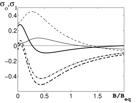
Figure 1: The nonlinear coefficient $\sigma_{0}(\bar{B})$ defining the shear-current effect for $\epsilon=0$ (thin solid) and for $\epsilon=1$ (thin dashed); and the nonlinear coefficient $\sigma_{1}(\bar{B})$ defining the nonhelical $\alpha$ effect for different values of the parameter $\epsilon$: $\,\,\,\epsilon=0$ (thick solid); $\epsilon=17/21$ (thick dashed-dotted); $\epsilon=1$ (thick dashed).

For the Kolmogorov turbulence, i.e., when the exponent of the energy spectrum of the background turbulence $q=5/3$, the parameters $\sigma_{0}(\bar{B})$ and $\sigma_{1}(\bar{B})$ for $\bar{B}\ll\bar{B}_{\rm eq}/4$ are given by $\sigma_{0}(\bar{B})=(4/135)\,(1+9\epsilon)$ and $\sigma_{1}(\bar{B})=(2/135)\,(17-21\epsilon)$. For $\bar{B}\gg\bar{B}_{\rm eq}/4$ they are given by $\sigma_{0}(\bar{B})=-(11/135)\,(1+\epsilon)$ and $\sigma_{1}(\bar{B})=(2/135)\,(1+\epsilon)$. It is seen from these equations and from FIG. 1 that the nonlinear coefficient $\sigma_{0}(\bar{B})$ changes its sign at some value of the mean magnetic field $\bar{B}=\bar{B}_{\ast}$. For instance, $\bar{B}_{\ast}=0.6\bar{B}_{\rm eq}$ for $\epsilon=0$, and $\bar{B}_{\ast}=0.3\bar{B}_{\rm eq}$ for $\epsilon=1$. However, there is no quenching of this effect contrary to the quenching of the nonlinear $\alpha$ effect, the nonlinear turbulent magnetic diffusion, the nonlinear ${\bf\Omega}{\bf\times}\bar{\bf J}$ effect, etc.

The mean differential rotation causes the nonhelical $\alpha$ effect, $W_{\ast}\,\sigma_{1}(\bar{\bf B})\,\nabla_{z}(\delta\Omega)$ [see Eqs. (11) and (13)], which is independent of a hydrodynamic helicity. It follows from the asymptotic formula for $\sigma_{1}(\bar{B})$ at $\bar{B}\gg\bar{B}_{\rm eq}/4$ that there is no quenching of this effect contrary to the quenching of the regular nonlinear $\alpha$ effect (see Section III-A). These two kinds of the $\alpha$ effect have opposite signs. Thus, the total $\alpha$ effect should change its sign during the nonlinear growth of the mean magnetic field. The nonhelical $\alpha$ effect vanishes if the mean rotation is constant on the cylinders which are parallel to the rotation axis. Note that $\sigma_{1}(\bar{B}=0.1\bar{B}_{\rm eq})=0$ for $\epsilon=1$.

The $\delta$ term in the electromotive force which is responsible for the shear-current effect has been also calculated in RS05 ; RKICH05 for a kinematic problem using the second-order correlation approximation (SOCA). However, these studies did not found the dynamo action in nonrotating and nonhelical shear flows. Note that the second order correlation approximation (SOCA) is valid for small hydrodynamic Reynolds numbers. Indeed, even in a highly conductivity limit (large magnetic Reynolds numbers) SOCA can be valid only for small Strouhal numbers, while for large hydrodynamic Reynolds numbers (fully developed turbulence) the Strouhal number is unity. Our recent studies for small hydrodynamic and magnetic Reynolds numbers (using spectral $\tau$ approximation) also did not found the dynamo action in nonrotating and nonhelical shear flows in agreement with RS05 ; RKICH05 .

III.3 The nonlinear coefficient $\delta_{0}^{\Omega}(\bar{B})$ defining the ${\bf\Omega}{\bf\times}\bar{\bf J}$ effect

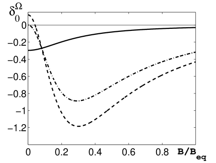
Figure 2: The nonlinear coefficient $\delta_{0}^{\Omega}(\bar{B})$ defining the ${\bf\Omega}{\bf\times}\bar{\bf J}$ effect for different values of the parameter $\epsilon$: $\,\,\,\epsilon=0$ (dashed); $\epsilon=2/7$ (dashed-dotted); $\epsilon=1$ (solid).

The $\delta$ term in the electromotive force which is caused by a uniform rotation, describes the ${\bf\Omega\times\bar{J}}$ effect. This effect in combination with the differential rotation can cause a generation of the mean magnetic field even in a nonhelical turbulent flow (see R69 ; R72 ; MP82 ; R86 and RKR03 ), where $\bar{\bf J}$ is the mean electric current. The nonlinear coefficient $\delta_{0}^{\Omega}(\bar{B})$ defining the ${\bf\Omega}{\bf\times}\bar{\bf J}$ effect is determined by

$$\delta_{0}^{\Omega}(\bar{B}) = -{2\over 3}\biggl{[}\Psi_{4}\{C_{1}+C_{3}\}_{y}-(1-\epsilon)(\Psi_{2}+4\Psi_{3})\{A_{1}$$

$$+A_{2}\}_{y}+(1+\epsilon)(A_{1}^{(2)}(y)+A_{2}^{(2)}(y))\biggr{]}_{y=4\bar{B}}\;,$$

where the functions $\Psi_{k}\{X\}_{y}$ are determined by Eqs. (83) in Appendix A. The parameter $\delta_{0}^{\Omega}(\bar{B})$ is determined by the contributions from the $\mbox{\boldmath$\delta$}(\bar{\bf B})$ term, the ${\eta}_{ij}(\bar{\bf B})$ term and the ${\kappa}_{ijk}(\bar{\bf B})$ term in the nonlinear electromotive force (2) caused by a uniform rotation. The nonlinear coefficient $\delta_{0}^{\Omega}(\bar{B})$ is shown in FIG. 2 for different values of the parameter $\epsilon$. The asymptotic formulas for the coefficient $\delta_{0}^{\Omega}(\bar{B})$ for a weak mean magnetic field $\bar{B}\ll\bar{B}_{\rm eq}/4$ are

$$\delta_{0}^{\Omega}(\bar{B}) = {8\over 135}(2-7\epsilon)\;,$$ (27)

and for $\bar{B}\gg\bar{B}_{\rm eq}/4$ are

$$\delta_{0}^{\Omega}(\bar{B}) = -{1\over 3\beta^{2}}(34+19\epsilon)\;.$$ (28)

Asymptotic formula (27) for a weak mean magnetic field $(\bar{B}\ll\bar{B}_{\rm eq}/4)$ coincide with that obtained in RKR03 for $q=5/3$.

III.4 The dynamical equation for the function $\chi^{c}(\bar{\bf B})$

The function $\chi^{c}(\bar{\bf B})$ entering the magnetic part of the $\alpha$ effect [see Eq. (15)] is determined by the dynamical equation

$${\partial\chi^{c}\over\partial t} = -4\biggl{(}{L\over l_{0}}\biggr{)}^{2}[\mbox{\boldmath$\cal E$}{\bf\cdot}\bar{\bf B}+\mbox{\boldmath$\nabla$}\cdot\mbox{\boldmath$\cal F$}^{(\chi)}]$$ (29)

$$-\mbox{\boldmath$\nabla$}\cdot(\bar{\bf U}\chi^{c})-\chi^{c}/T\;,$$

(see, e.g., KR82 ; KR99 ), where $\mbox{\boldmath$\cal F$}^{(\chi)}$ is the nonadvective flux of the magnetic helicity which serves as an additional nonlinear source in the equation for $\chi^{c}$ (see KMRS2000 ; KMRS02 ), $\,\bar{\bf U}\chi^{c}$ is the advective flux of the magnetic helicity, $\bar{\bf U}$ is the differential rotation, and $T=(1/3)(l_{0}/L)^{2}{\rm Rm}$ is the characteristic time of relaxation of magnetic helicity. Equation (29) was obtained using arguments based on the magnetic helicity conservation law. The function $\chi^{c}$ is proportional to the magnetic helicity, $\chi^{c}=2\chi^{m}/(9\mu\eta_{{}_{T}}\rho_{0})$ (see KR99 ), where $\chi^{m}=\langle{\bf a}\cdot{\bf b}\rangle$ is the magnetic helicity and ${\bf a}$ is the vector potential of small-scale magnetic field. The physical meaning of Eq. (29) is that the total magnetic helicity is a conserved quantity and if the large-scale magnetic helicity grows with mean magnetic field, the evolution of the small-scale helicity should somehow compensate this growth. Compensation mechanisms include dissipation and various kinds of transport (see KMRS2000 ; KMRS02 ).

In order to demonstrate an important role of the nonadvective flux of the magnetic helicity, let us consider a local model in cylindrical coordinates, when the mean magnetic field depend only on the vertical coordinate $z$ and $A^{\prime}\gg A/r$, where $A^{\prime}=\partial A/\partial z$ and $\bar{\bf B}=B{\bf e}_{\varphi}-A^{\prime}{\bf e}_{r}$. Since

$${\partial A\over\partial t}={\cal E}_{\varphi}\;,$$ (30)

$${\partial B\over\partial t}={\cal E}^{\prime}_{r}-DA^{\prime}\;,$$ (31)

we obtain that

$$\mbox{\boldmath$\cal E$}{\bf\cdot}\bar{\bf B}={\cal E}_{\varphi}B-{\cal E}_{r}A^{\prime}=B{\partial A\over\partial t}+{\cal E}_{r}{1\over D}{\partial B\over\partial t}-{1\over 2D}({\cal E}_{r}^{2})^{\prime}\;,$$

(32)

Then in steady state Eqs. (29) and (32) yield

$${\cal E}_{r}^{2}-2D{\cal F}^{(\chi)}_{z}=const\;,$$ (33)

where ${\cal E}_{r}=\eta_{{}_{B}}B^{\prime}$. Here we neglected the last term in Eq. (29) which, e.g., for galactic dynamo is very small. In a steady-state for fields of even parity with respect to the disc plane, we obtain the solution of Eq. (33) for positive $C\,D$

$$\int_{0}^{B}{\eta_{{}_{B}}(\tilde{B})\over\sqrt{|{\cal F}(\tilde{B})}|}\,d\tilde{B}=\sqrt{2|C\,D|}\int_{|z|}^{1}\sqrt{|\chi^{v}(\tilde{z})|}\,d\tilde{z}\;,$$ (34)

where ${\cal F}^{(\chi)}_{z}=C|{\cal F}(B)||\chi^{v}(z)|.$ The crucial point for the dynamo saturation is a nonzero flux of magnetic helicity. It follows from Eq. (34) that this saturation mechanism is nearly independent of the form of the flux of magnetic helicity. In that sense this is a universal mechanism which limits growth of the mean magnetic field. If we assume that $|\mbox{\boldmath$\cal F$}(\bar{B})|\sim\bar{B}^{-2\gamma_{\ast}}$, we obtain that the saturated mean magnetic field is

$$\bar{B}_{\varphi}=|C\,D|^{1\over 2\gamma_{\ast}}\biggl{[}\int_{|z|}^{1}\sqrt{|\chi^{v}(\tilde{z})|}\,d\tilde{z}\biggr{]}^{1\over\gamma_{\ast}}\,\bar{B}_{\rm eq}\;,$$ (35)

where we redefined the constant $C$, we took into account that $\eta_{{}_{B}}(\bar{B})\propto B_{\rm eq}/\bar{B}$ for $\bar{B}\gg\bar{B}_{\rm eq}/4$, and we restored the dimensional factor $\bar{B}_{\rm eq}.$ Note that the nonadvective flux of the magnetic helicity was chosen in KMRS02 in the form $\mbox{\boldmath$\cal F$}^{(\chi)}=C\chi^{v}\phi_{v}(\bar{B})\bar{\bf B}^{2}\eta_{A}^{(z)}(\bar{B})(\mbox{\boldmath$\nabla$}\rho_{0})/\rho_{0}$. This corresponds to $\gamma_{\ast}=1$ in the function $|\mbox{\boldmath$\cal F$}(B)|$. For the specific choice of the profile $|\chi^{v}(z)|=\sin^{2}(\pi z/2)$ we obtain

$$\bar{B}_{\varphi} \approx {4\over 1+\epsilon}\sqrt{|C\,D|}\,\bar{B}_{\rm eq}\cos\,\biggl{(}{{\pi z}\over 2}\biggr{)}\;,$$ (36)

$$\bar{B}_{r} \approx -{1+\epsilon\over 4|R_{\omega}|}\bar{B}_{\rm eq}\tan\,\biggl{(}{{\pi z}\over 2}\biggr{)}\;,$$ (37)

where we have now restored the dimensional factor $\bar{B}_{\rm eq}.$ The boundary conditions for $\bar{B}_{\varphi}$ are $\bar{B}_{\varphi}(z=1)=0$, $\,B_{\varphi}^{\prime}(z=0)=0$, and for $B_{r}$ are $B_{r}(z=1)=0$, $\,B_{r}^{\prime}(z=0)=0.$ Note, however, that this asymptotic analysis performed for $\bar{B}\gg\bar{B}_{\rm eq}/4$ is not valid in the vicinity of the point $z=1$ because $\bar{B}(z=1)=0$.

III.5 The dynamo waves

In order to elucidate the new effects caused by the differential rotation, let us consider first a kinematic problem in a spherical geometry. Following P55 we study dynamo action in a thin convective shell, average the linearized equations (13) and (14) for $A$ and $B$ over the depth of the convective shell. Then we neglect the curvature of the convective shell and replace it by a flat slab. These equations are obviously oversimplified. However, they can be used to reproduce basic qualitative features of solar and stellar activity (see, e.g., KKMR03 ). We are interested in dynamo waves propagating from middle solar latitudes towards the equator. We seek for a solution of the obtained equations in the form of the growing waves, $A,B\propto\exp(\gamma\,t)\exp[i(\omega\,t-{\bf K}\cdot{\bf R})]$, where the growth rate of the dynamo waves with the frequency

$$\omega=-\alpha_{l}\,\sqrt{{D\,|S_{K}|\over 2}}\,{{\rm sgn}(S_{K})\over\sqrt{\sigma_{l}+\sqrt{\sigma_{l}^{2}+\alpha_{l}^{2}}}}$$ (38)

is given by

$$\gamma=\sqrt{{D\,|S_{K}|\over 2}\,\biggl{[}\sigma_{l}+\sqrt{\sigma_{l}^{2}+\alpha_{l}^{2}}\biggr{]}}-K^{2}\;.$$ (39)

The frequency and the growth rate of the dynamo waves are written in a dimensionless form. Here

$$\alpha_{l} = \alpha+W_{\ast}\,\sigma_{1}\,S_{z}\;,$$

$$\sigma_{l} = W_{\ast}\,\sigma_{0}\,S_{K}+\Omega_{\ast}\,\delta_{0}^{\Omega}\,K_{z}\;,$$

$$S_{K} = K_{\theta}\,\nabla_{r}(\delta\Omega)-K_{r}\,\nabla_{\theta}(\delta\Omega)\;,$$

$$S_{z} = \cos\theta\,\nabla_{r}(\delta\Omega)-\sin\theta\,\nabla_{\theta}(\delta\Omega)\;,$$

$$K_{z} = \cos\theta\,K_{r}-\sin\theta\,K_{\theta}\;.$$

The total $\alpha$ effect, $\alpha_{l}$, is a sum of the usual $\alpha$ effect (caused by helical motions) and a nonhelical contribution, $W_{\ast}\,\sigma_{1}\,S_{z}$, due to the effect of the the mean differential rotation on the small-scale turbulence. The parameter $\sigma_{l}$ describes both, the shear-current effect determined by $W_{\ast}\,\sigma_{0}\,S_{K}$ term, and the ${\bf\Omega}{\bf\times}\bar{\bf J}$ effect determined by $\Omega_{\ast}\,\delta_{0}^{\Omega}\,K_{z}$ term. Even in nonhelical turbulent motions, the mean magnetic field is generated due to the shear-current effect and the ${\bf\Omega}{\bf\times}\bar{\bf J}$ effect.

IV DISCUSSION

Let us discuss the nonlinear effects. It was shown recently in RK2001 that the algebraic nonlinearity alone (i.e., algebraic quenching of both, the $\alpha$ effect and turbulent magnetic diffusion) cannot saturate the growth of the mean magnetic field. Note that the saturation of the growth of the mean magnetic field in the case with only an algebraic nonlinearity present can be achieved when the derivative of the nonlinear dynamo number with respect to the mean magnetic field is negative, i.e., $dD_{N}(\bar{B})/d\bar{B}<0$. Here $D_{N}(\bar{B})=\alpha(\bar{B})/[\eta_{{}_{A}}(\bar{B})\,\eta_{{}_{B}}(\bar{B})]$ is the nonlinear dynamo number. Thus, when the nonlinear dynamo number decreases with the growth of the mean magnetic field, the nonlinear saturation of the magnetic field is possible.

In this study we showed that the differential rotation of fluid can decrease the total $\alpha$ effect. In particular, the mean differential rotation causes the nonhelical $\alpha$ effect, $W_{\ast}\,\sigma_{1}(\bar{\bf B})\,\nabla_{z}(\delta\Omega)$, which is independent of a hydrodynamic helicity. We demonstrated that there is no quenching of this effect contrary to the quenching of the regular nonlinear $\alpha$ effect, $\alpha(\bar{\bf B})=\chi^{v}\phi^{v}(\bar{B})+\alpha^{\Omega}+\chi^{c}(\bar{\bf B})\phi^{m}(\bar{B})$. In this study we found that these two kinds of the $\alpha$ effect have opposite signs. Thus, the total $\alpha$ effect should change its sign during the nonlinear evolution of the mean magnetic field, and there is a range of magnitudes of the mean magnetic field, where the nonlinear dynamo number decreases with the growth of the mean magnetic field. Therefore, the algebraic nonlinearity alone can saturate the growth of the mean magnetic field if one take into account the effect of differential rotation on the nonlinear electromotive force. For instance, the nonhelical $\alpha$ effect causes a saturation of the growth of the mean magnetic field at the base of the convective zone at $\bar{B}\leq 2\bar{B}_{\rm eq}$ (see below), where $\bar{B}_{\rm eq}$ is the equipartition mean magnetic field. However, the nonhelical $\alpha$ effect vanishes if the mean rotation is constant on the cylinders which are parallel to the rotation axis.

In this study we also demonstrated that the mean differential rotation which causes the shear-current effect, increases a growth rate of the large-scale dynamo instability at weak mean magnetic fields, and causes a saturation of the growth of the mean magnetic field for a stronger field.

The nonlinear shear-current effect and the nonhelical $\alpha$ effect become very important at the base of the convective zone (see below). When we apply the obtained results to the solar convective zone, we have to take into account that all physical ingredients of the dynamo model vary strongly with the depth $H$ below the solar surface and we have to use some average quantities in the dynamo equations. We use mainly estimates of governing parameters taken from models of the solar convective zone (see, e.g., S74 ; BT66 ). In particular, in the upper part of the convective zone, say at depth $H\sim 2\times 10^{7}$ cm, the magnetic Reynolds number ${\rm Rm}\sim 10^{5},$ the maximum scale of turbulent motions $l_{0}\sim 2.6\times 10^{7}$ cm, the characteristic turbulent velocity in the maximum scale $l_{0}$ of turbulent motions $u_{0}\sim 9.4\times 10^{4}$ cm s^-1, the fluid density $\rho_{0}\sim 4.5\times 10^{-7}$ g cm${}^{-3},$ the turbulent magnetic diffusion $\eta_{{}_{T}}\sim 0.8\times 10^{12}$ cm² s^-1 and the equipartition mean magnetic field is $\bar{B}_{\rm eq}=220$ G. Thus, in the upper part of the convective zone the parameters $W_{\ast}\sim 10^{-3}-10^{-4}$ and $\Omega_{\ast}\sim 5\times(10^{-3}-10^{-4})$. According to various models, the ranges of the dynamo number $D\approx 10^{3}-10^{6}$ can be considered as realistic for the solar case. At the base of the convective zone (at depth $H\sim 2\times 10^{10}$ cm), the magnetic Reynolds number ${\rm Rm}=l_{0}u_{0}/\eta\sim 2\cdot 10^{9},$ the maximum scale of turbulent motions $l_{0}\sim 8\times 10^{9}$ cm, the characteristic turbulent velocity $u_{0}\sim 2\times 10^{3}$ cm s^-1, the fluid density $\rho_{0}\sim 2\times 10^{-1}$ g cm${}^{-3},$ the turbulent magnetic diffusion $\eta_{{}_{T}}\sim 5.3\times 10^{12}$ cm²s^-1. The equipartition mean magnetic field $\bar{B}_{\rm eq}=3000$ G. Thus, at the base of the convective zone the parameters $W_{\ast}\sim 1-10$ and $\Omega_{\ast}\sim 5-50$. Thus, the effects of the differential rotation (the nonlinear shear-current effect and the nonhelical $\alpha$ effect) become very important at the base of the convective zone. Since these effects are not quenched, they might be the only surviving effects.

Appendix A Effects of uniform and differential rotations

The method of the derivation of equation for the nonlinear electromotive force in a rotating turbulence is similar to that used in RK04 for a nonrotating turbulence with an imposed mean velocity shear. In the framework of a mean-field approach we derive equations for the following correlation functions: $f_{ij}({\bf k})=\hat{L}(u_{i};u_{j})$, $h_{ij}({\bf k})=\hat{L}(b_{i};b_{j})$ and $g_{ij}({\bf k})=\hat{L}(b_{i};u_{j})$, where $\hat{L}(a_{i};c_{j})$ is determined by Eq. (5). In order to exclude the pressure term from the equation of motion (3) we calculate $\mbox{\boldmath$\nabla$}{\bf\times}(\mbox{\boldmath$\nabla$}{\bf\times}{\bf u}).$ Then we rewrite the obtained equation and Eq. (4) in a Fourier space. The equations for these correlation functions are given by

$${\partial f_{ij}({\bf k})\over\partial t} = M_{ijpq}^{\Omega}f_{pq}+I_{ijmn}^{\sigma}(\bar{\bf U})f_{mn}$$ (40)

$$+i({\bf k}{\bf\cdot}\bar{\bf B})\Phi_{ij}^{(M)}+I^{f}_{ij}+F_{ij}+\hat{D}f_{ij}^{N}\;,$$

$${\partial h_{ij}({\bf k})\over\partial t} = E_{ijmn}^{\sigma}(\bar{\bf U})h_{mn}-i({\bf k}{\bf\cdot}\bar{\bf B})\Phi_{ij}^{(M)}$$ (41)

$$+I^{h}_{ij}+\hat{D}h_{ij}^{N}\;,$$

$${\partial g_{ij}({\bf k})\over\partial t} = D_{jn}^{\Omega}g_{in}+J_{ijmn}^{\sigma}(\bar{\bf U})g_{mn}+i({\bf k}{\bf\cdot}\bar{\bf B})[f_{ij}({\bf k})$$ (42)

$$-h_{ij}({\bf k})-h_{ij}^{(H)}]+I^{g}_{ij}+\hat{D}g_{ij}^{N}\;,$$

where the mean velocity $\bar{\bf U}$ describes the differential rotation, $\Phi_{ij}^{(M)}({\bf k})=g_{ij}({\bf k})-g_{ji}(-{\bf k}),$ $\,F_{ij}({\bf k})=\langle\tilde{F}_{i}({\bf k})u_{j}(-{\bf k})\rangle+\langle u_{i}({\bf k})\tilde{F}_{j}(-{\bf k})\rangle$, $\,{\bf\tilde{F}}({\bf k})={\bf k}{\bf\times}({\bf k}{\bf\times}{\bf F}({\bf k}))/k^{2}\rho_{0}.$ The tensors $M_{ijpq}^{\Omega}$ and $D_{ij}^{\Omega}$ are given by

$$M_{ijpq}^{\Omega} = D_{ip}({\bf k}_{1})\delta_{jq}+D_{jq}({\bf k}_{2})\delta_{ip}=\hat{M}_{ijpq}^{\Omega}+\tilde{M}_{ijpq}^{\Omega}\;,$$

$$D_{ij}^{\Omega} = D_{ij}({\bf k}_{2})=\hat{D}_{ij}^{\Omega}+\tilde{D}_{ij}^{\Omega}\;,$$

$$\hat{M}_{ijpq}^{\Omega} = 2\Omega_{m}k_{mn}(\varepsilon_{ipn}\delta_{jq}+\varepsilon_{iqn}\delta_{ip})\;,$$

$$\tilde{M}_{ijpq}^{\Omega} = -2i\Omega_{m}T_{mnl}(\varepsilon_{ipn}\delta_{jq}-\varepsilon_{iqn}\delta_{ip})\nabla_{l}\;,$$

$$\hat{D}_{ij}^{\Omega} = 2\varepsilon_{ijm}\Omega_{m}k_{mn}\;,\quad\tilde{D}_{ij}^{\Omega}=2i\varepsilon_{ijm}\Omega_{m}T_{mnl}\nabla_{l}\;,$$

$$T_{mnp} = (1/2k^{2})(k_{m}\delta_{np}+k_{n}\delta_{mp}-2k\,k_{mnp})\;,$$

where $D_{ij}({\bf k})=2\varepsilon_{ijm}k_{m}({\bf k}\cdot{\bf\Omega})/k^{2}$. The tensors $I_{ijmn}^{\sigma}(\bar{\bf U})$, $\,E_{ijmn}^{\sigma}(\bar{\bf U})$ and $J_{ijmn}^{\sigma}(\bar{\bf U})$ are given by

$$I_{ijmn}^{\sigma}(\bar{\bf U}) = \biggl{[}2k_{iq}\delta_{mp}\delta_{jn}+2k_{jq}\delta_{im}\delta_{pn}-\delta_{im}\delta_{jq}\delta_{np}$$

$$-\delta_{iq}\delta_{jn}\delta_{mp}+\delta_{im}\delta_{jn}k_{q}{\partial\over\partial k_{p}}\biggr{]}\nabla_{p}\bar{U}_{q}\;,$$

$$E_{ijmn}^{\sigma}(\bar{\bf U}) = (\delta_{im}\delta_{jq}+\delta_{jm}\delta_{iq})\,\nabla_{n}\bar{U}_{q}\;,$$

$$J_{ijmn}^{\sigma}(\bar{\bf U}) = \biggl{[}2k_{jq}\delta_{im}\delta_{pn}-\delta_{im}\delta_{pn}\delta_{jq}+\delta_{jn}\delta_{pm}\delta_{iq}$$

$$+\delta_{im}\delta_{jn}k_{q}{\partial\over\partial k_{p}}\biggr{]}\nabla_{p}\bar{U}_{q}\;$$

(see RK03 ; RK04 ), where $\delta_{ij}$ is the Kronecker tensor, $k_{ij}=k_{i}k_{j}/k^{2}$. Equation (40)-(42) are written in a frame moving with a local velocity $\bar{\bf U}$. For the derivation of Eqs. (40)-(42) we used the relation

$$\varepsilon_{ijn}\Omega_{n}k^{2}+(\varepsilon_{inl}k_{j}-\varepsilon_{jnl}k_{i})k_{n}\Omega_{l}=\varepsilon_{ijn}k_{n}({\bf k}\cdot{\bf\Omega})\;,$$

which applies to arbitrary vectors ${\bf k}$ and ${\bf\Omega}$ (see RKR03 ). The source terms $I_{ij}^{f}$ , $\,I_{ij}^{h}$ and $I_{ij}^{g}$ (which contain the large-scale spatial derivatives of the mean magnetic field and the second moments) are given by

$$I_{ij}^{f} = {1\over 2}(\bar{\bf B}{\bf\cdot}\mbox{\boldmath$\nabla$})\Phi_{ij}^{(P)}+[g_{qj}({\bf k})(2P_{in}(k)-\delta_{in})$$

$$+g_{qi}(-{\bf k})(2P_{jn}(k)-\delta_{jn})]\bar{B}_{n,q}-\bar{B}_{n,q}k_{n}\Phi_{ijq}^{(P)}\;,$$

$$I_{ij}^{h} = {1\over 2}(\bar{\bf B}{\bf\cdot}\mbox{\boldmath$\nabla$})\Phi_{ij}^{(P)}-[g_{iq}({\bf k})\delta_{jn}+g_{jq}(-{\bf k})\delta_{in}]\bar{B}_{n,q}$$ (44)

$$-\bar{B}_{n,q}k_{n}\Phi_{ijq}^{(P)}\;,$$

$$I_{ij}^{g} = {1\over 2}(\bar{\bf B}{\bf\cdot}\mbox{\boldmath$\nabla$})(f_{ij}+h_{ij})+h_{iq}(2P_{jn}(k)-\delta_{jn})\bar{B}_{n,q}$$ (45)

$$-f_{nj}\bar{B}_{i,n}-\bar{B}_{n,q}k_{n}(f_{ijq}+h_{ijq})\;$$

(see RK04 ), where $\mbox{\boldmath$\nabla$}=\partial/\partial{\bf R}$, $\,\Phi_{ij}^{(P)}({\bf k})=g_{ij}({\bf k})+g_{ji}(-{\bf k}),$ and $\bar{B}_{i,j}=\nabla_{j}\bar{B}_{i},$ $\,f_{ij}^{N},$ $\,h_{ij}^{N}$ and $g_{ij}^{N}$ are the third moments appearing due to the nonlinear terms, $f_{ijq}=(1/2)\partial f_{ij}/\partial k_{q},$ and similarly for $h_{ijq}$ and $\Phi_{ijq}^{(P)}$. To derive Eqs. (40)-(42) we used the identity:

$$i\int\,d{\bf K}\,d{\bf Q}\,\,(k_{p}+K_{p}/2)\bar{B}_{p}({\bf Q})\exp(i{\bf K}{\bf\cdot}{\bf R})$$

$$\times\langle u_{i}({\bf k}+{\bf K}/2-{\bf Q})u_{j}(-{\bf k}+{\bf K}/2)\rangle$$

$$\simeq \biggl{[}i({\bf k}\cdot\bar{\bf B})+\frac{1}{2}(\bar{\bf B}\cdot\mbox{\boldmath$\nabla$})\biggr{]}f_{ij}({\bf k},{\bf R})-\frac{1}{2}k_{p}{\partial f_{ij}({\bf k})\over\partial k_{s}}\bar{B}_{p,s}\;$$

(see RK2001 ). We took into account that in Eq. (42) the terms with symmetric tensors with respect to the indexes ”i” and ”j” do not contribute to the electromotive force because ${\cal E}_{m}=\varepsilon_{mji}\,g_{ij}$. In Eqs. (40)-(42) we neglected the second and higher derivatives over ${\bf R}.$ To derive Eqs. (40)-(42) we also used the following identity

$$ik_{i}\int f_{ij}({\bf k}-{1\over 2}{\bf Q},{\bf K}-{\bf Q})\bar{U}_{p}({\bf Q})\exp(i{\bf K}{\bf\cdot}{\bf R})\,d{\bf K}\,d{\bf Q}$$

$$=-{1\over 2}\bar{U}_{p}\nabla_{i}f_{ij}+{1\over 2}f_{ij}\nabla_{i}\bar{U}_{p}-{i\over 4}(\nabla_{s}\bar{U}_{p})\biggl{(}\nabla_{i}{\partial f_{ij}\over\partial k_{s}}\biggr{)}$$

$$+{i\over 4}\biggl{(}{\partial f_{ij}\over\partial k_{s}}\biggr{)}(\nabla_{s}\nabla_{i}\bar{U}_{p})\;$$ (47)

(see RK03 ). We split the tensor of magnetic fluctuations into nonhelical, $h_{ij},$ and helical, $h_{ij}^{(H)},$ parts. The helical part of the tensor of magnetic fluctuations depends on the magnetic helicity and it is not determined by Eq. (41). The tensor $h_{ij}^{(H)}$ is determined by the dynamic equation which follows from the magnetic helicity conservation arguments KR82 ; ZRS83 (see also GD94 ; KRR95 ; KR99 ; KMRS2000 ; KMRS02 ; BB02 ).

First, we consider a nonrotating and shear free turbulence $({\bf\Omega}=0;\,\,\nabla_{i}\bar{\bf U}=0),$ and we omit tensors $I_{ijmn}^{\sigma}(\bar{\bf U})$, $\,E_{ijmn}^{\sigma}(\bar{\bf U})$ and $J_{ijmn}^{\sigma}(\bar{\bf U})$ in Eqs. (40)-(42). First we solve Eqs. (40)-(42) neglecting the sources $I^{f}_{ij},I^{h}_{ij},I^{g}_{ij}$ with the large-scale spatial derivatives. Then we will take into account the terms with the large-scale spatial derivatives by perturbations. We start with Eqs. (40)-(42) written for nonhelical parts of the tensors, and then consider Eqs. (40)-(42) for helical parts of the tensors.

We subtract Eqs. (40)-(42) written for background turbulence (for $\bar{\bf B}=0)$ from those for $\bar{\bf B}\not=0$, use the $\tau$ approximation [which is determined by Eqs. (6)-(8)], neglect the terms with the large-scale spatial derivatives, assume that $\eta k^{2}\ll\tau^{-1}(k)$ and $\nu k^{2}\ll\tau^{-1}(k)$ for the inertial range of turbulent fluid flow, and assume that the characteristic time of variation of the mean magnetic field $\bar{\bf B}$ is substantially larger than the correlation time $\tau(k)$ for all turbulence scales. We split all correlation functions into symmetric and antisymmetric parts with respect to the wave number ${\bf k}$, e.g., $f_{ij}=f_{ij}^{(s)}+f_{ij}^{(a)},$ where $f_{ij}^{(s)}=[f_{ij}({\bf k})+f_{ij}(-{\bf k})]/2$ is the symmetric part and $f_{ij}^{(a)}=[f_{ij}({\bf k})-f_{ij}(-{\bf k})]/2$ is the antisymmetric part, and similarly for other tensors. Thus, we obtain

$$\hat{f}_{ij}^{(s)}({\bf k}) \approx {1\over 1+2\psi}[(1+\psi)f_{ij}^{(0,s)}({\bf k})+\psi h_{ij}^{(0,s)}({\bf k})]\;,$$

$$\hat{h}_{ij}^{(s)}({\bf k}) \approx {1\over 1+2\psi}[\psi f_{ij}^{(0,s)}({\bf k})+(1+\psi)h_{ij}^{(0,s)}({\bf k})]\;,$$

$$\hat{g}_{ij}^{(a)}({\bf k}) \approx {i\tau({\bf k}{\bf\cdot}\bar{\bf B})\over 1+2\psi}[f_{ij}^{(0,s)}({\bf k})-h_{ij}^{(0,s)}({\bf k})]\;$$ (50)

(see RK04 ), where $\hat{f}_{ij},\hat{h}_{ij}$ and $\hat{g}_{ij}$ are solutions without the sources $I^{f}_{ij},I^{h}_{ij}$ and $I^{g}_{ij}$, $\,\psi({\bf k})=2(\tau\,{\bf k}{\bf\cdot}\bar{\bf B})^{2}.$ The correlation functions $\hat{f}_{ij}^{(a)}({\bf k})$, $\hat{h}_{ij}^{(a)}({\bf k})$ and $\hat{g}_{ij}^{(s)}({\bf k})$ vanish if we neglect the large-scale spatial derivatives, i.e., they are proportional to the first-order spatial derivatives.

Now we take into account the large-scale spatial derivatives in Eqs. (40)-(42) by perturbations. Their effect determines the following steady-state equations for the second moments $\tilde{f}_{ij}$, $\tilde{h}_{ij}$ and $\tilde{g}_{ij}$:

$$\tilde{f}_{ij}^{(a)}({\bf k}) = f_{ij}^{(0,a)}({\bf k})+i\tau({\bf k}{\bf\cdot}\bar{\bf B})\tilde{\Phi}_{ij}^{(M,s)}({\bf k})+\tau I^{f}_{ij}\;,$$

$$\tilde{h}_{ij}^{(a)}({\bf k}) = h_{ij}^{(0,a)}({\bf k})-i\tau({\bf k}{\bf\cdot}\bar{\bf B})\tilde{\Phi}_{ij}^{(M,s)}({\bf k})+\tau I^{h}_{ij}\;,$$

$$\tilde{g}_{ij}^{(s)}({\bf k}) = i\tau({\bf k}{\bf\cdot}\bar{\bf B})(\tilde{f}_{ij}^{(a)}({\bf k})-\tilde{h}_{ij}^{(a)}({\bf k}))+\tau I^{g}_{ij}\;,$$

where $\tilde{\Phi}_{ij}^{(M,s)}=[\tilde{\Phi}_{ij}^{(M)}({\bf k})+\tilde{\Phi}_{ij}^{(M)}(-{\bf k})]/2.$ Here $\tilde{f}_{ij}$, $\tilde{h}_{ij}$ and $\tilde{g}_{ij}$ denote the contributions to the second moments caused by the large-scale spatial derivatives. The correlation functions of the background turbulence $f_{ij}^{(0,a)}({\bf k})$ and $h_{ij}^{(0,a)}({\bf k})$ are determined by the inhomogeneity of turbulence [see Eqs. (9) and (10)]. The solution of Eqs. (LABEL:B28)-(LABEL:B30) yield

$$\tilde{\Phi}_{mn}^{(M,s)}({\bf k})={2i\tau({\bf k}{\bf\cdot}\bar{\bf B})\over 1+2\psi}(f_{mn}^{(0,a)}-h_{mn}^{((0,a))})+\biggl{[}(1+\epsilon)$$

$$\times(1+2\psi)(\delta_{nj}\delta_{mk}-\delta_{mj}\delta_{nk}+k_{nk}\delta_{mj}-k_{mk}\delta_{nj})$$

$$-2(\epsilon+2\psi)(k_{nj}\delta_{mk}-k_{mj}\delta_{nk})\biggr{]}{\tau\,\bar{B}_{j,k}\over(1+2\psi)^{2}}\;.$$ (54)

The correlation functions $\tilde{f}_{ij}^{(s)}({\bf k})$, $\tilde{h}_{ij}^{(s)}({\bf k})$ and $\tilde{g}_{ij}^{(a)}({\bf k})$ are of the order of $\sim O(\nabla^{2})$, i.e., they are proportional to the second-order spatial derivatives. Thus $\hat{f}_{ij}+\tilde{f}_{ij}$ is the nonhelical part of the correlation function of the velocity field for a nonrotating turbulence, and similarly for other second moments.

Next, we solve Eqs. (40)-(42) for helical parts of the tensors for a nonrotating turbulence using the same approach which we used before (see also RK04 ). The steady-state solution of Eqs. (40) and (42) for the helical parts of the tensor reads:

$$\Phi_{ij}^{(M,H)}({\bf k}) = {2i\tau({\bf k}{\bf\cdot}\bar{\bf B})\over 1+\psi}(f_{ij}^{(0,H)}-h_{ij}^{(H)})\;.$$ (55)

where $\Phi_{ij}^{(M,H)}({\bf k})=g_{ij}^{(H)}({\bf k})-g_{ji}^{(H)}(-{\bf k})$ and $f_{ij}^{(0,H)}({\bf k})$ is the helical part of the tensor for velocity field of the background turbulence. The tensor $h_{ij}^{(H)}$ is determined by the dynamic equation KR82 ; KR99 . Since $f_{ij}^{(0,H)}$ and $h_{ij}^{(H)}$ are of the order of $O(\nabla)$ we do not need to take into account the source terms with the large-scale spatial derivatives.

Now we determine the nonlinear electromotive force ${\cal E}_{i}({\bf r}=0)=(1/2)\varepsilon_{inm}\int[\Phi_{mn}^{(M,H)}({\bf k})+\tilde{\Phi}_{mn}^{(M,s)}({\bf k})]\,d{\bf k}$ in a nonrotating and shear free turbulence:

$${\cal E}_{i} = \varepsilon_{inm}\int\biggl{[}{i\tau({\bf k}{\bf\cdot}\bar{\bf B})\over 1+\psi}(f_{mn}^{(0,H)}-h_{mn}^{(H)})+{\tau\over 1+2\psi}\{I^{g}_{mn}$$

$$+i({\bf k}{\bf\cdot}\bar{\bf B})[f_{mn}^{(0,a)}-h_{mn}^{(0,a)}+\tau(I^{f}_{mn}-I^{h}_{mn})]\}\biggr{]}\,d{\bf k}\;.$$

To integrate in ${\bf k}$-space in the nonlinear electromotive force we specify a model for the background turbulence [see Eqs. (9)-(10)]. After the integration in ${\bf k}$-space we obtain the nonlinear electromotive force:

$${\cal E}_{i}=a_{ij}\bar{B}_{j}+b_{ijk}\bar{B}_{j,k}\;,$$ (57)

where $\bar{B}_{i,j}=\partial\bar{B}_{i}/\partial R_{j},$ $\varepsilon_{ijk}$ is the Levi-Civita tensor, and the tensors $a_{ij}$ and $b_{ijk}$ are given by

$$a_{ij} = {1\over 6}\tau_{0}\biggl{[}A_{1}^{(1)}(\sqrt{2}\beta)\,\varepsilon_{ijn}-A_{2}^{(1)}(\sqrt{2}\beta)\varepsilon_{inm}\,\beta_{mj}\biggr{]}$$ (58)

$$\times\nabla_{n}[\langle{\bf u}^{2}\rangle^{(0)}-\langle{\bf b}^{2}\rangle^{(0)}]+[\chi^{v}\,\phi^{v}(\beta)$$

$$+\chi^{c}(\bar{\bf B})\,\phi^{m}(\beta)]\,\delta_{ij}\;,$$

$$b_{ijk} = \eta_{{}_{T}}\biggl{[}\phi_{1}(\bar{B})\,\varepsilon_{ijk}+\phi_{2}(\bar{B})\,\varepsilon_{ijn}\,\beta_{nk}$$ (59)

$$+\phi_{3}(\bar{B})\,\varepsilon_{ink}\,\beta_{nj}\biggr{]}\;,$$

where $\beta_{ij}=\bar{B}_{i}\bar{B}_{j}/\bar{B}^{2}$, the quenching functions $\phi^{v}(\beta)$, $\,\phi^{m}(\beta)$ and $\phi_{k}(\bar{B})$ are determined by Eqs. (17), (18) and (22), respectively, $\beta=4\bar{B}/(u_{0}\sqrt{2\mu\rho}),$ $\,\epsilon=\langle{\bf b}^{2}\rangle^{(0)}/\langle{\bf u}^{2}\rangle^{(0)}$, and all calculations are made for $q=5/3$. The parameter $\chi^{v}=-\tau_{0}\,\mu^{v}/3$ is related to the hydrodynamic helicity $\mu^{v}$ of the background turbulence, and the function $\chi^{c}(\bar{\bf B})=(\tau/3\mu\rho)\langle{\bf b}\cdot(\mbox{\boldmath$\nabla$}{\bf\times}{\bf b})\rangle$ is related to the current helicity. These parameters are written in the dimensional form. To integrate over the angles in ${\bf k}$-space we used the following identity:

$$\bar{K}_{ij}=\int{k_{ij}\sin\theta\over 1+a\cos^{2}\theta}\,d\theta\,d\varphi=\bar{A}_{1}\delta_{ij}+\bar{A}_{2}\beta_{ij}\;,$$ (60)

where $a=\beta^{2}/\bar{\tau}(k),$ and

$$\bar{A}_{1} = {2\pi\over a}\biggl{[}(a+1){\arctan(\sqrt{a})\over\sqrt{a}}-1\biggr{]}\;,$$ (61)

$$\bar{A}_{2} = -{2\pi\over a}\biggl{[}(a+3){\arctan(\sqrt{a})\over\sqrt{a}}-3\biggr{]}\;$$ (62)

(for details, see RK2001 ; RK04 ). The functions $A_{n}^{(1)}(\beta)$ are given by

$$A_{n}^{(1)}(\beta)={3\beta^{4}\over\pi}\int_{\beta}^{\infty}{\bar{A}_{n}(X^{2})\over X^{5}}\,dX\;,$$ (63)

where $X^{2}=\beta^{2}(k/k_{0})^{2/3}=a$, and we took into account that the inertial range of the turbulence exists in the scales: $l_{d}\leq r\leq l_{0}.$ Here the maximum scale of the turbulence $l_{0}\ll L,$ and $l_{d}=l_{0}/{\rm Re}^{3/4}$ is the viscous scale of turbulence, ${\rm Re}=l_{0}u_{0}/\nu$ is the Reynolds number, $\nu$ is the kinematic viscosity and $L$ is the characteristic scale of variations of the nonuniform mean magnetic field. For very large Reynolds numbers $k_{d}=l_{d}^{-1}$ is very large and the turbulent hydrodynamic and magnetic energies are very small in the viscous dissipative range of the turbulence $0\leq r\leq l_{d}.$ Thus we integrated in $\bar{A}_{n}$ over $k$ from $k_{0}=l_{0}^{-1}$ to $\infty.$ We also used the following identity $\int_{0}^{1}\bar{A}_{n}(a(\bar{\tau}))\bar{\tau}\,d\bar{\tau}=(2\pi/3)A_{n}^{(1)}(\beta)$. The explicit form of the functions $\bar{A}_{k}(\beta^{2})$ and $A_{k}^{(1)}(\beta)$, and their asymptotic formulas are given in RK04 .

We use an identity $\bar{B}_{j,i}=(\partial\hat{B})_{ij}+\varepsilon_{ijn}(\mbox{\boldmath$\bf\nabla$}{\bf\times}\bar{\bf B})_{n}/2$ which allows us to rewrite Eq. (57) for the electromotive force in the form of Eq. (2), where

$$\alpha_{ij}(\bar{\bf B}) = {1\over 2}(a_{ij}+a_{ji})\;,\quad V^{\rm eff}_{k}(\bar{\bf B})={1\over 2}\varepsilon_{kji}a_{ij}\;,$$ (64)

$$\eta_{ij}(\bar{\bf B}) = {1\over 4}(\varepsilon_{ikp}b_{jkp}+\varepsilon_{jkp}b_{ikp})\;,$$ (65)

$$\delta_{i} = {1\over 4}(b_{jji}-b_{jij})\;,\quad\kappa_{ijk}(\bar{\bf B})=-{1\over 2}(b_{ijk}+b_{ikj}).$$

(see R80 ). Using Eqs. (64)-(LABEL:A27) and (58)-(59) we derive equations for the coefficients defining nonlinear electromotive force for a nonrotating turbulence. In particular,

$$\alpha_{ij}(\bar{\bf B}) = [\chi^{v}\,\phi^{v}(\beta)+\chi^{c}(\bar{\bf B})\,\phi^{m}(\beta)]\,\delta_{ij}\;,$$ (67)

$${\bf V}^{\rm eff} = \eta_{{}_{T}}\,\biggl{[}{\bf V}_{d}(\bar{B})-{\phi_{3}(\bar{B})\over 2}\,{\bf\Lambda}^{(B)}$$ (68)

$$+{\phi_{2}(\bar{B})\over\bar{\bf B}^{2}}\,(\bar{\bf B}\cdot\mbox{\boldmath$\nabla$})\bar{\bf B}\biggr{]}\;,$$

$$\eta_{ij} = \eta_{{}_{T}}\phi_{1}(\bar{B})\,\delta_{ij}\;,$$ (69)

where

$${\bf V}_{d}(\bar{B}) = -{1\over 2}\phi_{1}(\bar{B})({\bf\Lambda}^{(u)}-\epsilon{\bf\Lambda}^{(b)})\;,$$ (70)

and ${\bf\Lambda}^{(B)}=(\mbox{\boldmath$\nabla$}\bar{\bf B}^{2})/\bar{\bf B}^{2}$. Note that Eqs. (LABEL:B28)-(59) and (67)-(69) for a homogeneous and nonhelical background turbulence coincide with those derived in RK04 .

Now we study the effect of a mean uniform rotation of the fluid on the nonlinear electromotive force in a shear free turbulence. We consider a slow rotation rate $(\tau\Omega\ll 1),$ i.e., we neglect terms $\sim O(\Omega^{2}).$ We also neglect terms $\sim O(\nabla^{2}).$ However, we take into account terms $\sim O(\Omega_{i}\nabla_{j}),$ that is possible by the following symmetry reasons. The tensor $\Omega_{i}\nabla_{j}$ is a pseudo tensor, while $\Omega_{i}\Omega_{j}$ and $\nabla_{i}\nabla_{j}$ are true tensors. This implies that a pseudo tensor quantity includes terms $\propto\Omega_{i}\nabla_{j},$ but does not include terms $\propto\Omega_{i}\Omega_{j}$ and $\propto\nabla_{i}\nabla_{j}$. On the other hand, a true tensor quantity does not include terms $\propto\Omega_{i}\nabla_{j}$, but it may include the terms $\propto\Omega_{i}\Omega_{j}$ and $\propto\nabla_{i}\nabla_{j}$. The steady-state solution of Eqs. (40) and (42) for the nonhelical parts of the tensors for a rotating turbulence reads:

$$N_{ijpq}^{f}({\bf\Omega})f_{pq} = \tau\{i({\bf k}{\bf\cdot}\bar{\bf B})\Phi_{ij}^{(M)}+I^{f}_{ij}\}\;,$$ (71)

$$N^{g}_{nj}({\bf\Omega})g_{in} = \tau\{i({\bf k}{\bf\cdot}\bar{\bf B})[f_{ij}({\bf k})-h_{ij}({\bf k})]+I^{g}_{ij}\}\;,$$

where $N_{ijpq}^{f}({\bf\Omega})=\delta_{ip}\delta_{jq}-\tau M_{ijpq}^{\Omega}$ and $N_{ij}^{g}({\bf\Omega})=\delta_{ij}-\tau D_{ij}^{\Omega}.$ Here we use the following notations: the total correlation function is $f_{ij}=\bar{f}_{ij}+f_{ij}^{\Omega}$, where $\bar{f}_{ij}=\hat{f}_{ij}+\tilde{f}_{ij}$ is the correlation functions for a nonrotating turbulence, and $f_{ij}^{\Omega}$ determines the contribution to the correlation function of the velocity field caused by a uniform rotation. The similar notations are for other correlation functions. Now we solve Eqs. (41), (71) and (LABEL:S2) by iteration which yields

$$f_{ij}^{\Omega}({\bf k}) = \tau\{M_{ijpq}^{\Omega}\bar{f}_{pq}+i({\bf k}{\bf\cdot}\bar{\bf B})\Phi_{ij}^{(M,\Omega)}$$ (73)

$$+I^{f,\Omega}_{ij}(g_{ij}^{\Omega})\}\;,$$

$$h_{ij}^{\Omega}({\bf k}) = -\tau\{i({\bf k}{\bf\cdot}\bar{\bf B})\Phi_{ij}^{(M,\Omega)}-I^{h,\Omega}_{ij}(g_{ij}^{\Omega})\}\;,$$ (74)

$$g_{ij}^{\Omega}({\bf k}) = \tau\{D_{jn}^{\Omega}\bar{g}_{in}+i({\bf k}{\bf\cdot}\bar{\bf B})[f_{ij}^{\Omega}-h_{ij}^{\Omega}]$$ (75)

$$+I^{g,\Omega}_{ij}(f_{ij}^{\Omega},h_{ij}^{\Omega})\}\;,$$

where $\Phi_{ij}^{(M,\Omega)}({\bf k})=g_{ij}^{\Omega}({\bf k})-g_{ji}^{\Omega}(-{\bf k})$, the source terms $I^{f,\Omega}_{ij}(g_{ij}^{\Omega})$, $\,I^{h,\Omega}_{ij}(g_{ij}^{\Omega})$ and $I^{g,\Omega}_{ij}(f_{ij}^{\Omega},h_{ij}^{\Omega})$ are determined by Eqs. (LABEL:MM1)-(45), where $f_{ij}$, $h_{ij}$, $g_{ij}$ are replaced by $f_{ij}^{\Omega}$, $h_{ij}^{\Omega}$, $g_{ij}^{\Omega}$, respectively. The solution of Eqs. (73)-(75) yield equation for the symmetric part $\Phi_{ij}^{(M,\Omega,s)}$ of the tensor:

$$\Phi_{ij}^{(M,\Omega,s)}({\bf k}) = {\tau\over 1+2\psi}\{D_{jn}^{\Omega}\bar{g}_{in}-D_{in}^{\Omega}\bar{g}_{jn}+i\tau({\bf k}{\bf\cdot}\bar{\bf B})[I^{f,\Omega}_{ij}$$ (76)

$$-I^{f,\Omega}_{ji}+I^{h,\Omega}_{ji}-I^{h,\Omega}_{ij}+2M_{ijpq}^{\Omega}\bar{f}_{pq}]$$

$$+I^{g,\Omega}_{ij}-I^{g,\Omega}_{ji}\}\;.$$

Thus, the effect of a uniform rotation on the nonlinear electromotive force, ${\cal E}^{\Omega}_{i}({\bf r}=0)\equiv(1/2)\varepsilon_{inm}\int\Phi_{mn}^{(M,\Omega,s)}\,d{\bf k},$ is determined by

$${\cal E}^{\Omega}_{i} = \varepsilon_{inm}\int{\tau\over 1+2\psi}\{D_{np}^{\Omega}\bar{g}_{mp}+i\tau({\bf k}{\bf\cdot}\bar{\bf B})[M_{mnpq}^{\Omega}\bar{f}_{pq}$$ (77)

$$+I^{f,\Omega}_{mn}-I^{h,\Omega}_{mn}]+I^{g,\Omega}_{mn}\}\,d{\bf k}\;.$$

Now we use the following identities:

$$\varepsilon_{inm}\hat{D}_{np}^{\Omega}\tilde{g}_{mp} = 2\Omega_{m}(k_{im}\tilde{g}_{pp}-k_{nm}\tilde{g}_{ni})\;,$$

$$\varepsilon_{inm}\tilde{D}_{np}^{\Omega}\hat{g}_{mp} = 2i(T_{i}\hat{g}_{pp}-T_{n}\hat{g}_{ni})\;,$$

$$\varepsilon_{inm}\hat{M}_{mnpq}^{\Omega}\tilde{f}_{pq} = 2\Omega_{m}k_{nm}(\tilde{f}_{in}-\tilde{f}_{ni})\;,$$

$$i\varepsilon_{inm}\tilde{M}_{mnpq}^{\Omega}\hat{f}_{pq} = 4(T_{i}\hat{f}_{pp}-T_{n}\hat{f}_{in})\;,$$

where $T_{i}=\Omega_{m}T_{mip}\nabla_{p}.$ We also take into account that

$$k_{n}\tilde{f}_{ni} = (i/2)\nabla_{n}\hat{f}_{ni}\;,\quad k_{n}\tilde{f}_{in}=-(i/2)\nabla_{n}\hat{f}_{in}\;,$$

$$k_{n}\tilde{g}_{ni} = (i/2)\nabla_{n}\hat{g}_{ni}\;.$$

These equations follow from the condition $\mbox{\boldmath$\nabla$}{\bf\cdot}{\bf u}=0.$ Thus we obtain that the effect of a uniform rotation on the nonlinear electromotive force is determined by ${\cal E}_{i}^{\Omega}\equiv a_{ij}^{\Omega}\bar{B}_{j}+b_{ijk}^{\Omega}\bar{B}_{j,k}$, where

$$a_{ij}^{\Omega} = \int{2\tau^{2}\Omega_{m}\over 1+2\psi}\,\nabla_{k}\,\biggl{\{}(k_{ijmk}-k_{ij}\,\delta_{mk})\biggl{[}2\langle{\bf u}^{2}\rangle^{(0)}$$ (78)

$$+\,{1-2\psi\over 1+2\psi}\,[\langle{\bf u}^{2}\rangle^{(0)}-\langle{\bf b}^{2}\rangle^{(0)}]\biggr{]}$$

$$+\,k_{im}\,\delta_{jk}\,[\langle{\bf u}^{2}\rangle^{(0)}+\langle{\bf b}^{2}\rangle^{(0)}]\biggr{\}}\,d{\bf k}\;,$$

$$b_{ijk}^{\Omega} = \int{2\tau^{2}\Omega_{m}\over(1+2\psi)^{2}}\biggl{\{}\biggl{[}2(\psi-1)+{4\over 1+2\psi}\biggr{]}\,k_{ijmk}$$ (79)

$$-2\psi\,k_{jm}\,\delta_{ik}+\biggl{[}3-{4\over 1+2\psi}\biggr{]}\,k_{ij}\,\delta_{mk}\,[\langle{\bf u}^{2}\rangle^{(0)}$$

$$-\langle{\bf b}^{2}\rangle^{(0)}]-(1+2\psi)\,k\,k_{ijm}\,{\partial\over\partial k_{k}}\,[\langle{\bf u}^{2}\rangle^{(0)}$$

$$+\langle{\bf b}^{2}\rangle^{(0)}]\biggr{\}}\,d{\bf k}\;,$$

and we used the identities:

$$({\bf k}{\bf\cdot}\bar{\bf B})\nabla_{n}\psi = 2\psi\,k_{j}\,\bar{B}_{j,n}\;,$$

$${\partial\psi\over\partial k_{i}} = 4\tau^{2}\,({\bf k}{\bf\cdot}\bar{\bf B})\,\bar{B}_{i}-2(q-1)\psi\,{k_{i}\over k^{2}}\;.$$

Now we use the following identities:

$$\bar{B}_{j}\bar{K}_{ijmn}\Omega_{m}\Lambda_{n}=\{(\bar{C}_{1}+\bar{C}_{2})\,[\Omega_{i}\Lambda_{j}+\Omega_{j}\Lambda_{i}$$

$$\quad\quad+\,\delta_{ij}\,({\bf\Omega}{\bf\cdot}{\bf\Lambda})]+(\bar{C}_{2}+3\bar{C}_{3})\,\delta_{ij}\,({\bf\Omega}{\bf\cdot}\mbox{\boldmath$\hat{\beta}$})({\bf\Lambda}{\bf\cdot}\mbox{\boldmath$\hat{\beta}$})\}\bar{B}_{j}\;,$$

$$\bar{K}_{ij}\Omega_{j}(\bar{\bf B}{\bf\cdot}{\bf\Lambda})=[\bar{A}_{1}\,\Omega_{i}\Lambda_{j}+\bar{A}_{2}\,\delta_{ij}\,({\bf\Omega}{\bf\cdot}\mbox{\boldmath$\hat{\beta}$})({\bf\Lambda}{\bf\cdot}\mbox{\boldmath$\hat{\beta}$})]\bar{B}_{j}\;,$$

$$\bar{B}_{j}\bar{K}_{ij}=(\bar{A}_{1}+\bar{A}_{2})\bar{B}_{i}\;,$$

$$\bar{B}_{j,i}\,\bar{K}_{jm}\Omega_{m}=\bar{A}_{1}\,\nabla_{i}({\bf\Omega}{\bf\cdot}\bar{\bf B})+{1\over 2}\,\bar{A}_{2}\,\Lambda^{(B)}_{i}({\bf\Omega}{\bf\cdot}\bar{\bf B})\;,$$

$$\bar{B}_{j,m}\,\bar{K}_{ij}\Omega_{m}=[\bar{A}_{1}\,({\bf\Omega}{\bf\cdot}\mbox{\boldmath$\nabla$})+{1\over 2}\,\bar{A}_{2}\,({\bf\Omega}{\bf\cdot}{\bf\Lambda}^{(B)})]\,\bar{B}_{i}\;,$$

$$\bar{B}_{j,k}\,\bar{K}_{ijmk}\Omega_{m}=\bar{C}_{1}\,(\Omega_{j}\,\delta_{ik}+\Omega_{k}\,\delta_{ij})\,\bar{B}_{j,k}+{1\over 2}\,\biggl{\{}\bar{C}_{3}\,\,[2\Lambda^{(B)}_{i}({\bf\Omega}{\bf\cdot}\bar{\bf B})+\Omega_{i}({\bf\Lambda}^{(B)}{\bf\cdot}\bar{\bf B})]+\bar{C}_{3}\,\bar{B}_{i}\,\biggl{[}({\bf\Omega}{\bf\cdot}{\bf\Lambda}^{(B)})$$

$$\quad\quad+\,{2\over\bar{B}}(\mbox{\boldmath$\hat{\beta}$}{\bf\cdot}\mbox{\boldmath$\nabla$})({\bf\Omega}{\bf\cdot}\bar{\bf B})\biggr{]}+\bar{C}_{2}\,({\bf\Omega}{\bf\cdot}\mbox{\boldmath$\hat{\beta}$})({\bf\Lambda}^{(B)}{\bf\cdot}\mbox{\boldmath$\hat{\beta}$})\,\bar{B}_{i}\biggr{\}}-\,\bar{C}_{3}\,{1\over\bar{B}}\,({\bf\Omega}{\bf\cdot}\mbox{\boldmath$\hat{\beta}$})\,(\bar{\bf B}{\bf\times}(\mbox{\boldmath$\nabla$}{\bf\times}\bar{\bf B}))\;,$$

$$\bar{B}_{j}\,(\bar{\bf B}{\bf\cdot}\mbox{\boldmath$\nabla$})\,\bar{B}_{n}\,\bar{K}_{ijmn}\Omega_{m}={1\over 2}\,\biggl{[}(\bar{C}_{1}+\bar{C}_{3})\,\{[\Lambda^{(B)}_{i}({\bf\Omega}{\bf\cdot}\bar{\bf B})+\,\Omega_{i}({\bf\Lambda}^{(B)}{\bf\cdot}\bar{\bf B})+\bar{B}_{i}({\bf\Omega}{\bf\cdot}{\bf\Lambda}^{(B)})]\bar{B}^{2}-2[\Omega_{j}\bar{B}_{i}$$

$$\quad\quad+\,\delta_{ij}({\bf\Omega}{\bf\cdot}\bar{\bf B})](\bar{\bf B}{\bf\times}(\mbox{\boldmath$\nabla$}{\bf\times}\bar{\bf B}))_{j}\}+(\bar{C}_{2}+3\bar{C}_{3})\,({\bf\Omega}{\bf\cdot}\bar{\bf B})({\bf\Lambda}^{(B)}{\bf\cdot}\bar{\bf B})\biggr{]}\;,$$

where

$$\bar{K}_{ijmn} = \int{k_{ijmn}\sin\theta\over 1+a\cos^{2}\theta}\,d\theta\,d\varphi=\bar{C}_{1}(\delta_{ij}\delta_{mn}+\delta_{im}\delta_{jn}+\delta_{in}\delta_{jm})+\bar{C}_{2}\beta_{ijmn}+\bar{C}_{3}(\delta_{ij}\beta_{mn}+\delta_{im}\beta_{jn}$$ (80)

$$+\delta_{in}\beta_{jm}+\delta_{jm}\beta_{in}+\delta_{jn}\beta_{im}+\delta_{mn}\beta_{ij})\;,$$

and

$$\bar{C}_{1} = {\pi\over 2a^{2}}\biggl{[}(a+1)^{2}{\arctan(\sqrt{a})\over\sqrt{a}}-{5a\over 3}-1\biggr{]}\;,$$

$$\bar{C}_{2} = \bar{A}_{2}-7\bar{A}_{1}+35\bar{C}_{1}\;,\quad\bar{C}_{3}=\bar{A}_{1}-5\bar{C}_{1}\;.$$

Integration in ${\bf k}$-space yields

$$a_{ij}^{\Omega} = {2\over 3}l_{0}^{2}\biggl{\{}E_{3}\,\Omega_{j}\Lambda^{(B)}_{i}+E_{4}\,\Omega_{i}\Lambda^{(B)}_{j}+{1\over\bar{B}^{2}}\biggl{[}\delta_{ij}\,\biggl{(}E_{5}\,({\bf\Omega}{\bf\cdot}{\bf\Lambda}^{(B)})\bar{B}^{2}+[E_{6}\,(\bar{\bf B}{\bf\cdot}{\bf\Lambda}^{(B)})+\,E_{7}\,(\bar{\bf B}{\bf\cdot}\mbox{\boldmath$\nabla$})]({\bf\Omega}{\bf\cdot}\bar{\bf B})$$

$$+E_{8}\,{\bf\Omega}{\bf\cdot}(\bar{\bf B}{\bf\times}(\mbox{\boldmath$\nabla$}{\bf\times}\bar{\bf B}))\biggr{)}-E_{9}\,\varepsilon_{ijm}(\mbox{\boldmath$\nabla$}{\bf\times}\bar{\bf B})_{m}({\bf\Omega}{\bf\cdot}\bar{\bf B})\biggr{]}+E_{10}\,\Omega_{j}\Lambda^{(v)}_{i}+E_{11}\,\Omega_{i}\Lambda^{(v)}_{j}+\delta_{ij}\,\biggl{(}E_{12}\,({\bf\Omega}{\bf\cdot}{\bf\Lambda}^{(v)})$$

$$+E_{13}\,{1\over\bar{B}^{2}}({\bf\Omega}{\bf\cdot}\bar{\bf B})(\bar{\bf B}{\bf\cdot}{\bf\Lambda}^{(v)})\biggr{)}+\epsilon\biggl{[}E_{14}\,\Omega_{j}\Lambda^{(b)}_{i}+E_{15}\,\Omega_{i}\Lambda^{(b)}_{j}+\delta_{ij}\,\biggl{(}E_{16}\,({\bf\Omega}{\bf\cdot}{\bf\Lambda}^{(b)})+E_{17}\,{1\over\bar{B}^{2}}({\bf\Omega}{\bf\cdot}\bar{\bf B})(\bar{\bf B}{\bf\cdot}{\bf\Lambda}^{(b)})\biggr{)}\biggl{]}\biggr{\}}\;,$$

$$b_{ijk}^{\Omega} = {2\over 3}l_{0}^{2}(E_{1}\,\Omega_{j}\delta_{ik}+E_{2}\,\Omega_{k}\delta_{ij})\;,$$ (82)

where

$$\Psi_{1}\{X\}_{y} = 3X^{(1)}(y)-{3\over 2\pi}\bar{X}(y^{2})\;,$$

$$\Psi_{2}\{X\}_{y} = 4X^{(2)}(y)-{3\over 2\pi}\bar{X}(y^{2})\;,$$

$$\Psi_{3}\{X\}_{y} = 6X^{(2)}(y)-{3\over\pi}\bar{X}(y^{2})+{3\over 4\pi}y^{2}\bar{X}^{\prime}_{z=y^{2}}\;,$$

$$\Psi_{4}\{X\}_{y} = [2-(1+\epsilon)(2q-1)]\Psi_{2}\{X\}_{y}$$

$$+4(1-\epsilon)\Psi_{3}\{X\}_{y}-(1+3\epsilon)X^{(2)}(y)\;,$$

$$\Psi_{5}\{X\}_{y} = 2\Psi_{2}\{X\}_{y}+X^{(2)}(y)\;,$$

$$\Psi_{6}\{X\}_{y} = -2\Psi_{2}\{X\}_{y}+X^{(2)}(y)\;,$$ (83)

$\bar{X}^{\prime}=d\bar{X}/dz$, and all calculations are made for $q=5/3$,

$$E_{1} = \biggl{[}\Psi_{4}\{C_{1}\}_{y}+(1-\epsilon)\Psi_{2}\{A_{1}\}_{y}+2\epsilon A_{1}^{(2)}(y)\biggr{]}_{y=\sqrt{2}\beta},$$

$$E_{2} = \biggl{[}\Psi_{4}\{C_{1}\}_{y}-(1-\epsilon)(\Psi_{2}+4\Psi_{3})\{A_{1}\}_{y}$$

$$+(1+\epsilon)A_{1}^{(2)}(y)\biggr{]}_{y=\sqrt{2}\beta}\;,$$

$$E_{3} = E_{7}-{1\over 2}E_{8}+{1\over 2}\,\biggl{[}(1-\epsilon)\Psi_{2}\{A_{2}\}_{y}$$

$$+2\epsilon A_{2}^{(2)}(y)\biggr{]}_{y=\sqrt{2}\beta}\;,$$

$$E_{4} = {1\over 2}(E_{7}-E_{8})\;,$$

$$E_{5} = E_{4}+{1\over 2}\,\biggl{[}(1+\epsilon)\,A_{2}^{(2)}(y)-(1-\epsilon)(\Psi_{2}$$

$$+4\Psi_{3})\{A_{2}\}_{y}\biggr{]}_{y=\sqrt{2}\beta}\;,$$

$$E_{6} = {1\over 2}\,\biggl{[}\Psi_{4}\{C_{2}\}_{y}-2(1+\epsilon)\,y^{2}\,\Psi_{1}\{C_{2}+3C_{3}\}_{y}\biggr{]}_{y=\sqrt{2}\beta}\;,$$

$$E_{7} = \Psi_{4}\{C_{3}\}_{y=\sqrt{2}\beta}\;,\quad E_{9}=E_{7}-E_{8}\;,$$

$$E_{8} = 4(1+\epsilon)\,\beta^{2}\,\Psi_{1}\{C_{1}+C_{3}\}_{\sqrt{2}\beta}\;,$$

$$E_{10} = \Psi_{5}\{C_{1}+C_{3}\}_{\sqrt{2}\beta}\;,\quad E_{11}=E_{10}+A_{1}^{(2)}(\sqrt{2}\beta)\;,$$

$$E_{12} = E_{10}-\Psi_{5}\{A_{1}+A_{2}\}_{\sqrt{2}\beta}\;,$$

$$E_{13} = \biggl{[}\Psi_{5}\{C_{2}+3C_{3}\}_{y}+A_{2}^{(2)}(y)\biggr{]}_{y=\sqrt{2}\beta}\;,$$

$$E_{14} = \Psi_{6}\{C_{1}+C_{3}\}_{\sqrt{2}\beta}\;,\quad E_{15}=E_{14}+A_{1}^{(2)}(\sqrt{2}\beta)\;,$$

$$E_{16} = E_{14}-\Psi_{6}\{A_{1}+A_{2}\}_{\sqrt{2}\beta}\;,$$

$$E_{17} = \biggl{[}\Psi_{6}\{C_{2}+3C_{3}\}_{y}+A_{2}^{(2)}(y)\biggr{]}_{y=\sqrt{2}\beta}\;.$$

Note that $\Psi_{1}\{A_{1}\}_{y}=A_{1}^{(1)}(y)+(1/2)A_{2}^{(1)}(y).$ The functions $A_{n}^{(2)}(\beta)$ are given by

$$A_{n}^{(2)}(\beta)={3\beta^{6}\over\pi}\int_{\beta}^{\infty}{\bar{A}_{n}(X^{2})\over X^{7}}\,dX\;,$$ (84)

and similarly for $C_{n}^{(2)}(\beta).$ We used the following identity $\int_{0}^{1}\bar{A}_{n}(a(\bar{\tau}))\bar{\tau}^{2}\,d\bar{\tau}=(2\pi/3)A_{n}^{(2)}(\beta)$, and similarly for $C_{n}^{(2)}(\beta).$ The explicit form of the functions $A_{n}^{(k)}(\beta)$ and $C_{n}^{(k)}(\beta)$ and their asymptotic formulas are given in RK04 .

The asymptotic formulas for the tensors $a_{ij}^{\Omega}$ and $b_{ijk}^{\Omega}$ for a weak mean magnetic field $\bar{B}\ll\bar{B}_{\rm eq}/4$ are given by

$$a_{ij}^{\Omega} = {2\,\tau_{0}^{2}\over 45}\,\biggl{[}(\Omega_{i}\nabla_{j}+\Omega_{j}\nabla_{i})(11\,\langle{\bf u}^{2}\rangle^{(0)}+3\,\langle{\bf b}^{2}\rangle^{(0)})$$ (85)

$$-8\,\delta_{ij}\,({\bf\Omega}{\bf\cdot}\mbox{\boldmath$\nabla$})(3\,\langle{\bf u}^{2}\rangle^{(0)}-\langle{\bf b}^{2}\rangle^{(0)})\biggr{]}\;,$$

$$b_{ijk}^{\Omega} = {4\,l_{0}^{2}\over 135}\,\biggl{[}(11-\epsilon)\,\Omega_{j}\delta_{ik}-2(2-7\epsilon)\,\Omega_{k}\delta_{ij}\biggr{]}\;,$$

and for $\bar{B}\gg\bar{B}_{\rm eq}/4$ they are given by

$$a_{ij}^{\Omega} \approx -{11l_{0}^{2}\over 3\beta}\,\delta_{ij}\,({\bf\Omega}{\bf\cdot}{\bf\Lambda}^{(B)})\,(1-1.3\epsilon)-{\tau_{0}^{2}\over 3\beta^{2}}\,\biggl{[}\delta_{ij}\,({\bf\Omega}{\bf\cdot}\mbox{\boldmath$\nabla$})$$ (87)

$$-{6\pi\beta\over 7\sqrt{2}}\,\Omega_{i}\nabla_{j}\biggr{]}\,(\langle{\bf u}^{2}\rangle+\langle{\bf b}^{2}\rangle)\;,$$

$$b_{ijk}^{\Omega} \approx -3{l_{0}^{2}\over\beta}\,\biggl{[}(1-\epsilon)\,\Omega_{j}\delta_{ik}+5(1-\epsilon)\,\Omega_{k}\delta_{ij}\biggr{]}\;.$$

Using Eqs. (64)-(LABEL:A27) and (LABEL:S10)-(82) we derive formulas for the contributions to the coefficients defining the nonlinear electromotive force due to a uniform rotation. In particular, the isotropic contribution to the hydrodynamic part of the $\alpha$ effect caused by a uniform rotation is given by

$$\alpha_{ij}^{\Omega}=\alpha^{\Omega}\,\delta_{ij}\;,$$ (89)

where $\alpha^{\Omega}$ is given by Eq. (16), and the quenching functions $\phi^{\Omega}_{1}(\bar{B})$ and $\phi^{\Omega}_{2}(\bar{B})$ which determine $\alpha^{\Omega}$, are given by

$$\phi^{\Omega}_{1}(\bar{B}) = \Psi_{5}\{A_{1}+A_{2}-C_{1}-C_{3}\}_{\sqrt{2}\beta}\;,$$ (90)

$$\phi^{\Omega}_{2}(\bar{B}) = \Psi_{6}\{A_{1}+A_{2}-C_{1}-C_{3}\}_{\sqrt{2}\beta}\;.$$ (91)

The coefficients defining the nonlinear electromotive force due to a uniform rotation for a weak mean magnetic field $\bar{B}\ll\bar{B}_{\rm eq}/4$ are given by:

$$\alpha_{ij}^{\Omega} = {2\,\tau_{0}^{2}\over 45}\,\biggl{[}(\Omega_{i}\nabla_{j}+\Omega_{j}\nabla_{i})(11\,\langle{\bf u}^{2}\rangle^{(0)}+3\,\langle{\bf b}^{2}\rangle^{(0)})$$ (92)

$$-8\,\delta_{ij}\,({\bf\Omega}{\bf\cdot}\mbox{\boldmath$\nabla$})(3\,\langle{\bf u}^{2}\rangle^{(0)}-\langle{\bf b}^{2}\rangle^{(0)})\biggr{]}\;,$$

$$\mbox{\boldmath$\delta$}^{\Omega} = -{2\,l_{0}^{2}\over 9}(1-\epsilon){\bf\Omega}\;,$$ (93)

$$\kappa_{ijk}^{\Omega} = -{14\,l_{0}^{2}\over 135}\biggl{[}1+{13\over 7}\epsilon\biggr{]}(\Omega_{j}\delta_{ik}+\Omega_{k}\delta_{ij})\;,$$ (94)

and for $\bar{B}\gg\bar{B}_{\rm eq}/4$ they are given by

$$\alpha_{ij}^{\Omega} \approx -{\delta_{ij}\over 3\beta^{2}}\,\biggl{[}11\,l_{0}^{2}\,\beta\,({\bf\Omega}{\bf\cdot}{\bf\Lambda}^{(B)})\,(1-\epsilon)$$ (95)

$$+\tau_{0}^{2}({\bf\Omega}{\bf\cdot}\mbox{\boldmath$\nabla$})\,(\langle{\bf u}^{2}\rangle+\langle{\bf b}^{2}\rangle)\biggr{]}+{\pi\,\tau_{0}^{2}\over 7\sqrt{2}\beta}\,(\Omega_{i}\nabla_{j}$$

$$+\Omega_{j}\nabla_{i})\,(\langle{\bf u}^{2}\rangle+\langle{\bf b}^{2}\rangle),$$

$$\mbox{\boldmath$\delta$}^{\Omega} \approx {17\pi\,l_{0}^{2}\over 14\sqrt{2}\beta}(1-\epsilon)\,{\bf\Omega}\;,$$ (96)

$$\kappa_{ijk}^{\Omega} \approx 8\,{l_{0}^{2}\over\beta}\,(1-\epsilon)(\Omega_{j}\delta_{ik}+\Omega_{k}\delta_{ij})\;,$$ (97)

$\eta_{ij}^{\Omega}=O(\Omega^{2})$, and we took into account that $\langle{\bf u}^{2}\rangle+\langle{\bf b}^{2}\rangle\approx\langle{\bf u}^{2}\rangle^{(0)}+\langle{\bf b}^{2}\rangle^{(0)}+O(\nabla\bar{B})$. Asymptotic formulas (85)-(LABEL:S14) and (92)-(94) in the limit of a very small mean magnetic field coincide with those obtained in RKR03 for $q=5/3$.

Now we study the effect of the mean differential rotation on the nonlinear electromotive force. We take into account the tensors $I_{ijmn}^{\sigma}(\bar{\bf U})$, $\,E_{ijmn}^{\sigma}(\bar{\bf U})$ and $J_{ijmn}^{\sigma}(\bar{\bf U})$ in Eqs. (40)-(42). The contribution, ${\cal E}^{\sigma}_{i},$ to the nonlinear electromotive force caused by a mean velocity shear is determined by

$${\cal E}^{\sigma}_{i} = \varepsilon_{inm}\int{\tau\over 1+2\psi}\biggl{[}J_{mnpq}^{\sigma}\tilde{g}_{pq}+i\tau({\bf k}{\bf\cdot}\bar{\bf B})[I_{mnpq}^{\sigma}\tilde{f}_{pq}$$ (98)

$$+I^{(f,\sigma)}_{mn}-I^{(h,\sigma)}_{mn}]+I^{(g,\sigma)}_{mn}\biggr{]}\,d{\bf k}\;$$

(for details, see RK04 ), where the source terms $I^{(f,\sigma)}_{ij}\equiv I^{f}_{ij}(g_{ij}^{\sigma})$, $\,I^{(h,\sigma)}_{ij}\equiv I^{h}_{ij}(g_{ij}^{\sigma})$ and $I^{(g,\sigma)}_{ij}\equiv I^{g}_{ij}(f_{ij}^{\sigma},h_{ij}^{\sigma})$ are determined by Eqs. (LABEL:MM1)-(45), in which $f_{ij}$, $h_{ij}$, $g_{ij}$ are replaced by the corresponding correlation functions $f_{ij}^{\sigma}$, $h_{ij}^{\sigma}$, $g_{ij}^{\sigma}$ that describe the contributions caused by a mean velocity shear. After the integration in Eq. (98), we obtain

$${\cal E}^{\sigma}_{i}=a_{ij}^{\sigma}\bar{B}_{j}+b_{ijk}^{\sigma}\bar{B}_{j,k}\;.$$ (99)

The tensor $a_{ij}^{\sigma}$ for an inhomogeneous turbulence is given by Eq. (106) below. For a homogeneous turbulence $a_{ij}^{\sigma}=0$. This case has been considered in RK04 . The tensor $b_{ijk}^{\sigma}$ is given by

$$b_{ijk}^{\sigma}=l_{0}^{2}\,\biggl{[}\sum_{n=1}^{7}Q_{n}\,S_{ijk}^{(n)}\biggr{]}\;$$ (100)

(see RK04 ), where the coefficient $Q_{3}=0$, and the other coefficients calculated for $q=5/3$ are given by

$$Q_{1} = {1\over 3}\biggl{[}A_{1}^{(2)}-3A_{2}^{(2)}-18C_{1}^{(2)}+\epsilon\biggl{(}A_{1}^{(2)}+A_{2}^{(2)}+{2\over 3}C_{1}^{(2)}\biggr{)}+\tilde{\Psi}_{1}\biggl{\{}A_{1}+2A_{2}+{34\over 3}C_{1}-\epsilon\biggl{(}2A_{1}+A_{2}+{10\over 3}C_{1}\biggr{)}\biggr{\}}$$

$$+\tilde{\Psi}_{2}\biggl{\{}-A_{1}+{7\over 3}C_{1}+\epsilon(A_{1}-5C_{1})\biggr{\}}-(1-\epsilon)\tilde{\Psi}_{3}\{C_{1}\}-\tilde{\Psi}_{0}\{2A_{1}-3C_{1}\}\biggr{]}\;,$$

$$Q_{2} = {1\over 3}\biggl{[}-(A_{1}^{(2)}+A_{2}^{(2)}+4C_{1}^{(2)})+\epsilon\biggl{(}-A_{1}^{(2)}+A_{2}^{(2)}+{32\over 3}C_{1}^{(2)}\biggr{)}+\tilde{\Psi}_{1}\biggl{\{}-A_{1}+A_{2}+{74\over 3}C_{1}-2\epsilon\biggl{(}A_{2}+{61\over 3}C_{1}\biggr{)}\biggr{\}}$$

$$+\tilde{\Psi}_{2}\{A_{1}-27C_{1}-\epsilon(A_{1}-35C_{1})\}+(1-\epsilon)\biggl{(}\tilde{\Psi}_{3}\{-2A_{1}+7C_{1}\}-{64\over 3}\tilde{\Psi}_{4}\{C_{1}\}+16\tilde{\Psi}_{5}\{C_{1}\}\biggr{)}$$

$$+\tilde{\Psi}_{0}\biggl{\{}2A_{1}-{11\over 3}C_{1}\biggr{\}}\biggr{]}\;,$$

$$Q_{4} = {1\over 6}\biggl{[}3A_{1}^{(2)}+A_{2}^{(2)}-{14\over 3}C_{1}^{(2)}+\epsilon\biggl{(}3A_{1}^{(2)}-A_{2}^{(2)}-{26\over 3}C_{1}^{(2)}\biggr{)}-\tilde{\Psi}_{1}\biggl{\{}A_{1}+A_{2}-{8\over 3}C_{1}-2\epsilon\biggl{(}A_{1}+A_{2}$$

$$+{4\over 3}C_{1}\biggr{)}\biggr{\}}+(1-\epsilon)\biggl{(}\tilde{\Psi}_{2}\{A_{1}+C_{1}\}-\tilde{\Psi}_{3}\{C_{1}\}\biggr{)}+\tilde{\Psi}_{0}\{C_{1}\}\biggr{]}\;,$$

$$Q_{5} = {1\over 6}\biggl{[}A_{1}^{(2)}+A_{2}^{(2)}-{14\over 3}C_{1}^{(2)}+\epsilon\biggl{(}A_{1}^{(2)}-A_{2}^{(2)}-{26\over 3}C_{1}^{(2)}\biggr{)}-\tilde{\Psi}_{1}\biggl{\{}A_{1}-A_{2}-{8\over 3}C_{1}-2\epsilon\biggl{(}A_{1}-A_{2}$$

$$+{4\over 3}C_{1}\biggr{)}\biggr{\}}+(1-\epsilon)\biggl{(}\tilde{\Psi}_{2}\{A_{1}+C_{1}\}-\tilde{\Psi}_{3}\{C_{1}\}\biggr{)}+\tilde{\Psi}_{0}\{C_{1}\}\biggr{]}\;,$$

$$Q_{6} = {1\over 3}\biggl{[}A_{2}^{(2)}-4C_{3}^{(2)}-\epsilon\biggl{(}A_{2}^{(2)}-{32\over 3}C_{3}^{(2)}\biggr{)}+\tilde{\Psi}_{1}\biggl{\{}-3A_{2}+{74\over 3}C_{3}+2\epsilon\biggl{(}A_{2}-{61\over 3}C_{3}\biggr{)}\biggr{\}}-(27-35\epsilon)\tilde{\Psi}_{2}\{C_{3}\}$$

$$-(1-\epsilon)\biggl{(}\tilde{\Psi}_{3}\{A_{2}-7C_{3}\}+{64\over 3}\tilde{\Psi}_{4}\{C_{3}\}-16\tilde{\Psi}_{5}\{C_{3}\}\biggr{)}+\tilde{\Psi}_{0}\biggl{\{}A_{2}-{11\over 3}C_{3}\biggr{\}}\biggr{]}\;,$$

$$Q_{7} = {1\over 6}\biggl{[}A_{2}^{(2)}-{14\over 3}C_{3}^{(2)}+\epsilon\biggl{(}3A_{2}^{(2)}-{26\over 3}C_{3}^{(2)}\biggr{)}+\tilde{\Psi}_{1}\biggl{\{}A_{2}+{8\over 3}(1+\epsilon)C_{3}\biggr{\}}+(1-\epsilon)\biggl{(}\tilde{\Psi}_{2}\{2A_{2}+C_{3}\}$$

$$-\tilde{\Psi}_{3}\{A_{2}+C_{3}\}\biggr{)}+\tilde{\Psi}_{0}\{A_{2}+C_{3}\}\biggr{]}\;.$$

Here

$$S_{ijk}^{(1)} = \varepsilon_{ijp}(\partial\bar{U})_{pk}\;,\quad S_{ijk}^{(2)}=\varepsilon_{ikp}(\partial\bar{U})_{pj}\;,$$

$$S_{ijk}^{(3)} = \varepsilon_{jkp}(\partial\bar{U})_{pi}\;,\quad S_{ijk}^{(4)}=\bar{W}_{k}\delta_{ij}\;,\quad S_{ijk}^{(5)}=\bar{W}_{j}\delta_{ik}\;,$$

$$S_{ijk}^{(6)} = \varepsilon_{ikp}\beta_{jq}(\partial\bar{U})_{pq}\;,\quad S_{ijk}^{(7)}=\bar{W}_{k}\beta_{ij}\;.$$

The coefficients defining the shear-current effect and the nonhelical $\alpha$ effect are determined by

$$\sigma_{0} = {1\over 2}(Q_{2}+2Q_{4}+Q_{6}+2Q_{7})\;,$$ (101)

$$\sigma_{1} = -\sigma_{0}-{1\over 2}(Q_{1}+2Q_{5})\;,$$ (102)

Thus, the nonlinear coefficient $\sigma_{0}(\bar{B})$ and $\sigma_{1}(\bar{B})$ are determined by

$$\sigma_{0}(\bar{B}) = \Psi_{a}\{A_{1}+A_{2}\}+\Psi_{b}\{C_{1}+C_{3}\}\;,$$ (103)

$$\sigma_{1}(\bar{B}) = -\sigma_{0}(\bar{B})+\Psi_{c}\{A_{1}\}+\Psi_{d}\{A_{2}\}+\Psi_{e}\{C_{1}\}\;,$$

where

$$\Psi_{a}\{X\} = {1\over 3}\biggl{[}(1+\epsilon)X^{(2)}(\sqrt{2}\beta)+[\tilde{\Psi}_{0}-(1-\epsilon)(\tilde{\Psi}_{1}$$

$$-\tilde{\Psi}_{2}+\tilde{\Psi}_{3})]\{X\}\biggr{]}\;,$$

$$\Psi_{b}\{X\} = {1\over 9}\biggl{[}(3\epsilon-13)X^{(2)}(\sqrt{2}\beta)+[12\tilde{\Psi}_{2}-4\tilde{\Psi}_{0}$$

$$-16\tilde{\Psi}_{1}+(1-\epsilon)(57\tilde{\Psi}_{1}-51\tilde{\Psi}_{2}+9\tilde{\Psi}_{3}$$

$$-32\tilde{\Psi}_{4}+24\tilde{\Psi}_{5})]\{X\}\biggr{]}\;,$$

$$\Psi_{c}\{X\} = {1\over 3}\biggl{[}-(1+\epsilon)X^{(2)}(\sqrt{2}\beta)+\tilde{\Psi}_{0}\{X\}\biggr{]}\;,$$

$$\Psi_{d}\{X\} = {1\over 6}\biggl{[}2X^{(2)}(\sqrt{2}\beta)-3(1-\epsilon)\tilde{\Psi}_{1}\{X\}\biggr{]}\;,$$

$$\Psi_{e}\{X\} = {1\over 9}\biggl{[}(34+12\epsilon)X^{(2)}(\sqrt{2}\beta)+[4\tilde{\Psi}_{2}-6\tilde{\Psi}_{0}$$

$$-20\tilde{\Psi}_{1}-(1-\epsilon)(\tilde{\Psi}_{1}+9\tilde{\Psi}_{2}-3\tilde{\Psi}_{3})]\{X\}\biggr{]}\;,$$

and the functions $\tilde{\Psi}_{k}\{X\}$ are given by

$$\tilde{\Psi}_{0}\{X\} = -{1\over 2}(1+\epsilon)X^{(2)}(0)+(2-\epsilon)X^{(2)}(\sqrt{2}\beta)$$

$$-{3\over 4\pi}(1-\epsilon)\bar{X}(2\beta^{2})\;,$$

$$\tilde{\Psi}_{1}\{X\} = -3X^{(2)}(\sqrt{2}\beta)+{3\over 2\pi}\bar{X}(2\beta^{2})\;,$$

$$\tilde{\Psi}_{2}\{X\} = 3X^{(2)}(\sqrt{2}\beta)-{3\over 2\pi}\biggl{[}\bar{X}(y)+{1\over 2}\,y\bar{X}^{\prime}(y)\biggr{]}_{y=2\beta^{2}}\;,$$

$$\tilde{\Psi}_{3}\{X\} = -6X^{(2)}(\sqrt{2}\beta)+{3\over 2\pi}\biggl{[}2\bar{X}(y)$$

$$+{1\over 2}\,y\bar{X}^{\prime}(y)\biggr{]}_{y=2\beta^{2}}\;,$$

$$\tilde{\Psi}_{4}\{X\} = 4X^{(2)}(\sqrt{2}\beta)-{1\over\pi}\biggl{[}2\bar{X}(y)+y\bar{X}^{\prime}(y)$$

$$+{1\over 4}y^{2}\bar{X}^{\prime\prime}(y)\biggr{]}_{y=2\beta^{2}}\;,$$

$$\tilde{\Psi}_{5}\{X\} = -{1\over 2}X^{(2)}(\sqrt{2}\beta)+{1\over 4\pi}\biggl{[}\bar{X}(y)$$ (105)

$$+{1\over 2}\,y\bar{X}^{\prime}(y)+y^{2}\bar{X}^{\prime\prime}(y)\biggr{]}_{y=2\beta^{2}}\;.$$

The tensor $a_{ij}^{\sigma}$ is given by

$$a_{ij}^{\sigma} = -{l_{0}^{2}\over 6}\biggl{[}F_{1}\,\delta_{ij}\,(\bar{\bf W}{\bf\cdot}{\bf\Lambda}^{(v)})+F_{2}\,\bar{W}_{i}\Lambda^{(v)}_{j}+F_{3}\,\bar{W}_{j}\Lambda^{(v)}_{i}$$ (106)

$$+F_{4}\,S_{ijn}^{(1)}\Lambda^{(v)}_{n}+F_{5}\,S_{ijn}^{(2)}\Lambda^{(v)}_{n}+\epsilon[F_{6}\,\delta_{ij}\,(\bar{\bf W}{\bf\cdot}{\bf\Lambda}^{(b)})$$

$$+F_{7}\,\bar{W}_{i}\Lambda^{(b)}_{j}+F_{8}\,\bar{W}_{j}\Lambda^{(b)}_{i}+F_{9}\,S_{ijn}^{(1)}\Lambda^{(b)}_{n}$$

$$+F_{10}\,S_{ijn}^{(2)}\Lambda^{(b)}_{n}]\biggr{]}\;,$$

where

$$F_{1} = (3G^{(2)}-H^{(2)})\{A_{1}\}+{1\over 2}[H^{(2)}\{A_{2}\}$$

$$+A_{2}^{(2)}(\sqrt{2}\beta)]\;,$$

$$F_{2} = -{1\over 2}[(6G^{(2)}-3H^{(2)})\{A_{1}\}-A_{1}^{(2)}(\sqrt{2}\beta)]\;,$$

$$F_{3} = -{1\over 2}[H^{(2)}\{A_{1}+A_{2}\}+A_{1}^{(2)}(\sqrt{2}\beta)$$

$$+A_{2}^{(2)}(\sqrt{2}\beta)]\;,\quad F_{4}=-2F_{3}\;,\quad F_{9}=-2F_{8}\;,$$

$$F_{5} = -2F_{1}+{4\over 3}\biggl{[}(3G^{(2)}+8H^{(2)})\{C_{1}+C_{3}\}$$

$$+4[C_{1}^{(2)}(\sqrt{2}\beta)+C_{3}^{(2)}(\sqrt{2}\beta)]\biggr{]}\;,$$

$$F_{6} = -3(G^{(2)}-H^{(2)})\{A_{1}\}-{1\over 2}[H^{(2)}\{A_{2}\}$$

$$-A_{2}^{(2)}(\sqrt{2}\beta)]\;,$$

$$F_{7} = {1\over 2}[(6G^{(2)}-7H^{(2)})\{A_{1}\}+A_{1}^{(2)}(\sqrt{2}\beta)]\;,$$

$$F_{8} = {1\over 2}[H^{(2)}\{A_{1}+A_{2}\}-A_{1}^{(2)}(\sqrt{2}\beta)-A_{2}^{(2)}(\sqrt{2}\beta)]\;,$$

$$F_{10} = -2F_{6}-4(G^{(2)}+2H^{(2)})\{C_{1}+C_{3}\}$$

$$+{16\over 3}[C_{1}^{(2)}(\sqrt{2}\beta)+C_{3}^{(2)}(\sqrt{2}\beta)]\;,$$

and

$$G^{(2)}\{X\} = 10X^{(2)}(\sqrt{2}\beta)-{3\over 4\pi}[6\bar{X}(y)$$

$$+y\bar{X}^{\prime}(y)]_{y=2\beta^{2}}\;,$$

$$H^{(2)}\{X\} = 4X^{(2)}(\sqrt{2}\beta)-{3\over 2\pi}\bar{X}(2\beta^{2})$$

$$= \Psi_{2}\{X\}_{\sqrt{2}\beta}\;,$$

$$G^{(2)}\{X\} - H^{(2)}\{X\}=\Psi_{3}\{X\}_{\sqrt{2}\beta}\;,$$

For the derivation of Eq. (106) we used the following identities

$$\varepsilon_{inm}\Lambda_{n}\bar{B}_{j}\bar{K}_{jmpq}\nabla_{p}\bar{U}_{q}=2(\bar{C}_{1}+\bar{C}_{3})\varepsilon_{inq}\Lambda_{n}(\partial\bar{U})_{qj}\bar{B}_{j}\;,$$

$$(\varepsilon_{imq}\bar{K}_{jm}\delta_{pn}-\varepsilon_{inq}\bar{K}_{jp})\Lambda_{n}\bar{B}_{j}\nabla_{p}\bar{U}_{q}=(\bar{A}_{1}+\bar{A}_{2})\Lambda_{p}\bar{B}_{j}$$

$$\times\biggl{[}\varepsilon_{ijq}(\partial\bar{U})_{pq}-\varepsilon_{ipq}(\partial\bar{U})_{jq}-{1\over 2}(\delta_{ip}\bar{W}_{j}+\delta_{ij}\bar{W}_{p})\biggr{]}\;,$$

$$\varepsilon_{inm}\bar{K}_{mq}\Lambda_{n}\bar{B}_{j}\nabla_{p}\bar{U}_{q}=\bar{A}_{1}\biggl{[}\varepsilon_{inq}(\partial\bar{U})_{jq}+{1\over 2}(\delta_{jn}\bar{W}_{i}$$

$$-\delta_{ij}\bar{W}_{n})\biggr{]}\Lambda_{n}\bar{B}_{j}\;.$$

An additional contribution to the isotropic part $(\alpha_{ij}\propto\alpha\delta_{ij})$ of the nonlinear $\alpha$ effect [see Eq. (15)] due to both, inhomogeneity of turbulence and mean differential rotation in a nondimensional form in spherical coordinates is given by

$$\alpha^{\delta\Omega} = {L\,W_{\ast}\over L_{{}_{T}}}\,\biggr{[}\tilde{\Psi}_{6}\{X\}\Lambda^{(v)}+\epsilon\tilde{\Psi}_{7}\{X\}\Lambda^{(b)}\biggr{]}_{X=C_{1}+C_{3}}$$ (107)

$$\times\sin\theta{\partial\over\partial\theta}(\delta\Omega)\;,$$

where

$$\tilde{\Psi}_{6}\{X\} = -{22\over 3}X^{(2)}(\sqrt{2}\beta)+{1\over 12\pi}\biggl{[}34\bar{X}(y)$$

$$+y\bar{X}^{\prime}(y)\biggr{]}_{y=2\beta^{2}}\;,$$

$$\tilde{\Psi}_{7}\{X\} = {50\over 9}X^{(2)}(\sqrt{2}\beta)-{1\over 4\pi}\biggl{[}10\bar{X}(y)$$

$$+y\bar{X}^{\prime}(y)\biggr{]}_{y=2\beta^{2}}\;.$$

The contribution to the nonlinear $\alpha$ effect due to both, inhomogeneity of turbulence and mean differential rotation for a weak mean magnetic field $\bar{B}\ll\bar{B}_{\rm eq}/4$ is given by

$$\alpha^{\delta\Omega} = -{2\over 9}\,{L\,W_{\ast}\over L_{{}_{T}}}\,\biggl{[}\Lambda^{(v)}-{\epsilon\over 3}\Lambda^{(b)}\biggr{]}\sin\theta{\partial\over\partial\theta}(\delta\Omega)\;,$$

and for $\bar{B}\gg\bar{B}_{\rm eq}/4$ it is given by

$$\alpha^{\delta\Omega} = -{1\over 9\beta^{2}}\,{L\,W_{\ast}\over L_{{}_{T}}}\,\epsilon\Lambda^{(b)}\sin\theta{\partial\over\partial\theta}(\delta\Omega)\;.$$ (109)

Equations for $\alpha^{\delta\Omega}$ in cylindrical coordinates can be obtained from Eqs. (107)-(109) after the change $\sin\theta(\partial/\partial\theta)\to\rho(\partial/\partial\rho)$.

Note that the $\alpha^{\delta\Omega}$ term has been also calculated in RS05 for a kinematic problem using the second-order correlation approximation (SOCA).

References

• (1) H.K. Moffatt, Magnetic Field Generation in Electrically Conducting Fluids (Cambridge University Press, New York, 1978).
• (2) E. Parker, Cosmical Magnetic Fields (Oxford University Press, New York, 1979).
• (3) F. Krause, and K.H. Rรคdler, Mean-Field Magnetohydrodynamics and Dynamo Theory (Pergamon, Oxford, 1980).
• (4) Ya.B. Zeldovich, A.A. Ruzmaikin, and D.D. Sokoloff, Magnetic Fields in Astrophysics (Gordon and Breach, New York, 1983).
• (5) A. Ruzmaikin, A.M. Shukurov, and D.D. Sokoloff, Magnetic Fields of Galaxies (Kluwer Academic, Dordrecht, 1988).
• (6) M. Stix, The Sun: An Introduction (Springer, Berlin and Heidelberg, 1989).
• (7) P.H. Roberts and A.M. Soward, Annu. Rev. Fluid Mech. 24, 459 (1992).
• (8) F.H. Busse, Annu. Rev. Fluid Mech. 32, 383 (2000).
• (9) G. Rรผdiger and R. Hollerbach, The Magnetic Universe (Wiley-VCH, Weinheim, 2004).
• (10) R. Beck, A. Brandenburg, D. Moss , A. Shukurov and D. Sokoloff, Ann. Rev. Astron. Astrophys. 34, 155 (1996).
• (11) R. Kulsrud, Ann. Rev. Astron. Astrophys. 37, 37 (1999).
• (12) A. Gruzinov, and P.H. Diamond, Phys. Rev. Lett. 72, 1651 (1994).
• (13) A. Gruzinov, and P.H. Diamond, Phys. Plasmas 3, 1853 (1996).
• (14) N. Kleeorin, I. Rogachevskii, and A. Ruzmaikin, Astron. Astrophys. 297, 159 (1995); Solar Phys. 155, 223 (1994).
• (15) N. Seehafer, Phys. Rev. E 53, 1283 (1996).
• (16) F. Cattaneo and D.W. Hughes, Phys. Rev. E 54, R4532 (1996).
• (17) N. Kleeorin and I. Rogachevskii, Phys. Rev. E 59, 6724 (1999).
• (18) G.B. Field, E.G. Blackman and H. Chou, Astrophys. J. 513, 638 (1999).
• (19) I. Rogachevskii and N. Kleeorin, Phys. Rev. E 61, 5202 (2000).
• (20) I. Rogachevskii and N. Kleeorin, Phys. Rev. E 64, 056307 (2001).
• (21) N. Kleeorin, D. Moss, I. Rogachevskii and D. Sokoloff, Astron. Astrophys. 361, L5 (2000).
• (22) N. Kleeorin, D. Moss, I. Rogachevskii and D. Sokoloff, Astron. Astrophys. 387, 453 (2002); ibid 400, 9 (2003).
• (23) E.G. Blackman and A. Brandenburg, Astrophys. J. 579, 359 (2002).
• (24) A. Brandenburg and K. Subramanian, Phys. Rept. 417, 1 (2005).
• (25) I. Rogachevskii and N. Kleeorin, Phys. Rev. E 68, 036301 (2003).
• (26) I. Rogachevskii and N. Kleeorin, Phys. Rev. E 70, 046310 (2004).
• (27) K.-H. Rรคdler, Astron. Nachr. 301, 101 (1980).
• (28) K.-H. Rรคdler, N. Kleeorin and I. Rogachevskii, Geophys. Astrophys. Fluid Dyn. 97, 249 (2003).
• (29) P.H. Roberts and A.M. Soward, Astron. Nachr. 296, 49 (1975).
• (30) N. Kleeorin and I. Rogachevskii, Phys. Rev. E 50, 2716 (1994).
• (31) S.A. Orszag, J. Fluid Mech. 41, 363 (1970).
• (32) A. S. Monin and A. M. Yaglom, Statistical Fluid Mechanics (MIT Press, Cambridge, Massachusetts, 1975), Vol. 2.
• (33) W. D. McComb, The Physics of Fluid Turbulence (Clarendon, Oxford, 1990).
• (34) A. Pouquet, U. Frisch, and J. Leorat, J. Fluid Mech. 77, 321 (1976).
• (35) N. Kleeorin, I. Rogachevskii, and A. Ruzmaikin, Zh. Eksp. Teor. Fiz. 97, 1555 (1990) [Sov. Phys. JETP 70, 878 (1990)].
• (36) N. Kleeorin, M. Mond, and I. Rogachevskii, Astron. Astrophys. 307, 293 (1996).
• (37) N. Kleeorin and I. Rogachevskii, Phys. Rev. E 67, 026321 (2003).
• (38) A. Brandenburg, P. Kรคpylรค, and A. Mohammed, Phys. Fluids 16, 1020 (2004).
• (39) N. Kleeorin, and A. Ruzmaikin, Magnitnaya Gidrodinamika 2, 17 (1982) [Magnetohydrodynamics 18 116 (1982)].
• (40) K.-H. Rรคdler and R. Stepanov, Phys. Rev. E, in press (2006).
• (41) G. Rรผdiger and L.L. Kichatinov, Astron. Nachr., submitted (2006).
• (42) K.-H. Rรคdler, Monatsber. Dtsch. Akad. Wiss. Berlin 11, 272 (1969).
• (43) P.H. Roberts, Phil. Trans. R. Soc. London Ser. A 272, 663 (1972).
• (44) H.K. Moffatt and M.R.E. Proctor, Geophys. Astrophys. Fluid Dyn. 21, 265 (1982).
• (45) K.-H. Rรคdler, Astron. Nachr. 307, 89 (1986).
• (46) E. Parker, Astrophys. J. 121, 491 (1955); ibid 122, 293 (1955).
• (47) N. Kleeorin, K. Kuzanyan, D. Moss, I. Rogachevskii, D. Sokoloff and H. Zhang, Astron. Astrophys. 409, 1097 (2003).
• (48) H.C. Spruit, Solar Phys. 34, 277 (1974).
• (49) N. Baker and S. Temesvary, Tables of Convective Stellar Envelope Models, (New York, 1966).