The essence of quintessence and the cost of compression

Abstract

Standard two-parameter compressions of the infinite dimensional dark energy model space show crippling limitations even with current SN-Ia data. Firstly they cannot cope with rapid evolution - our best-fit to the latest SN-Ia data shows late and very rapid evolution to $w_{0}=-2.85$. However all of the standard parametrisations (incorrectly) claim that this best-fit is ruled out at more than $2\sigma$ primarily because they track it well only at very low redshift, $z\leq 0.2$. Further they incorrectly rule out the observationally compatible region $w\ll-1$ for $z>1$. Secondly the parametrisations give wildly different estimates for the redshift of acceleration, which vary from $z_{acc}=0.14$ to $z_{acc}=0.59$. Although these failings are largely cured by including higher-order terms ($\geq 3$ parameters) this results in new degeneracies and opens up large regions of previously ruled-out parameter space. Finally we test the parametrisations against a suite of theoretical quintessence models. The widely used linear expansion in $z$ is generally the worst, with errors of up to $10\%$ at $z=1$ and $20\%$ at $z\geq 2$. All of this casts serious doubt on the usefulness of the standard two-parameter compressions in the coming era of high-precision dark energy cosmology and emphasises the need for decorrelated compressions with at least three parameters.

1. Introduction

The issue of dark energy dynamics is perhaps the most pressing today in cosmology. There are claims both for and against dynamics (Bassett et al. 2002, Alam et al. 2003, Jassal et al. 2004). But it is a subject dogged by gauge problems Jonsson et al. (2004); Virey et al. (2004); Wang and Tegmark (2004).

Claims for dynamics (or the lack thereof) can be pure gauge artifacts, mirages induced by the parametrisations that are unrelated to the data. For example, Riess et al. (2004) and Jassal et al. (2004) claim that current SN-Ia data are inconsistent with rapid evolution of dark energy. Such conclusions must always implicitely refer to a finite dimensional subspace of the full dark energy model space, and broadening the class of models studied can (and in this case does) lead to complete reversal of such conclusions. Fig. (2) provides a explicit counter-example.

The aim of compression is to summarise, as aggressively as possible, the key features of dark energy properties in a few parameters and to facilitate discrimination between models. We will see that standard expansions fail to achieve either of these goals, even when they are extended to higher order.

The main result of this work is that compression of the dark energy space into low-dimensional subspaces, while convenient and easy to work with, can give seriously misleading results. Since these results are used in the design of upcoming surveys it is bad news for cosmology in general. If one does not impose the weak energy condition (WEC), $w\geq-1$, then the results can border on the completely useless. The rest of this article delimits, as precisely as possible, the quicksands and danger areas in the use of two-parameter compressions.

As a first sobering example, consider constraints on $w(z)$ when we do not impose the WEC. One-parameter studies give constraints such as $-1.38<w_{DE}<-0.82$ at $2\sigma$ Melchiorri et al. (2003) suggesting that a model with $w=-5$ at $z=2$ would be ruled out at more than $10\sigma$. Instead a little thought makes it clear that if $w(z)$ can vary freely then there is no lower bound on $w$ for $z\geq 1$ since this merely changes how fast the already irrelevant and rapidly diminishing dark energy density decreases. If the rapid drop in $w$ occurs at $z>1$ this leaves essentially no observable trace Bassett et al. (2002); Corasaniti et al. (2003). This is clearly reflected in the likelihoods in Fig. (1) which allow for $w<-100$ at $z\sim 1$. How can we hope to cover such possibilities with simple one or two parameter compressions?

The dark energy literature overflows with one, two and higher-dimensional compressions of $w_{DE}(z)$, e.g. (Efstathiou 1999; Huterer and Turner 2001; Weller and Albrecht 2002; Bassett et al. 2002; Corasaniti and Copeland 2002; Linder 2003; Jassal et al. 2004). Compressions also exist for $\rho_{DE}(z)$ (Wang and Freese, 2004; Wetterich, 2004) while decorrelated reconstructions of $w_{DE}(z)$ have been proposed in (Huterer and Starkmann, 2003) and (Hu, 2004).

The most basic parametrisation, namely describing the dark energy with a constant equation of state $w=w_{0}$, is well-known to introduce a severe bias (see for instance Maor et al. 2002, Virey et al. 2004) in parameter estimation. Compressions invoking two parameters which somewhat alleviate this problem have been introduced in (Efstathiou, 1999; Linder, 2003; Jassal et al., 2004). However, as we will see, these models all struggle to describe rapid evolution. This is not surprising. With two parameters one may fix $w$ at $z=0$ and $w$ at high $z$, but one can do nothing about the time nor the rapidity of the transition between the two extremes. Caldwell and Doran (2004) circumvented this by considering thirteen different one and two-parameter models, some exhibiting rapid transitions.

The use of more than two parameters offers the opportunity to test the dark energy evolution with different data sets and consistently account for the dark energy perturbations at all redshifts (Bassett et al. 2002; Corasaniti and Copeland 2002; Corasaniti et al. 2004) but is, of course, more computationally intensive, and care must be taken to accurately capture the dark energy dynamics of rapid transitions; see Appendix C of (Corasaniti et al. 2004).

2. The parametrisations

For our study we consider two distinct classes of compressions. First are standard Taylor expansions of $w_{DE}(z)$ and second is the Kink, a physically-motivated compression. The Taylor expansions are all of the form:

$$w_{DE}(z)=\sum_{n=0}w_{n}x_{n}(z)$$ (1)

where we consider four different choices for the ‘expansion’ functions, $x_{n}(z)$. Namely:

$$x_{0}(z) \equiv 1\,;\,x_{n}\equiv 0,~{}\,n\geq 1~{}~{}~{}~{}~{}~{}~{}~{}~{}({\rm\bf constant~{}}w)$$ (2)

$$x_{n}(z) \equiv z^{n}\,\,~{}~{}~{}~{}~{}~{}~{}~{}~{}~{}~{}~{}~{}~{}~{}~{}~{}~{}~{}~{}~{}~{}~{}~{}~{}~{}~{}~{}({\rm\bf redshift})$$ (3)

$$x_{n}(z) \equiv(1-a)^{n}=\left(\frac{z}{1+z}\right)^{n}\,~{}~{}~{}({\rm\bf scale~{}factor})$$ (4)

$$x_{n}(z) \equiv(\log(1+z))^{n}\,~{}~{}~{}~{}~{}~{}~{}~{}~{}~{}~{}~{}~{}~{}~{}({\rm\bf logarithmic})$$ (5)

To linear order ($n\leq 1$) these were first discussed by Huterer and Turner (2001) & Weller and Albrecht (2002), Chevallier and Polarski (2000) and Linder (2003), and Efstathiou (1999) for the redshift, scale-factor and logarithmic expansion functions respectively. Later we will consider their performance at higher order ($n\geq 2$).

The Kink, on the other hand, is not an expansion. It is a 4-parameter model which accurately captures the behaviour of quintessence (Bassett et al. 2002, Corasaniti and Copeland 2002, Corasaniti et al. 2004). The extra parameters allow us to model very rapid transitions in $w_{DE}(z)$, a freedom we will need:

$$w_{DE}(a)=w_{0}+(w_{m}-w_{0})\frac{1+e^{\frac{a_{t}}{\Delta}}}{1+e^{\frac{(a_{t}-a)}{\Delta}}}\frac{1-e^{\frac{(1-a)}{\Delta}}}{1-e^{\frac{1}{\Delta}}},$$ (6)

$a$ is the scale factor, $w_{0}$ and $w_{m}$ are the present and matter-dominated values of the dark energy equation of state, $a_{t}$ is the value of the scale factor at the transition from $w_{m}$ to $w_{0}$ and $\Delta$ controls the width of the transition. Other formulations of the Kink, with relative merits, are discussed in Appendix A of Corasaniti et al. (2004).

There are other parametrisations but these are the most widely used today and lessons learned from these compressions will apply to many others in the literature.

3. Constraints from SN-Ia

In this section we investigate whether the different parametrisations above give rise to different best-fits to current type Ia supernova (SN-Ia) data. Recently $6$ new SN-Ia at redshift $z>1.25$ have been discovered using the Hubble Space Telescope, providing further evidence for a transition from decelerated to accelerated expansion in the past(Riess et al., 2004).

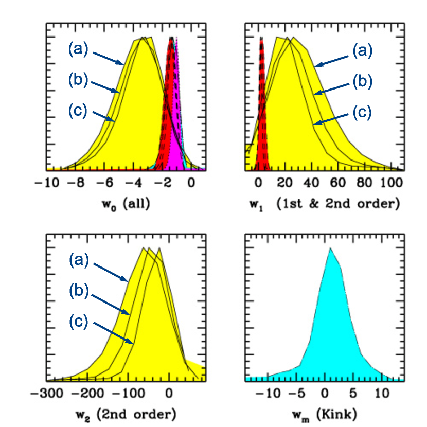
Figure 1.— Expansion order is more important than parametrisation. 1-d marginalised likelihoods for the different classes of parametrisations. The narrow curves are the linear likelihoods (constant $w_{DE}$, $n=0$, is dotted, first-order expansions, $n\leq 1$, are dashed). The solid lines show the likelihoods at second-order ($n\leq 2$) and are much wider due to degeneracies and the absence of a lower-bound on $w$ for $z\geq 1$. The curves correspond to expansions in (a) scale-factor, (b) log and (c) redshift respectively. Finally the 1-d likelihood for $w_{m}$ of the Kink is shown (dot-dashed) and exhibits strongly non-Gaussian wings that extend to very large values of $|w_{m}|$. For definition of the order of the expansion see eq. (1).

In order to be conservative we use only the gold sample of (Riess et al., 2004), containing $157$ data points. In our analysis we assume a flat Friedmann-Lemaitre-Robertson-Walker (FLRW) universe. The assumption of flatness is required to achieve reasonable error bars (c.f. Kunz and Bassett 2004; Dicus and Repko 2004). Fortunately this is now a data-driven assumption and particularly harmless for this study since we are primarily interested in testing compressions rather than deriving constraints. We will also assume the prior $\Omega_{m}=0.27\pm 0.04$. This can be justified from CMB data, as shown in Kunz et al. (2003) and Corasaniti et al. (2004), the best-fit values for background FLRW parameters are not affected strongly by dark energy dynamics.

The luminosity distance is given by

$$d_{L}(z)=(1+z)\int_{0}^{z}\frac{dz^{\prime}}{H(z^{\prime})},$$ (7)

and

$$H(z)=H_{0}[\Omega_{m}(1+z)^{3}+(1-\Omega_{m})f(z)]^{1/2},$$ (8)

where $f(z)$ is the solution to the continuity equation

$$f(z)=\exp{\left(3\int_{0}^{z}\frac{1+w_{DE}(z^{\prime})}{1+z^{\prime}}dz^{\prime}\right)}.$$ (9)

Our analysis methods are described in detail in Corasaniti et al. (2004). We use a Markov-Chain Monte Carlo code to find the constraints on the dark energy parameters for each parametrisation. As usual we marginalise analytically over the normalisation of $d_{L}$ which takes care of the Hubble constant as well, leaving $\Omega_{m}$ as the only remaining parameter apart from those describing the equation of state.

Figure 1 shows the marginalised one-dimensional likelihoods for the parameters of the dark energy compressions. The main point of that figure is that the various parametrisations have similar likelihoods at the same order, but that the likelihoods at different orders are completely different. Here by order we mean the maximum value of $n$ in eq. (1). Hence “linear” or “first-order” ($n\leq 1$) refers to the standard two-parameter expansions with only $w_{0},w_{1}$ non-zero, while 2nd-order corresponds to $n\leq 2$ and has non-zero $w_{2}$.

The best-fit values and $1\sigma$ errors for the first-order redshift, scale factor and logarithmic parametrisations are given in table 1; these are consistent with those found in (Feng et al. 2004; Gong 2004).

Table 1Best fit values and $1\sigma$ confidence intervals at linear order ($n\leq 1$).

	$w_{0}$	$w_{1}$
Redshift	$-1.30\pm_{0.52}^{0.43}$	$1.57\pm_{1.41}^{1.58}$
Scale-factor	$-1.48\pm_{0.64}^{0.57}$	$3.11\pm_{3.12}^{2.98}$
Log	$-1.39\pm_{0.57}^{0.50}$	$2.25\pm_{2.15}^{2.19}$

We infer the ’maximised’ limits on the redshift dependence of the equation of state by computing for a given parametrisation the highest and lowest $w_{DE}(z)$ for the models in the chains with $\chi^{2}<\chi_{min}^{2}+4$. Models with $w(z)$ outside those limits are therefore expected to be “bad” fits to the SN-Ia data. We plot the result in Figure 2. For the two-parameter models, the limits are very similar to those obtained by marginalising over all other parameters, as is expected since they are nearly Gaussian. We have also checked that they coincide with limits from Gaussian error propagation.

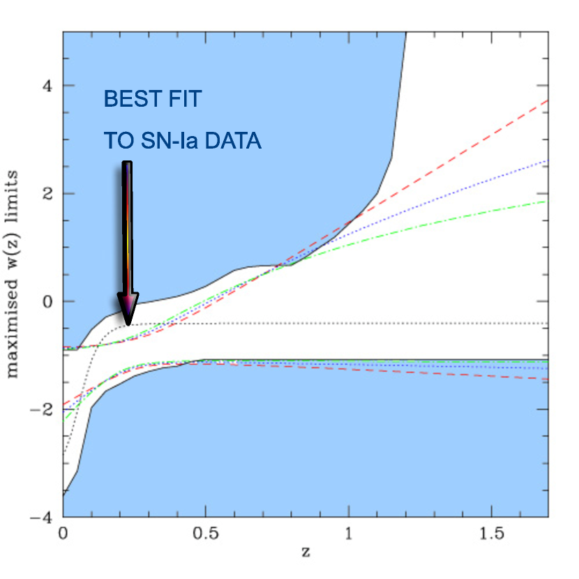
Figure 2.— Parametrisations struggle with rapid evolution. Maximised limits on $w_{DE}(z)$ for the redshift (red dashed line), scale-factor (green dash-dotted), logarithmic (blue dotted) and Kink (solid black line) parametrisations. The best-fit kink solution passes well outside the limits of all the parametrisations (except for the kink) both at $z\sim 0$ and at $z\sim 0.2$, showing their inability to capture rapid dynamics which leads to their incorrectly ruling it out.

We now discuss the constraints derived from the Kink formula, Eq. (6). The best fit to the data has a $\chi^{2}=172.6$ and is characterized by: $w_{0}=-2.85$, $w_{m}=-0.41$, $a_{t}=0.94$ and $\log({\Delta})=-1.52$, corresponding to a rapidly varying equation of state with a transition from $w_{m}$ to $w_{0}$ at $z_{t}=0.1$. This best-fit is shown in figure 2 and clearly exits the $2\sigma$ limits from the two-parameter compressions, first from below at $z\sim 0$ and then from above, at $z\sim 0.2$. This graphically illustrates the limitations of the standard parametrisations and shows how they artificially rule out models which should give the strongest signals for dark energy dynamics Corasaniti et al. (2003).

Although the Kink formula is by construction everywhere under control, the dependence on its parameters is highly non-linear so the peaks of the marginalised likelihood distributions do not match the values of the best fit model. In fact the peaks of the $1$-dimensional marginalised likelihoods are shifted with the respect to the best fit values after marginalising. Hence the marginalised likelihoods do not coincide with the maximized ones, as they would if the likelihood distributions were Gaussian.

It is not just one good fit to the data which violates the $2\sigma$ limits of all the two-parameter compressions either. For instance, the model with $w_{0}=-1.46$, $w_{m}=0.16$, $a_{t}=0.88$ and $\log{(\Delta)}=-0.7$ has $\chi^{2}=173.9$, while the model with $w_{0}=-1.11$, $w_{m}=6.13$, $a_{t}=0.40$ and $\log{(\Delta)}=-.98$, has $\chi^{2}=175.9$. Both are excellent fits to the data but are supposedly ruled out by the $n\leq 1$, linear redshift, scale-factor and logarithmic parametrisations of equations (3-5).

The conclusion that rapid evolution of dark energy is ruled out by current data is therefore a ‘gauge’ artifact. We have shown that rapid variations of the dark energy equation of state are perfectly consistent with, and in fact provide better fits to the Gold sample than do models without rapid transitions. This conclusion remains even after including CMB and large scale structure data (Corasaniti et al. 2004).

The pathological behaviour of ruling out models which are very good fits to the data can be rectified by the inclusion of higher order terms, $n\geq 2$. Indeed, since the data allow $w_{1}$ to be large in all cases, higher order terms in the redshift, scale-factor and Log expansions cannot be neglected. Therefore we have extended our analysis in order to include second order corrections $(n\leq 2)$ to Eq. (3)-(5).

Comparing the yellow likelihoods in Figure 1 with the red ones we see that by the allowed values of $w_{0}$ are shifted significantly towards more negative values, consistent with, but broader than the kink confidence interval. Secondly huge values of $w_{1}\sim 50$ and $w_{2}\sim-100$ are consistent with the data. This suggests that strong dark energy dynamics is not ruled out and that higher order terms must be taken into account. As mentioned in the introduction, this comes from the fact that $w_{1}$ and $w_{2}$ are strongly degenerate in all cases and that there is no lower bound on $w$ at $z>1$, illustrating the huge effect of imposing the weak energy condition $w\geq-1$.

In this case we have both a lower bound (from the weak energy condition) and an upper bound (from the data) on $w$. As the second order parametrisations are described by a parabola in their respective expansion variables, they end up being strongly constrained.

On the other hand, we have also considered much higher order ($n\leq 6$), and found that severe internal degeneracies lead to finely balanced coefficients. Thus a Taylor expansion in $z$ becomes very unstable at high redshift, and even expansions in $1-a$ can hardly be called “under control” anywhere since the expansion coefficients become of order $10^{3}$.

3.1. Model selection with Information Criteria and the Bayesian Evidence

In table 2 we report the values of the $\chi^{2}$ for the best fit models of each parametrisation. As we can see the four-parameter Kink formula has the lowest $\chi^{2}$, followed by the scale-factor, the logarithmic and redshift parametrisation. Accounting for second order terms ($n\leq 2$) in the expansions provide fits even better than the best Kink parametrisation which is non-trivial since they have one less parameter, although now the allowed parameter space volume is huge.

At this point we can ask how many parameters are actually necessary to describe the dark energy with current SN-Ia data? Following Liddle (2004), we compute the Akaike information criterion (Akaike 1974)

$$AIC=-2\ln{\mathcal{L}}+2k$$ (10)

and Bayesian information criterion (Schwarz 1978)

$$BIC=-2\ln{\mathcal{L}+k\ln{N}},$$ (11)

where $\mathcal{L}$ is the maximum likelihood, $k$ is the number of model parameters and $N$ is the number of data points. We also compute the Bayesian evidence $E$ (Sivia 1996; Saini, Weller and Bridle 2004), both with thermodynamic integration and nested sampling (Skilling 2004). It is worth noting that fully degenerate parameters do not contribute to the Evidence, so that specifically the Kink model is less disfavored than the number of parameters suggests naively. For the same reason we find that $E$ grows very slowly when going to even higher order in the expansion-type parametrisations, although these cases are already disfavored by Bayesian statistics. The preferred parametrisation is $\Lambda$CDM – it is indeed remarkable that a model with a single free parameter fits the data so well.

Table 2Bayesian Evidence, BIC, AIC and $\chi^{2}$ values of best fit for different parametrisations. $k$ is the total number of fitting parameters which include the dark energy density $\Omega_{DE}$

model	k	$\chi^{2}$	BIC	AIC	$-\ln(E)$
$\Lambda$CDM	1	177.6	182.7	179.6	93
w=const	2	177.6	187.7	181.6	96
linear	3	174.5	189.7	180.5	99
logarithmic	3	174.2	189.4	180.2	98
scale factor	3	174.0	189.2	180.0	98
quadratic	4	172.1	192.3	180.1	100
logarithmic II	4	172.2	192.4	180.2	100
scale factor II	4	172.3	192.5	180.3	99
Kink	5	172.6	197.9	182.6	96

4. When did acceleration begin?

One of the key characteristics of dynamical dark energy is that the redshift at which the universe begins accelerating, $z_{acc}$, is characteristically different from that in $\Lambda$CDM with the same $\Omega_{DE}$ today. This is manifest in the CMB as a modified integrated Sachs-Wolfe effect (Bassett et al., 2002; Corasaniti et al., 2003) which is degenerate with reionisation (Corasaniti et al., 2004). The SN-Ia offer the possibility to break this degeneracy and therefore it is crucial to use a parametrisation that can accurately estimate $z_{acc}$ without bias. Using a simple linear expansion of the deceleration parameter $q$, Riess et al. (2004) estimated $z_{acc}=0.46\pm 0.13$. Here we compare the predictions of the various parametrisations for $z_{acc}$. The 1d likelihoods for $z_{acc}$ are shown in Figure 3 and in table 3 we report the confidence intervals.

Table 3Best fit values and $1\sigma$ confidence intervals on $z_{acc}$ at linear order ($n\leq 1$).

Model	$z_{acc}$	Model	$z_{acc}$
$\Lambda$CDM	$0.66\pm_{0.11}^{0.11}$	$w=$ const.	$0.36\pm_{0.04}^{0.25}$
Linear in $z$	$0.14\pm_{0.05}^{0.14}$	Log	$0.38\pm_{0.08}^{0.42}$
Scale-Factor	$0.59\pm_{0.21}^{8.91}$	Kink	$0.45\pm_{0.44}^{0.53}$

We have two main points. First, all of the parametrisations predict different best-fit values and $1\sigma$ error bars for $z_{acc}$, ranging from $z_{acc}=0.14$ for the redshift expansion to $z_{acc}=0.59$ for the scale-factor expansion (see also Dicus and Repko 2004). The logarithmic, constant and Kink parametrisations all have similar best-fits, but the first two have overly narrow error bars relative to the Kink predictions. The largest error bars correspond to the scale-factor expansion, eq. (4).

Given the importance of accurately estimating $z_{acc}$ this variance forcefully argues for the need to go beyond two-dimensional parametrisations in handling future, high-quality data.

As a second point it is interesting that the best-fits for $z_{acc}$ for all the parametrisations are lower than in the $\Lambda$CDM model. This may be novel evidence for dark energy dynamics. We leave this issue for future work.

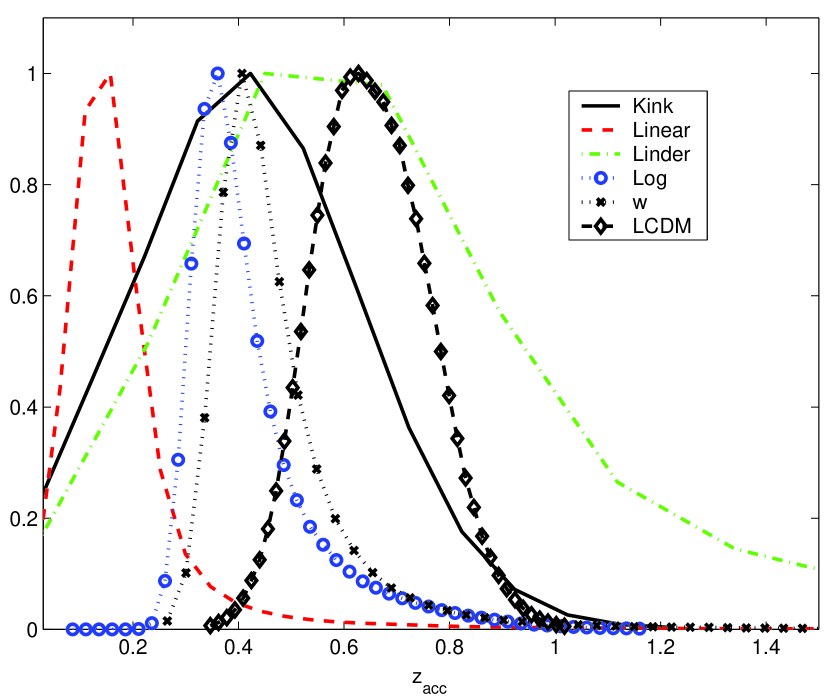
Figure 3.— When did acceleration begin? The marginalised 1d likelihood for $z_{acc}$ as estimated from the same SN-Ia data for each of the various dark energy parametrisations. The wide variance casts doubt on their usefulness. All of them peak at a lower $z_{acc}$ than in the standard $\Lambda$CDM, perhaps giving novel evidence for dark energy dynamics. Only the scale-factor expansion, eq. (4) shares significant overlap with $\Lambda$CDM, but that is expected since the transition is typically slow in that parametrisation.

5. Conclusions

This Letter shows the limitations of standard one and two-parameter compressions of the infinite dimensional space of dark energy models. We have highlighted the dangers in using constraints derived using these parametrisations, particularly regarding the possibility of rapid evolution in the dark energy, which none of the standard compressions can follow, and in defining allowed regions of parameter space which are completely wrong in the case where the weak energy condition ($w>-1$) is not imposed.

Rapid evolution provides a superlative fit to current SN-Ia data (as measured by $\chi^{2}$), despite claims to the contrary in the literature which were based on two-parameter compressions. Indeed, all of the two-parameter expansions we studied wrongly rule out such rapid evolution at $2\sigma$ or more. This is extremely damning evidence, especially since these compressions are typically used in the planning for the next-generation experiments which will provide data of significantly higher quality. In addition, the standard parametrisations also miss the fact that $w$ has no lower-bound at $z>1$ if the weak energy condition is not imposed, artifically cutting-out vast swaths of parameter space due to their innate limitations.

Further problems occur in estimating the redshift at which the universe began accelerating, $z_{acc}$. There is a nearly 300% variation in the best-fit for $z_{acc}$, depending on parametrisation. Interestingly, all the tested parametrisations gave best-fits for $z_{acc}$ below that of $\Lambda$CDM, providing unusual cross-parametrisation evidence for dark energy dynamics. Nevertheless, use of the Bayesian information criteria for model selection prefers the cosmological constant over the other models which remains the model to beat.

The severe inadequacy of the standard two-parameter expansions lead us to consider higher-order terms ($n\geq 2$) with one of more extra parameters, e.g. $w_{2}$. While this brings the rapid evolution models within the allowed region of parameter space it leads to severe degeneracies (see figure 1) which may make the parametrisations impotent for constraining the space of theoretical dark energy models, particularly when $w<-1$.

For completeness we have also compared four standard parametrisations against a test-bed of quintessence models (Appendix) and found that while the kink and scale-factor expansion are excellent, the expansions in $z$ and $\log(1+z)$ can lead to large errors for $z\geq 1$.

We conclude that confidence intervals inferred from standard two-parameter expansions often do not deserve that name and are typically untrustworthy, even with current data. The wealth and quality of dark energy data we will aquire over the next decade will demand significantly better performance.

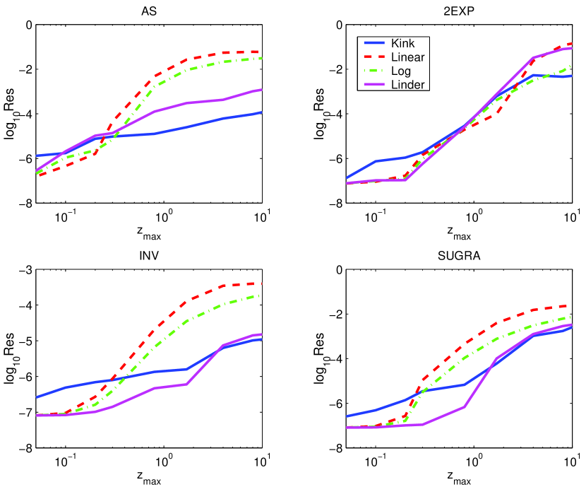
Figure 4.— Plot showing the mean quadratic error of the best-fit, eq. (5), to the different quintessence models as function of $z_{max}$ for each parametrisation for $n\leq 1$. At $z\sim 1$ the expansion to first order in $z$ (‘redshift’) and $\log(1+z)$ (‘logarithmic’) typically show errors around 10% while the kink and scale-factor parametrisations have errors typically at the 1% level at $z\sim 1$.

Our test-bed suite of models is: the Albrecht-Skordis model (Albrecht and Skordis 2001),

$$V(Q)=M^{4}e^{-\alpha Q}[(Q-A)^{2}+B]^{s/2},$$ (1)

with $\alpha=5$, $A=54.5$, $B=0.01$ and $s=5$; the Two Exponential potential (Barreiro, Copeland and Nunes 2000),

$$V(Q)=M^{4}(e^{-\alpha Q}+e^{-\beta Q}),$$ (2)

with slopes $\alpha=-9$ and $\beta=2$; the inverse power-law potential (Ratra and Peebles 1988),

$$V(Q)=M^{4+\alpha}/Q^{\alpha},$$ (3)

with $\alpha=0.6$; the Supergravity (SUGRA) inspired model (Brax and Martin 1999),

$$V(Q)=M^{4}e^{-Q^{2}/2}/Q^{\alpha},$$ (4)

with $\alpha=6$. For the kink and each two-parameter expansion ($n\leq 1$) we compute the best-fit (using an MCMC search) to the different quintessence models in the redshift range $0<z<z_{max}$ and plot the average residual quadratic errors as a function of $z_{max}$, as shown in Figure 4, where

$$Res=\frac{1}{N_{z}}\sum_{i=1}^{N_{z}}(w_{Q}(z_{i})-w_{par}^{best}(z_{i}))^{2},$$ (5)

with $N_{z}$ the total number of equally spaced bins in the range $[0,z_{max}]$, and we have chosen $N_{z}=1000$. Comparing the residuals indicates how well each formula reproduces a given quintessence model as function of the redshift interval. For $z_{max}\geq 0.3$, the Kink and scale-factor formulae provide best-fits which are at least one order of magnitude better than the redshift and logarithmic expansions, except perhaps in the Two-Exponential case.

Only for $z_{max}<0.3$ are the residuals of the redshift and logarithmic formulas of the same order as those of the other parametrisations. This is easy to understand from Fig. (2). The best-fit solution is almost perfectly linear for $z<0.1$ but then suddenly deviates. A linear fit will be excellent until $z\sim 0.1$, after which it rapidly becomes bad.

We do not consider the case of constant $w$ which can at best fit the average value of $w(z)$ and whose errors are expected to be the worst.

References

- (1) Akaike, H., 1974, IEEE Trans. Auto. Control, 19, 716.
- (2) Alam, U., Sahni, V, Saini, T.D. and Starobinsky, A.A. 2003, astro-ph/0311364.
- (3) Albrecht, A. and Skordis, C. 2001, Phys. Rev. D64, 023514, astro-ph/9908085.
- (4) Barreiro, T., Copeland, E.J. and Nunes, N.J. 2000, Phys. Rev. D61, 127301, astro-ph/9910214.
- Bassett et al. (2002) Bassett, B.A., Kunz, M., Silk, J. and Ungarelli, C. 2002, MNRAS336, 1217, astro-ph/0203383.
- Bassett et al. (2003) Bassett, A. M., Kunz, M., Parkinson, D. and Ungarelli, C., 2003, Phys. Rev. D68, 043504, astro-ph/0211303.
- (7) Bassett, B. A. and Kunz, M., 2004, Phys. Rev. D69, 101305, astro-ph/0312443.
- (8) Brax, P. and Martin, J. 1999, Phys. Lett. B468, 40, astro-ph/9905040.
- (9) Caldwell R. R. and Doran, M., 2004, Phys. Rev. D 69, 103517
- (10) Chevallier, M. and, Polarski, D. 2001, Int. J. Mod. Phys. D10, 213, gr-qc/0009008.
- Corasaniti and Copeland (2002) Corasaniti, P.S. and Copeland, E.J. 2002, Phys. Rev. D67, 063521, astro-ph/0205544.
- Corasaniti et al. (2003) Corasaniti, P.S., Bassett, B.A., Copeland, E.J. and Ungarelli, C. 2003, Phys. Rev. Lett. 90, 091393, astro-ph/0210209.
- Corasaniti et al. (2004) Corasaniti, P.S., Kunz, M., Parkinson, D., Copeland, E.J. and Bassett, B.A., 2004, astro-ph/0406608.
- (14) Dicus, D.A. and Repko, W.W. 2004, astro-ph/0407094.
- Efstathiou (1999) Efstathiou, G. 1999, MNRAS303, L47, astro-ph/9812226.
- Feng et al. (2004) Feng, B., Wang, X.-L. and Zhang, X.-M. 2004, astro-ph/0404224.
- Gong (2004) Gong, Y. 2004, astro-ph/0405446.
- Hu (2004) Hu, W. and Jain, B., (2003) astro-ph/0312395.
- Huterer and Turner (2001) Huterer, D. and Turner, M.S. 2001, Phys.Rev. D64, astro-ph/0012510.
- Huterer and Starkmann (2003) Huterer, D. and Starkman, M.S. 2003, Phys. Rev. Lett. 90, 031301, astro-ph/0207517.
- (21) Huterer, D. and Cooray, A.R. 2004, astro-ph/0404062.
- Jassal et al. (2004) Jassal, H.K., Bagla, J.S. and Padmanabhan, T. 2004, astro-ph/0404378.
- Jonsson et al. (2004) Jonsson, J, Goobar, A., Amanullah, R. and Bergstrom, L. 2004, astro-ph/0404468.
- (24) Kunz, M., Corasaniti, P.S., Parkinson, D. and Copeland, J.C. 2003, astro-ph/0307346.
- (25) Kunz, M. and Bassett, B. A., 2004, astro-ph/0406013.
- Liddle (2004) Liddle, A.R. 2004, astro-ph/0401198.
- Linder (2003) Linder, E.V. 2003, Phys. Rev. Lett. 90, 91301, astro-ph/0402503.
- Linder (2004) Linder, E.V. 2004, astro-ph/0402503.
- Maor et al. (2002) Maor, I., Brustein, McMahon, J. and Steinhardt, P.J. 2002, Phys. Rev. D65, 123003, astro-ph/0112526.
- Melchiorri et al. (2003) Melchiorri, A. et al., 2003, Phys. Rev. D 68, 043509.
- (31) Ratra, B. and Peebles, P.J.E. 1988, Phys. Rev. D37, 3406.
- Riess et al. (2004) Riess, A. et al. 2004, astro-ph/0402512.
- (33) Saini, T.D., Weller, J. and Bridle, S. L., 2004, Mon. Not. Roy. Astron. Soc. 348, 603
- (34) Schwarz, G. 1978, Annals of Statistics, 5, 461.
- (35) Sivia, D. S. 1996, Data Analysis: A Bayesian Tutorial (New York: Oxford Univ. Press)
- (36) Skilling, J. 2004, http://www.inference.phy.cam.ac.uk/bayesys/
- Virey et al. (2004) J. M. Virey, P. Taxil, A. Tilquin, A. Ealet, D. Fouchez and C. Tao, arXiv:astro-ph/0403285.
- Wang and Freese (2004) Wang, Y., F. and Freese, K. 2004, astro-ph/0402208.
- Wang and Tegmark (2004) Wang, Y., and Tegmark, M., 2004, Phys. Rev. Lett., 92, 241302
- Weller and Albrecht (2002) Weller, J. and Albrecht, A. 2002, Phys. Rev.D65, astro-ph/0106079.
- Wetterich (2004) Wetterich, C. 2004, astro-ph/0403289.