C II Radiative Cooling of the Diffuse Gas in the Milky Way

Abstract

The heating and cooling of the interstellar medium (ISM) allow the gas in the ISM to coexist at very different temperatures in thermal pressure equilibrium. The rate at which the gas cools or heats is therefore a fundamental ingredient for any theory of the ISM. The heating cannot be directly determined, but the cooling can be inferred from observations of C II*, which is an important coolant in different environments. The amount of cooling can be measured through either the intensity of the 157.7 $\micron$ [C II] emission line or the C II* absorption lines at 1037.018 Å and 1335.708 Å, observable with the Far Ultraviolet Spectroscopic Explorer and the Space Telescope Imaging Spectrograph onboard of the Hubble Space Telescope, respectively. We present the results of a survey of these far-UV absorption lines in 43 objects situated at $\mid\!b\!\mid\gtrsim 30\arcdeg$. Measured column densities of C II*, S II, P II, and Fe II are combined with H I 21-cm emission measurements to derive the cooling rates (per H atom using H I and per nucleon using S II), and to analyze the ionization structure, the depletion, and metallicity content of the low-, intermediate-, and high-velocity clouds (LVCs, IVCs, and HVCs) along the different sightlines. Based on the depletion and the ionization structure, the LVCs, IVCs, and HVCs consist mostly of warm neutral and ionized clouds.

For the LVCs, the mean cooling rate in erg s^-1 per H atom is $-25.70^{+0.19}_{-0.36}$ dex ($1\sigma$ dispersion). With a smaller sample and a bias toward high H I column density, the cooling rate per nucleon is similar. The corresponding total Galactic C II luminosity in the 157.7 $\micron$ emission line is $L\sim 2.6\times 10^{7}$ L_⊙. Combining $N($C II*) with the intensity of H$\alpha$ emission, we derive that $\sim$50% of the C II* radiative cooling comes from the warm ionized medium (WIM). The large dispersion in the cooling rates is certainly due to a combination of differences in the ionization fraction, in the dust-to-gas fraction, and physical conditions between sightlines. For the IVC IV Arch at $z\!\sim\!1$ kpc we find that on average the cooling is a factor 2 lower than in the LVCs that probe gas at lower $z$. For an HVC (Complex C, at $z>6$ kpc) we find the much lower rate of $-26.99\,^{+0.21}_{-0.53}$ dex, similar to the rates observed in a sample of damped Ly$\alpha$ absorber systems (DLAs). The fact that in the Milky Way a substantial fraction of the C II cooling comes from the WIM implies that this is probably also true in the DLAs.

We also derive the electron density, assuming a typical temperature of the warm gas of 6000 K: For the LVCs, $\langle n_{e}\rangle=0.08\pm 0.04$ cm^-3 and for the IV Arch, $\langle n_{e}\rangle=0.03\pm 0.01$ cm^-3 ($1\sigma$ dispersion).

Finally, we measured the column densities $N($S II) and $N($P II) in many sightlines, and confirm that sulphur appears undepleted in the ISM. Phosphorus becomes progressively more deficient when $\log N($H I$)>19.7$ dex, which can either mean that P becomes more depleted into dust as more neutral gas is present, or that P is always depleted by about $-0.3$ dex, but the higher value of P II at lower H I column density indicates the need for an ionization correction.

1 Introduction

The diffuse interstellar medium (ISM) consists of several coexisting gas-phases: a cold neutral medium (CNM) at $T\sim 100$ K, a warm neutral or ionized diffuse medium (WNM, WIM) at $T\sim 6\times 10^{3}-10^{4}$ K, and a hot, ionized phase at $T\sim 10^{6}$ K. In a multi-phase medium, the CNM and the WNM can coexist in thermal pressure equilibrium at very different temperatures because of the heating and the cooling properties of the gas (Field, Goldsmith, & Habing, 1969; McKee & Ostriker, 1977; McKee, 1995; Wolfire et al., 1995). The heating of the gas can not be directly estimated, but can be inferred from C II radiative cooling (Pottasch, Wesselius, & van Duinen, 1979) because the 157.7 $\micron$ emission-line transition of C II is a major coolant of the interstellar gas in a wide range of environments (Dalgarno & McCray, 1972; Heiles, 1994; Wolfire et al., 1995, 2003, and references therein). C II 157.7 $\micron$ emission is a major coolant because: (i) After oxygen, carbon is the most abundant gas phase metal in the Universe; (ii) its singly-ionized form is the most abundant ionization stage in the diffuse CNM, WNM, and WIM; (iii) the ²P_3/2 fine-structure state of C II is easily excited ($h\nu/k=91$ K) under typical conditions in the CNM, WNM, and WIM. The amount of C II radiative cooling can be determined either by measuring the C II* absorption lines originating in the ²P_3/2 level at 1037.018 Å and 1335.708 Å in the far-ultraviolet (FUV) (e.g., Pottasch, Wesselius, & van Duinen, 1979; Grewing, 1981; Gry, Lequeux, & Boulanger, 1992) or by measuring the [C II] ²P${}_{3/2}\rightarrow^{2}$P_1/2 157.7 $\micron$ line intensity in the far infra-red (FIR) (e.g., Shibai et al., 1991; Bock et al., 1993; Bennett et al., 1994). Not only is the C II radiative cooling important for understanding the energy budget of the ISM, but it has also been used to evaluate the star formation rate (SFR) in nearby star-forming galaxies (Pierini et al., 2001) and in damped Ly $\alpha$ systems (Wolfe, Prochaska, & Gawiser, 2003; Wolfe, Gawiser, & Prochaska, 2003).

In our Galaxy, there are many FUV C II* measurements for gas within a few hundred pc (Gry, Lequeux, & Boulanger, 1992; Lehner et al., 2003), but there are only a few observations of more distant gas at high galactic-latitudes (e.g, Savage et al., 1993; Spitzer & Fitzpatrick, 1993, 1995; Savage & Sembach, 1996a; Fitzpatrick & Spitzer, 1997). Recent observations of a large number ($>100$) of high Galactic latitude stars and extragalactic objects with the Space Telescope Imaging Spectrograph (STIS) onboard of the Hubble Space Telescope (HST) and the Far-Ultraviolet Spectroscopic Explorer (FUSE) now make possible an extensive study of the C II radiative cooling in the gas of our Galaxy at high Galactic latitudes.

We present the cooling rate inferred from the C II* absorption lines at 1335.708 Å and/or 1037.018 Å (available in the STIS and FUSE wavelength bands, respectively) measured in the FUV continuum of 43 objects at $\mid\!b\!\mid\gtrsim 30\arcdeg$. The cooling rates of the low-, intermediate- and high-velocity gas in these sightlines are derived. In § 2, we discuss the physical processes and the assumptions that are necessary to derive the cooling rate using the ratios of the column densities of C II* to H I and S II. § 3 presents the observations, and § 4 the analysis. In particular, we discuss the use of a curve-of-growth analysis of the Fe II absorption lines to derive reliable column densities for the other ions. In § 5, we discuss the physical properties of the clouds encountered in this work. The cooling rates are presented and analyzed in § 6, where we also compare our results to more local FUV measurements and FIR studies of the Milky Way. In § 7, we present some direct implications of the C II* absorption, including the origin of C II* absorption at high Galactic latitude (§ 7.1), the total C II integrated cooling rate of the Galaxy in the warm neutral and warm ionized gas (§ 7.2), the electron density (§ 7.3), and the comparison of our survey to high redshift studies (§ 7.4). Finally we summarize our results in § 8.

2 Electron Density and C II Cooling Rate from Measurements of $N($C II*)

The ground state of C II is split into two fine structure levels, designated (2p) ²P_3/2 and (2p) ²P_1/2. Transitions from the ²P_1/2 ground state to the ²D and ²S levels produce absorption lines at 1334.532 Å and 1036.337 Å, respectively, while absorption from the excited ²P_3/2 state produces lines at 1335.708 Å (with the oscillator strength $f=1.28\times 10^{-1}$) and 1037.018 Å ($f=1.18\times 10^{-1}$). These transitions are directly observable with STIS and FUSE, respectively. In this work, the adopted atomic parameters and in particular the oscillator strengths are from the updated atomic compilation of Morton (2003), except as otherwise stated.

The population of the fine-structure levels of C II is governed by the equation of excitation equilibrium:

$$n({\rm C}^{+*})[A_{21}+n_{e}\gamma_{21}(e)+n({\rm H})\gamma_{21}({\rm H})]=n({\rm C}^{+})[n_{e}\gamma_{12}(e)+n({\rm H})\gamma_{12}({\rm H})]$$ (1)

where $\gamma$ are the excitation (“12”) and deexcitation (“21”) rates due to collisions with electrons and neutral hydrogen atoms (Spitzer, 1978), the radiative-decay probability for the upper level is $A_{21}=2.29\times 10^{-6}$ s^-1 (Nussbaumer & Storey, 1981), and $n$ is the number density in cm^-3 of the electron ($n_{e}$) or a given species $X$ ($n(X)$) with $n({\rm C}^{+*})$ referring to the ²P_3/2 state and $n({\rm C^{+}})$ to the ²P_1/2 state. The collisional excitation rate for electron collisions is given by (Spitzer, 1978; Osterbrock, 1989),

$$\gamma_{12}(e)=\frac{8.63\times 10^{-6}}{g_{1}\sqrt{T}}\Omega_{12}e^{\frac{-E_{12}}{kT}}\,{\rm cm^{3}\,s^{-1}}\,;$$ (2)

where, for C II, $g_{1}=2$, $E_{12}/k=91.7$ K, and the collision strength $\Omega_{12}$ varies from 1.87 to 2.90 when the temperature varies from $10^{3}$ to $10^{4}$ K (Hayes & Nussbaumer, 1984). The collisional excitation and deexcitation rates are related through $\gamma_{12}=(g_{2}/g_{1})\exp(-h\nu_{12}/kT)\gamma_{21}$ (where $g_{2}=4$). The collisional deexcitation rate for H atoms is $\gamma_{12}({\rm H})\sim 10^{-9}$ cm³ s^-1, roughly constant with T (York & Kinahan, 1979; Hollenbach & McKee, 1989). We neglect the collisional excitation with protons because it is inhibited by the Coulomb repulsion when $T<4\times 10^{4}$ K (Bahcall & Wolf, 1968). We will argue in § 5 that our sightlines are not composed of CNM but of a mixture of WNM and WIM, so that collisions between H₂ and C II are also negligible. From the ratio $n_{e}\gamma_{12}(e)/(n({\rm H})\gamma_{12}({\rm H}))\approx 100n_{e}/n({\rm H})T_{4}^{-0.5}$ ($T_{4}=T/10^{4}$), one can readily see that collisional excitations with neutral hydrogen atoms can be neglected for $n_{e}/n({\rm H})>0.01$. That is for a typical $n_{e}\approx 0.08$ cm^-3 (see § 7.3), $n({\rm H})\lesssim 10$ cm^-3. At higher $n({\rm H})$ our sightlines would be dominated by clouds with $T<100$ K, but we discuss in § 5 that this can not be the case, and thus we can neglect collisional excitations by hydrogen for our sightlines. C II radiative cooling appears to be also more effective in the WIM than the pure WNM: Wolfire et al. (1995) predicted a factor $\sim$10 times higher cooling rate per hydrogen nucleus in the WIM than in the WNM.

Thus, in the warm neutral and ionized gas, the upper level of C II is excited by collisions with electrons and followed by the spontaneous emission of a 157.7 $\micron$ photon when the ion decays to the ground state. Eq. 1 can then be simplified to:

$$n_{e}\simeq 0.531\frac{\sqrt{T}}{\Omega_{12}}e^{\frac{91.7{\rm K}}{T}}\,\frac{N({\rm C}^{+*})}{N({\rm C}^{+})}\,{\rm cm}^{-3}\,,$$ (3)

where we have approximated $n($C II*$)/n($C II) by $N($C II*$)/N($C II). At $T=6000$ K, $\Omega_{12}=2.73$ (Hayes & Nussbaumer, 1984) and $n_{e}\simeq 15.29N({\rm C}^{+*})/N({\rm C}^{+})$ cm^-3.

The energy loss from spontaneous emission at 157.7 $\micron$ is in the warm-ionized and neutral-diffuse gas, in which the electron and hydrogen deexcitations are negligible compared to the spontaneous radiative deexcitation ($n_{e}\lesssim 1$ cm^-3 and $n_{e}/n({\rm H})>0.01$):

$$\Lambda({\rm C}^{+})=h\nu_{21}A_{21}n({\rm C}^{+*})=2.89\times 10^{-20}n({\rm C}^{+*})\,\,{\rm erg}\,{\rm s}^{-1}\,{\rm cm}^{-3}\,.$$

Note that this equation can be related to the electron density and temperature via Eq. 3, $\Lambda({\rm C}^{+})\propto n_{e}n({\rm C}^{+})/\sqrt{T}$.

To compare the cooling in different directions in the Galaxy, it is useful to calculate both the cooling per neutral hydrogen atom or per nucleon along the line of sight. We therefore define the cooling per neutral H atom to be:

$$l_{c}\tbond\frac{\int\Lambda({\rm C}^{+})ds}{\int n({\rm H}^{0})ds}=2.89\times 10^{-20}\frac{N({\rm C}^{+*})}{N({\rm H}^{0})}\,\,{\rm erg}\,{\rm s}^{-1}\,({\rm H\,atom})^{-1}\,.$$ (4)

To estimate the total hydrogen column density along the sightlines, we use the ion S II as a proxy of H I+H II, assuming a cosmic (meteoric) abundance for sulfur (S/H)_⊙ of $10^{-4.80}$ (Grevesse & Sauval, 1998). S is not depleted (Savage & Sembach, 1996a, and references therein), and its second ionization potential of 23.3 eV is high enough to ensure that S II is the dominant ion in both neutral and partially-ionized diffuse gas. From a study of H$\alpha$ and [S II] emission lines, Haffner, Reynolds, & Tufte (1999) find that typically S II/S $\sim 0.3$ to 0.8 in the WIM. We therefore have $N($H I$)+N($H II$)=({\rm H}/{\rm S})_{\odot}N($S II), and thus we can derive the cooling rate per nucleon as

$$L_{c}=2.89\times 10^{-20}\frac{N({\rm C}^{+*})}{N({\rm S}^{+})}\left(\frac{{\rm S}}{{\rm H}}\right)_{\odot}\,\,{\rm erg}\,{\rm s}^{-1}\,{\rm nucleon}^{-1}\,.$$ (5)

Phosphorus is lightly depleted into dust and does not make a good proxy of H I+H II. But P can be used along with Fe to study the depletion of the gas (see § 5).

3 Observations and Data Handling

3.1 The Sample

Our sample is based primarily on a recent FUSE survey of O VI absorption toward 100 extragalactic sightlines (Wakker et al., 2003; Savage et al., 2003; Sembach et al., 2003a). We also searched the HST/STIS archive for supplementary or complementary data as well as for suitable Galactic Halo stars with known distances. While many more stars than extragalactic objects were observed with FUSE, only a few of them are at high enough galactic latitudes to avoid strong Galactic Disk H₂ contamination and have clean-enough stellar spectra for our purposes (i.e. stars with a simple stellar continuum: metal-poor stars or stars with rotationally-broadened stellar lines). The other criteria for choosing our sightlines are as follows: (1) sightlines with high-positive velocity H I resulting in the C II line overlapping the C II* line were rejected; (2) sightlines with strong H₂ lines that are blended with C II* $\lambda$1037 were rejected; (3) sightlines in which the background galaxies’ intrinsic Ly$\beta$ line interferes with C II* $\lambda$1037 were also rejected; (4) only sightlines with a signal-to-noise ratio of at least 8 per 20 ${\rm km\,s}^{-1}$ resolution element were chosen, to allow reliable measurements.

Our final sample consists of 43 objects: 35 QSOs/AGNs, 4 early-type stars, 3 post-AGB stars in globular cluster, and 1 subdwarf star. Tables 1 and 2 list the principal properties of the extragalactic and stellar objects, respectively. The distribution of the targets on the Galactic sky is shown in Fig. 1. Thirty objects are at $b>+27\arcdeg$, 13 at $b<-21\arcdeg$. All but three of our targets are situated at latitudes $\mid\!b\!\mid>30\arcdeg$ because of the large extinction (and large H₂ column density) in the galactic plane at lower latitudes.

3.2 The H I Emission Spectra

We use high spectral resolution ($\sim 1$ ${\rm km\,s}^{-1}$) H I 21-cm emission data for two reasons: (i) to get the component structure along a given a sightline; (ii) to measure H I column densities to compare to the other ions.

The H I column densities were derived by integrating the brightness temperature over the velocity ranges of the clouds, in H I observations pointed toward or near the direction of the background targets, following Wakker et al. (2001). The last column of Tables 1 and 2 lists the source of the H I data that we used: the Leiden-Dwingeloo Survey (LDS; Hartmann & Burton 1997; 35′ beam), the Villa Elisa telescope (data courtesy R. Morras; 34′ beam), the Green Bank 140-ft telescope (data courtesy E. Murphy; 21′ beam), the Jodrell Bank telescope (data courtesy R. Ryans; 12′ beam), and the Effelsberg telescope (see Wakker et al. 2001; 9′ beam). Most of these spectra were previously shown by Wakker et al. (2001).

The major advantage of using the H I emission line over the Ly $\alpha$ absorption lines is that the different clouds in the line of sight can be separated. The disadvantage is that the beam of the radio telescope is large, and thus only represents the average column density over a region near the target. If there is much small-scale structure, the average may differ substantially from the value in the precise direction toward the target. Wakker et al. (2001) studied this effect, and found that for HVCs $N($H I) measured with a half-degree radio beam can differ by up to a factor 2–3 (either way) from the value measured with a 10′ or 1′ beam. The distribution of $N($H I;36′)/$N($H I;9′) has a dispersion of about a factor 1.5, or 0.17 dex. Comparing $N($H I) measured with a 9′ beam or with a 1′ beam or through Ly $\alpha$ absorption gives a narrower range, corresponding to a factor up to $\sim$1.25, with a dispersion in the ratio of about a factor 1.15 (0.06 dex). This effect make the value of $N($H I) in the directions toward the background targets much more uncertain than would be expected from the noise in the H I data. To account for this, we use errors of 0.17 dex for LDS and VE data, 0.10 dex for Green Bank data, and 0.06 dex for Jodrell Bank and Effelsberg data, rather than the statistical errors calculated from the noise in the H I spectra.

In two cases (HD 18100 and HD 97991), we instead used the column density found from the Ly $\alpha$ absorption line because the FUV observations did not resolve the different H I clouds and the measurements of H I Ly $\alpha$ have smaller errors, because beam smearing is no longer a problem. We also note that in the few cases where there is both a Ly $\alpha$ H I column density and a 21-cm H I emission column density, the two measures are consistent (for example, vZ 1128). For sightlines where stars are used to provide the background continuum, another error could arise because the exact location of the star relative to the interstellar clouds is unknown. For the H I emission line the column density is derived between us and “infinity”, while for the absorption line the column density is derived from us to the star. However, because the stars are at high Galactic latitudes and distant, this error should remain small.

The H I emission spectra are presented in Figs. 2 and 6, where the vertical dotted lines indicate the different components obtained from the Gaussian profile fitting of the emission line. We also show in this figure the component number and its associated velocity centroid and H I column density in units of $10^{18}$ cm^-2. The component numbers appear in the last columns of Tables 3 and 4 that summarize our measurements.

3.3 HST/STIS E140M Data Reduction

Several sightlines (see last column of Tables 1 and 2) were observed with the E140M echelle mode of STIS (FUV, $1150-1730$ Å). The absorption lines used in this wavelength region are C II* $\lambda$1335 and S II $\lambda$$\lambda$1250, 1253, and 1259. The typical spectral resolution of these data is $\sim 7$ ${\rm km\,s}^{-1}$. We used the full STIS 3.5 ${\rm km\,s}^{-1}$ pixel sampling to analyse the data, except if the the signal-to-noise (S/N) ratio was less than 6 per $\sim 7.0$ ${\rm km\,s}^{-1}$ spectral resolution, we binned the data by 2 pixels.

Data were reduced within IRAF, using the stsdas packages. Standard calibration and extraction procedures were employed using the calstis stsdas version 2.2 routine.

The STIS observations were obtained in the heliocentric frame. For STIS spectra, the absolute wavelength calibration is accurate, and we thus corrected these spectra to the Local Standard of Rest (LSR) frame. Once the correction was applied, a good alignment was observed between the STIS and H I emission spectra, and no further correction was deemed necessary (see Figs. 2 and 6). However, the STIS resolution is less than the spectral resolution of the H I emission data ($\sim$1 ${\rm km\,s}^{-1}$). Hence, the measurements for several H I clouds were often combined when comparing to the STIS data. For example, in the spectra of HE 1228+0131 (see Fig. 2) the first 3 components are combined into one to compare to the UV absorption at about $-8$ ${\rm km\,s}^{-1}$, but for component 4 at $+27$ ${\rm km\,s}^{-1}$ only one component is observed in both the UV and radio spectra. The last column(s) in Tables 3 and 4 indicates the H I components used to compare to the C II* absorption line (the numbers are listed on the lower panels of Figs. 2 and 6 and follow the cloud definition of Wakker et al., 2001).

3.4 FUSE Data Reduction

The FUSE instrument consists of four channels: two optimized for the short wavelengths (SiC 1 and SiC 2; 905–1100 Å) and two optimized for longer wavelengths (LiF 1 and LiF 2; 1000–1187 Å). There is, however, overlap between the different channels, and, generally, a transition appears in at least two different channels. For example, C II* $\lambda$1037 and Fe II $\lambda$$\lambda$1055, 1063 appear in LiF 1A, LiF 2B, and SiC 1A. At $\lambda>1086$ Å, Fe II and P II can be observed in LiF 2A and LiF 1B. Note, however, that we mainly make use of LiF 1A for $\lambda=1000$–1086 Å because of the better signal and spectral resolution near the C II* $\lambda$1037 line in this channel. The other channels are used to check if there are spurious instrumental features. More complete descriptions of the design and performance of the FUSE spectrograph are given by Moos et al. (2000) and Sahnow et al. (2000). To maintain optimal spectral resolution the individual channels were not added together.

Standard processing with version 2.1.6 or higher of the calibration pipeline software was used to extract and calibrate the spectra. The software screened the data for valid photon events, removed burst events, corrected for geometrical distortions, spectral motions, satellite orbital motions, and detector background noise, and finally applied flux and wavelength calibrations. The extracted spectra associated with the separate exposures were aligned by cross-correlating the positions of interstellar absorption lines, and then combined. The combined spectra were finally rebinned by 4 pixels ($27$ mÅ or 7.8 ${\rm km\,s}^{-1}$ at 1037 Å) since the extracted data are oversampled. This provides approximately three samples per 20 ${\rm km\,s}^{-1}$ resolution element.

The FUSE  instrument does not provide an accurate absolute wavelength scale. It can be inaccurate by about 20 ${\rm km\,s}^{-1}$. However, with the latest version of pipeline, the relative wavelength scale remains accurate to better than about 5 ${\rm km\,s}^{-1}$ within a segment, as found by comparing the measured velocities of many interstellar lines within each segment. To compare C II* or P II to H I, we employed an approach for adjusting absorption-line wavelengths and velocities similar to the one described in Wakker et al. (2003), and one should refer to their paper for a more complete description of these issues. To summarize, we used the C II* absorption line along with Si II at 1020.699 Å and Ar I at 1048.220 and 1066.660 Å to compare to the H I emission spectra and hence determine the velocity shifts. These lines are not strongly saturated, so that usually the deepest absorption corresponds to the strongest H I component. We also compare the FUSE absorption profiles with STIS absorption profiles whenever possible to determine reliable velocities. The spectral resolution of FUSE is far less than that of the H I emission data. Therefore, several H I clouds were often grouped together to compare to the UV absorption lines.

4 Analysis of the UV Spectra

In § 2, we showed that C II* cooling rate in erg s^-1  per H atom is proportional to $N($C II*)$/N($H I), and the cooling rate in erg s^-1  per nucleon is proportional to $N($C II*)$/N($S II). The electron density is also directly related to these quantities (§ 2). Hence, it is essential to have a reliable estimate of the column densities of C II*, S II, and H I. We already discussed in § 3.2 how the H I 21-cm emission lines were used to align the velocities of the cloud components and to determine the H I column density. To appreciate the level of saturation of the absorption lines, we principally use a curve-of-growth method, using the Fe II lines, for which several transitions exist in the FUV range. Before making any measurements, we first need to investigate the possible interference of other lines with the absorption lines of interest in our work.

4.1 UV Absorption-Line Blending

Galactic components (including high-velocity clouds) as well as extragalactic absorbers can blend with the C II* absorption lines at 1037.018 and 1335.708 Å. The last column of Table 1 indicates which instruments provided measurements of the different lines. When both instruments provided measurements, for C II* the comparison of the two transitions allows us to know directly if a line is contaminated. For the final result we only kept the best-quality data (usually from STIS, except if the S/N ratio was not good enough). We rejected any sightlines showing serious blending by IGM absorption or high-velocity C II.

The major contaminant of the C II* $\lambda$1037 line is the Lyman 5–0 R(1) line of H₂ at 1037.149 Å, which is at $+38$ ${\rm km\,s}^{-1}$ relative to C II*. Because our objects are at high Galactic latitude and because of our selection criteria, the amount of H₂ is usually small, so that C II* and H₂ can be generally easily differentiated, as illustrated in Figs. 2 and 6. In all cases where H₂ was present, we estimated the strength of the $\lambda$1037.149 transition, and corrected for it as follows. First, we measured two other lines of H₂ in the same $J=1$ rotational level, including the 7–0 R(1) and 4–0 R(1) lines at 1013.435 and 1049.960 Å. We chose these lines because they are in a blend-free part of the spectrum and their strengths are similar to that of the 5–0 R(1) line: if $f_{1}=f$(5–0 R(1)) and $\lambda_{1}=1037.149$ Å, $f_{2}=f$(7–0 R(1)) and $\lambda_{2}=1013.435$ Å or $f_{2}=f$(4–0 R(1)) and $\lambda_{2}=1049.960$ Å then $f_{1}\lambda_{1}/f_{2}\lambda_{2}$ is 0.91 or 1.15. The close match in $f\lambda$ reduces any serious saturation effects and the use of two template lines allows us to check if these suffer from blending with other features. The template lines also reside on the same FUSE detector, which minimizes differences in the line-spread function. A Gaussian absorption function was fitted to the template lines, which were then shifted to 1037.149 Å, the wavelength of the Lyman 5–0 R(1) line. Figs. 2 and 6 show the scaled template H₂ line on the top of the observed $\lambda$1037.149 H₂ line. We estimated the column density of C II* $\lambda$1037 absorption with and without correcting for the H₂ line. In the second case, we simply estimated the velocity range over which the C II* absorption feature should be present. Both methods generally gave column densities in agreement to within $\pm 0.05$–0.10 dex, implying that the H₂ contamination is negligible. This is mostly because the C II* $\lambda$1037 absorption does extend much beyond $+20$ ${\rm km\,s}^{-1}$, while the H₂ line gives absorption centered at $+38$ ${\rm km\,s}^{-1}$ on the C II* velocity scale.

C II* $\lambda$1335 is generally less likely to be blended with other features. For this reason and the fact that the STIS observations of this line have a higher spectral resolution, we favor the STIS observation whenever it has reasonable S/N.

The other ions under consideration are S II, P II, and Fe II. The ion S II has three transitions in the STIS wavelength range at 1250.584 Å ($f=5.43\times 10^{-3}$), 1253.811 Å ($f=1.09\times 10^{-2}$), and 1259.519 Å ($f=1.66\times 10^{-2}$). Any possible contamination by IGM absorption can be easily recognized by intercomparing the three transitions.

The P II ion has one useful transition in the FUSE bandpass at 1152.818 Å ($f=2.45\times 10^{-1}$). P II $\lambda$1152 absorption can be contaminated with the O I ¹D–¹D⁰ $\lambda$1152.151 airglow emission line on the blue side. This airglow line can cause a continuum-placement problem; yet it is usually minimal for most of the observations.

Fe II has many transitions in the FUSE wavelength range (the Fe II lines used in this work include 1055.262, 1063.176, 1096.877, 1112.048, 1121.975, 1125.448, 1127.098, 1133.665, 1142.366, 1143.226, and 1144.938 Å; we used the oscillator strengths derived by Howk et al. 2000).

Finally, for the stellar sample, photospheric lines can also blend with any of the interstellar lines studied here. However, the selected stars are either early-type main sequence stars with large projected rotational velocity or evolved metal-poor stars, so that any stellar contamination is minimized. A comparison between the stellar sample with the extragalactic sample does not suggest any systematic effects.

4.2 Determining Column Densities of C II*, S II, P II, and Fe II

The interstellar features of C II*, S II, P II, and Fe II were normalized by fitting Legendre polynomials to the adjacent stellar or AGN/QSO continuum. We present the adopted continuum for the C II* measurements for each sightline in Figs. 2 and 6. We note that the continuum placement is generally simpler in the AGN/QSO spectra than in the stellar spectra. For example the stellar continuum of PG 1051+501 is complicated by the presence of several stellar lines in the C II* region. For this star, the results are uncertain because there is a possibility that the continuum may be higher than the one presented in Fig. 6.

Since we want to compare column densities of the UV absorption lines with H I, the first steps are to decide which clouds observed in the UV spectra correspond to which clouds observed in the H I spectra, and to decide upon the appropriate absorption-line velocity-integration range. The alignment procedure is discussed in § 3 and the results are presented in Figs. 2 and 6. Usually, the FUV absorption lines do not resolve the different H I cloud components. For example, toward 3C 273, only two components are clearly separated in the STIS spectra, while 4 clouds are found in the H I emission spectra. Note that for Mrk 478, Fig. 2 seems to indicate that C II* should be separated in two clouds corresponding to H I component 2+3 and component 4. But the S/N is low and no separation in the Si II and Fe II absorption lines is observed, so components 2, 3, and 4 were grouped together. As discussed in § 4.1 and presented in Figs. 2 and 6, C II* $\lambda$1037 is contaminated by H₂ on the red side. We use other absorption lines (Ar I, Si II, and Fe II) to estimate the velocity range over which C II* absorption should be measured. The velocity ranges over which the profiles were integrated are indicated in Figs. 2 and 6. Depending on the strength of H₂, a comparison of the measured values with and without removing H₂ (and thus usually measuring over a slightly larger velocity range) gave column densities that were consistent within less than 0.05–0.10 dex. An exception is Mrk 1095, for which the H₂ absorption line is particularly strong and broad, and where the difference between estimating the C II* column density with and without removing the H₂ line was about 0.3 dex. In summary, a combination of the H I emission spectra and uncontaminated FUV absorption lines of various metals were used to estimate the velocity range over which we measured the equivalent widths and column densities of C II*.

The adopted uncertainties for the derived column densities and Doppler parameters are $\pm 1\sigma$. These errors include the effects of statistical noise, fixed-pattern noise, and the systematic uncertainties of the continuum placement, the H₂ contamination, and the velocity range over which the interstellar absorption lines were integrated.

To calculate the column densities two methods were used: the curve of growth and the apparent optical depth methods. A curve of growth (COG) for the Fe II and the S II lines was constructed independently from the measured equivalent widths of these species. A single-component Gaussian COG was constructed in which the Doppler parameter $b$ and the column density $N$ were varied to minimize the $\chi^{2}$ between the observed equivalent widths and a COG model. The resulting column density and Doppler parameter are given for each sightline in Table 3 in columns 2 and 3 for Fe II. The Doppler parameter for S II is given in column 8. It generally is consistent to within the $1\sigma$ errors with the $b$-values derived from the Fe II lines; hence we also derived the column density of S II using the $b$-value from Fe II. The latter has a smaller error because there are many more Fe II absorption lines (between 5 and 11) than S II absorption lines (a maximum of 3 can be measured).

We further measured the column density of the S II lines using the apparent optical depth method. In this method, the absorption profiles are converted into the apparent optical depth (AOD) per unit velocity, $\tau_{a}(v)=\ln[I_{\rm c}/I_{\rm obs}(v)]$, where $I_{\rm obs}$ and $I_{\rm c}$ are the observed intensity and the estimated continuum intensity, respectively. $\tau_{a}(v)$ is related to the apparent column density per unit velocity, $N_{a}(v)$ through the relation $N_{a}(v)=3.768\times 10^{14}\tau_{a}(v)/[f\lambda(\rm\AA)]$ cm^-2 (${\rm km\,s}^{-1}$)^-1 (Savage & Sembach, 1991). The integrated apparent column density is equivalent to the true integrated column density in cases where the lines are resolved. The results for the apparent column density method generally compared favorably to the column density derived from the COG method, except when the lines were saturated (in that case $N_{a}$ is a lower limit, lower than $N$ derived from the COG). The adopted column densities of S II are given in column 7 of Table 3. If no saturation effect was observed, the apparent column density was adopted. Otherwise the S II column density from the COG (using the $b$-values derived with the Fe II absorption lines) was adopted, except in three cases (H 1821+643, NGC 4151, and PG 0953+414) where the $b($S II) is significantly smaller by about 4–5 ${\rm km\,s}^{-1}$ than $b($Fe II). In those cases, we adopted $b($S II) to obtain $N($S II).

For the C II* and P II absorption lines, the equivalent widths were used to deduce the column density using the COG derived from the Fe II and S II lines. We measured the apparent column density of C II* and P II following the same method as that for S II. For C II*, the apparent column density is presented in column 4 of Table 3. Column 5 gives the adopted column density of C II*. If the numbers in columns 4 and 5 are the same, the apparent optical column density was adopted. Otherwise, the column density derived using the COG was adopted, but one can notice that saturation effects are generally small. The COG of Fe II was generally adopted to determine the column density of C II*, except in cases where we were not able to derive it (no FUSE data or the FUSE data did not separate the cloud components, and therefore $b($S II) was used) and in the case of H 1821+643 (component 3+4+5), where we adopted the COG of S II because the column density derived from the COG of Fe II was too small compared to the apparent column density (i.e. $b($Fe II) is too large).

Because P has a low cosmic abundance, the available transition of P II did not generally suffer from any saturation; hence the apparent column density was adopted.

We note that the good agreement between the AOD and the COG column densities ensures that the COG parameters derived for Fe II are similar to those of C II*. The only case where we found this not to be the case was toward H 1821+643, where $b($Fe II) appears to be too large. Thus, the different observed ions are probably formed in regions with similar physical conditions.

5 Summary of the Properties of the Gas Studied

Before presenting and discussing the observed cooling rates, we review several properties of the clouds being studied: their ionization structure, temperature, dust content, and metallicity. These affect the interpretation of the absorption-line results.

The velocity structure of our sightlines is complex, containing both disk gas and halo gas, the latter in the form of intermediate- and high-velocity clouds (IVCs, HVCs). We separate them for the rest of this work into low-velocity clouds (LVCs), defined as gas moving at velocities compatible with a simple model of differential galactic rotation, and IVCs and HVCs, defined as gas moving at velocities larger than those predicted by simple models of differential galactic rotation (e.g., Wakker, 2001). For the IVCs and HVCs, we use the nomenclature of Wakker & van Woerden (1991), Kuntz & Danly (1996), and Wakker (2001). Typically, HVCs have absolute LSR velocities greater than 90 ${\rm km\,s}^{-1}$, LVCs have absolute LSR velocities smaller than 50 ${\rm km\,s}^{-1}$, and IVCs have LSR velocities between 40 ${\rm km\,s}^{-1}$ and 90 ${\rm km\,s}^{-1}$.

5.1 Low-Velocity Clouds

Usually, multiple low-velocity H I components are unresolved in the UV absorption lines (see Figs. 2 and 6, and §§ 3 and 4). Such a complex structure makes it more difficult to interpret the column densities and their ratios, as the absorptions from different clouds can potentially blend together. These different clouds may have different ionization structure. Further, even in one cloud different ions may originate in different parts of it, some in the WNM, some in the WIM.

Toward HD 93521 Spitzer & Fitzpatrick (1993) found 10 interstellar clouds ranging in velocity from $-66.3$ to $+7.3$ ${\rm km\,s}^{-1}$. Nine of these clouds are warm ($T\sim 6000$ K) and composed of a mixture of ionized and neutral gas. The tenth cloud has a very low column density and traces cold gas ($T\sim 500$ K). Using their measurements we computed the cooling rates from Eqs. 4 and 5. These are shown in Fig. 7 along with our FUSE measurements. With FUSE only the 2 main clouds (LVC and IVC) are detected in the C II* $\lambda$1037 absorption lines, but the derived cooling rates give a good approximation for the IVC and LVC components, even though there is weak H₂ contamination. This comparison shows that, even though the spectral resolution of FUSE does not allow to resolve all the different components, we still can derive the correct cooling rates for the LVC and IVC.

A few other sightlines in our sample with high S/N data also have been thoroughly analyzed, and we briefly summarize some of their physical properties. Howk, Sembach, & Savage (2003, 2004) showed that the gas along the path to vZ 1128 contains a large fraction of warm ionized gas ($N($H II$)/N({\rm H})=0.46\pm 0.02$). The WIM and the WNM are kinematically associated and hence closely related. There is no evidence of cold clouds toward HD 18100; the gas is mostly WNM (Savage & Sembach, 1996b). Finally, toward 3C 273 Savage et al. (1993) found that the gas is warm and partially ionized.

The large full width at half-maximum (FWHM, which is related to the Doppler parameter, $b$, via ${\rm FWHM}=2\sqrt{\ln 2}b$) of the H I emission indicates the presence of a warm component ($T_{\rm kin}\gtrsim 5000$ K; ${\rm FWHM}\gtrsim 15$ ${\rm km\,s}^{-1}$), but also of a colder component (a few hundred K to 3000 K) toward most of our sightlines (see the listed FWHMs in Wakker et al., 2003). These temperatures are lower limits, because turbulence is not taken into account. The H I column densities are dominated by warmer components. Toward a few sightlines, a weak cold component is present (${\rm FWHM}\sim 3$–4 ${\rm km\,s}^{-1}$, $T_{\rm kin}\lesssim 300$ K). This occurs, for example, for component 2 in the spectrum of NGC 985 and component 3 in the spectrum of Mrk 1095. But note that the H I column densities for these two components are less than 10% of the warm H I component. Fig. 2 shows for these two sightlines that H₂ is relatively abundant.

The depletion pattern of Fe (and to a lesser extent the depletion of P) further shows that warm gas dominates our sightlines. Savage & Sembach (1996a) and references therein (but see also Welty et al., 1999; Wakker & Mathis, 2000; Jenkins, 2003) show a general progression of increasingly severe depletion from warm halo clouds, to warm disk clouds, to colder disk clouds. In the halo, a “typical” value of [Fe II/H I] is $-0.6$ dex, in the warm disk $-1.5$ dex, and in the cold disk $-2.2$ dex. Fig. 8 and Table 4 show that for LVCs [Fe II/H I] is between $-0.5$ and $-1.4$ dex, implying that the LVC components mostly trace warm gas. There is a clear dependence between [Fe II/H I] or [P II/H I] and H I. However, in this diagram, species that can live in both neutral and ionized regions (P II and Fe II) are compared to H I (tracing only neutral gas). This dependence is therefore difficult to interpret because both ionization and depletion play a role in the observed distribution of [P II/H I] and [Fe II/H I]. The middle diagram of Fig. 8 (but see also Table 4 for the uncertain measures and lower limits that are not included in Fig. 8) shows that within the errors S is not depleted, and therefore is a good proxy for H I+H II. But it also shows several high values of [S II/H I] even for H I column density of about $10^{20}$ cm^-2, implying that ionization corrections would be necessary to really understand the depletion of Fe and P at these column densities.

If H II/H I is low, [S II/H I] is expected to be about solar, while for more highly-ionized cloud [S II/H I] should be supersolar. For 6/19 sightlines [S II/H I] is supersolar by at least 0.1–0.2 dex. In several cases, the errors are asymmetric with the upper error bar larger than the lower error bar, implying that $N($S II) could be larger and hence ionization could be significant.

We can actually directly estimate the ionized fraction toward NGC 5904-ZNG1 (M 5) and NGC 6205-ZNG1 (M 13) via the pulsar dispersion measures (DM $=N_{e}=\int n_{e}ds$). Reynolds (1991) found DM $=29.5$ and 30.5 cm^-3 pc toward M 5 and M 13, respectively, implying $\log N_{e}=19.96$ and 19.97 dex. Under the assumption that all the He is neutral, $N($H II$)=N_{e}$, so $N($H II$)/N({\rm H})=0.22$ toward M 5 and 0.40 toward M 13. Even if $N($H II$)\sim 0.8N_{e}$ (i.e. taking into account that some electrons come from singly- and doubly-ionized helium, Howk, Sembach, & Savage, 2004), there is still a significant fraction of ionized hydrogen along these sightlines. Ionization may be substantial along many of our sightlines, (see §§ 2 and 7.1). This is not unexpected, since our sightlines go directly through the WIM revealed by H$\alpha$ emission at high galactic latitudes. The low density WIM fills more than 20% of the volume within a 2 kpc thick layer around the midplane and has $n($H II$)/n($H I$)>15$ at $T=8000$ K (Reynolds, 1993). We also note that along all these sightlines O VI absorption was detected. While the relationship between the highly- and weakly-ionized gas is not well known, radiation from the hot gas is an important source of photoionization (Slavin, McKee, & Hollenbach, 2000).

Since we selected sightlines with low H₂ column densities, we should also not expect much dust to be present. And since most of the dust is in cold clouds, we should find mostly warm gas in our sightlines. These expectations are indeed borne out by the results discussed above, and mostly warm gas is traced. This gas is a mixture of neutral and ionized gas. While the importance of ionized gas was only demonstrated directly toward a few sightlines in our sample, we believe that the ionized fraction is substantial toward most of our sightlines.

5.2 Intermediate-Velocity Clouds

IVCs have absolute LSR velocities between $\sim$40 and 90 ${\rm km\,s}^{-1}$. Their lower velocities compared to HVCs can make the absorption profiles blend with lower-velocity gas which happens in two cases (Mrk 59 and NGC 4151, see Tables 3 and 4).

The main IVC surveyed is the intermediate-velocity arch (IV Arch). Upper limits or measurements of the cooling rate were obtained toward several regions of this complex, labeled in the last column of Table 3 (IV Arch, IV5, IV9, IV16, IV18, IV26, and LLIV; see Wakker 2001 for a complete description of these different regions) and see Figs. 2 and 6 for the LSR velocities of these features. The IV Arch lies in the general direction of HVC Complex C, but the Low-Latitude Intermediate-Velocity Arch (LLIV), as its name indicates, is at lower latitude. The IV Arch lies at a $z$-height between 0.5 and 3 kpc (Wakker, 2001). The LLIV may be a high-$z$ interarm region.

Previous studies show that the metallicity of the IV Arch is essentially solar (see Wakker, 2001, and references therein; see also § 6.2). Fig. 8 confirms that [S II/H I] is essentially solar, although some high values for IV16 (PG 0953+414) and LLIV (Mrk 205) imply that the gas may be ionized. The depletion for P is small, but varies for Fe between $-0.1$ dex and $-0.9$ dex. The changes in ionized-fraction and depletion indicate that the physical conditions must vary in the IV Arch, but the low depletion implies warm clouds. There is also hot gas detected via O VI absorption (Savage et al., 2003), though no clear-cut association between the H I and O VI is found.

A component of the IV Spur (S1) is detected toward PG 1116+215 and is an extension of the IV Arch. Kuntz & Danly (1996) derived a distance bracket of 0.3–2.1 kpc for the IV Spur. It has a solar metallicity and the depletion of Fe is small (see Table 4). The ratios S III/S II and Fe III/Fe II are about 0.2, implying the presence of ionized gas. O VI absorption was observed along this sightline at velocities similar to those for the weakly-ionized species (Savage et al., 2003), indicating the presence of kinematically hot gas associated with the warm partially-ionized gas.

Toward NGC 1068, an unclassified IVC is detected at $-53$ ${\rm km\,s}^{-1}$. Toward PKS 2005–489 and Ton S180, unclassified positive-velocity IVCs are detected at $+75$ ${\rm km\,s}^{-1}$  and $+40$ ${\rm km\,s}^{-1}$, respectively, (see Fig. 2). O VI absorption lines are observed in the FUV spectra of these objects (Wakker et al., 2003; Savage et al., 2003), showing as well for these IVCs the presence of a hot phase kinematically associated with the warm gas for these IVCs.

Toward Mrk 478 and NGC 6205-ZNG1, a $3\sigma$ upper limit on the C II* column density was estimated for Complex K (although not very stringent toward Mrk 478 because of the low signal-to-noise of this spectrum). Complex K lies near the direction of Complex C, and is defined as having LSR velocity between $-95$ and $-60$ ${\rm km\,s}^{-1}$. Its properties and origin are not well known (Wakker, 2001), but faint H$\alpha$ emission was detected by Haffner, Reynolds, & Tufte (2001), and Savage et al. (2003) also detected O VI absorption. Therefore, ionized and highly-ionized gas are also present in this complex.

Toward MRC 2251–178 a $3\sigma$ upper limit was estimated for the IVC component that might be considered part of the Complex gp, although this limit is not very stringent because of the low S/N ratio. This complex probably has solar metallicity (Wakker, 2001).

In summary, several IVCs are probed, but their dominant gas-phase is warm with both the presence of ionized and neutral gas. They have also a solar metallicity.

5.3 High-Velocity Clouds

HVCs have absolute LSR velocities larger than $\sim$90 ${\rm km\,s}^{-1}$. HVCs are well separated from the lower-velocity components, but we mostly derive $3\sigma$ upper limits of C II* absorption for the two HVC complexes that were investigated: Complex C and the Outer Arm (OA). A compact HVC (WW84) is also observed in H I toward Mrk 205, with a limit determined for C II* absorption. Other HVCs exist along other sightlines included in our survey, but no C II* absorption line limit could be measured because of blending with other lines (generally C II or H₂).

Complex C consists of a large assembly of high-velocity gas, covering 1600 square degrees of the northern galactic sky, between $l\sim 30\arcdeg$ and $150\arcdeg$. It has LSR velocity ranging between $-90$ and $-200$ ${\rm km\,s}^{-1}$. We were able to derive upper limits on the C II* absorption for several regions of this complex: 3C 351 (CIB), Mrk 205 (C-south), Mrk 279 (C-south), Mrk 817 (CIA), and PG 1626+554 (CI) and one (tentative) measurement toward PG 1259+593 (CIIIC). Complex C has a subsolar metallicity of $\sim 0.14Z_{\odot}$ (Wakker et al., 1999; Gibson et al., 2001; Richter et al., 2001; Collins, Shull, & Giroux, 2003; Fox et al., 2004). Toward PG 1259+593, we found for the HVC component [S II/H I] $=-0.71\pm 0.22$ dex and [Fe II/H I] $=-0.83\pm 0.11$ dex (the solar meteoric abundances are from Grevesse & Sauval 1998). S is not depleted into dust grains, thus its low value reflects a low abundance of $Z\simeq 0.15Z_{\odot}$, consistent with previous results. Note that the $3\sigma$ upper limit for [P II/H I$]\leq-1.05$ dex suggests a lower abundance for this element. We note that Fe is underabundant by a similar amount as S, showing that there is little dust in the HVC along this sightline. Our value for [Fe II/H I] differs from the results of Richter et al. (2001) and Collins, Shull, & Giroux (2003) for the reasons given in the footnote to Table 3. Complex C contains some ionized gas, as revealed via the detection of O VI and H$\alpha$ (Sembach et al., 2003a; Tufte, Reynolds, & Haffner, 1998; Wakker et al., 1999), at similar LSR velocities as observed for the neutral gas (Fox et al., 2004). The distance to Complex C is not well known, but it is at least $>6$ kpc (Wakker, 2001). Its exact origin is still debated, but its properties indicate that the Complex C is most certainly extragalactic.

The Outer Spiral Arm (OA) is detected toward H 1821+643 in H I at $-128$ and $-87$ ${\rm km\,s}^{-1}$ at low latitude ($b\sim 27\arcdeg$). The velocities are only 20–30 ${\rm km\,s}^{-1}$ higher than expected from galactic rotation curve at galactocentric radii of $\sim 20$ kpc (Wakker, 2001). The metallicity is essentially solar, although for the lowest H I component number 1, the supersolar [S II/H I] implies a large fraction of ionized gas. There is little or no dust containing Fe for both components of the OA (see Fig. 8). Highly-ionized species were reported toward H 1821+643 by Savage, Sembach, & Lu (1995), Sembach et al. (2003a), and Tripp et al. (2003).

Toward Mrk 205, the HVC observed at $-202$ ${\rm km\,s}^{-1}$ is referred to as a very high-velocity compact cloud. New FUSE data (Wakker et al. 2004, in preparation) show it has a metallicity of $\sim 0.1$–0.2 solar. Braun & Burton (2000) mapped the cloud at 1′ resolution and concluded that it consists of a cold ($T\sim 85$ K) core embedded in a warm envelope. Braun & Burton (2001) also argue that the cloud lies at a distance of 300–900 kpc.

6 Cooling Rates

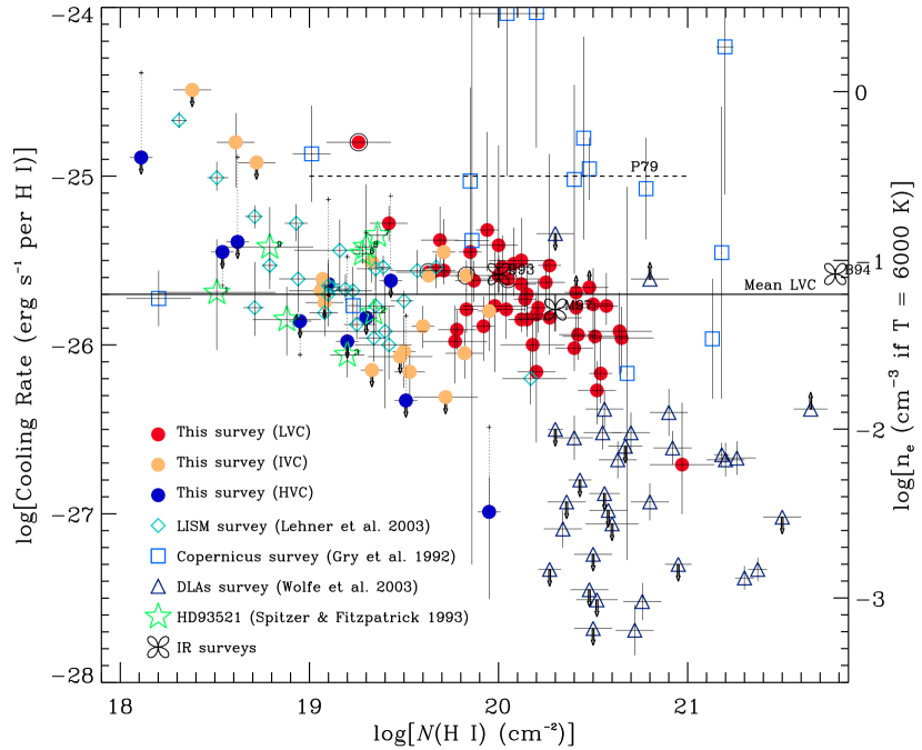
Figure 9: The logarithm of the cooling rate per H atom (left $y$-axis) is plotted against the H i column density from our survey for low-, intermediate-, and high-velocity clouds. These results are compared to other Galactic FUV and high-latitude FIR datasets, and the damped Ly $\alpha$ surveys. The different results are coded with the symbols given in the legend. The cooling rates per H atom of the values surrounded by an open circle are uncertain. For the high-latitude FIR, the results are from Bock et al. (1993, B93, for $\log N($H i$)>20.00$ dex); Bennet et al. (1994, B94, for $\log N($H i$)<21.78$ dex); Matsuhara et al. (1997, M97, for $\log N($H i$)<20.30$ dex). The horizontal dashed line shows the mean cooling rate per nucleon of the study by Pottasch, Wesselius, & van Duinen (1979) (their H i column densities lie between about 19 and 21 dex). The mean value of the cooling rates per H atom observed for LVCs in our sample is indicated by the solid horizontal line. Note that for the Gry, Lequeux, & Boulanger (1992) survey, the cooling rate is actually in erg s^-1  per nucleon (and note also that not all their H i column densities have errors). The logarithm of the electron density from our survey (assuming a temperature of 6000 K and solar abundances) is shown on the right $y$-axis. The dotted lines joining some of the data points correspond to the correction to $n_{e}$ for the metallicity and dust (see § 7.3 for more details).

The C II cooling rates were computed with Eqs. 4 and 5 and are summarized in Table 4 in erg s^-1  per H atom (column 2 using the H I emission measurement) and in erg s^-1  per nucleon (in column 3 where S II was used as a proxy for H, respectively). Note that Table 4 differs from Table 3 in the sense that types of clouds (LVCs, IVCs, or HVCs) are grouped together. The cooling rates in erg s^-1  per H atom are also shown graphically in Fig. 9 against the H I column density. This figure not only shows possible systematic trends of the observed cooling rates with the amount of H I, but also compares our results with others obtained from local FUV observations and IR observations at high Galactic latitudes and also in damped Ly $\alpha$ systems toward QSOs. Those other observations are discussed below and are summarized in Table 5, along with our observations.

6.1 Low-Velocity Clouds

6.1.1 Mean and Range of the Cooling Rates

The C II cooling rates for the LVCs span about an order of magnitude lying between $-26.3$ and $-25.3$ dex (see Table 4, Figs. 9 and 11), if we exclude Mrk 1095 ($\log l_{c}=-26.70$ dex) and limits or uncertain values (see below for more details on these sightlines). The mean cooling rate per H atom is $\log[(\Sigma_{1}^{N}l_{c})/N]=\log\langle l_{c}\rangle=-25.70\pm\,^{0.19}_{0.35}$ dex. The mean cooling rate per nucleon, using S II, is $\log\langle L_{c}\rangle=-25.65\pm\,^{0.11}_{0.15}$ dex. The errors given here are the deviation around the mean. The typical $1\sigma$ errors from the measurements are small enough to imply that the observed dispersion is a real change of the cooling rate from sightline to sightline. Note that the mean value was derived excluding the two sightlines where LVC and IVC components are blended (see Table 4). Note also that the sample to obtain $\langle L_{c}\rangle$ is much smaller than the sample to obtain $\langle l_{c}\rangle$ and is biased toward H I column densities larger than 10²⁰ cm^-2 (see Fig. 8), where ionization effects are less likely. Using the same sample to calculate the cooling rate per H atom and per nucleon, $\log\langle l_{c}\rangle=-25.61\pm\,^{0.17}_{0.27}$ dex. In Fig. 10, we compare the cooling rates per H atom and per nucleon. The straight line is a 1:1 relationship. There is a scatter of about $\pm 0.1$ dex around this line, except for 4 cases (where $\log N($H I$)\leq 20$ dex) that depart by more than $+0.1$ dex.

6.1.2 Dispersion of the Cooling Rates

Fig. 11 shows the LVC cooling rate against the H I column density for $\log N($H I$)>19.5$ dex. The solid line shows the mean cooling rate, with the dotted lines giving the $1\sigma$ dispersion around the mean. Two features are apparent from this figure: (1) a large scatter of $l_{c}$ of about 0.5 dex (a factor $\sim$3 change from sightline to sightline) at any given $N($H I); (2) a decrease of $l_{c}$ with increasing $N($H I).

The decrease of the cooling rate per H atom with increasing $N($H I) can be understood as an ionization effect. In § 7.1, we show that a substantial fraction of the observed C II* may come from the ionized region of the cloud, where more electrons are present. In § 2 we saw that collisional excitation of C II with electrons is far more efficient than with hydrogen atoms in the diffuse warm gas. So, at low H I column density (less than a few $10^{19}$ cm^-2), this effect is very apparent because the fraction of photoionized gas is significant ($\gtrsim 90$% if $\log N_{e}\sim 19.9$ dex, see § 5.1). For example, for $\log N($H I$)<19.5$ dex, the largest deviation from the mean cooling rate is observed, toward HE 1228+0131 in component 4 at $+27$ ${\rm km\,s}^{-1}$, where $\log l_{c}\approx-24.80$ dex, nearly 8 times higher than the mean value. The cooling rate derived with S II implies a lower value, $-25.30$ dex, still a factor $\sim 3$ times higher than the mean value. The ratio [S II/H I$]\sim+0.5$ dex also implies a substantial fraction of ionized gas along this sightline. A similar high value for the cooling rate is also found toward 3C 273, only 0$\fdg$83 away from HE 1228+0131, for the $+25$ ${\rm km\,s}^{-1}$ component number 4. At higher H I column densities, the fraction of ionized gas must diminish to about 10–50% (assuming $\log N_{e}\sim 19.9$ dex). In Fig. 11, the sightline for which the cooling rate departs most from the mean is Mrk 1095. It has the lowest cooling rate, a factor 10 smaller than $\langle l_{c}\rangle$ for the largest H I column density in our sample (20.97 dex). If $\log N_{e}\sim 19.9$ dex, the gas along this sightline is almost entirely neutral. The depletion of Fe for this sightline informs us that the gas is mostly warm. Models of multi-phase gas predict very low C II cooling rates for the WNM (a factor $\sim 10$ times smaller than the cooling rates in the WIM or the CNM, Wolfire et al. 1995) roughly on the order of the cooling rate measured toward Mrk 1095.

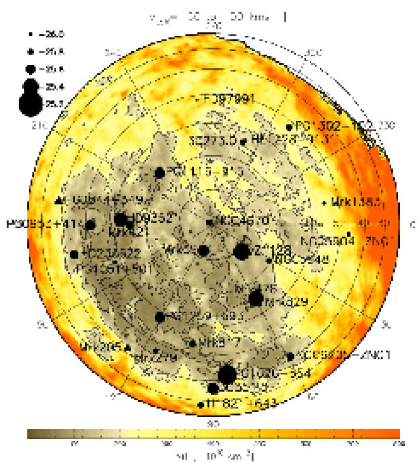
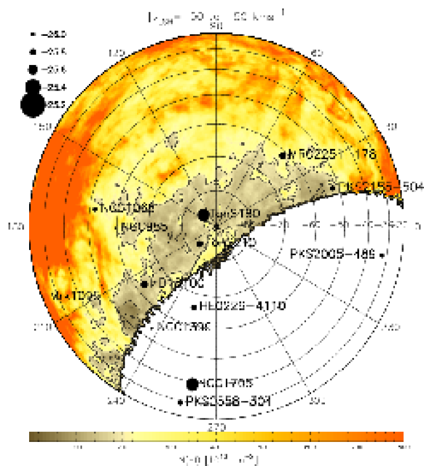
Figure 12: H i contour map of the northern galactic sky (left diagram) and southern galactic sky (right diagram) for LSR velocities between $-50$ and $+50$ ${\rm km\,s}^{-1}$. The LVC cooling rates per H atom, $l_{c}$, for each survey object are displayed with the filled circles. The circle size is proportional to $\log l_{c}$ according to the legend. A lower limit for PG 0844+349 is marked with a filled triangle. The H i contour levels are at 5, 20, 50, 100, $200\times 10^{18}$ cm^-2.

In Fig. 12, we show the cooling rates projected on the Galactic northern (left hand-side) and southern (right hand-side) sky, where the H I contours show the column density for gas with $\mid\!v_{\rm LSR}\!\mid\leq 50$ ${\rm km\,s}^{-1}$. This figure confirms the above discussion: in regions with higher H I columns, the C II* cooling rate in LVCs is lower in both the south and north Galactic sky and vice-versa. There does not appear to be a latitude or longitude dependence or a north-south asymmetry within the errors. We also did not find any relation between the cooling rate and the distance for the stellar sightlines given in Table 2, suggesting that the bulk of the observed gas is at $z<800$ pc (smallest $z$-height in our sample). We note, however, a decrease in the cooling rates with $z$-height when the LVC, IVC, and HVC are considered together. For IV Arch at $z\sim 1$ kpc we find that on average the cooling is a factor 2 lower (see § 6.2) and for Complex C, at $z>6$ kpc it is 20 times lower (see § 6.3).

The observed dispersion in the cooling rates in the LVCs certainly does not have a single explanation. The change in the ionized fraction explains why the cooling rates decrease at higher H I columns. In the WNM, a change in the temperature of the gas can affect which cooling process dominates. For example, Wolfire et al. (2003) show that for $500\lesssim T\lesssim 8000$ K the cooling due to [O I] 63 $\micron$ becomes more important than [C II] 158 $\micron$, and collisional excitation of Ly$\alpha$ dominates the cooling if $T\gtrsim 8000$ K. Also, variations in the heating that balances the cooling are expected in gas heating models (Reynolds, Haffner, & Tufte, 1999; Wolfire et al., 2003). To explain the emissivity of C II in the WNM, photoelectric heating from small grains and PAHs appears to be the dominant heating process (e.g., Wolfire et al., 2003). So, the dust-to-gas fraction may also vary, although there is no direct evidence for this variation from our observations. The cooling rate per H atom does not increase with smaller values of [Fe II/H I], but note that the depletion of elements such as Fe does not really determine if the total dust-to-gas fraction is varying, since dust and PAHs are believed to be mostly composed of C and Si (Draine, 2003). Pure photoionization models of the WIM have a heating rate per unit volume about $\sim 10^{-24}\times n_{e}^{2}$, so photoionization of H can provide only part of the heating of the diffuse gas because $n_{e}\simeq 0.08$ cm^-3 (Reynolds & Cox, 1992; Reynolds, Haffner, & Tufte, 1999; Slavin, McKee, & Hollenbach, 2000). Photoelectric grain heating of the WIM can provide a supplemental heating mechanism (Reynolds & Cox, 1992; Draine, 1978). However, other sources are possible, such as the dissipation of interstellar plasma turbulence that may even dominate over photoionization in regions where $n_{e}<0.1$ cm^-3, because the heating rate per unit volume is in that case about $\sim 10^{-25}\times n_{e}$ (Minter & Spangler, 1997; Reynolds, Haffner, & Tufte, 1999). Other heating processes in the WIM may include magnetic-reconnection (e.g., Raymond, 1992), or coulomb collisions by cosmic rays (e.g., Skibo, Ramaty, & Purcell, 1996), although it is not clear if they are a significant source of heating.

6.2 Intermediate-Velocity Clouds

The main IVC investigated is the IV Arch. Table 4 presents the cooling rate for the individual sightlines through this complex. The mean cooling rate per nucleon in the IV Arch using S II, $\log\langle L_{c}\rangle=-25.98\pm\,^{0.09}_{0.12}$ dex. The errors given here are the deviation around the mean. The mean cooling rate per H atom appears to be $\log\langle l_{c}\rangle=-25.76\pm\,^{0.22}_{0.46}$ dex. But much higher values are found toward Mrk 205 ($-25.45$) and PG 0953+414 ($-25.51$). However, the IV Arch is substantially ionized toward these two sightlines and indeed, if those sightlines are not included or if the ionization is corrected for, the mean cooling rate per H atom would be $\log\langle l_{c}\rangle=-25.98\pm\,^{0.14}_{0.20}$ dex, in agreement with the mean derived using S II. The mean cooling rate of $-25.98$ dex in the IV Arch is about two times smaller than the mean cooling rate of the LVCs.

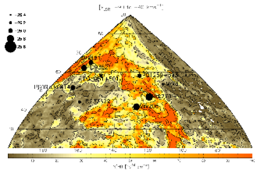
Figure 15: H i contour map of the IV Arch for LSR velocities between $-90$ and $-40$ ${\rm km\,s}^{-1}$, where the colors denote the H i column density. Galactic longitude and latitude are displayed on the figure. The logarithms of the cooling rates per H atom derived from the C ii* UV observations are shown for each extragalactic or stellar direction as filled circles for actual measurements, with circle size proportional to $\log l_{c}$ (see the legend). Mrk 59 and NGC 4151 are not shown because the IVC and LVC absorption are blended. The very uncertain measurement for NGC 4051 is also omitted. A $3\sigma$ upper limit for Mrk 817 is marked with a filled triangle. The H i contour levels are at 5, 20, 50, 100, $200\times 10^{18}$ cm^-2.

In Fig. 14, we show the cooling rate against the H I column density for the IV Arch components. There may be an increase of the cooling rate with $N($H I), (but the number of data points is small) if the low limit toward PG 1051+501 is not taken into account. The stellar continuum of PG 1051+501 is uncertain, producing uncertain results. In Fig. 15, the cooling rates of the individual sightlines are overplotted on an H I contour map, showing again that the higher values of the cooling rates are in the higher H I column density regions.

The strength of the FUV radiation field that heats the gas may be lower in the IV Arch (resulting in a weaker cooling in the IV Arch) because the IVC is more distant than the LVCs. The slight increase of the cooling rate with increasing $N($H I) suggests that the emissivity of C II is higher in the denser and neutral regions of the IV Arch. This behavior contrasts with the decrease of $l_{c}$ with increasing $N($H I) observed in the LVCs, but this effect could just be because of the small number of sightlines.

In the IV Spur (PG 1116+215, S1 component), about 20% of the gas is in ionized form. The cooling rate per nucleon is $-25.65$ dex (mean of the cooling using S II). The Spur region is believed to be an extension of the IV Arch. Including $\log l_{c}=-25.65$ dex and $\log N($H I$)=19.83$ dex with the data points in Fig. 14 would strengthen the evidence for an increase of the cooling rate with increasing $N($H I) in the IV Arch.

The IVC at positive velocities toward PKS 2005–489 is only detected in the metal absorption lines. Therefore, we can only make a rough estimate of the cooling rate using P II, assuming no depletion affects P in this IVC. The cooling rate per nucleon inferred from P II is $-25.28$ dex, the highest cooling rate in our sample (including the LVCs) for an H column density of $\sim 19.80$ dex (also inferred from P II).

The largest deviation from the mean cooling rate of the LVCs is observed in IVC component 2 at $+40$ ${\rm km\,s}^{-1}$ toward Ton S180, where $\log l_{c}\simeq-24.80$ dex, nearly 8 times higher than $\langle l_{c}\rangle$ of the LVCs. The H I column density toward Ton S180 (component 2) is small, 18.61 dex, and for such small column density, there must be an appreciable amount of H II along the sightline. We do not have information from the other ions for this component to better characterize its properties. Lehner et al. (2003) find higher cooling rates per H atom in the LISM at similar H I column densities (see Fig. 9). The presence of a substantial amount of H II and C II* in the ionized gas is the most likely explanation (Lehner et al., 2003).

Only $3\sigma$ upper limits were derived for IVC-K, IVC-gp, and the IVC toward NGC 1068. The high limits toward MRC 2251–178 (IVC-gp) and Mrk 478 (IVC-K) are not really stringent because of a combination of low S/N and low H I column density. The limit toward NGC 1068 is within the observed range of cooling rates.

6.3 High-Velocity Clouds

We find a cooling rate of about $-26.99$ dex in Complex C toward PG 1259+593 (per H atom or per nucleon, see Table 4), which is 20 times smaller than the mean cooling rate of the LVCs. Only $3\sigma$ upper limits were derived for the other sightlines through the Complex (see Table 4). Toward Mrk 817, the upper limit on the cooling ratio is at least 4 times smaller than the Galactic LVC mean value, suggesting that the cooling is generally weak in Complex C. The other sightlines do not provide stringent limits because the S/N ratio is not high enough.

Complex C has a low metallicity (see § 5.3). If C follows a similar abundance pattern to that of Fe, S, and Si ([C/Si$]\sim-0.1$ dex, Fox et al. 2004), it would also be underabundant with respect to the solar abundance by about a factor 5–6. Yet, the cooling rate toward PG 1259+593 is more than 20 times smaller than the mean value observed in Galactic Halo gas. A lower C abundance can only explain in part why the cooling rate is so low in Complex C. Heating and cooling from dust in Complex C cannot be important because there is no evidence of dust. The weak emissivity of C II in Complex C with respect to the LVCs and IVCs could be a signature of a weaker FUV field. Or it could be that the cooling from [C II] emission is a not major cooling process because of a mixture of lower metallicity, warmer gas, and more neutral gas than sampled in the LVCs. In the WNM, Wolfire et al. (2003) show that for $500\lesssim T\lesssim 8000$ K the cooling due to [O I] at 63 $\micron$ becomes more important, and collisional excitation of Ly$\alpha$ (independent of the metallicity) dominates the cooling if $T\gtrsim 8000$ K. In the pure WNM, the cooling from [C II] emission is estimated to be a factor $\sim$10 lower than in the WIM (Wolfire et al., 1995). But while the metallicity is indeed low in Complex C, there is no evidence that it has warmer or more neutral gas than the LVCs or IVCs. The FHWM of the H I emission profile implies a temperature $T\lesssim 8800$ K. Complex C is also known to contain ionized gas, as revealed through H$\alpha$ emission (Tufte, Reynolds, & Haffner, 1998; Wakker et al., 1999). Wakker et al. (1999) derived a temperature in Complex C of $T=7300\pm 900\pm^{1500}_{1000}$ K toward Mrk 290.

We explore another kind of HVC, the Outer Spiral Arm region of the Galaxy. We have only a $3\sigma$ upper limit for the cooling rate per H atom: $-25.86$ dex (see Table 4, the H 1821+643 sightline). This limit is below the mean value observed in Galactic Halo gas, and in particular for similar or lower H I column density observed in the local gas (Gry, Lequeux, & Boulanger, 1992; Lehner et al., 2003, see Fig. 9). We note that our $3\sigma$ upper limits are estimated without taking into account the error on the H I column density. However, toward H 1821+643 in particular, the $1\sigma$ error is small, only $\pm 0.06$ dex. Hence, the derived upper limits are lower than the cooling rate for lower-velocity components in the Galaxy.

While Complex C and the Outer Arm (OA) are unrelated HVCs, they both contain little or no dust, have ionized gas kinematically related to the neutral gas, and possibly trace exclusively warm gas ($T\sim 7000-8000$ K). They are also distant. Complex C is believed to be extragalactic and at least 6 kpc away from the Milky Way disk. The OA HVC could be at a galactocentric distance of $\sim$24 kpc. This may imply that the FUV radiation field in these HVCs is substantially weaker, and hence other sources of heating from EUV and X-rays may be important. A possible signature of EUV and (soft) X-ray radiation is O VI absorption detected toward these sightlines at similar velocities as the low ionization species. In particular, Fox et al. (2004) showed that the high ions in Complex C toward PG 1259+593 are probably produced in an interface between cool/warm gas and a surrounding hot medium. The interface is a possible source of EUV radiation and the surrounding hot gas is a source of X-ray radiation.

Toward Mrk 205, the very high-velocity cloud WW84 also gives a $3\sigma$ upper limit 1.5 times smaller than the mean value observed in our Galaxy.

6.4 Comparison with Other (More Local) UV Observations

Pottasch, Wesselius, & van Duinen (1979) measured the C II cooling rates per nucleon for the interstellar gas outside dense H II regions toward 9 early-type stars. Their study was based on Copernicus and IUE observations. They found that the cooling rates did not appear to vary substantially from one cloud to another, although they did not produce any error estimates. They found a mean cooling rate around $-25$ dex (per nucleon). Their mean is indicated by horizontal dashed line in Fig. 9. It is substantially higher than most of our measurements and the results of other studies at similar H I column densities. Their cooling rates may be biased toward high values since the FUV radiation fields appear to be greater toward at least some of their sightlines than the interstellar average (Wolfire et al., 1995).

Gry, Lequeux, & Boulanger (1992) extended the Pottasch, Wesselius, & van Duinen (1979) study by gathering Copernicus observations to measure C II* column densities toward 20 stars that are situated at distances of a few hundred pc to 1.4 kpc. They found a dispersion larger than the errors in the cooling rates from direction to direction, with a mean value of $-25.46\pm 0.41$ dex (per nucleon), smaller by 0.46 dex than the value of Pottasch, Wesselius, & van Duinen (1979), but higher by 0.24 dex than along the Galactic halo sightlines presented in this study (see the summary Table 5). The magnitude of the scatter of the cooling rates is larger than the one observed in our survey, but note that several of their measurements have $1\sigma$ error larger than $>\pm 0.7$ dex (see Fig. 9). Because their background FUV sources are early-type stars, Gry, Lequeux, & Boulanger (1992) expected that some of the C II* cooling takes place in the H II regions which surround the stars. This would explain the higher mean cooling rate in their survey. Cold gas is also more likely to be present along their sightlines.

Lehner et al. (2003) derived the cooling rates in the LISM toward 31 white dwarf stars located less than 200 pc from the sun. If we exclude two of their sightlines for which substantial ionization corrections are needed, their mean cooling rate per H atom is $l_{c}=-25.63\pm\,^{0.18}_{0.33}$ dex. Their mean and dispersion of the cooling rate in the LISM are very similar to what we find for the Galactic Halo interstellar clouds (see Table 5 and Fig. 9), suggesting a similarity of the physical properties of the LISM and the Galactic Halo gas.

6.5 Comparison with Galactic Halo IR Observations

Another method to obtain the C II cooling rate per H atom is from direct measurements of the [C II] 157.7 $\micron$ line via IR observations. Bock et al. (1993) measured the [C II] emission line toward three directions between $l=135\arcdeg-150\arcdeg$ and $b=33\arcdeg-50\arcdeg$. The emission of [C II] is observed in all directions, it correlates well with $N($H I). They found a cooling rate that spans values from $l_{c}=-25.92$ to $-25.49$ dex (for $N($H I$)>10^{20}$ cm^-2), with a best-fit value of$-25.58\pm 0.10$ dex, excluding the cases with low line-to-continuum ratios and the lines of sight with CO emission. Matsuhara et al. (1997), using the same data but concentrating on high Galactic latitude molecular clouds, found $l_{c}=-25.80\pm 0.11$ dex for $N($H I$)<2\times 10^{20}$ cm^-2. At high galactic latitude and on nearly the full Galactic sky with two instruments (FIRAS and DIRBE) onboard of the Cosmic Background Explorer (COBE) Bennett et al. (1994) found a best-fit value of $l_{c}=-25.57\pm 0.03$ dex, while Caux & Gry (1997) found $l_{c}=-25.48\pm 0.04$ dex with the Infrared Space Observatory (ISO). Note that the errors reported in the FIR studies are the errors on the fit between the [C II] 157.7 $\micron$ intensity and the H I column density, and not the dispersion of the measurements.

Within the IR measurements there is some scatter between the different best-fit values of $l_{c}$. But the range of cooling rate values and the best-fit values reported in the IR studies at high galactic latitudes are in good agreement with the mean cooling rate and dispersion derived in our survey for the Galactic halo gas (LVCs), which is important in view of the fact that these two methods are completely different. Bennett et al. (1994) argued that this emission arises almost entirely from cold regions. Makiuti et al. (2002) using the Far-Infrared Line Mapper (FILM) aboard of the Infrared Telescope in Space (IRTS) recently argued that [C II] emission must mostly come from the WIM at high Galactic latitudes. Our analysis also shows that at $\mid\!b\!\mid\gtrsim 30\arcdeg$ a large fraction of [C II] comes from the WIM (see § 7.1). We also note that Heiles (1994) shows that the ionized medium could explain the bulk of [C II] in the inner Galaxy.

7 Other Implications of the C II* Absorption

7.1 The Origin of C ii* at High Galactic Latitude

The column density of C II* in the WIM can be estimated in the following way (R. J. Reynolds 2004, private communication): In § 2 we discuss that in the WIM and WNM conditions, Eq. 1 can be simplified, and so can be written in the WIM as:

$$n({\rm C^{+*}})A_{21}=n({\rm C^{+}})n_{e}\gamma_{12}(e)$$ (6)

We can integrate Eq. 6 over the line of sight as follows:

$$\int\alpha{({\rm H\alpha})}A_{21}n({\rm C^{+*}}){\rm d}s=10^{6}\int\frac{n({\rm C^{+}})}{n({\rm C})}\frac{n({\rm C})}{n({\rm H})}\frac{n({\rm H})}{n({\rm H^{+}})}\gamma_{12}(e)\frac{\alpha{({\rm H\alpha})}}{10^{6}}n_{e}n({\rm H^{+}}){\rm d}s\,,$$

or, assuming that the fractions of C II, C, and H II are constant (see below),

$$\alpha{({\rm H\alpha})}A_{21}N_{\rm WIM}({\rm C^{+*}})=10^{6}\frac{n({\rm C^{+}})}{n({\rm C})}\frac{n({\rm C})}{n({\rm H})}\frac{n({\rm H})}{n({\rm H^{+}})}\gamma_{12}(e)I[{\rm H\alpha}]\,,$$

where

$$I[{\rm H\alpha}]=\int\frac{\alpha{({\rm H\alpha})}}{10^{6}}n_{e}n({\rm H^{+}}){\rm d}s$$

is the velocity-integrated surface brightness of diffuse H$\alpha$ emission in Rayleigh ($1{\rm R}\tbond 10^{6}/4\pi$ photons cm^-2 s^-1 sr^-1). $\alpha{({\rm H\alpha})}=1.17\times 10^{13}$ cm³ s^-1 (Martin, 1988; Osterbrock, 1989) is the recombination coefficient of H$\alpha$ at $T=10^{4}$ K, and all the other symbols are defined in § 2. We assume the temperature in the WIM $T=10^{4}$ K based on Reynolds (1993) study. Assuming that C II is the dominant ion in the WIM (Sembach et al. 2000 modeled the WIM and showed that C III is negligible with respect to C II, and see also Reynolds 1992), $n({\rm C^{+}})/n({\rm C})\simeq 1$. Assuming that the gas-phase abundance of C is the same in the diffuse CNM, WNM and the WIM, $n({\rm C})/n({\rm H})\simeq 1.42\times 10^{-4}$ (Sofia et al., 1997). Finally, in the WIM, $n({\rm H})/n({\rm H^{+}})\simeq 1.1$ (Reynolds, 1989). Then the column density of C II* in the WIM is simply given by,

$$N_{\rm WIM}({\rm C^{+*}})=7.23\times 10^{13}I[{\rm H}\alpha]\,\,{\rm cm}^{-2}\,.$$ (7)

The $I[{\rm H\alpha}]$ intensity was measured by the Wisconsin H$\alpha$ mapper (WHAM) (Haffner et al., 2003) over a $1\arcdeg$ diameter field of view that contains the background object, but not centered on the object. In Table 6, we list the sightlines for which there is a $I[{\rm H\alpha}]$ measurement, where $\Delta\theta$ is the distance in degrees to the nearest H$\alpha$ survey gridpoint. For HD 93531, we list the results from the WHAM survey as well as the direct pointing of WHAM on that object, in which the LVC and IVC components were separated (Hausen et al., 2002). In this table, $N_{\rm obs}($C II*) is the observed C II* column density that includes the LVC and the IVC components, because $I[{\rm H\alpha}]$ is integrated over $\sim\pm 100$ ${\rm km\,s}^{-1}$ in the WHAM survey. We did not include the measures for which $N_{\rm obs}($C II*) is a lower limit or uncertain. We also did not include the value of $I[{\rm H\alpha}]=18.6$ R toward Mrk 1095 because such a high value is certainly contaminated by a dense H II region not associated with the diffuse WIM and WNM (this line of sight lies the closest to the galactic plane, at $b\simeq-21\arcdeg$). In Table 6 we tabulate the estimated values of $N_{\rm WIM}($C II*) and $N_{\rm WIM}($C II*$)/N_{\rm obs}($C II*). We show in Fig. 13 $N_{\rm WIM}($C II*) against $N_{\rm obs}($C II*).

The fraction $N_{\rm WIM}($C II*$)/N_{\rm obs}($C II*) varies significantly from sightline to sightline between 0.1 to 1. The mean and median values of $N_{\rm WIM}($C II*$)/N_{\rm obs}($C II*) both are 0.5, with a dispersion of 0.2. This calculation contains uncertainties. The gas-phase abundance of C in the WIM may be different than in the diffuse CNM. If the abundance of C in the WIM is solar, this would increase $N_{\rm WIM}($C II*) by a factor 1.73, and in that case the mean of $N_{\rm WIM}($C II*$)/N_{\rm obs}($C II*) would be 0.8. If the temperature of the WIM is 8000 K instead of $10^{4}$ K, $N_{\rm WIM}($C II*) would increase by about 10%. However, the fractions $n({\rm C^{+}})/n({\rm C})\simeq 1$ and $n({\rm H})/n({\rm H^{+}})\simeq 1.1$ should not change by much more than 5–10% in the WIM (Reynolds, 1989; Sembach et al., 2000). Hence, the uncertainties of the different factors used to estimate $N_{\rm WIM}($C II*) show that the fraction of C II* in the WIM is at least 0.5.

Another uncertainty is that the gas sampled by WHAM and the FUV measures may not be the same because of the 1° field of view of WHAM compared to the very small angles subtended by the AGNs or stars. The effect of this uncertainty can not be easily quantified. Toward HD 93521, $N_{\rm WIM}($C II*) does not change much between a direct pointing on that object and the 0$\fdg$41 distant pointing, at least for the LVC component. On the other hand, toward vZ 1128 we know that the fraction of ionized hydrogen is 46% and the ionized and neutral phases are kinematically related (Howk, Sembach, & Savage, 2004), so it is surprising that only 13% of $N_{\rm obs}($C II*) comes from the WIM based on the H$\alpha$ estimates. We note that for another pointing 0$\fdg$6 away from vZ 1128, $I[{\rm H\alpha}]$ is 2.8 times the value of $I[{\rm H\alpha}]$ given in Table 6. In contrast, toward both NGC 5904-ZNG1 and NGC 6205-ZNG1, where 20% and 40% of hydrogen is ionized (see § 5.1), at least 50% of $N_{\rm obs}($C II*) is from the WIM. $I[{\rm H\alpha}]$ should, however, not be systematically high or low, so that if the individual sightline may suffer from some uncertainty because of the 1° field of view of WHAM, the average value of $N_{\rm WIM}($C II*$)/N_{\rm obs}($C II*) should not be affected by the irregular distribution of the gas.

7.2 The Integrated Galactic C II Radiative Cooling Rate

Since we know the C II radiative cooling rate per H atom and per nucleon toward many sightlines in the Milky Way, we can make a rough estimate of the total C II cooling rate for the diffuse gas in the entire Galaxy. If we assume an exponential disk, the total number of warm H atoms in the Galaxy can be written:

$$N({\rm atoms})=\int_{0}^{2\pi}\int_{-\infty}^{+\infty}\int_{0}^{R_{\rm max}}n(0)\,e^{(-z/h)}\,e^{(-R/H)}\,R\,dR\,dz\,d\phi\,,$$ (8)

where $H$ and $h$ are the scale lengths and scale heights, respectively, $R_{\rm max}\simeq 25$ kpc (Kulkarni, Heiles, & Blitz, 1982; Diplas & Savage, 1991), and $n(0)(=n(R_{\odot})e^{(R_{\odot}/H)})$ is the mid-plane density at the galactic center. Assuming that $h$ is independent of $R$, the total number of warm H atoms in the Milky Way is then

$$N({\rm atoms}) = 2\pi e^{(R_{\odot}/H)}H^{2}N_{\perp}\int_{0}^{R_{\rm max}}e^{(-R/H)}(R/H){\rm d}(R/H)\,$$ (9)

$$\simeq 2\pi e^{(R_{\odot}/H)}H^{2}N_{\perp}\,,$$

where $H\simeq 3$ kpc (Diplas & Savage, 1991) and $R_{\odot}=8.5$ kpc. We estimated the total average perpendicular column density of neutral hydrogen for the WNM measured at the position of the Sun, $R_{\odot}$, from the Leiden/Dwingeloo H I survey (Hartmann & Burton, 1997), $N_{\perp}($H I$)=2\times(2\times 10^{20})$ cm^-2. Taking into account that the total average perpendicular column density for the WIM at $R_{\odot}$ is $N_{\perp}($H II$)=2\times(7.1\times 10^{19})$ cm^-2 (Reynolds, 1993), the total perpendicular H column density at $R_{\odot}$ is $5.4\times 10^{20}$ cm^-2. So, with the mean cooling rate of the LVCs, the total luminosity associated with the C II cooling in the Galaxy from the WNM and WIM (where we assume that the local conditions apply to the entire Galaxy) is $L\simeq 9.9\times 10^{40}$ erg s^-1 or $L\simeq 2.6\times 10^{7}$ L_⊙. Wright et al. (1991) found a higher value with COBE, $L\simeq 5.0\times 10^{7}$ L_⊙. Shibai et al. (1991) found a similar value ($L\simeq 2.7\times 10^{7}$ L_⊙), using a balloon experiment along the galactic plane for $21\arcdeg\leq l\leq 51\arcdeg$.

7.3 Electron Density

Using Eq. 3 (at $T=6000$ K, $n_{e}\simeq 15.29N({\rm C}^{+*})/N({\rm C}^{+})$ cm^-3) our data also allow estimates of the electron density in the gas. The C II $\lambda$$\lambda$1036, 1334 absorption lines are, however, extremely strong, and the C II column density can not be estimated reliably. C is lightly depleted into dust grains ($-0.2$ dex, Cardelli et al. 1996; Sofia et al. 1997; Jenkins 2003). Therefore we can use S II as a proxy for C II. Only a small percentage, if any, of S is incorporated into dust grains, but C is lightly depleted by $-0.2$ dex, which needs to be taken into account. The first ionization stage of all these species is also the dominant one in warm gas. So, we can assume $N($C II*$)/N($C II$)\approx 10^{0.2}N($C II*$)/N($S II$)\times({\rm S}/{\rm C})_{\odot}$, where the solar ratio $\log({\rm S}/{\rm C})_{\odot}=-1.06$ dex (Grevesse & Sauval, 1998; Allende Prieto, Lambert, & Asplund, 2002). If C II is mostly in H I regions, we can also use our H I measurement, the Allende Prieto, Lambert, & Asplund (2002) C solar abundance ($\log({\rm C}/{\rm H})_{\odot}=-3.61$) and a depletion of $-0.2$ dex of C to estimate $n_{e}$. Note that we did not make any correction for depletion effects in the HVCs. For Complex C and WW84 we have corrected for the metallicity when H I is used as a proxy for C II.

The electron densities are summarized in Table 4 and displayed for $n_{e}($H I) in Fig. 9 against $N($H I), where a temperature of the gas of 6000 K was assumed. Because $n_{e}\propto l_{c}$, the main discussion in § 6 about variations in the cooling rates and the origin of C II* directly applies to $n_{e}$. Here, we summarize the mean value of $n_{e}$ and dispersion for the different type of clouds investigated.

The LVCs: We find a mean value of the electron density (using H I or S II) of $\langle n_{e}\rangle=0.08\pm 0.04$ cm^-3 when $T=6000$ K, and a range of values, $0.02\lesssim n_{e}\lesssim 0.17$ cm^-3. The only value departing from this range is $n_{e}\simeq 0.006$ cm^-3 toward Mrk 1095, confirming that this sightline is predominantly neutral. In the LISM and in the high galactic latitude diffuse clouds from other FUV measurements, the range of measured electron densities was found to be $0.01\lesssim n_{e}\lesssim 0.15$ cm^-3 for temperatures of about 6000–7000 K, with an average value of about 0.07 cm^-3 (e.g., Savage et al., 1993; Spitzer & Fitzpatrick, 1993, 1995; Savage & Sembach, 1996a; Gry & Jenkins, 2001; Lehner et al., 2003). The mean, dispersion, and range are thus similar to those found in previous FUV studies, but now with a better statistic at high galactic latitudes. The electron density has also been inferred from a comparison of the H$\alpha$ emission with the dispersion measure for pulsars in globular clusters. Using this method, Reynolds (1991) found also an average electron density of 0.08 cm^-3 toward four high Galactic latitude globular clusters (this work includes two directions in our sample, NGC 5904 and NGC 6205).

The IVCs: In the IV Arch, we have $\langle n_{e}\rangle\simeq 0.03\pm 0.01$ cm^-3 when $T=6000$ K, and a range of values of $0.01\lesssim n_{e}\lesssim 0.05$ cm^-3. The other IVCs have similar electron density (see Table 4), except toward Ton S180 ($n_{e}\simeq 0.54$ cm^-3) but for which a substantial ionization correction is necessary because $n_{e}$ was derived using the H I column density. For the IVC toward HD 93521, Spitzer & Fitzpatrick (1993) also reported a similar electron density.

The HVCs: Only one tentative measurement is derived, toward PG 1259+593, giving $n_{e}\sim 0.01$ cm^-3. The $3\sigma$ upper limits toward the other targets are in the range observed for the lower velocity clouds.

7.4 Damped Ly $\alpha$ Systems

In Fig. 9 we compare our results to the recent survey of C II cooling rates in the damped Ly $\alpha$ systems (DLAs) reported by Wolfe, Prochaska, & Gawiser (2003). The mean cooling rate and dispersion around the mean are summarized in Table 5. A comparison of the means reveals that $\log\langle l_{c}\rangle$ in the DLAs is $\sim$1 dex less than value of $\log\langle l_{c}\rangle$ of the LVCs in the Galactic Halo. For $\log N($H I$)\gtrsim 20.5$ dex, the difference with the Galactic Halo sightlines is smaller. The dispersions of the cooling rates are similar in both samples. We discussed that the variation in the Milky Way cooling rate has certainly several origins, including changes in the ionization fraction, in the dust fraction, and in the physical conditions. In the DLAs, Wolfe, Prochaska, & Gawiser (2003) proposed that the variation is due to different star-formation rates (SFRs). In order to derive the SFR in the DLAs, the models of Wolfe, Prochaska, & Gawiser (2003) assume that the reservoir of C II* in the DLAs gas comes from the CNM. Recently, Howk, Wolfe, & Prochaska (2004) directly show that cold gas is likely the dominant contributor to C II* for one DLA of their sample. However, while Vladilo et al. (2001) (using the ratio of Al III/Al II) showed that the ionization correction for elemental abundance analysis may be unimportant, the ratio of Al III/Al II in most DLAs implies nonetheless a significant fraction of ionized gas in the DLAs, similar to that observed in the Milky Way. The presence of a WIM component in the DLAs could be an important contribution to the C II* in DLAs.

We also note the similarity of the measured cooling rates in Complex C and the DLAs. Complex C and DLAs both contain low-metallicity gas, but in Complex C there is no evidence for stars or dust. Also Wolfe, Prochaska, & Gawiser (2003) discussed that the main gas phase observed in the DLAs may be cold and neutral, while it is warm neutral and ionized in Complex C. Yet, the similar C II cooling rates in Complex C and DLAs suggest that some of the DLAs could be intergalactic clouds near galaxies like the gas in Complex C, rather than clouds in which stars are currently forming.

8 Summary

We present a survey of the [C II] $\lambda$157.7 $\micron$ radiative cooling rates from the C II* $\lambda$$\lambda$1037, 1335 absorption lines at galactic latitudes $\mid\!b\!\mid\gtrsim 30\arcdeg$ using FUSE and STIS observations. Our survey allows us to derive the C II cooling rates in the low-, intermediate-, and high-velocity clouds (LVCs, IVCs, HVCs). The main results are summarized in Tables 4 and 5, and in Fig. 9 and are discussed in § 6. Our main conclusions are summarized as follows:

1. For the LVCs, the logarithm of mean cooling rate in erg s^-1 per H atom is $-25.70^{+0.19}_{-0.36}$ dex ($1\sigma$ dispersion). With a smaller sample and a sample bias toward H I column densities larger than $10^{20}$ cm^-2, the cooling rate per nucleon is similar.

2. Our sightlines probe mostly warm clouds based on measures of the depletion of the Fe and P into dust. We are able to show that a substantial fraction of hydrogen is ionized (20–50%) toward a few of our sightlines, and argue that ionization is certainly important toward most of them. We find that a fraction of at least 0.5 of the observed C II* is produced in the WIM, using H$\alpha$ measurements in the direction of each object.

3. The observed dispersion in the cooling rates is larger than the individual measurement errors. The dispersion certainly arises from changes from sightline to sightline in the ionization fraction, dust-to-gas fraction, and physical conditions.

4. We derive a total Galactic C II luminosity for gas in the WNM and WIM of $L\sim 2.6\times 10^{7}$ L_⊙.

5. The mean and dispersion of the cooling rates of the LVCs observed at high Galactic latitudes in our survey are very similar to the cooling rates observed in the local ISM within 200 pc. The mean cooling rate is, however, a factor $\sim$2 lower than the FIR measurements at high latitudes, but compatible within our $1\sigma$ error.

6. The main IVC probed in our survey is the IV Arch located at $z\sim 1$ kpc. The logarithm of the mean cooling rate per nucleon is $-25.98$ dex with a dispersion of about $\pm\,^{0.14}_{0.20}$ dex. This value is 2 times smaller than the mean cooling of the LVCs, implying the cooling and hence the heating decrease at higher $z$.

7. Two IVCs toward PKS 2005–489 and Ton S180 with positive velocity for which the distance is unknown possess high cooling rates.

8. The observations of C II* yield estimates of $n_{e}$ in the absorbing gas. Assuming $T=6000$ K, for the LVCs, $\langle n_{e}\rangle=0.08\pm 0.04$ cm^-3 and for the IV Arch, $\langle n_{e}\rangle=0.03\pm 0.01$ cm^-3 ($1\sigma$ dispersion).

9. At large $z$ ($>6$ kpc), the C II cooling rate of the gas in Complex C is 20 times smaller than the average for the LVCs, implying that the heating and cooling processes are far weaker at large distance from the Milky Way disk.

10. The C II cooling rate found for high redshift DLAs by Wolfe, Prochaska, & Gawiser (2003) is $\sim$1 dex smaller than for the Galactic halo LVCs, but comparable to the cooling rate for the gas in Complex C.

11. Many of the DLAs have values of Al III/Al II similar to that found in the Milky Way, suggesting roughly similar amounts of ionized gas to neutral gas. Therefore, we would expect ionized gas in many of DLAs to provide an important contribution to C II cooling.

Table 1: Basic Data for Extragalactic Sightlines

Name	R.A.	Dec.	$l$	$b$	redshift	Type	$B$	$E(B-V)$	Exp. Time	Instrument
	(h m s)	($\circ$  ’  ”)	($\circ$)	($\circ$)			(mag)	(mag)	(ks)
(1)	(2)	(3)	(4)	(5)	(6)	(7)	(8)	(9)	(10)	(11)
3C 273.0	12 29 06.7	+02 03 08	289.95	+64.36	0.1583	QSO	13.05	0.021	43(F), 19(S)	FUSE, STIS, GB
3C 351.0	17 04 41.5	+60 44 28	90.08	+36.38	0.3719	QSO	15.41	0.023	77(S)	STIS, Eff
H 1821+643	18 21 57.2	+64 20 36	94.00	+27.42	0.2844	QSO	14.23	0.043	51(S)	STIS, Eff
HE 0226–4110	02 28 15.2	$-$40 57 16	253.94	$-$65.77	0.4949	QSO	14.23	0.043	112(F), 44(S)	FUSE, STIS, VE
HE 1228+0131	12 30 50.0	+01 15 21	291.26	+63.66	0.1170	QSO	14.44	0.019	27(S)	STIS, LDS
MRC 2251–178	22 54 05.9	$-$17 34 55	46.20	$-$61.33	0.0660	QSO	14.99	0.039	45(F)	FUSE, GB
Mrk 54	12 56 55.7	+32 26 51	110.64	+84.55	0.0447	Gal:Sc	15.26	0.015	27(F)	FUSE, LDS
Mrk 59	12 59 00.3	+34 50 44	111.54	+82.12	1089	HII(NGC4861)	13.65	0.011	10(F)	FUSE, LDS
Mrk 205	12 21 44.1	+75 18 38	125.45	+41.67	0.0708	Sey1	15.64	0.042	78(S)	STIS, Eff
Mrk 279	13 53 03.5	+69 18 30	115.04	+46.86	0.0304	Sey1.5	15.15	0.016	87(F), 55(S)	FUSE, STIS, Eff
Mrk 421	11 04 27.2	+38 12 32	179.83	+65.03	0.0300	BLLac	13.50	0.015	62(F)	FUSE, GB
Mrk 478	14 42 07.5	+35 26 23	59.24	+65.03	0.0790	Sey1	14.91	0.014	141(F)	FUSE, GB
Mrk 817	14 36 22.1	+58 47 40	100.30	+53.48	0.0314	Sey1.5	14.19	0.007	186(F)	FUSE, Eff
Mrk 829	14 50 56.5	+35 34 18	58.76	+63.25	1215	BCD	15.26	0.012	11(F)	FUSE, LDS
Mrk 1095	05 16 11.4	$-$00 09 00	201.69	$-$21.13	0.0322	Sey1	14.30	0.128	46(F)	FUSE, LDS
Mrk 1383	14 29 06.5	+01 17 04	349.22	+55.12	0.0864	Sey1	15.21	0.032	63(F)	FUSE, GB
NGC 985	02 34 37.8	$-$08 47 15	180.84	$-$59.49	0.0431	Sey1	14.64	0.033	52(F)	FUSE, GB
NGC 1068	02 42 40.7	$-$00 00 47	172.10	$-$51.93	1137	Sey1	11.70	0.034	22(F)	FUSE, GB
NGC 1399	03 36 34.4	$-$35 36 45	236.72	$-$53.63	1425	Gal:cD/E1	10.00	0.013	25(F)	FUSE, GB
NGC 1705	04 54 13.7	$-$53 21 41	261.08	$-$38.74	628	Gal:SA0pec	11.50	0.008	24(F)	FUSE, VE
NGC 4051	12 03 09.6	+44 31 51	148.88	+70.09	725	Sey1.5	11.50	0.013	28(F)	FUSE, LDS
NGC 4151	12 10 32.5	+39 24 21	155.08	+75.06	995	Sey1.5	12.56	0.028	55(F), 29(S)	FUSE, STIS, GB
NGC 4670	12 45 17.0	+27 07 32	212.69	+88.63	1069	BCD	14.10	0.015	35(F)	FUSE, GB
NGC 5548	14 17 59.6	+25 08 13	31.96	+70.50	5149	Sey1.5	14.35	0.020	20(S)	STIS, GB
PG 0844+349	08 47 42.5	+34 45 05	188.56	+37.97	0.0640	Sey1	14.83	0.037	32(F)	FUSE, GB
PG 0953+414	09 56 52.3	+41 15 22	179.79	+51.71	0.2340	QSO	15.29	0.013	74(F), 25(S)	FUSE, STIS, Eff
PG 1116+215	11 19 08.8	+21 19 18	223.36	+68.21	0.1764	QSO	14.85	0.023	77(F), 40(S)	FUSE, STIS, Eff
PG 1259+593	13 01 12.9	+59 02 07	120.56	+58.05	0.4778	QSO	15.84	0.008	597(F), 96(S)	FUSE, STIS, Eff
PG 1302–102	13 05 33.0	$-$10 33 20	308.59	+52.16	0.2783	QSO	15.18	0.043	146(F), 22(S)	FUSE, STIS, GB
PG 1626+554	16 27 56.2	+55 22 32	84.51	+42.19	0.1329	Sey1	16.17	0.006	91(F)	FUSE, Eff
PKS 0558–504	05 59 47.4	$-$50 26 51	257.96	$-$28.57	0.1370	QSO	15.18	0.044	45(F)	FUSE, VE
PKS 2005–489	20 09 25.4	$-$48 49 53	350.37	$-$32.60	0.0709	BLLac	13.40	0.056	49(F)	FUSE, VE
PKS 2155–304	21 58 52.0	$-$30 13 32	17.73	$-$52.25	0.1160	BLLac	13.36	0.022	122(F), 29(S)	FUSE, STIS, Eff
Ton S180	00 57 20.2	$-$22 22 56	139.00	$-$85.07	0.0619	Sey1.2	14.60	0.014	15(F)	FUSE, GB
Ton S210	01 21 51.6	$-$28 20 57	224.97	$-$83.16	0.1160	QSO	15.38	0.017	55(F)	FUSE, Eff

Note. — Column 6: Redshift if less than unity, or in units of velocity (${\rm km\,s}^{-1}$) if greater than unity. Column 10: ”F” stands for FUSE, ”S” stands for STIS. For FUSE, the exposure time is based on the LiF 1A segment. Other segments may have smaller exposure time in some cases. Column 11: Instrument used. Eff: Effelsberg telescope ($9\arcmin$ beam), GB: Green Bank telescope ($21\arcmin$ beam); LDS: Leiden-Dwingeloo Survey ($35\arcmin$ beam); VE: Villa Elisa telescope ($34\arcmin$ beam).

Table 2: Basic Data for Galactic Sightlines

Name	R.A.	Dec.	$l$	$b$	$d$	$z$	Type	$B$	$E(B-V)$	Exp. Time	Instrument
	(h m s)	($\circ$  ’  ”)	($\circ$)	($\circ$)	(kpc)	(kpc)	(mag)		(mag)	(ks)
(1)	(2)	(3)	(4)	(5)	(6)	(7)	(8)	(9)	(10)	(11)	(12)
HD 18100	02 53 40.8	$-$26 09 20	217.93	$-$62.73	2.0	$-2.2$	B1 V	8.46	0.020	1.9(F)	FUSE, GHRS, LDS
HD 233622	09 21 33.6	+50 05 56	168.17	+44.23	4.4	+3.1	B2 V	10.01	0.030	4.7(F), 1.4(S)	FUSE, STIS, Eff
HD 93521	10 48 23.5	+37 34 13	183.14	+62.15	1.9	+1.7	O9.5 Vp	7.10	0.040	7.3(F)	FUSE, GHRS, JB
HD 97991	11 16 11.7	$-$03 28 19	262.34	+51.73	1.0	+0.8	B1 V	7.13	0.010	0.059(F)	FUSE, LDS
NGC 5904-ZNG1	15 18 34.1	+02 04 59	3.87	+46.80	7.0	+5.1	PAGB/GC	14.20	0.030	3.7(F)	FUSE, LDS
NGC 6205-ZNG1	16 41 34.3	+36 26 08	58.97	+40.93	6.8	+4.5	PAGB/GC	14.90	0.017	15.9(F)	FUSE, LDS
PG 1051+501	10 54 18.5	+49 50 01	159.61	+58.12	2.6	+2.2	sdB	14.59	0.021	3.9(F)	FUSE, LDS
vZ 1128	13 42 16.8	+28 26 01	42.50	+78.68	9.7	+9.5	sdO	15.00	0.013	32(F), 13(S)	FUSE, STIS, GB

Note. — Column 6: Distance of the star. Column 7: $z$-height of the star. Column 11: Exposure times in ks, ”F” stands for FUSE, ”S” stands for STIS. For FUSE, the exposure time is based on the LiF 1A segment, except for HD 93521 which is from SiC 1B. Other segments may have smaller exposure time in some cases. Column 12: Instrument used. For HD 18100 and HD 97991, the H i Ly $\alpha$ column densities based on IUE spectra were used in the calculations (Results from Diplas & Savage 1994). For HD 18100 and HD 93521, GHRS observations are also used (results from Savage & Sembach 1996b, Spitzer & Fitzpatrick 1993, respectively). Eff: Effelsberg telescope ($9\arcmin$ beam), GB: Green Bank telescope ($21\arcmin$ beam); JB: Jodrell Bank telescope ($12\arcmin$ beam); LDS: Leiden-Dwingeloo Survey ($35\arcmin$ beam);

Table 3: Column densities

Target	$\log N($Fe ii)	$b($Fe ii)	$\log N_{a}($C ii*)	$\log N($C ii*)	S/N	$\log N($S ii)	$b($S ii)	$\log N($P ii)	$\log N($H i)	Components
	(dex)	(${\rm km\,s}^{-1}$)	(dex)	(dex)		(dex)	(${\rm km\,s}^{-1}$)	(dex)	(dex)
(1)	(2)	(3)	(4)	(5)	(6)	(7)	(8)	(9)	(10)	(11)
3C 273.0	$14.87\pm 0.02$	$16.5\pm 0.5$	$13.80\pm 0.02$	$13.84\pm 0.02$	31(S)	$15.25\pm 0.03$	$(14.7\pm\,^{2.2}_{1.7})^{b}$	$13.46\pm 0.07$	$20.15\pm 0.10$	1+2+3
3C 273.0	$14.46\pm 0.02$	$10.2\pm 0.5$	$13.65\pm 0.02$	$13.68\pm 0.03$	31(S)	$14.83\pm 0.04$	$(7.1\pm\,^{2.5}_{1.3})^{b}$	$13.09\pm 0.10$	$19.42\pm 0.10$	4
3C 351.0	$\cdots$	$\cdots$	$>14.14$	$14.28\pm\,^{0.66}_{0.17}\,{}^{a}$	14(S)	$15.62\pm\,^{0.76}_{0.24}$	$25.6\pm\,^{8.4}_{7.9}$	$\cdots$	$20.27\pm 0.06$	2+3
3C 351.0	$\cdots$	$\cdots$	$\cdots$	$<12.77$	14(S)	$<12.18$	$\cdots$	$\cdots$	$18.62\pm 0.06$	1(CIB)
H 1821+643	$15.24\pm 0.02$	$24.6\pm 0.4$	$14.34:$	$14.34\pm\,^{0.19}_{0.09}\,{}^{a}$	20(S)	$15.75\pm\,^{0.30}_{0.15}$	$18.6\pm\,^{2.9}_{3.1}$	$13.85\pm 0.05$	$20.57\pm 0.06$	3+4+5
H 1821+643	$14.29\pm 0.08$	$6.6\pm 0.7$	$\cdots$	$<12.63$	20(S)	$14.14:$	$\cdots$	$\cdots$	$18.95\pm 0.06$	2(OA)
H 1821+643	$14.12\pm 0.10$	$6.3\pm 1.1$	$\cdots$	$<12.63$	20(S)	$14.05:$	$\cdots$	$\cdots$	$18.54\pm 0.06$	1(OA)
HD 18100	$14.55\pm 0.02$	$12.2\pm 0.6$	$13.88\pm 0.02$	$13.95\pm 0.04$	45(F)	$15.26\pm 0.04$	$\cdots$	$13.34\pm 0.04$	$20.14\pm 0.07$	(Ly$\alpha$)
HD 233622	$14.54\pm 0.02$	$7.7\pm 0.2$	$13.90\pm 0.02$	$14.02\pm 0.06$	38(S)	$15.19\pm 0.06$	$(7.7\pm 1.1)$	$13.40\pm 0.04$	$20.12\pm 0.08$	2+3
HD 233622	$14.43\pm 0.03$	$10.7\pm 0.7$	$12.87\pm 0.08$	$12.91\pm 0.10$	38(S)	$14.58\pm 0.03$	$(13:)^{b}$	$12.88\pm 0.04$	$19.53\pm 0.06$	1(LLIV)
HD 97991	$14.81\pm 0.08$	$9.5\pm 1.2$	$13.89\pm 0.10$	$13.91\pm\,^{0.20}_{0.16}$	11(F)	$\cdots$	$\cdots$	$13.58\pm 0.12$	$20.54\pm 0.06$	(Ly$\alpha$)
HD 93521	$\cdots$	$\cdots$	$13.94\pm 0.03$	$13.94\pm 0.03$	19(F)	$15.09\pm 0.01$	$\cdots$	$\cdots$	$19.85\pm 0.01$	2+3
HD 93521	$\cdots$	$\cdots$	$13.25\pm 0.11$	$13.25\pm 0.11$	19(F)	$14.89\pm 0.02$	$\cdots$	$\cdots$	$19.60\pm 0.06$	1(IV18)
HE 0226–4110	$14.67\pm 0.04$	$12.5\pm 1.1$	$13.91\pm 0.06$	$13.97\pm\,^{0.12}_{0.11}$	11(S)	$>15.20$	$(13.8:)^{b}$	$13.41\pm 0.11$	$20.27\pm 0.17$	1+2
HE 1228+0131	$\cdots$	$\cdots$	$14.00:$	$14.00:$	11(S)	$14.96:$	$17.6:$	$\cdots$	$19.26\pm 0.17$	4
HE 1228+0131	$\cdots$	$\cdots$	$13.72\pm 0.07$	$13.72\pm 0.07$	11(S)	$15.27:$	$16.5:$	$\cdots$	$20.18\pm 0.17$	1+2+3
MRC 2251–178	$14.76\pm 0.03$	$17.2\pm 1.5$	$14.17\pm 0.11$	$14.17\pm 0.11$	6(F)	$\cdots$	$\cdots$	$13.60\pm 0.10$	$20.41\pm 0.10$	1+2
MRC 2251–178	$\cdots$	$\cdots$	$\cdots$	$<13.34$	6(F)	$\cdots$	$\cdots$	$\cdots$	$18.72\pm 0.10$	3(IVC-gp)
Mrk 54	$\cdots$	$\cdots$	$13.98:$	$13.98:$	3(F)	$\cdots$	$\cdots$	$13.39:$	$20.05\pm 0.17$	1+2
Mrk 59	$14.61\pm 0.03$	$22.7\pm\,^{2.0}_{1.7}$	$14.02\pm 0.10$	$14.02\pm 0.10$	8(F)	$\cdots$	$\cdots$	$13.54\pm 0.08$	$20.02\pm 0.17$	1(IV Arch)+2+3
Mrk 205	$\cdots$	$\cdots$	$>13.65$	$13.80\pm\,^{0.19}_{0.12}$	17(S)	$15.30\pm\,^{0.27}_{0.17}$	$(18.0\pm\,^{10.4}_{4.8})$	$\cdots$	$19.71\pm 0.06$	3(LLIV)
Mrk 205	$\cdots$	$\cdots$	$>14.26$	$>14.26$	17(S)	$>15.73$	$\cdots$	$\cdots$	$20.41\pm 0.06$	4+5
Mrk 205	$\cdots$	$\cdots$	$\cdots$	$<12.76$	17(S)	$<13.89$	$\cdots$	$\cdots$	$19.20\pm 0.06$	2(WW84)
Mrk 205	$\cdots$	$\cdots$	$\cdots$	$<12.76$	17(S)	$<13.89$	$\cdots$	$\cdots$	$18.11\pm 0.06$	1(C-south)
Mrk 279	$\cdots$	$\cdots$	$\cdots$	$<13.00$	17(F)	$\cdots$	$\cdots$	$<12.62$	$19.30\pm 0.06$	1(C-south)
Mrk 279	$\cdots$	$\cdots$	$\cdots$	$<13.00$	17(F)	$\cdots$	$\cdots$	$<12.62$	$19.10\pm 0.06$	2(C-south)
Mrk 279	$14.56\pm 0.02$	$11.4\pm 0.4$	$13.66\pm 0.15$	$13.69\pm\,^{0.20}_{0.22}$	6(S)	$\cdots$	$\cdots$	$13.38\pm 0.07$	$19.95\pm 0.06$	3(IV9)+4(LLIV)
Mrk 279	$14.64\pm 0.03$	$14.1\pm\,^{1.5}_{1.3}$	$13.61\pm 0.15$	$13.57\pm\,^{0.17}_{0.19}$	6(S)	$\cdots$	$\cdots$	$13.35\pm 0.07$	$19.92\pm 0.06$	5+6+7
Mrk 279	$\cdots$	$\cdots$	$\cdots$	$<13.00$	17(F)	$\cdots$	$\cdots$	$<13.00$	$19.07\pm 0.06$	8(IVC)
Mrk 421	$14.70\pm 0.05$	$12.2\pm\,^{1.6}_{1.2}$	$13.31\pm 0.10$	$13.31\pm 0.10$	15(F)	$\cdots$	$\cdots$	$13.27\pm 0.07$	$19.82\pm 0.10$	1(IV26)
Mrk 421	$14.69\pm 0.04$	$13.8\pm\,^{1.6}_{1.3}$	$13.79\pm 0.07$	$13.79\pm 0.07$	15(F)	$\cdots$	$\cdots$	$13.36\pm 0.06$	$19.87\pm 0.10$	2+3
Mrk 478	$14.69\pm 0.11$	$15.6\pm\,^{5.0}_{4.3}$	$14.10\pm 0.20$	$14.13\pm\,^{0.59}_{0.23}$	5(F)	$\cdots$	$\cdots$	$13.25\pm 0.20$	$20.00\pm 0.10$	2+3+4
Mrk 478	$\cdots$	$\cdots$	$\cdots$	$<13.43$	5(F)	$\cdots$	$\cdots$	$\cdots$	$18.38\pm 0.10$	1(IVC-K)
Mrk 817	$14.37\pm 0.04$	$9.0\pm 1.1$	$13.54\pm 0.07$	$13.58\pm\,^{0.11}_{0.12}$	22(F)	$\cdots$	$\cdots$	$13.27\pm 0.07$	$19.83\pm 0.06$	3
Mrk 817	$\cdots$	$\cdots$	$\cdots$	$<12.72$	22(F)	$\cdots$	$\cdots$	$12.85\pm 0.15$	$19.33\pm 0.06$	2(IV Arch)
Mrk 817	$\cdots$	$\cdots$	$\cdots$	$<12.72$	22(F)	$\cdots$	$\cdots$	$<12.48$	$19.51\pm 0.06$	1(CIA)
Mrk 829	$14.68\pm 0.07$	$18.2\pm\,^{3.5}_{2.5}$	$13.75\pm 0.30$	$13.75\pm 0.30$	4(F)	$\cdots$	$\cdots$	$13.40\pm 0.25$	$19.98\pm 0.17$	1+2+3
Mrk 1095	$15.11\pm 0.04$	$29.5\pm\,^{6.7}_{4.2}$	$13.80\pm\,^{0.35}_{0.20}$	$13.80\pm\,^{0.35}_{0.20}$	5(F)	$\cdots$	$\cdots$	$\cdots$	$20.97\pm 0.17$	1+2+3
Mrk 1383	$15.08\pm 0.03$	$18.1\pm 1.6$	$13.92\pm 0.08$	$13.92\pm 0.08$	9(F)	$\cdots$	$\cdots$	$13.78\pm 0.08$	$20.40\pm 0.10$	1+2
NGC 985	$14.87\pm 0.03$	$15.5\pm 1.2$	$13.70\pm 0.11$	$13.79\pm\,^{0.15}_{0.16}$	7(F)	$\cdots$	$\cdots$	$13.83\pm 0.20$	$20.52\pm 0.10$	1+2
NGC 1068	$14.79\pm 0.06$	$13.6\pm 1.2$	$14.02\pm 0.10$	$14.02\pm 0.10$	17(F)	$\cdots$	$\cdots$	$13.47\pm 0.10$	$20.42\pm 0.10$	2+3
NGC 1068	$\cdots$	$\cdots$	$\cdots$	$<12.87$	17(F)	$\cdots$	$\cdots$	$\cdots$	$19.08\pm 0.10$	1 (IVC)
NGC 1399	$14.89\pm 0.10$	$10.0\pm 1.4$	$13.76:$	$13.76:$	5(F)	$\cdots$	$\cdots$	$13.54\pm 0.22$	$20.19\pm 0.10$	1+2
NGC 1705	$14.89\pm 0.06$	$14.4\pm 1.8$	$14.06\pm 0.06$	$14.16\pm\,^{0.21}_{0.16}$	15(F)	$\cdots$	$\cdots$	$13.35\pm 0.11$	$20.12\pm 0.17$	1+2
NGC 4051	$\cdots$	$\cdots$	$13.60:$	$13.60:$	6(F)	$\cdots$	$\cdots$	$\cdots$	$19.63\pm 0.17$	1(IV26)+2(IV26)
NGC 4051	$\cdots$	$\cdots$	$13.78:$	$13.78:$	6(F)	$\cdots$	$\cdots$	$\cdots$	$19.83\pm 0.17$	3+4
NGC 4151	$15.08\pm 0.04$	$24.9\pm 1.5$	$14.16\pm 0.09$	$14.16\pm 0.09$	27(F)	$15.55\pm\,^{0.15}_{0.11}$	$21.0\pm\,^{3.7}_{3.0}$	$13.66\pm 0.07$	$20.25\pm 0.10$	1(IV)+2(IV)+3
NGC 4670	$14.79\pm 0.06$	$15.9\pm\,^{1.9}_{1.5}$	$13.77\pm 0.13$	$13.79\pm\ 0.13$	10(F)	$\cdots$	$\cdots$	$13.50\pm 0.11$	$20.04\pm 0.10$	1+2+3
NGC 5548	$\cdots$	$\cdots$	$>13.82$	$13.92\pm\,^{0.10}_{0.08}\,{}^{a}$	12(S)	$15.43\pm\,^{0.13}_{0.09}$	$14.9\pm\,^{2.6}_{2.2}$	$\cdots$	$20.20\pm 0.10$	1+2
NGC 5904-ZNG1	$15.15\pm 0.05$	$16.1\pm 1.0$	$14.10\pm 0.12$	$14.10\pm 0.12$	8(F)	$\cdots$	$\cdots$	$13.70\pm 0.08$	$20.51\pm 0.17$	1+2+3
NGC 6205-ZNG1	$14.89\pm 0.04$	$17.6\pm 0.6$	$13.99\pm 0.10$	$13.99\pm 0.10$	13(F)	$\cdots$	$\cdots$	$13.40\pm 0.04$	$20.15\pm 0.17$	2+3+4+5
NGC 6205-ZNG1	$\cdots$	$\cdots$	$\cdots$	$<12.92$	13(F)	$\cdots$	$\cdots$	$\cdots$	$19.06\pm 0.17$	1(IVC-K)
PG 0844+349	$\cdots$	$\cdots$	$>14.36$	$>14.36$	7(F)	$\cdots$	$\cdots$	$\cdots$	$20.48\pm 0.10$	1+2+3
PG 0953+414	$14.73\pm 0.09$	$10.4\pm 1.8$	$13.32\pm 0.08$	$13.36\pm\,^{0.09}_{0.10}$	20(S)	$15.02\pm\,^{0.38}_{0.20}$	$6.6\pm\,^{3.7}_{1.9}$	$12.99:$	$19.33\pm 0.06$	1(IV16)
PG 0953+414	$14.65\pm 0.09$	$14.5\pm\,^{2.7}_{2.1}$	$13.87\pm 0.05$	$13.95\pm\,^{0.11}_{0.08}:$	20(S)	$15.43\pm\,^{1.00}_{0.23}$	$10.9\pm\,^{4.7}_{4.3}$	$13.34:$	$20.00\pm 0.06$	2
PG 1051+501	$\cdots$	$\cdots$	$\cdots$	$<12.95:$	12(F)	$\cdots$	$\cdots$	$\cdots$	$19.48\pm 0.17$	1(IV5)
PG 1051+501	$\cdots$	$\cdots$	$\cdots$	$<12.95:$	12(F)	$\cdots$	$\cdots$	$\cdots$	$19.72\pm 0.17$	2(IV Arch)
PG 1051+501	$\cdots$	$\cdots$	$13.33\pm 0.15$	$13.33\pm 0.15$	12(F)	$\cdots$	$\cdots$	$\cdots$	$19.77\pm 0.17$	3
PG 1116+215	$15.11\pm 0.12$	$10.1\pm 1.2$	$13.78\pm 0.07$	$13.78\pm 0.07$	18(S)	$15.16\pm\,^{0.13}_{0.09}$	$(10.3\pm\,^{2.8}_{1.7})$	$13.37\pm 0.09$	$19.83\pm 0.06$	1(S1)
PG 1116+215	$14.30\pm 0.06$	$10.7\pm\,^{1.5}_{1.1}$	$13.63\pm 0.03$	$13.69\pm\,^{0.07}_{0.05}$	18(S)	$14.97\pm 0.08$	$(9.9\pm\,^{5.1}_{2.3})^{b}$	$13.05\pm 0.10$	$19.71\pm 0.06$	2
PG 1259+593	$14.43\pm 0.03$	$11.0\pm\,^{1.6}_{1.9}$	$13.65\pm 0.08$	$13.65\pm 0.08$	18(S)	$14.86\pm 0.12$	$(13.9:)$	$13.34\pm 0.11$	$19.67\pm 0.06$	3
PG 1259+593	$14.74\pm 0.02$	$17.4\pm\,^{1.5}_{1.2}$	$13.00\pm 0.20$	$13.00\pm 0.20$	18(S)	$14.77\pm 0.07$	$(15.4:)$	$13.16\pm 0.07$	$19.50\pm 0.06$	2(IV Arch)
PG 1259+593	$14.62\pm 0.07$	$6.4\pm 0.6$	$12.5\pm\,^{0.2}_{0.4}$	$12.5\pm\,^{0.2}_{0.5}$	18(S)	$14.44\pm\,^{0.22}_{0.18}$	$(5.3:)$	$<12.46$	$19.95\pm 0.06$	1(CIIIC)
PG 1302–102	$15.12\pm 0.06$	$18.9\pm 1.5$	$14.28\pm 0.20$	$14.28\pm 0.20$	11(S)	$15.67\pm\,^{0.17}_{0.12}$	$(17.9\pm\,^{4.3}_{4.2})$	$13.63\pm 0.09$	$20.50\pm 0.10$	2+3+4+5
PG 1626+554	$14.86\pm 0.15$	$9.2\pm\,^{2.0}_{1.6}$	$>13.96$	$14.16\pm\,^{0.58}_{0.23}$	6(F)	$\cdots$	$\cdots$	$\cdots$	$19.94\pm 0.06$	2+3
PG 1626+554	$\cdots$	$\cdots$	$<13.35$	$<13.35$	6(F)	$\cdots$	$\cdots$	$\cdots$	$19.43\pm 0.06$	1(CI)
PKS 0558–504	$14.97\pm 0.03$	$16.8\pm 0.9$	$14.21\pm 0.09$	$14.26\pm\,^{0.18}_{0.16}$	6(F)	$\cdots$	$\cdots$	$13.86\pm 0.09$	$20.64\pm 0.17$	1+2+3+4
PKS 2005–489	$14.86\pm 0.04$	$22.1\pm\,^{1.7}_{1.5}$	$14.23\pm 0.09$	$14.23\pm 0.09$	20(F)	$\cdots$	$\cdots$	$13.71\pm 0.10$	$20.65\pm 0.17$	1+2
PKS 2005–489	$14.42\pm 0.08$	$10.6\pm\,^{1.3}_{1.0}$	$13.97\pm 0.06$	$14.06\pm\,^{0.24}_{0.16}$	20(F)	$\cdots$	$\cdots$	$13.36\pm 0.25$	$\cdots$	(IVC)
PKS 2155–304	$14.74\pm 0.05$	$11.4\pm 0.4$	$13.79\pm 0.05$	$13.81\pm\,^{0.05}_{0.04}$	28(S)	$15.21\pm 0.06$	$(11.1\pm\,^{2.5}_{1.7})$	$13.26\pm 0.10$	$20.12\pm 0.06$	1+2
Ton S180	$14.74\pm 0.07$	$12.4\pm 1.5$	$14.00\pm 0.07$	$14.10\pm\,^{0.20}_{0.15}$	9(F)	$\cdots$	$\cdots$	$13.35\pm 0.11$	$20.08\pm 0.10$	1
Ton S180	$\cdots$	$\cdots$	$13.35\pm\,^{0.15}_{0.23}$	$13.35\pm\,^{0.15}_{0.23}$	9(F)	$\cdots$	$\cdots$	$\cdots$	$18.61\pm 0.10$	2(IVC)
Ton S210	$14.74\pm 0.06$	$14.7\pm\,^{2.0}_{1.7}$	$13.95\pm 0.13$	$13.97\pm\,^{0.16}_{0.13}$	9(F)	$\cdots$	$\cdots$	$13.52\pm 0.07$	$20.21\pm 0.06$	1+2+3
vZ 1128	$\cdots$	$\cdots$	$13.63\pm 0.05$	$13.85\pm\,^{0.18}_{0.11}$	24(S)	$15.08\pm 0.11$	$7.1\pm\,^{1.4}_{1.1}$	$\cdots$	$19.69\pm 0.10$	1
vZ 1128	$\cdots$	$\cdots$	$13.41\pm 0.06$	$13.41\pm 0.06$	24(S)	$14.91\pm 0.03$	$(14.7\pm\,^{7.3}_{3.1})^{b}$	$\cdots$	$19.78\pm 0.10$	2

Note. — (1) Name of the sightline. (2) and (3) Fe ii column densities and $b$-values were obtained with a COG analysis of the Fe ii absorption lines (see § 4). (4) Apparent column density of C ii*. (5) Adopted column density of C ii* (see § 4). The Fe ii COG and the equivalent width of C ii* were used to estimate the column density of C ii*. A good agreement (within 1$\sigma$ error) was generally found between $N_{a}$(C ii*) and $N_{\rm COG}($C ii*), but we adopted the column density derived from the COG when saturation occurred. When, the Fe ii COG was not available, we used the S ii COG; those are followed by ^a. In one case (H 1821+643), the Fe ii COG gave an inconsistent column density ($14.21\pm 0.03$) with the AOD method; in this case we adopted the S ii COG which was consistent with the AOD method. (6) Signal-to-noise ratio per 7.0 ${\rm km\,s}^{-1}$ resolution element for STIS (S) and 4-pixel-rebinned (7.8 ${\rm km\,s}^{-1}$) for FUSE (F), which has 20 ${\rm km\,s}^{-1}$ resolution, in the continuum near the C ii* absorption lines. (7) and (8) S ii column densities and $b$-values. The $b$-values were obtained by employing a COG analysis of the S ii absorption lines. Those values are compared with the $b$-values derived with Fe ii. If $b($S ii) is between parentheses and followed by ^b, the apparent column density was adopted; if $b($S ii) is between parentheses but is not followed by ^b, the $b$-value from Fe ii was employed to derived $N($S ii); and if $b($S ii) is not between parentheses, $b($S ii) was used to derive $N($S ii). (9) Adopted column density of P ii. This follows a similar procedure for the one used to obtain $N_{a}$(C ii*). However, the P ii absorption line was resolved in most cases, and thus the AOD result was mostly adopted. (10) H i column density from the 21-cm emission line (see § 3.2), except as otherwise stated in Column 11. (11) The velocity components used to compare the different species from the Gaussian fitting of the H i emission profile (see § 3.2 and Figs. 2 and 6).

Comparison with other work: 3C 273: Savage et al. (1993) presented a complete study of this sightline based on GHRS observations. The spectral line spread function has a FHWM of $\sim 20$ ${\rm km\,s}^{-1}$ and broad wings. They were not able to separate the clouds at $\sim-10$ and $+25$ ${\rm km\,s}^{-1}$. Our results are in agreement with theirs when the total column densities are compared. PG 1259+593: The full description of the data reduction and the data used in our work are presented in Sembach et al. (2003b). Earlier results on this sightline were presented in Richter et al. (2001) (Complex C and IV Arch) and Collins, Shull, & Giroux (2003) (Complex C). For Complex C, (Sembach et al., 2003b) used a two-component COG analysis, where the dominant cloud has for O i $b=6\pm 1$ ${\rm km\,s}^{-1}$. We undertook a single component COG analysis, but we also found a similar $b$-value for Fe ii and S ii, around 6 ${\rm km\,s}^{-1}$. This contrast with the analysis of Richter et al. (2001) and Collins, Shull, & Giroux (2003) where they found $b\sim 10$ ${\rm km\,s}^{-1}$, producing lower column densities. The main differences with the Collins, Shull, & Giroux (2003) work and ours are that we fitted a COG for only one species at a time, but we also used weaker Fe ii lines at 1112.048 Å, 1127.098 Å, and 1142.366 Å which are essentially on the linear part of the COG. Our equivalent widths compare well with the ones of Collins, Shull, & Giroux (2003). HD 18100: Savage & Sembach (1996b) presented GHRS intermediate and high spectral resolution (11–20 ${\rm km\,s}^{-1}$, 3.5 ${\rm km\,s}^{-1}$) observations of this halo star. We present here the FUSE analysis for C ii*, P ii, and Fe ii. We found for Fe ii, a column density 0.1 dex smaller than their value because $b$ is slightly higher in our COG analysis compared to $b$ from their detailed profile fitting. $N($C ii*) is exactly the same in both works. But for P ii, we find a value 0.25 smaller. However, we note that P ii $\lambda$1302 is blended with the strongly saturated O i $\lambda$1302 absorption line. The oscillator strength for P ii $\lambda$1302 also appears to be more uncertain than for P ii $\lambda$1152 (Morton, 1991, 2003). The adopted column density for S ii is from Savage & Sembach (1996b). vZ 1128: The FUSE spectrum was fully analyzed by Howk, Sembach, & Savage (2003). Our analysis shows that C ii* $\lambda$1037 appears to be contaminated with some weak H₂. C. Howk kindly provided us with the STIS spectrum of vZ 1128 which show the two clouds observed in the H i emission line spectrum. Our analysis is solely based on the STIS spectrum because FUSE does not separate the two clouds. Our results are consistent with the independent analysis of Howk, Sembach, & Savage (2004).

Table 4: Cooling Rates, Electron Densities, and Depletions

Target	$\log(l_{c})_{\rm H}$	$\log(L_{c})_{\rm S}$	$\log(n_{e})_{\rm H}$	$\log(n_{e})_{\rm S}$	[Fe ii/H i]	[S ii/H i]	[P ii/H i]	Components
(1)	(2)	(3)	(4)	(5)	(6)	(7)	(8)	(9)
Low Velocity Clouds
3C 273.0	$-25.85\pm\,^{0.10}_{0.10}$	$-25.75\pm\,^{0.04}_{0.04}$	$-1.32\pm\,^{0.10}_{0.10}$	$-1.25\pm\,^{0.04}_{0.04}$	$-0.78\pm\,^{0.10}_{0.10}$	$-0.10\pm\,^{0.10}_{0.11}$	$-0.25\pm\,^{0.12}_{0.13}$	1+2+3
3C 273.0	$-25.28\pm\,^{0.10}_{0.11}$	$-25.49\pm\,^{0.05}_{0.05}$	$-0.75\pm\,^{0.10}_{0.11}$	$-0.95\pm\,^{0.05}_{0.05}$	$-0.46\pm\,^{0.10}_{0.10}$	$0.21\pm\,^{0.11}_{0.11}$	$0.11\pm\,^{0.14}_{0.15}$	4
3C 351.0	$-25.53\pm\,^{0.66}_{0.19}$	$-25.68\pm\,^{0.84}_{0.33}$	$-1.00\pm\,^{0.66}_{0.19}$	$-1.15\pm\,^{0.84}_{0.33}$	$\cdots$	$0.15\pm\,^{0.76}_{0.25}$	$\cdots$	2+3
H 1821+643	$-25.77\pm\,^{0.20}_{0.11}$	$-25.75\pm\,^{0.33}_{0.19}$	$-1.24\pm\,^{0.20}_{0.11}$	$-1.22\pm\,^{0.33}_{0.19}$	$-0.83\pm\,^{0.06}_{0.06}$	$-0.02\pm\,^{0.30}_{0.17}$	$-0.28\pm\,^{0.08}_{0.08}$	3+4+5
HD 18100	$-25.73\pm\,^{0.08}_{0.08}$	$-25.65\pm\,^{0.06}_{0.06}$	$-1.20\pm\,^{0.08}_{0.08}$	$-1.12\pm\,^{0.06}_{0.06}$	$-1.09\pm\,^{0.07}_{0.07}$	$-0.08\pm\,^{0.08}_{0.08}$	$-0.36\pm\,^{0.08}_{0.08}$	(Ly$\alpha$)
HD 233622	$-25.64\pm\,^{0.10}_{0.10}$	$-25.51\pm\,^{0.08}_{0.09}$	$-1.11\pm\,^{0.10}_{0.10}$	$-0.98\pm\,^{0.08}_{0.09}$	$-1.08\pm\,^{0.08}_{0.08}$	$-0.13\pm\,^{0.10}_{0.10}$	$-0.28\pm\,^{0.09}_{0.09}$	2+3
HD 93521	$-25.45\pm\,^{0.07}_{0.07}$	$-25.49\pm\,^{0.03}_{0.03}$	$-0.92\pm\,^{0.07}_{0.07}$	$-0.96\pm\,^{0.03}_{0.03}$	$\cdots$	$0.04\pm\,^{0.06}_{0.06}$	$\cdots$	2+3
HD 97991	$-26.17\pm\,^{0.21}_{0.18}$	$\cdots$	$-1.64\pm\,^{0.21}_{0.18}$	$\cdots$	$-1.23\pm\,^{0.10}_{0.10}$	$\cdots$	$-0.52\pm\,^{0.13}_{0.14}$	(Ly$\alpha$)
HE 0226–4110	$-25.84\pm\,^{0.20}_{0.22}$	$<-25.57$	$-1.31\pm\,^{0.20}_{0.22}$	$<-1.04$	$-1.10\pm\,^{0.17}_{0.18}$	$>-0.27$	$-0.42\pm\,^{0.19}_{0.22}$	1+2
HE 1228+0131	$-24.80:$	$-25.30:$	$-0.27:$	$-0.77:$	$\cdots$	$0.50:$	$\cdots$	4
HE 1228+0131	$-26.00\pm\,^{0.18}_{0.19}$	$-25.89:$	$-1.47\pm\,^{0.18}_{0.19}$	$-1.36:$	$\cdots$	$-0.11:$	$\cdots$	1+2+3
MRC 2251–178	$-25.78\pm\,^{0.14}_{0.16}$	$\cdots$	$-1.25\pm\,^{0.14}_{0.16}$	$\cdots$	$-1.15\pm\,^{0.10}_{0.11}$	$\cdots$	$-0.37\pm\,^{0.14}_{0.15}$	1+2
Mrk 54	$-25.61:$	$\cdots$	$-1.08:$	$\cdots$	$\cdots$	$\cdots$	$-0.22:$	1+2
Mrk 205	$>-25.69$	$\cdots$	$>-1.16$	$\cdots$	$\cdots$	$>0.12$	$\cdots$	4+5
Mrk 279	$-25.89\pm\,^{0.18}_{0.21}$	$\cdots$	$-1.36\pm\,^{0.18}_{0.21}$	$\cdots$	$-0.78\pm\,^{0.07}_{0.07}$	$\cdots$	$-0.13\pm\,^{0.09}_{0.10}$	5+6+7
Mrk 421	$-25.62\pm\,^{0.12}_{0.13}$	$\cdots$	$-1.09\pm\,^{0.12}_{0.13}$	$\cdots$	$-0.68\pm\,^{0.11}_{0.11}$	$\cdots$	$-0.07\pm\,^{0.11}_{0.12}$	2+3
Mrk 478	$-25.41\pm\,^{0.59}_{0.27}$	$\cdots$	$-0.88\pm\,^{0.59}_{0.27}$	$\cdots$	$-0.81\pm\,^{0.14}_{0.16}$	$\cdots$	$-0.31\pm\,^{0.21}_{0.24}$	2+3+4
Mrk 817	$-25.79\pm\,^{0.12}_{0.14}$	$\cdots$	$-1.26\pm\,^{0.12}_{0.14}$	$\cdots$	$-0.96\pm\,^{0.07}_{0.07}$	$\cdots$	$-0.12\pm\,^{0.09}_{0.10}$	3
Mrk 829	$-25.77\pm\,^{0.32}_{0.39}$	$\cdots$	$-1.24\pm\,^{0.32}_{0.39}$	$\cdots$	$-0.80\pm\,^{0.18}_{0.19}$	$\cdots$	$-0.14\pm\,^{0.28}_{0.34}$	1+2+3
Mrk 1095	$-26.71\pm\,^{0.37}_{0.29}$	$\cdots$	$-2.18\pm\,^{0.37}_{0.29}$	$\cdots$	$-1.36\pm\,^{0.17}_{0.18}$	$\cdots$	$\cdots$	1+2+3
Mrk 1383	$-26.02\pm\,^{0.12}_{0.13}$	$\cdots$	$-1.49\pm\,^{0.12}_{0.13}$	$\cdots$	$-0.82\pm\,^{0.10}_{0.11}$	$\cdots$	$-0.18\pm\,^{0.12}_{0.13}$	1+2
NGC 985	$-26.27\pm\,^{0.17}_{0.20}$	$\cdots$	$-1.74\pm\,^{0.17}_{0.20}$	$\cdots$	$-1.15\pm\,^{0.10}_{0.11}$	$\cdots$	$-0.25\pm\,^{0.21}_{0.24}$	1+2
NGC 1068	$-25.94\pm\,^{0.14}_{0.15}$	$\cdots$	$-1.41\pm\,^{0.14}_{0.15}$	$\cdots$	$-1.13\pm\,^{0.11}_{0.12}$	$\cdots$	$-0.51\pm\,^{0.14}_{0.15}$	2+3
NGC 1399	$-26.15\pm\,^{0.31}_{0.42}$	$\cdots$	$-1.62\pm\,^{0.31}_{0.42}$	$\cdots$	$-0.80\pm\,^{0.14}_{0.15}$	$\cdots$	$-0.21\pm\,^{0.23}_{0.26}$	1+2
NGC 1705	$-25.50\pm\,^{0.25}_{0.26}$	$\cdots$	$-0.97\pm\,^{0.25}_{0.26}$	$\cdots$	$-0.73\pm\,^{0.18}_{0.19}$	$\cdots$	$-0.33\pm\,^{0.19}_{0.22}$	1+2
NGC 4051	$-25.59:$	$\cdots$	$-1.06:$	$\cdots$	$\cdots$	$\cdots$	$\cdots$	3+4
NGC 4670	$-25.79\pm\,^{0.16}_{0.17}$	$\cdots$	$-1.26\pm\,^{0.16}_{0.17}$	$\cdots$	$-0.75\pm\,^{0.11}_{0.12}$	$\cdots$	$-0.10\pm\,^{0.14}_{0.16}$	1+2+3
NGC 5548	$-25.82\pm\,^{0.14}_{0.13}$	$-25.85\pm\,^{0.16}_{0.13}$	$-1.29\pm\,^{0.14}_{0.13}$	$-1.32\pm\,^{0.16}_{0.13}$	$\cdots$	$0.03\pm\,^{0.16}_{0.14}$	$\cdots$	1+2
NGC 5904-ZNG1	$-25.95\pm\,^{0.20}_{0.22}$	$\cdots$	$-1.42\pm\,^{0.20}_{0.22}$	$\cdots$	$-0.86\pm\,^{0.17}_{0.18}$	$\cdots$	$-0.37\pm\,^{0.18}_{0.20}$	1+2+3
NGC 6205-ZNG1	$-25.70\pm\,^{0.19}_{0.21}$	$\cdots$	$-1.17\pm\,^{0.19}_{0.21}$	$\cdots$	$-0.76\pm\,^{0.17}_{0.18}$	$\cdots$	$-0.31\pm\,^{0.17}_{0.18}$	2+3+4+5
PG 0844+349	$>-25.66$	$\cdots$	$>-1.13$	$\cdots$	$\cdots$	$\cdots$	$\cdots$	1+2+3
PG 0953+414	$-25.59\pm\,^{0.12}_{0.10}$	$-25.82\pm\,^{1.00}_{0.26}$	$-1.06\pm\,^{0.12}_{0.10}$	$-1.29\pm\,^{1.00}_{0.26}$	$-0.85\pm\,^{0.11}_{0.11}$	$0.23\pm\,^{1.00}_{0.24}$	$-0.22:$	2
PG 1051+501	$-25.98\pm\,^{0.21}_{0.25}$	$\cdots$	$-1.45\pm\,^{0.21}_{0.25}$	$\cdots$	$\cdots$	$\cdots$	$\cdots$	3
PG 1116+215	$-25.56\pm\,^{0.09}_{0.08}$	$-25.62\pm\,^{0.10}_{0.10}$	$-1.03\pm\,^{0.09}_{0.08}$	$-1.09\pm\,^{0.10}_{0.10}$	$-0.91\pm\,^{0.08}_{0.09}$	$0.06\pm\,^{0.10}_{0.10}$	$-0.22\pm\,^{0.11}_{0.12}$	2
PG 1259+593	$-25.56\pm\,^{0.10}_{0.10}$	$-25.55\pm\,^{0.14}_{0.15}$	$-1.03\pm\,^{0.10}_{0.10}$	$-1.02\pm\,^{0.14}_{0.15}$	$-0.74\pm\,^{0.07}_{0.07}$	$-0.01\pm\,^{0.13}_{0.14}$	$0.11\pm\,^{0.12}_{0.13}$	3
PG 1302–102	$-25.76\pm\,^{0.21}_{0.24}$	$-25.73\pm\,^{0.24}_{0.25}$	$-1.23\pm\,^{0.21}_{0.24}$	$-1.20\pm\,^{0.24}_{0.25}$	$-0.88\pm\,^{0.11}_{0.12}$	$-0.03\pm\,^{0.19}_{0.17}$	$-0.43\pm\,^{0.13}_{0.14}$	2+3+4+5
PG 1626+554	$-25.32\pm\,^{0.58}_{0.24}$	$\cdots$	$-0.79\pm\,^{0.58}_{0.24}$	$\cdots$	$-0.58\pm\,^{0.16}_{0.17}$	$\cdots$	$\cdots$	2+3
PKS 0558–504	$-25.92\pm\,^{0.23}_{0.26}$	$\cdots$	$-1.39\pm\,^{0.23}_{0.26}$	$\cdots$	$-1.17\pm\,^{0.17}_{0.17}$	$\cdots$	$-0.34\pm\,^{0.19}_{0.20}$	1+2+3+4
PKS 2005–489	$-25.96\pm\,^{0.19}_{0.20}$	$\cdots$	$-1.43\pm\,^{0.19}_{0.20}$	$\cdots$	$-1.29\pm\,^{0.17}_{0.18}$	$\cdots$	$-0.50\pm\,^{0.19}_{0.21}$	1+2
PKS 2155–304	$-25.85\pm\,^{0.08}_{0.07}$	$-25.74\pm\,^{0.08}_{0.07}$	$-1.32\pm\,^{0.08}_{0.07}$	$-1.21\pm\,^{0.08}_{0.07}$	$-0.88\pm\,^{0.08}_{0.08}$	$-0.11\pm\,^{0.08}_{0.09}$	$-0.42\pm\,^{0.11}_{0.12}$	1+2
Ton S180	$-25.52\pm\,^{0.21}_{0.19}$	$\cdots$	$-0.99\pm\,^{0.21}_{0.19}$	$\cdots$	$-0.84\pm\,^{0.12}_{0.13}$	$\cdots$	$-0.29\pm\,^{0.14}_{0.16}$	1
Ton S210	$-25.78\pm\,^{0.17}_{0.15}$	$\cdots$	$-1.25\pm\,^{0.17}_{0.15}$	$\cdots$	$-0.97\pm\,^{0.08}_{0.09}$	$\cdots$	$-0.25\pm\,^{0.09}_{0.10}$	1+2+3
vZ 1128	$-25.38\pm\,^{0.20}_{0.16}$	$-25.57\pm\,^{0.20}_{0.17}$	$-0.85\pm\,^{0.20}_{0.16}$	$-1.04\pm\,^{0.20}_{0.17}$	$\cdots$	$0.19\pm\,^{0.14}_{0.16}$	$\cdots$	1
vZ 1128	$-25.91\pm\,^{0.11}_{0.12}$	$-25.84\pm\,^{0.07}_{0.07}$	$-1.38\pm\,^{0.11}_{0.12}$	$-1.31\pm\,^{0.07}_{0.07}$	$\cdots$	$-0.07\pm\,^{0.10}_{0.11}$	$\cdots$	2
Low Velocity Clouds + Intermediate Velocity Clouds
Mrk 59	$-25.54\pm\,^{0.19}_{0.21}$	$\cdots$	$-1.01\pm\,^{0.19}_{0.21}$	$\cdots$	$-0.91\pm\,^{0.17}_{0.17}$	$\cdots$	$-0.04\pm\,^{0.18}_{0.20}$	1(IV)+2+3
NGC 4151	$-25.63\pm\,^{0.13}_{0.14}$	$-25.73\pm\,^{0.17}_{0.15}$	$-1.10\pm\,^{0.13}_{0.14}$	$-1.20\pm\,^{0.17}_{0.15}$	$-0.67\pm\,^{0.11}_{0.11}$	$0.10\pm\,^{0.17}_{0.16}$	$-0.15\pm\,^{0.12}_{0.13}$	1(IV)+2(IV)+3
Intermediate Velocity Clouds
HD 233622	$-26.16\pm\,^{0.12}_{0.13}$	$-26.01\pm\,^{0.10}_{0.11}$	$-1.63\pm\,^{0.12}_{0.13}$	$-1.48\pm\,^{0.10}_{0.11}$	$-0.60\pm\,^{0.08}_{0.09}$	$-0.15\pm\,^{0.08}_{0.09}$	$-0.21\pm\,^{0.09}_{0.09}$	1(LLIV)
HD 93521	$-25.89\pm\,^{0.12}_{0.13}$	$-25.98\pm\,^{0.11}_{0.11}$	$-1.36\pm\,^{0.12}_{0.13}$	$-1.45\pm\,^{0.11}_{0.11}$	$\cdots$	$0.09\pm\,^{0.06}_{0.06}$	$\cdots$	1(IV18)
Mrk 205	$-25.45\pm\,^{0.20}_{0.14}$	$-25.84\pm\,^{0.31}_{0.22}$	$-0.92\pm\,^{0.20}_{0.14}$	$-1.31\pm\,^{0.31}_{0.22}$	$\cdots$	$0.39\pm\,^{0.27}_{0.19}$	$\cdots$	3(LLIV)
Mrk 279	$-25.80\pm\,^{0.21}_{0.23}$	$\cdots$	$-1.27\pm\,^{0.21}_{0.23}$	$\cdots$	$-0.89\pm\,^{0.06}_{0.06}$	$\cdots$	$-0.13\pm\,^{0.09}_{0.10}$	3(IV9)+4(LLIV)
Mrk 421	$-26.05\pm\,^{0.14}_{0.15}$	$\cdots$	$-1.52\pm\,^{0.14}_{0.15}$	$\cdots$	$-0.62\pm\,^{0.11}_{0.12}$	$\cdots$	$-0.11\pm\,^{0.12}_{0.13}$	1(IV26)
Mrk 817	$<-26.15$	$\cdots$	$<-1.62$	$\cdots$	$\cdots$	$\cdots$	$-0.04\pm\,^{0.16}_{0.18}$	2(IV Arch)
NGC 4051	$-25.57:$	$\cdots$	$-1.04:$	$\cdots$	$\cdots$	$\cdots$	$\cdots$	1(IV26)+2(IV26)
PG 0953+414	$-25.51\pm\,^{0.11}_{0.12}$	$-26.00\pm\,^{0.38}_{0.24}$	$-0.98\pm\,^{0.11}_{0.12}$	$-1.47\pm\,^{0.38}_{0.24}$	$-0.10\pm\,^{0.11}_{0.11}$	$0.49\pm\,^{0.38}_{0.22}$	$0.10:$	1(IV16)
PG 1051+501	$<-26.07$	$\cdots$	$<-1.54$	$\cdots$	$\cdots$	$\cdots$	$\cdots$	1(IV5)
PG 1051+501	$<-26.31$	$\cdots$	$<-1.78$	$\cdots$	$\cdots$	$\cdots$	$\cdots$	2(IV Arch)
PG 1259+593	$-26.04\pm\,^{0.21}_{0.22}$	$-26.11\pm\,^{0.21}_{0.22}$	$-1.51\pm\,^{0.21}_{0.22}$	$-1.58\pm\,^{0.21}_{0.22}$	$-0.26\pm\,^{0.06}_{0.06}$	$0.07\pm\,^{0.09}_{0.10}$	$0.10\pm\,^{0.09}_{0.10}$	2(IV Arch)
Mrk 478	$<-24.49$	$\cdots$	$<0.04$	$\cdots$	$\cdots$	$\cdots$	$\cdots$	1(IVC-K)
NGC 6205-ZNG1	$<-25.68$	$\cdots$	$<-1.15$	$\cdots$	$\cdots$	$\cdots$	$\cdots$	1(IVC-K)
MRC 2251–178	$<-24.92$	$\cdots$	$<-0.39$	$\cdots$	$\cdots$	$\cdots$	$\cdots$	3(IVC-gp)
PG 1116+215	$-25.59\pm\,^{0.09}_{0.10}$	$-25.72\pm\,^{0.14}_{0.12}$	$-1.06\pm\,^{0.09}_{0.10}$	$-1.19\pm\,^{0.14}_{0.12}$	$-0.22\pm\,^{0.13}_{0.14}$	$0.13\pm\,^{0.14}_{0.11}$	$-0.02\pm\,^{0.11}_{0.11}$	1(S1)
Mrk 279	$<-25.61$	$\cdots$	$<-1.08$	$\cdots$	$\cdots$	$\cdots$	$<0.37$	8(IVC)
NGC 1068	$<-25.75$	$\cdots$	$<-1.22$	$\cdots$	$\cdots$	$\cdots$	$\cdots$	1 (IVC)
Ton S180	$-24.80\pm\,^{0.17}_{0.27}$	$\cdots$	$-0.27\pm\,^{0.17}_{0.27}$	$\cdots$	$\cdots$	$\cdots$	$\cdots$	2(IVC)
High Velocity Clouds
H 1821+643	$<-25.86$	$<-25.85:$	$<-1.53$	$<-1.52:$	$-0.16\pm\,^{0.10}_{0.10}$	$-0.01:$	$\cdots$	2(OA)
H 1821+643	$<-25.45$	$<-25.76:$	$<-1.12$	$<-1.43:$	$0.08\pm\,^{0.11}_{0.12}$	$0.31:$	$\cdots$	1(OA)
3C 351.0	$<-25.39$	$\cdots$	$<-0.36$	$\cdots$	$\cdots$	$<-1.64$	$\cdots$	1(CIB)
Mrk 205	$<-24.89$	$\cdots$	$<+0.14$	$\cdots$	$\cdots$	$<0.58$	$\cdots$	1(C-south)
Mrk 279	$<-25.84$	$\cdots$	$<-0.81$	$\cdots$	$\cdots$	$\cdots$	$<-0.24$	1(C-south)
Mrk 279	$<-25.64$	$\cdots$	$<-0.61$	$\cdots$	$\cdots$	$\cdots$	$<-0.04$	2(C-south)
Mrk 817	$<-26.33$	$\cdots$	$<-1.40$	$\cdots$	$\cdots$	$\cdots$	$<-0.59$	1(CIA)
PG 1259+593	$-26.99\pm\,^{0.21}_{0.52}$	$-26.99\pm\,^{0.27}_{0.63}$	$-1.96\pm\,^{0.21}_{0.52}$	$-1.95\pm\,^{0.27}_{0.63}$	$-0.83\pm\,^{0.09}_{0.10}$	$-0.71\pm\,^{0.22}_{0.20}$	$<-1.05$	1(CIIIC)
PG 1626+554	$<-25.62$	$\cdots$	$<-0.59$	$\cdots$	$\cdots$	$\cdots$	$\cdots$	1(CI)
Mrk 205	$<-25.98$	$\cdots$	$<-0.95$	$\cdots$	$\cdots$	$<-0.51$	$\cdots$	2(WW84)

Note. — (1) Target name. (2) Logarithmic value of the cooling rate in erg s^-1  per H i atom (see Eq. 4). $"<"$: $3\sigma$ upper limit; $">"$: lower limit; ”:”: uncertain value. (3) Logarithmic value of the cooling rate in erg s^-1  per nucleon (see Eq. 5). $"<"$: $3\sigma$ upper limit; ”:”: uncertain value. For PG 1259+593 CIIIC component, the cooling rate was corrected for the metal abundance. (4) Logarithmic value of the electron density in cm^-3 using H i and where the temperature was set to $T=6000$ K (see § 2 and § 7.3). For HVC Complex C, we did not apply a dust correction, but we corrected for the lower metal abundance assuming that the C abundance follows the abundance of S or Fe (see § 5.3). For VHVC WW84, we also corrected for lower metal abundance (see § 5.3). (5) Logarithmic value of the electron density in cm^-3 using S ii and where the temperature was set to $T=6000$ K (see § 2 and § 7.3). For Complex C, we did not apply a dust correction. (6), (7), and (8) [X ii/H i$]\tbond\log(N($X ii$)/N($H i$))-\log({\rm X/H})_{\odot}$, where X is either Fe, S, or P. (9) The velocity components used to compare the different species from the Gaussian fitting of the H i emission profile (see § 3.2 and Figs. 2 and 6).

Table 5: The C ii Cooling Rate in Different Environments Obtained from FUV and FIR Observations

	$\log($Cooling Rate)	Source
FUV
LISM (Copernicus)	$-25.46\pm 0.41$	Gry et al. (1992)
LISM (FUSE)	$-25.63\pm\,^{0.18}_{0.33}$	Lehner et al. (2003)
Galactic Halo	$-25.70\pm\,^{0.19}_{0.36}$	This work
IVC (IV Arch)	$-25.98\pm\,^{0.14}_{0.20}$	This work
HVC (Complex C)	$-26.99\pm\,^{0.21}_{0.53}$	This work
DLAs	$-26.71\pm\,^{0.22}_{0.46}$	Wolfe et al. (2003)
FIR
Galactic Halo (No CO)	$-25.58\pm 0.10$	Bock et al. (1993)
Galactic Halo (CO)	$-25.80\pm 0.11$	Matsuhara et al. (1997)
Galactic Halo (COBE)	$-25.57\pm 0.03$	Bennett et al. (1994)
Galactic Halo (ISO)	$-25.48\pm 0.04$	Caux & Gry (1997)

Note. — For the LISM (Copernicus) and the IVC (IV Arch), the cooling rate is in erg s^-1  per nucleon. For the LISM (FUSE), Galactic Halo, HVC (Complex C), DLAs, and IR observations, the cooling rate is erg s^-1  per H atom. The given values are the mean cooling rate and the dispersion around the mean, except for HVC Complex C which consists of only one measurement toward PG 1259+593 (hence the error is a $1\sigma$ error on the measurement), and for the IR observations where it is the best-fit value with its error.

Table 6: Estimation of $N($C ii*$)_{\rm WIM}$ in the WIM

Sightline	$\log N($Cii*$)_{\rm obs}$	$\Delta\theta$	$I[$H $\alpha$]	$\log N($Cii*$)_{\rm WIM}$	$\frac{N({\rm C\,\small II*})_{\rm WIM}}{N({\rm C\,\small II*})_{\rm obs}}$
	(dex)	($\arcdeg$)	(R)	(dex)
(1)	(2)	(3)	(4)	(5)	(6)
3C 273.0	14.07	0.38	0.83	13.78	0.51
3C 351.0	14.28	0.49	0.95	13.84	0.36
H 1821+643	14.34	0.43	1.85	14.13	0.61
HD 93521	14.03	0.41	0.49	13.16	0.13
HD 93521 (LVC)	13.94	0.00	0.20	13.16	0.17
HD 93521 (IVC)	13.25	0.00	0.15	13.04	0.61
HD 233622	14.05	0.18	0.95	13.84	0.61
MRC 2251–178	14.17	0.31	0.51	13.57	0.25
Mrk 59	14.02	0.24	0.32	13.36	0.22
Mrk 279	13.94	0.26	0.48	13.54	0.40
Mrk 421	13.91	0.45	0.58	13.62	0.52
Mrk 817	13.58	0.37	0.40	13.46	0.76
Mrk 829	13.75	0.55	0.50	13.56	0.64
Mrk 1383	13.92	0.26	0.59	13.63	0.51
NGC 985	13.79	0.13	0.79	13.76	0.93
NGC 1068	14.02	0.39	0.81	13.77	0.56
NGC 4151	14.16	0.42	0.50	13.56	0.25
NGC 4670	13.79	0.52	0.54	13.59	0.63
NGC 5548	13.92	0.25	0.34	13.39	0.30
NGC 5904-ZNG1	14.10	0.37	0.86	13.79	0.49
NGC 6205-ZNG1	13.99	0.45	0.75	13.73	0.55
PG 0953+414	14.05	0.22	0.60	13.64	0.39
PG 1116+215	14.01	0.39	0.64	13.67	0.45
PG 1259+593	13.74	0.44	0.35	13.40	0.46
PG 1302–102	14.28	0.49	2.63	14.28	1.00
PG 1626+554	14.16	0.43	0.48	13.54	0.24
Ton S180	14.09	0.37	0.32	13.36	0.19
Ton S210	14.05	0.28	0.48	13.54	0.31
vZ 1128	13.98	0.34	0.17	13.09	0.13

Note. — (2) Total measured C ii* column density from our observations (i.e. including all the LVC and IVC components along a sightline). (3) $\Delta\theta$ is the distance in degrees to the nearest H$\alpha$ WHAM survey gridpoint. (4) $I[{\rm H\alpha}]$ intensity in Rayleighs was measured by WHAM (Haffner et al., 2003) over a $1\arcdeg$ diameter field of view. (5,6) Calculated column density and fraction of C ii* in the WIM according to Eq. 7. See § 7.1 for more details.

Figure 1: Aitoff projection map of the C ii* survey directions. The Galactic Center is at the center and galactic longitude increases to the left. The velocity structure of our sightlines is complex and we separated them into a low-velocity component (LVC, $\mid v\mid\leq 50$ ${\rm km\,s}^{-1}$), an intermediate-velocity component (IVC, $\mid v\mid\geq 50$ ${\rm km\,s}^{-1}$ to $\leq 90$ ${\rm km\,s}^{-1}$), and a high-velocity component (HVC, $\mid v\mid\geq 90$ ${\rm km\,s}^{-1}$). The sightlines can have LVCs, IVCs, and/or HVCs, as indicated in the figure legend.

Figure 2: Each panel corresponds to one sightline. The bottom sub-panel in each panel is the H i brightness temperature as function of the Local Standard of Rest (LSR) velocity, while the top sub-panel shows the flux profiles (in units of $10^{-14}$ erg cm^-2 s^-1 Å^-1) versus the LSR velocity of the spectrum near C ii* $\lambda$1037 or $\lambda$1335. The vertical dotted lines indicate the centroids of the gas cloud components derived from fitting Gaussians to the H i emission profile (Wakker et al., 2001, 2003). The tick marks in the upper sub-panels indicate the velocity ranges over which the C ii* absorption profile was integrated. The numbers in each of the bottom sub-panels are from left to right: cloud identification number (appearing as well in Tables 3 and 4); the H i LSR centroid velocity; the H i column density in units of $10^{18}$ cm^-2. The adopted FUV continuum is shown by the solid line. The solid absorption line indicates a fit to the H₂ absorption line near C ii* $\lambda$1037.

Figure 2: continued.

Figure 2: continued.

Figure 2: continued.

Figure 6: Same as for Fig. 2, but for the stellar sightlines. Here the fluxes of the FUV spectra are in units of $10^{-12}$ erg cm^-2 s^-1 Å^-1. For HD 93521 the fit for H₂ includes absorption in the LVC and in the IVC.

Figure 7: Logarithm of the cooling rate in erg s^-1 per H atom (square symbols) and erg s^-1 per nucleon (circle symbols) against the velocity of each component observed in the spectrum of HD 93521. The measurements plotted with filled symbols correspond to the analysis using 3 ${\rm km\,s}^{-1}$ resolution GHRS observations (Spitzer & Fitzpatrick, 1993). The measurements plotted with open symbols were obtained from C ii* $\lambda$1037 (i.e. from the 20 ${\rm km\,s}^{-1}$ resolution FUSE data) combined with H i from the Jodrell Bank telescope.

Figure 8: Comparison of Fe ii, S ii, and P ii to H i, normalized to solar abundances.

Figure 10: Comparison of the cooling rate per H atom and the cooling rate per nucleon for LVCs. The cooling rate per nucleon was derived using S ii. The straight line is a 1:1 relationship. See § 6 for more details.

Figure 11: The logarithm of the cooling rate per H atom is plotted against the H i column density from our survey for the LVCs. The cooling rates per H atom of the values surrounded by an open circle are uncertain. The solid line shows the mean cooling rate of the LVCs and the dotted lines are the $1\sigma$ dispersion.

Figure 13: The estimated C ii* column density from the WIM against the total observed C ii* column density (see § 7.1 for more details).

Figure 14: The logarithm of the cooling rate against the H i column density in the IV Arch intermediate-velocity cloud. The cooling rate is in erg s^-1 per H atom, except toward Mrk 205 and PG 0953+414 where it is in erg s^-1 per nucleon, because a large ionization correction was necessary. For the other sightlines the cooling rates per H atom and per nucleon are similar. Note that the limits toward PG 1051+501 are uncertain and could be higher because the continuum placement is uncertain. The solid line shows the mean cooling rate of the IVCs and the dotted lines are the $1\sigma$ dispersion.

References

- Allende Prieto, Lambert, & Asplund (2002) Allende Prieto, C., Lambert, D. L., & Asplund, M. 2002, ApJ, 573, L137
- Bahcall & Wolf (1968) Bahcall, J. N. & Wolf, R. A. 1968, ApJ, 152, 701
- Bennett et al. (1994) Bennett, C. L. et al. 1994, ApJ, 434, 587
- Bock et al. (1993) Bock, J. J. et al. 1993, ApJ, 410, L115
- Braun & Burton (2000) Braun, R. & Burton, W. B. 2000, A&A, 354, 853
- Braun & Burton (2001) Braun, R. & Burton, W. B. 2001, A&A, 375, 219
- Cardelli et al. (1996) Cardelli, J. A., Meyer, D. M., Jura, M., & Savage, B. D. 1996, ApJ, 467, 334
- Caux & Gry (1997) Caux, E. & Gry, C. 1997, ESA SP-419: The first ISO workshop on Analytical Spectroscopy, 253
- Collins, Shull, & Giroux (2003) Collins, J. A., Shull, J. M., & Giroux, M. L. 2003, ApJ, 585, 336
- Diplas & Savage (1991) Diplas, A. & Savage, B. D. 1991, ApJS, 377, 126
- Diplas & Savage (1994) Diplas, A. & Savage, B. D. 1994, ApJS, 93, 211
- Dalgarno & McCray (1972) Dalgarno, A., & McCray, R.A. 1972, ARA&A, 10, 375
- Draine (1978) Draine, B. T. 1978, ApJS, 36, 595
- Draine (2003) Draine, B. T. 2003, ARA&A, 41, 241
- Field, Goldsmith, & Habing (1969) Field, G. B., Goldsmith, D. W., & Habing, H. J. 1969, ApJ, 155, L149
- Fitzpatrick & Spitzer (1997) Fitzpatrick, E. L. & Spitzer, L. J. 1997, ApJ, 475, 623
- Fox et al. (2004) Fox, A. J., Savage, B. D., Wakker, B. P., Richter, P., Sembach, K. R., & Tripp, T. M. 2004, ApJ, 602, 738
- Grewing (1981) Grewing, M. 1981, Mitteilungen der Astronomischen Gesellschaft Hamburg, 52, 76
- Gibson et al. (2001) Gibson, B. K., Giroux, M. L., Penton, S. V., Stocke, J. T., Shull, J. M., & Tumlinson, J. 2001, AJ, 122, 3280
- Grevesse & Sauval (1998) Grevesse, N., & Sauval, A. J. 1998, Space Science Reviews, 85, 161
- Gry & Jenkins (2001) Gry, C. & Jenkins, E. B. 2001, A&A, 367, 617