Parameters of PNe: constant density versus density distribution

Abstract

We derive the stellar and circumstellar parameters of the Galactic compact planetary nebula Hen 2-90 with two models: the classical constant density nebula model where the emission (especially of the forbiden lines) is formed in a sphere or shell of constant density, and a model where the emission is formed in a shell with a $r^{-2}$ density distribution. Depending on the density $N_{\rm e,0}$ in the second model, the resulting range of valid values can deviate from the classical model results. This seems to be especially true for elemental abundances as is shown exemplary for S⁺. We find that the abundance of S⁺ is larger for the models with density distribution than for a constant density. A careful analysis of data with an appropriate input model is advisable when determining stellar and circumstellar parameters of planetary nebulae not only in our Galaxy.

1 Introduction

The parameters of a star and its circumstellar material are difficult to determine, especially if the star itself is hidden by its circumstellar material. In this case, the parameters must be derived indirectly, for instance from the Balmer and other nebular emission lines. Especially for planetary nebulae (PNe) there exist some simple approximations to derive the effective temperature, distance or elemental abundances. But these approximations are normally based on the assumption of a constant density spherically symmetric nebula. Although the theory of interacting stellar winds that shape the nebulae and lead to a density distribution rather than to a constant density, which has first been proposed by Kwok et al. (1978), is nowadays accepted and well established, people still use the assumption of a constant density nebula to derive stellar and circumstellar parameters (see e.g. Costa et al. 1993; Ali 1999; Phillips 2003; Gruenwald & Viegas 2000; Villaver et al. 2003, Stanghellini et al. 2004). We investigate differences in the stellar and circumstellar parameters when applying a constant density model and a model with a density distribution.

Table 1: Line integrated fluxes of some optical emission lines from the Galactic compact planetary nebula Hen 2-90 and continuum flux at the wavelength of the H$\beta$ line. The data have been extinction corrected with $A_{\rm V}=4.2^{\rm mag}$ as derived from the Balmer line ratio for $T_{\rm e}=10^{4}$ K. The distance has been set to 2 kpc.

Line	$\lambda$ [Å]	line integrated flux
H$\alpha$	6563	$5.01\times 10^{-10}$ erg s-1 cm-2
H$\beta$	4861	$1.73\times 10^{-10}$ erg s-1 cm-2
$[$Sii$]$	6731	$1.47\times 10^{-11}$ erg s-1 cm-2
$[$Sii$]$	6716	$6.54\times 10^{-12}$ erg s-1 cm-2
continuum	4861	$1.89\times 10^{-24}$ erg s-1 cm-2 Hz-1

2 Observations and models

To determine the stellar and nebular parameters for the Galactic compact planetary nebula Hen 2-90 we make use of a set of optical observations specified in Table 1. These data have been corrected for an interstellar extinction of $A_{\rm V}=4.2^{\rm mag}$ derived from the Balmer line ratio for $T_{\rm e}=10^{4}$ K. We concentrate on two specific models: the constant density nebula model (CDNM) and a density distribution model (DDM). Both models have the following assumptions in common:

• spherically symmetric fully ionized shell or nebula,

• constant electron temperature fixed at $10^{4}$ K,

• all lines in Table 1 are optically thin, and

• hydrogen follows case B recombination.

In addition, for CDNM we use a constant electron density throughout the nebula while for DDM we assume a density distribution of the form

$$N_{\rm e}(r)=N_{\rm e,0}\frac{R_{0}^{2}}{r^{2}}$$ (1)

$N_{\rm e,0}$ is the electron density at the inner edge, $R_{0}$, of the emission shell and is kept as a free parameter. Such a density distribution has been found from hydrodynamic models to be valid over large regions within the wind interaction zone (see e.g. Steffen & Schönberner, 2003).

3 Results

3.1 The effective temperature

The effective temperature of the central star of a PN is usually derived using the Zanstra method for hydrogen (see e.g. Osterbrock 1989; Pottasch 1984) which results in

$$\frac{L_{\nu}}{\int\limits_{\nu_{0}}^{\infty}\frac{L_{\nu}}{h\nu}\,d\nu}=\frac{L_{\nu}}{\frac{L_{{\rm H}\beta}}{h\nu_{{\rm H}\beta}}}\frac{\frac{L_{{\rm H}\beta}}{h\nu_{{\rm H}\beta}}}{\int\limits_{\nu_{0}}^{\infty}\frac{L_{\nu}}{h\nu}\,d\nu}=h\nu_{{\rm H}\beta}\frac{F_{\nu}^{\rm obs}}{F_{{\rm H}\beta}^{\rm obs}}\,f(N_{\rm e})$$ (2)

The left hand side is the continuum luminosity (e.g. at the wavelength of H$\beta$) over the total number of ionizing photons. This is a pure function of the stellar continuum flux, i.e. a function of effective temperature and surface gravity. The right hand side contains the (reddening independent) fraction of observed fluxes times a function $f(N_{\rm e})$ which is a constant in case of CDNM but a function of electron density distribution in case of DDM because the $b_{\rm n}$ values that describe the deviation from LTE of the Balmer line level populations are for high electron densities no longer constant (left panel of Fig. 1). The right panel of Fig. 1 shows $f(N_{\rm e})$ for different values of $N_{\rm e}(R_{0})$ ranging from $10^{2}$ cm^-3 (top) to $10^{8}$ cm^-3 (bottom) as a function of $r$.

Figure 1: Left: $b_{\rm n}$ factor for H$\beta$ as a function of electron density. For low values of $N_{\rm e}$ they are fairly constant. Right: The function $f(N_{\rm e})$ of Eq. (2) for values of $N_{e,0}$ ranging from $10^{2}$ cm^-3 (top) to $10^{8}$ cm^-3 (bottom). Also shown is the CDNM value (dashed line)

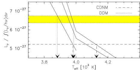
Figure 2: Range of effective temperatures derived with the Zanstra method for H in case of CDNM (dashed arows) and DDM (dotted arrows) for the $N_{\rm e,0}$ values of Fig. 1. The top boundary of the shaded region is for $N_{\rm e,0}=10^{2}$ cm^-3, the bottom boundary for $N_{\rm e,0}=10^{8}$ cm^-3. The solid lines are Kurucz models for the stellar $\log g=5.0;4.5;4.0$ (from right to left)

The range of possible effective temperature and surface gravity combinations of the central star derived with the Zanstra method for H is shown in Fig. 2 where we used Kurucz model atmospheres (Kurucz 1979) to calculate the left hand side of Eq. (2). While CDNM gives values in the range of $39\,800\leq T_{\rm eff}/{\rm K}\leq 41\,300$, the range found for DDM is shifted to lower values covering the range $38\,800\leq T_{\rm eff}/{\rm K}\leq 39\,850$; the lowest temperature is for the lowest (choosen) $N_{\rm e,0}$ value of $10^{2}$ cm^-3. The temperatures found with the two models are not extremely different; both methods result in a spectral type O for the central star of this compact planetary nebula.

Figure 3: Left: Constant electron density in CDNM derived from the observed (dashed line) sulfur line ratio. Right: The sulfur line ratios in case of DDM for $N_{\rm e,0}$ ranging from $10^{3}$ cm^-3 (lower left) to $10^{8}$ cm^-3 (upper right). The observed ratio (dashed line) limits $N_{\rm e,0}$ to values $\mathrel{\hbox{\hbox to0.0pt{\hbox{\lower 4.0pt\hbox{$\sim$}}\hss}\hbox{$>$}}}10^{5}$ cm^-3. The crossing point between model and observation defines the outer edge of the emitting shell for each model

3.2 Elemental abundances

We take for example the [Sii] lines and calculate for both models the intensity ratio of a [Sii] line over H$\beta$ (for details see e.g. Pottasch et al. 2003). For CDNM we need to know the constant electron density. This can be found from the sulfur line ratio (left panel of Fig. 3) and turns out to be $4\times 10^{4}$ cm^-3. The resulting ratio of the two Sii lines over H$\beta$ is shown in the left panel of Fig. 4. From this plot, a S⁺ abundance of $8.75\times 10^{-8}$ is found.

In case of DDM the observed sulfur line ratio defines the lower limit of $N_{\rm e,0}$ (right panel of Fig. 3) which is about $10^{5}$ cm^-3. Models with $N_{\rm e,0}<10^{5}$ cm^-3 cannot reproduce the observed line ratio of 2.25. In addition, the crossing point of the theoretical line ratio curve with the observed ratio defines the outer edge (in terms of $R_{0}$) of the emission shell for each density distribution model. This outer edge has to be taken into account when caclulating the intensity ratio of SII over H$\beta$. The results are shown in the right panel of Fig. 4. We find that the S⁺ abundance values calculated with DDM are all larger than the value found with CDNM, with the lowest value of $1.64\times 10^{-7}$ for $N_{\rm e,0}=10^{5}$ cm^-3 which is about twice the CDNM value.

Figure 4: Sii over H$\beta$ intensity ratio as a function of S⁺ abundance for CDNM (left) and DDM (right) for the different possible $N_{\rm e,0}$ values as indicated. Horizontal lines indicate observed ratios, arrows indicate the derived S⁺ abundance. All abundances found with DDM are clearly larger than that for CDNM

4 Conclusions

We derived the effective temperature and the S⁺ abundance for the Galactic compact PN Hen 2-90 using the constant density nebula approach and a shell model with a $r^{-2}$ density distribution. We find that the effective temperature of the central star derived with DDM is slightly (but not significantly) lower than with CDNM, classifying the star as spectral type O. The most interesting result is, however, that the S⁺ abundance found with DDM is definitely larger than the value found with CDNM. Even though we neglected additional ionization stages, this result might hold for all abundances derived from forbidden lines and might solve the problem of the underabundances sometimes found in PNe.

References

- (1) A. Ali: New Astronomy 4, 95 (1999)
- (2) R.D.D. Costa, J.A. de Freitas Pacheco, W.J. Maciel: A&A 276, 184 (1993)
- (3) R. Gruenwald, S.M. Viegas: ApJ 543, 889 (2000)
- (4) R.L. Kurucz: ApJS 40, 1 (1979)
- (5) S. Kwok, S., C.R. Purton, P.M. FitzGerald: ApJ 219, L 125 (1978)
- (6) D.E. Osterbrock: Physics of gaseous nebulae and active galactic nuclei (University science books, Mill Valley 1989)
- (7) J.P. Phillips: MNRAS 344, 501 (2003)
- (8) S.R. Pottasch: Planetary nebulae (D.Reidel Publishing Company, Dordrecht 1984)
- (9) S.R. Pottasch at al: A&A 409, 599 (2003)
- (10) L. Stanghellini et al: ApJ in press, astro-ph/0411631 (2004)
- (11) M. Steffen, D. Schönberner: Planetary Nebulae: Their Evolution and Role in the Universe, IAU Symposium 209, ed: S. Kwok, M. Dopita, R. Sutherland, (ASP, San Francisco, 2003), 439
- (12) E. Villaver, L. Stanghellini, R.A. Shaw: ApJ 597, 298 (2003)