Initial Ionization of Compressible Turbulence

Abstract

We study the effects of the initial conditions of turbulent molecular clouds on the ionization structure in newly formed H ii regions, using three-dimensional, photon-conserving radiative transfer in a pre-computed density field from three-dimensional compressible turbulence. Our results show that the initial density structure of the gas cloud can play an important role in the resulting structure of the H ii region. The propagation of the ionization fronts, the shape of the resulting H ii region, and the total mass ionized depend on the properties of the turbulent density field. Cuts through the ionized regions generally show “butterfly” shapes rather than spherical ones, while emission measure maps are more spherical if the turbulence is driven on scales small compared to the size of the H ii region. The ionization structure can be described by an effective clumping factor $\zeta=\langle n\rangle\cdot\langle n^{2}\rangle/\langle n\rangle^{2}$, where $n$ is number density of the gas. The larger the value of $\zeta$, the less mass is ionized, and the more irregular the H ii region shapes. Because we do not follow dynamics, our results apply only to the early stage of ionization when the speed of the ionization fronts remains much larger than the sound speed of the ionized gas, or Alfvén speed in magnetized clouds if it is larger, so that the dynamical effects can be negligible.

1. INTRODUCTION

H ii regions are photoionized regions surrounding young OB stars. The ionization structures and physical properties of these regions are important to understanding of the formation of massive stars and their feedback to the environment. Over the past several decades, H ii regions have been extensively observed in various size and shapes (e.g. see reviews by Wood & Churchwell 1989; Garay & Lizano 1999; Churchwell 1999, 2002). Depending on their sizes, they are usually classified as ultracompact (linear size below 0.1 pc), compact (0.1–1 pc), or extended (several to tens of parsecs). Ultracompact and compact H ii regions are ionized by massive stars still embedded in their natal molecular clouds, while extended H ii regions are thought to be in their mature states, powered by a combination of stellar radiation, stellar wind and supernova explosions in the associated OB star clusters (Yang et al. 1996). Despite the diversity of sizes, H ii regions generally display common features such as inhomogeneities and irregular shapes. One interesting and still open question on the origin of these complex structures is: are they from the initial conditions of the gas before ionization, or formed by dynamical processes during H ii region evolution?

Early analytical and numerical work focused on the formation of H ii regions and the propagation of ionization fronts (I-fronts), by modeling the ionization of a massive star suddenly turned on in a uniform gas (Stromgren 1939; Kahn 1954; Axford 1961; Goldsworthy 1961; Tenorio-Tagle 1976; Elmegreen 1976). It was soon realized, however, that the interstellar medium is far from homogeneous. Simple condensations or smooth variations of density were then included in some model calculations (Flower 1969; Marsh 1970; Kirkpatrick 1970, 1972; Pequignot, Stasinska & Aldrovandi 1978; Köppen 1979; Icke 1979; Tenorio-Tagle & Bedijn 1981, see Yorke 1986 for a review). However, in the early studies, radiative transfer effects were either ignored in calculations or limited to one or two-dimensional treatments, and suffered from low resolutions (Sandford 1973; Klein, Stein & Kalkofen 1978; Köppen 1978; Tenorio-Tagle 1979; Sandford, Whitaker & Klein 1982), which limited their applications to observations.

Recently, several authors have reported two-dimensional simulations of the dynamical evolution of H ii regions and their applications to observations. García-Segura & Franco (1996) presented two-dimensional gasdynamical simulations of the evolution of H ii regions in constant and power-law density profiles, and argued that a thin-shell instability of the ionization fronts could produce the irregular and bright edges of the H ii region. Williams (1999) also performed two-dimensional gasdynamical simulations and showed that shadowing instability could also lead to formation of dense clumps. Freyer, Hensler, & Yorke (2003) presented two-dimensional radiation gasdynamical simulations of the interaction between an isolated massive star and its homogeneous and quiescent ambient ISM, and showed that the redistribution of mass by the action of the stellar wind shell could form the “finger-like” shapes.

However, since star forming regions display a wide range of kinematic properties and density distributions, the gas may well be turbulent, clumpy, filamentary, and coupled with the magnetic field (Elmegreen 1993; Dyson, Williams & Redman 1995; Redman et al 1998; Mac Low 1999; Crutcher 1999; Williams, Dyson & Hartquist 2000; Klessen, Heitsch, & Mac Low 2000; Ostriker, Stone, & Gammie 2001; see Mac Low & Klessen 2004 for a recent review). These uniform models may not capture the realistic density field of the ambient medium. The initial inhomogeneities and turbulent structures of the gas clouds may affect the propagation of the ionization fronts and contribute to the shaping of the resulting H ii regions.

To test this, a reliable, three-dimensional treatment of radiative processes is essential, and high resolution simulations of radiative transfer fully coupled with gasdynamics in turbulent medium are highly desirable. However, incorporating radiative transfer in gasdynamics simulation presents a serious numerical challenge. The difficulties are due to the non-locality of the radiation physics, which hampers efficient parallelization of the simulations and severely limits the size of problem that can be tackled. So far most calculations have not been able to include transfer of ionizing radiation into three-dimensional gasdynamics simulations, so, as a step forward to investigate the ionization of turbulent clouds, we apply radiative transfer to a static, pre-computed, three-dimensional, turbulent density field. It is a simplified model, but so long as the speed of the I-front is much larger than the sound speed of the ionized gas, the expansion of the gas can be neglected (Spitzer 1978), and the density field can be treated as static. In cases where a magnetic I-front is considered (e.g. Williams, Dyson & Hartquist 2000), the Alfvén speed in the mostly neutral gas ahead of the I-front should replace the ionized sound speed in the above criterion if it is larger. However, usually the ionized sound speed dominates.

As we will show, this simple approach produces a variety of interesting morphological structures that may provide us some understanding of the physical processes in H ii regions even before more sophisticated calculations can be performed. However, our results only apply to the initial photoionization of static turbulence before gasdynamics becomes important, so future comprehensive simulations with a full treatment that couples radiative transfer and gasdynamics will be necessary to confirm and extend them.

We present high resolution computations of the initial ionization of compressible turbulence by a point ionizing source, such as a young star. We apply INONE, a three-dimensional radiative transfer code developed by Abel (2000), to a compressible turbulent medium from different hydrodynamical (HD) and magnetohydrodynamical (MHD) models using ZEUS-3D (Stone & Norman 1992a, b), as described in Mac Low (1999). INONE integrates the jump condition of I-fronts, and uses a photon-conserving method that is independent of numerical resolution and ensures correct propagation speeds for the I-fronts (Abel, Norman & Madau 1999). In §2 we briefly describe the methods of computation, and the codes and models used in this work; we present the results of propagation of I-fronts, emission measure maps, and ionization structures in §3; and in §4 we give an analytical discussion of the key parameters that determine the ionization structure, as well as the validity of the assumptions.

2. COMPUTATIONS

2.1. Compressible Turbulent Molecular Clouds

Star forming molecular clouds have been observed to be highly clumpy and have broad emission line widths, which suggests supersonic motions in the clouds (Blitz 1993). These supersonic motions seem not to be ordered. Crutcher (1999) presented Zeeman observations of magnetic fields in molecular clouds that showed that velocities in the observed clouds are typically Alfvénic. So molecular clouds are generally self-gravitating, clumpy, magnetized, turbulent, compressible fluids. Although numerical simulations of transient, compressible turbulent molecular clouds have been carried out for several years, we are far from drawing a comprehensive picture of the complicated structure of the clouds.

Mac Low (1999) conducted direct numerical computations of uniform, randomly driven turbulence with $128^{3}$ resolution using the ZEUS-3D MHD code , which successfully simulated the density distribution of the turbulent medium. ZEUS-3D is a well-tested, Eulerian, finite-difference code (Stone & Norman 1992a, b; Clarke & Norman 1994). It uses second-order van Leer (1977) advection and resolves shocks using von Neumann artificial viscosity. It also includes magnetic fields in the MHD approximation (Hawley & Stone 1995). Falle (2002) pointed out some problems with ZEUS: rarefaction waves often break up into a series of jumps, and adiabatic MHD shocks sometimes show errors. However, as we are using isothermal MHD, and are primarily concerned with the density field, which is barely affected by rarefaction shocks, our models remain valid.

Table 1Turbulence Models (Mac Low 1999)

$Model$	$\dot{E_{\rm in}}$	$k$	$C$
HA8	0.1	8	1.50
HC2	1	2	5.88
HC4	1	4	4.89
HC8	1	8	2.97
HE2	10	2	7.24
MA81	0.1	8	1.46
MC41	1	4	2.46
MC45	1	4	4.35
MC4X	1	4	5.88
MC81	1	8	2.46

For our computations, we assemble $384^{3}$ density fields by repeating the periodic $128^{3}$ models of Mac Low (1999). Table 1 describes the models we use. The model names begin with either “H” for hydrodynamic or “M” for MHD, then have a letter from “A” to “E” specifying the level of energy input $\dot{E_{\rm in}}$, then a number giving the dimensionless wave-number $k$ chosen for driving, and then, for the MHD models, another number indicating the initial field strength specified by the ratio of Alfvén speed to the sound speed. In the last column, $C$ is the gas clumping factor defined as $C=\langle n^{2}\rangle/\langle n\rangle^{2}$. Note that the values of $C$ listed here are averaged over the whole simulated volume.

2.2. Ionization Front Tracking

In general, a study of the evolution of ionization zones around a ionizing source requires a full solution to the radiative transfer equation (Kirchhoff 1860):

$$\frac{1}{c}\frac{\partial I_{\rm\nu}}{\partial t}+\hat{n}\cdot\nabla I_{\rm\nu}=\eta_{\rm\nu}-\chi_{\rm\nu}I_{\rm\nu}\,,$$ (1)

where $\hat{n}$ is a unit vector along the direction of the radiation, $I_{\rm\nu}$ is the monochromatic specific intensity of the radiation field, and $\eta_{\rm\nu}$ and $\chi_{\rm\nu}$ are emission and absorption coefficients, respectively.

However, a direct solution of equation (1) is usually impractical because of its high dimensionality. Abel, Norman & Madau (1999) made the calculations feasible by developing a ray tracing algorithm for radial radiative transfer around point sources, reducing the dimensionality of the transfer equation to a level where ionization can be computed on a Cartesian grid. This algorithm conserves energy explicitly and thus gives the right speed of I-fronts, but ignores the diffuse field produced by scattered radiation.

Kahn (1954) defined the nomenclature of $R$ (“rarefied”) and $D$ (“dense”) fronts according to the speed of the I-fronts with respect to the sound speed of the ionized gas: R-type fronts move supersonically while D-type fronts move subsonically. If a source of ionizing radiation suddenly switches on, the I-front is initially weak R-type. Once its velocity drops to about twice the sound speed in the ionized gas, the I-front becomes D-type (Dyson et al. 2002). The propagation of an R-type I-front in a static medium is given as:

$$4\pi R_{\rm I}^{2}n_{\rm{H}}(R_{\rm I})\frac{dR_{\rm I}}{dt}=F-\int_{0}^{R_{\rm I}}\alpha_{\rm B}4\pi r^{2}n_{\rm p}(r)n_{\rm e}(r)\ dr\,.$$ (2)

where $R_{\rm I}$ is the radius of the I-front, $F$ is the ionizing photon flux, $n_{\rm H}$, $n_{\rm p}$ and $n_{\rm e}$ are the number density of the neutrals, ions, and electrons, respectively. We assume a constant case B recombination rate, $\alpha_{\rm B}=2\times 10^{-13}$ cm³ s^-1 for $T\sim 10^{4}$ K. Integrating equation (2) along the rays with the ray-tracing technique mentioned above gives the time at which the ionization front arrives at a given cell, as is done in INONE (Abel 2000). Retrieving the arrival time in a 3D array allows one to investigate the time dependent morphology of the I-fronts.

2.3. Scaling

In this paper, we use INONE to compute photoionization of different turbulence models. For simplicity, we consider hydrogen gas only. We expect the inclusion of helium to have only a minor effect on the results presented here. The simulations are scale free and depend only on the ionizing flux $F$ and density $n$ of the medium, so one can derive the scaling of physical parameters such as ionized mass $M$, ionized volume $V$, and ionization time $t$ in terms of $F$ and $n$. As the analytical derivation in §4.1 demonstrates, the ionized mass at late times scales as $M\propto F/n$; the ionized volume at late times is close to the volume of the Strömgren sphere, and scales as $V\propto F/n^{2}$; and the characteristic timescale is the recombination time, which scales as $t\propto 1/n$. As an example, if we choose $F_{0}=1.2\times 10^{49}$ s^-1, which is typical for an O6 star (Panagia 1973), and a cloud with a size of 0.5 pc and average density of $n_{0}=5\times 10^{3}$ cm^-3, we then have $M_{0}=10M_{\odot}$, $V_{0}=0.08$ pc³, and $t_{0}=10^{11}$ s (these will be given in §3 as the results of the simulations). For given F and n, one can rescale our results as follows:

$$M_{0}^{\prime} = \left(\frac{F}{F_{0}}\right)\left(\frac{n}{n_{0}}\right)^{-1}M_{0}$$ (3)

$$= (10\ M_{\odot})\left(\frac{F}{1.2\times 10^{49}\ s^{-1}}\right)\left(\frac{n}{5\times 10^{3}\ cm^{-3}}\right)^{-1}\,,$$

$$V_{0}^{\prime} = \left(\frac{F}{F_{0}}\right)\left(\frac{n}{n_{0}}\right)^{-2}V_{0}$$ (4)

$$= (0.08\ pc^{3})\left(\frac{F}{1.2\times 10^{49}\ s^{-1}}\right)\left(\frac{n}{5\times 10^{3}\ cm^{-3}}\right)^{-2}\,,$$

$$t_{0}^{\prime} = \left(\frac{n}{n_{0}}\right)^{-1}t_{0}$$ (5)

$$= (10^{11}\ s)\left(\frac{n}{5\times 10^{3}\ cm^{-3}}\right)^{-1}\,.$$

In the simulations, we use the pre-computed gas density distribution with ZEUS-3D for the HD and MHD models listed in Table 1 as input into INONE. We will discuss the validity of this treatment later in §4.2. Three simulations are conducted for each model, by varying the position of the star to the maximum density, minimum density, or center of the density field (random density), so for our example a total of 30 simulations were performed on SGI Origin2000 computers. Each computation took several days on a single processor.

3. RESULTS

3.1. Shapes of the Ionized Regions

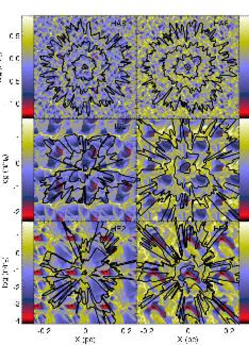
Figure 1.— Propagation of an R-type I-front in a $384^{3}$ density field simulated with different HD models. The ionizing source is located at maximum (left), and minimum density (right), respectively. The contours give the position of the I-front from 0.1 yr to 100 yr, with the interval increasing evenly by a factor of 10. The size of box is 0.5 pc, $\langle n_{0}\rangle=5\times 10^{3}$ cm^-3. Note the image and contour are slices through middle point of the cube.

Figures 1 and 2 show the propagation of the I-fronts into the turbulent medium surrounding a point source. The background image is the density distribution of the gas simulated by HD and MHD models, respectively. The contours are the arrival times of the I-fronts. In Figure 1, the density fields are taken from HD models with different energy input and driving wave number, while in Figure 2, the density fields are from MHD models with different driving wave number and magnetic field strength, as listed in Table 1. In both figures, the left panels are for the case that the point source (star) is placed at the maximum density, while in the right panels the star is placed at the minimum density. In each individual panel, the contours give the position of the I-fronts in our example scaling from 0.1 to 100 years, with the interval increasing evenly by a factor of 10. The models chosen in each figure have different average clumping factors (see Table 1).

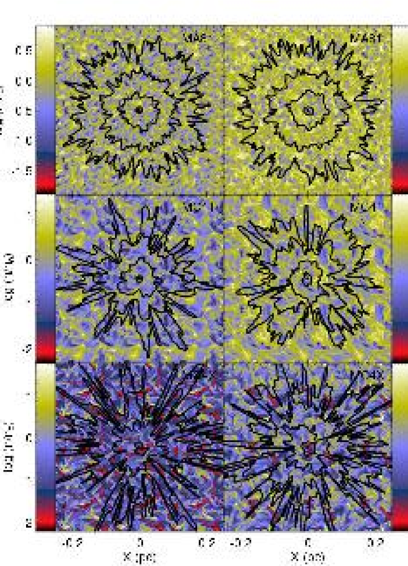
Figure 2.— Propagation of the I-front in a $384^{3}$ density field simulated with different MHD models. The ionizing source is located at maximum (left), and minimum density (right), respectively. The contours give the position of the I-front from 0.1 to 100 years, with the interval increasing evenly by a factor of 10. The size of box is 0.5 pc, $\langle n_{0}\rangle=5\times 10^{3}$ cm^-3. Note the image and contour are slices through middle point of the cube.

At early times, the recombination term in equation (2) can be neglected, and the I-front velocity is determined by the local density structure of the gas: the front travels faster into voids and slower into denser filaments. The shape of the I-front depends on the size and contrast of the voids and clumps. Longer turbulent driving wavelengths (smaller driving wave numbers) create structure in the density field on larger scales and produce more asymmetric H ii regions with characteristic ’butterfly’ shapes. At later times, recombination becomes significant, increasing the dependence on local density and making the resulting asymmetry more pronounced.

The initial I-front velocity is sensitive to the placement of the ionizing point source, as can be seen from a comparison of the innermost contours in the left-hand and right-hand columns of Figures 1 and 2. However, this effect becomes less important at later times, and the final H ii regions of the same model have very similar sizes, regardless the position of the ionizing source, as can be seen in Figures 6.

In Figures 1 and 2, the images are sorted in order of increasing clumping factor $C$; e.g. in Figure 1 $C(\rm HA8)=1.5$, $C(\rm HC2)=5.88$, $C(\rm HE2)=7.24$, and similar trend in Figure 2. Comparison of the images clearly shows a strong link between the size of the clumping factor and the morphology of the H ii region – the larger the clumping factor, the more asymmetric the H ii region becomes.

3.2. Emission Measure

For comparison with observations, we can map the emission measure in our models,

$$EM=\int n_{\rm e}^{2}dl$$ (6)

where $l$ is the size of the region along the line-of-sight. Typically more compact H ii regions have higher emission measures. For example, an extended H ii region with size of 10–100 pc and density of 10 cm^-3 has EM in the range of 10^3-4 pc cm^-6, while an ultracompact H ii region with size $<0.1$ pc and density $\geq 10^{4}$ cm^-3 is brighter, with EM $>10^{7}$ pc cm^-6.

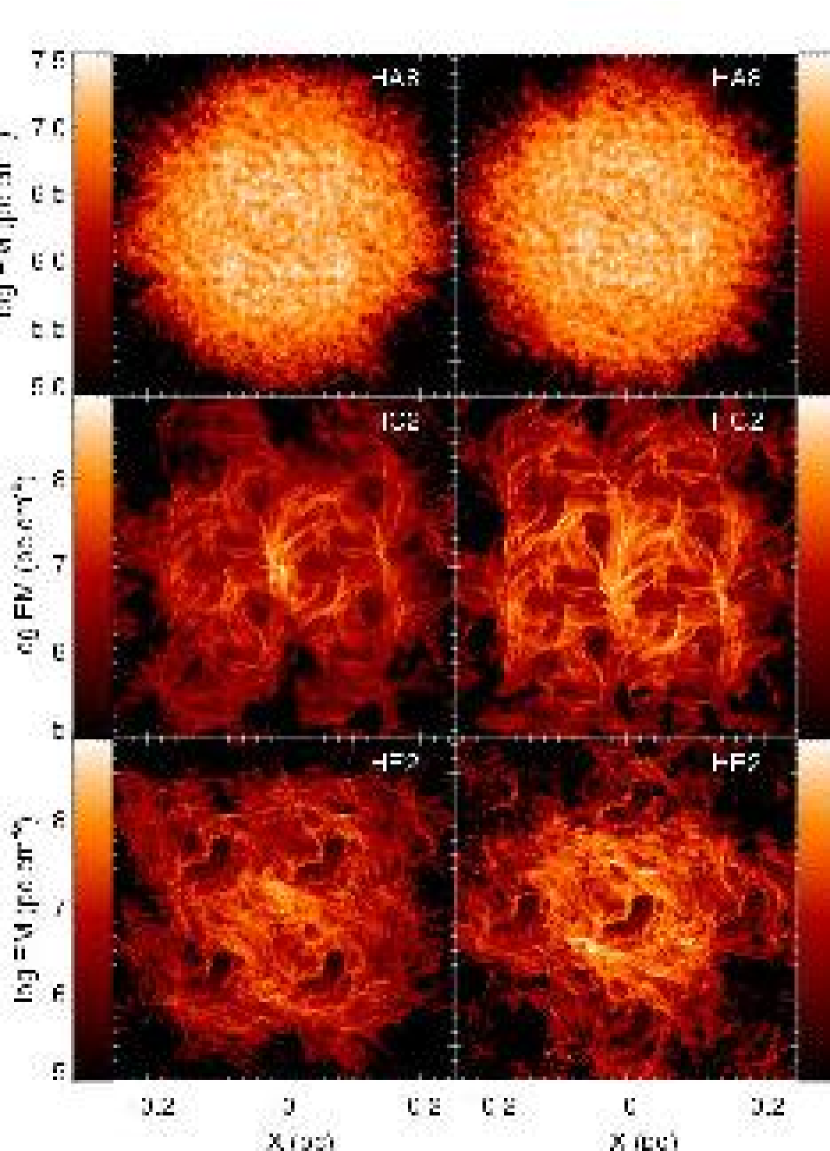
Figure 3.— Emission measure of the ionized regions of HD models at $t\simeq 100$ yr, assuming the scales used in the text as an example. The ionizing source is located at maximum (left), and minimum density (right), respectively.

We calculate emission measure maps from the simulations by integrating density $n_{H}^{2}$ of the ionized regions through the path length in the third direction. Figures 3 and 4 show emission measure maps in the x-y plane of HD and MHD models, respectively. The arrangement of the models in both figures are the same as in Figures 1 and 2. We can see that the range of the EM is around $10^{6-8}$ pc cm^-6 for our adopted parameters, which agrees, as expected, with the observed range of compact H ii regions.

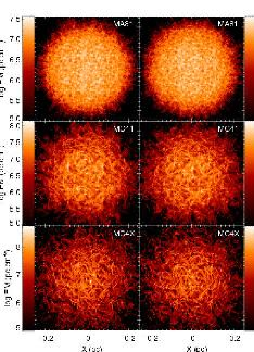
Figure 4.— Emission measure of the ionized regions of MHD models at $t\simeq 100$ yr assuming the scales used in the text as an example. The ionizing source is located at maximum (left), and minimum density (right), respectively.

The shape and structure of the EM map depends on the clumping factor: the smaller the clumping factor is, the more spherical the map appears. Filamentary structures and contrast within the H ii region also increase with $C$. There are some differences between the HD and MHD models with $C>1$: HD models tend to have more irregular shapes, and bigger voids and clumps. Larger driving wavelengths of the turbulence also produce larger voids and clumps. These results generally suggest that the turbulent structures observed in H ii regions may be driven at large scale, and that the initial gas clouds may have a large clumping factor. However, the influence of dynamics will have to be computed to put any such conclusion on a firm basis.

3.3. Ionization Structure

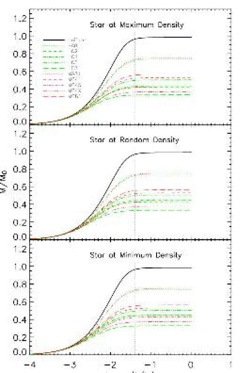
Figure 5.— Ionized mass over time for different models, with ionizing star at (top:) maximum density, (middle:) a random position, and (bottom:) minimum density. $M_{0}$ and $t_{0}$ are defined in §2.3. The vertical dashed line indicates the minimum time when $v_{\rm if}=2c_{s}$ (see Figure 10).

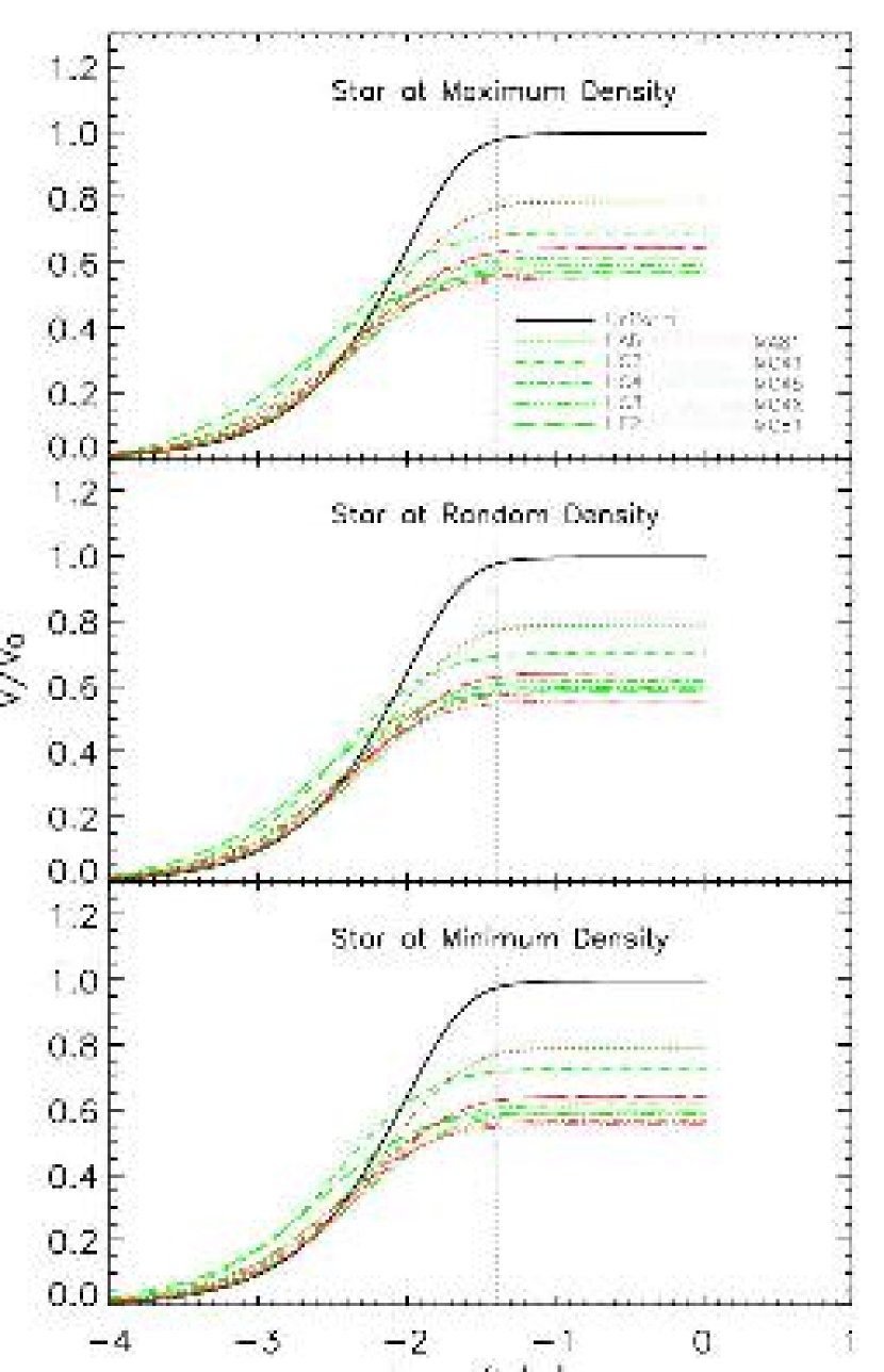
Figure 6.— Ionized volume over time for different models, with ionizing star at (top:) maximum density, (middle:) a random position, and (bottom:) minimum density. $V_{0}$ and $t_{0}$ are defined in §2.3. The vertical dashed line indicates the minimum time when $v_{\rm if}=2c_{s}$ (see Figure 10).

Figures 5 and 6 show the time-dependent ionized mass and ionized volume, respectively. Note that the units, $M_{0}$, $V_{0}$, and $t_{0}$ are the same as in equations (3), (4), and (5). Different panels have the ionizing star at different positions, while within each panel, different curves indicate different models. The ionized volume is calculated by integrating the ionized cells at time t, and the ionized mass is the integral of the mass encompassed in the ionized volume. The curves become saturated around $t\sim 100$ years. It appears that the mass of the ionized gas in our example is close to that of a compact H ii region (Franco et al. 2000). For the same input energy strength and driving wave number, no big difference is seen between the MHD and the HD models. However, all the curves follow a sorted order of the clumping factor $C$, with HA8 and MA81 having the smallest $C$, while HE2 has the largest $C$.

3.4. Compared With Two-Phase Clumpy Model

Here we compare our results with an analytic model of a two-phase clumpy medium. Consider a medium with optically thin clumps of number density $n_{\rm cl}$ in a uniform density field of number density $n_{\rm bg}$, which was studied by Köppen (1979). If we take a filling factor $\epsilon$ for clumps, and the density contrast $\xi=n_{\rm bg}/n_{\rm cl}$, then the average density is:

$$\bar{n}=\epsilon n_{\rm cl}+(1-\epsilon)n_{\rm bg}=n_{\rm cl}\left[\epsilon+(1-\epsilon)\xi\right]\,,$$ (7)

The ionization structure of this medium is:

$$4\pi R_{\rm I}^{2}\bar{n}\frac{dR_{\rm I}}{dt} = F-\int_{0}^{R_{\rm I}}4\pi r^{2}\alpha_{\rm B}n_{\rm cl}^{2}\epsilon dr$$ (8)

$$-\int_{0}^{R_{\rm I}}4\pi r^{2}\alpha_{\rm B}n_{\rm bg}^{2}(1-\epsilon)dr\,,$$

where $\alpha_{\rm B}$ is the recombination-rate coefficient as in equation (2). Define a two-phase clumping factor $C_{2}$,

$$C_{2}=\frac{\epsilon+(1-\epsilon)\xi^{2}}{\epsilon\xi+(1-\epsilon)\xi^{2}}\,,$$ (9)

and define $dN=4\pi R_{\rm I}^{2}\bar{n}dR_{\rm I}$, where $N$ is the total number of ions. Equation (8) can then be written as

$$\frac{dN}{dt}=F-\alpha_{\rm B}C_{2}n_{\rm bg}N\,,$$ (10)

from which we get an analytical solution of the number of the ions N, and the ionized mass $M_{\rm{2}}$:

$$M_{2}=m_{p}\cdot N=\frac{F}{\alpha_{\rm B}C_{2}n_{\rm bg}}(1-e^{-\alpha_{\rm B}C_{2}n_{\rm bg}t})\,.$$ (11)

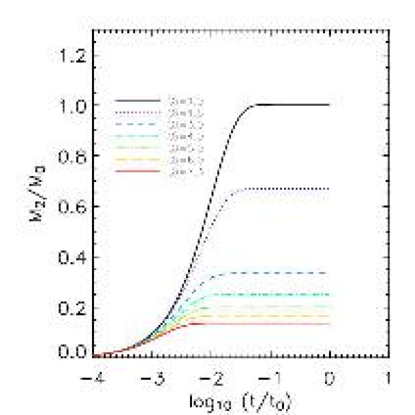
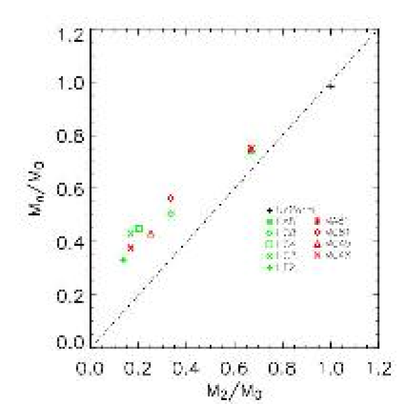
Figure 7.— Left: ionized mass of two-phase clumpy model over time for different two-phase clumping factors $C_{2}$ taken after the values of the turbulence models in Table 1. Right: comparison of numerical ionized mass $M_{n}$ (the ionizing star is located at random position) to analytical ionized mass from the two-phase models $M_{\rm{2}}$. Note that the dotted line in this plot is not a fitting curve, but just a diagonal line to guide the eyes.

Figure 7 shows the ionized mass from the two-phase model, and a comparison between the analytical results and the numerical ones. The clumping factors $C_{2}$ were chosen to be close to the values measured in the turbulence simulations, as listed in table 1. From top to bottom in the plot, we have 1.0 (uniform gas), 1.5, 3.0, 4.0, 5.0, 6.0 and 7.3 respectively. The background density $n_{\rm bg}$ is taken as the mean density $n=5\times 10^{3}$ cm^-3 of the scaled simulations. Though similar in shape, the results of the two-phase model are distinct from those of the turbulent models; the ionized mass for a given $C_{2}$ is less than in the corresponding turbulent model, and the difference increases as the medium becomes more clumpy.

4. DISCUSSION AND SUMMARY

We have presented simulations of different models, and found that a two-phase clumpy model can not fully describe the ionization structure of the turbulence models. However, some questions still remain: what determines the ionization structure? When are our assumptions valid?

4.1. What Determines the Ionization Structure?

The results shown above suggest that the ionization structure is sensitive to the input energy strength and driving wave number of the turbulence. But qualitatively, what is the key factor that determines the ionization structure?

Assume the density field is constant, and the gas is fully ionized within the ionization front, then both the ion density $n_{\rm p}(r)$ and the electron density $n_{\rm e}(r)$ at radius $r$ are equal to the original hydrogen density $n(r)$, $n_{\rm p}(r)=n_{\rm e}(r)=n(r)$. Let $N(t)$ be the total number of the ions at time t, $N(t)=\int_{0}^{R_{\rm I}}n(r)\ dV$, then equation (2) can be rewritten as:

$$\frac{dN(t)}{dt} = F-\alpha_{\rm B}\int_{0}^{R_{\rm I}}n(r)^{2}\ dV$$ (12)

$$= F-\alpha_{\rm B}\cdot\langle n\rangle\cdot\frac{\langle n^{2}\rangle}{\langle n\rangle^{2}}\cdot N(t)\,.$$

We can now see that the ionized mass depends explicitly on the average gas density $\langle n\rangle$, and the local clumping factor ($C=\langle n_{H}^{2}\rangle/\langle n_{H}\rangle^{2}$) within the I-front. Different driving strength and wave number of the turbulence yield different size and contrast of clumps and voids, which is represented by $C$ and $\langle n\rangle$, thus yielding different ionization structures. Since $R_{\rm I}$ changes with time, we further define an effective clumping factor $\zeta(t)=\langle n\rangle\cdot\langle n^{2}\rangle/\langle n\rangle^{2}$, so that equation (12) can be rewritten as:

$$\frac{dN(t)}{dt}=F-\alpha_{\rm B}\cdot\zeta(t)\cdot N(t)\,.$$ (13)

From this we can see that $\zeta$ describes the density field, and determines the ionized mass. Figure 8 shows $\zeta$ as a function of time for our models. Comparing Figure 8 with Figure 5, we find that the order of the models in Figure 8 is exactly the inverse order in Figure 5. The larger the $\zeta$, the less mass is ionized, as predicted from equation 13.

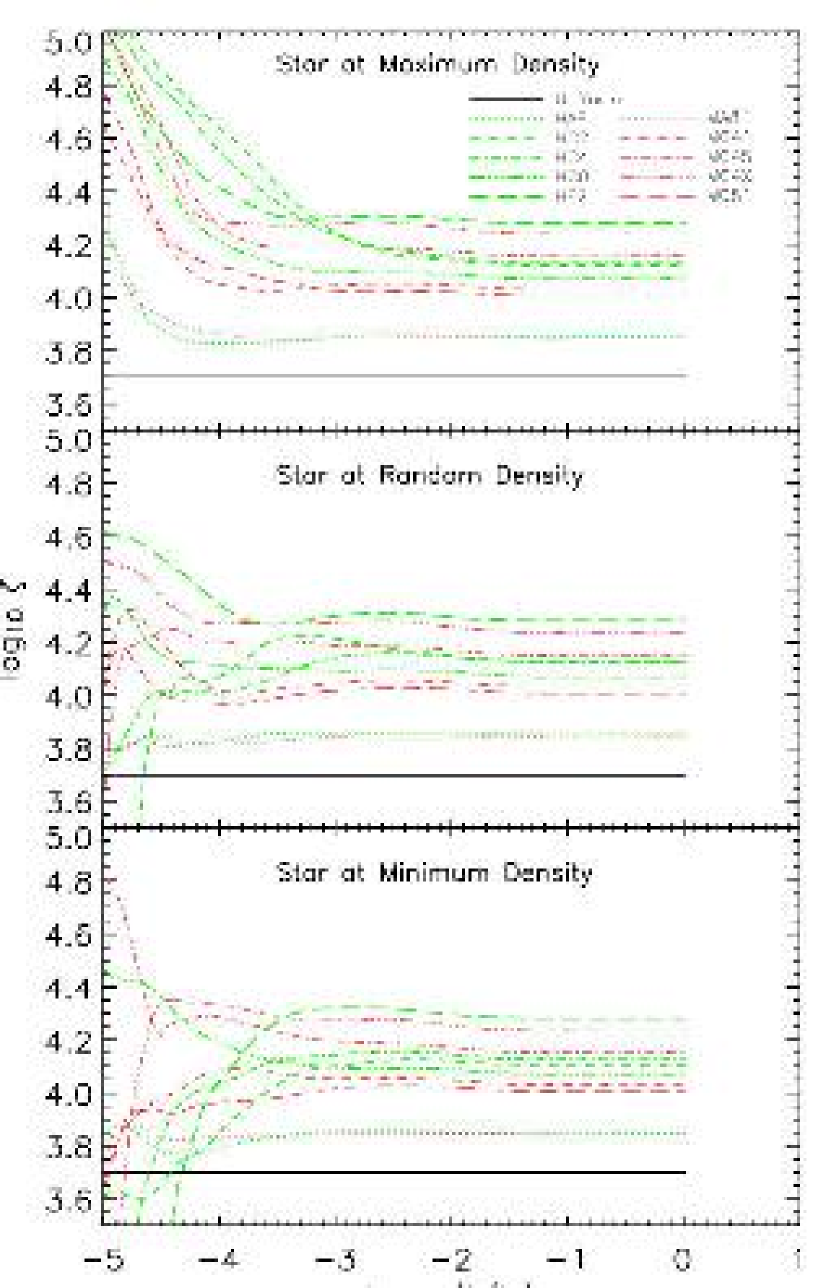
Figure 8.— Effective clumping factor $\zeta$ versus time as an indicator of ionization structure. It varies with different models, and different position of the ionizing star at (top:) maximum density, (middle:) a random position, and (bottom:) minimum density.

The dependence of the effective clumping factor $\zeta(t)$ on the density field is nontrivial because the averaging volume is itself a time-dependent function of the density field. However, $\zeta$ tends to saturate once the radius of the I-front is larger than the turbulence driving scale. This also corresponds to the saturation of the photoionization. The total ionized mass can then be approximated well with equation 13. Note also that in these figures, different positions of the ionizing star does not make much difference, because $\zeta$ is a measure of the density field, and the ionized mass depends only on $\zeta$ and the ionizing flux, no matter where the source is. In turbulence simulations, resolution might affect the value of $\zeta$, but it would not affect our result as a function of $\zeta$.

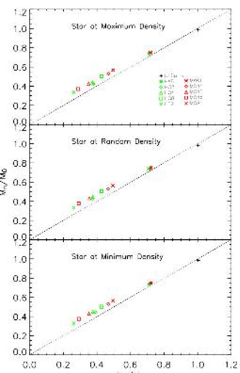
Figure 9.— Comparison of numerical ionized mass $M_{n}$ to analytical ionized mass $M_{a}$ for different models, and different position of the ionizing star at (top:) maximum density, (middle:) a random position, and (bottom:) minimum density. Note that the dotted lines in the plots are not fitting curves, but just diagonal lines to guide the eyes.

Figure 9 shows a comparison of numerical and analytical values of ionized mass for the different models. The small variance between numerical simulations and analytical calculations suggests that the calculations are self-consistent, and that the numerical resolution of the calculation is good enough to resolve the structure. Since in reality the density fields are more complicated than the simplified model used in the analytical calculations, there is a systematic difference between the numerical results and the analytical ones: in all these models, the smaller the clumping factor, the smaller the difference.

4.2. When Are the Assumptions Valid?

In the above simulations, the density field of the gas is simulated beforehand and then input to INONE, so gasdynamics is not computed simultaneously during the course of radiative transfer. However, when the speed of the I-fronts slows to roughly twice the sound speed of the ionized gas, the expansion of the gas will dominate the evolution of the region, and gasdynamics must be considered (Spitzer 1978). Figure 10 shows the time evolution of the ratio of speed of I-fronts $v_{\rm if}$ to sound speed $c_{s}$, $v_{\rm if}/c_{s}$, for different models. The sound speed is $c_{s}=9.1$ km s^-1 for $T=10^{4}$ K. The velocity of the I-fronts, $v_{\rm if}=dR_{i}/dt$, is hard to derive because it is three dimensional, and even at the same photon arrival time, it may vary dramatically in different cells if the local clumping factors are different, so what is shown here is an average value at $R_{i}$, the radius of the I-front at time t. However, one should keep in mind that in some regions $v_{\rm if}$ may be much smaller than the average value. For example, an obliquely propagating ionization front moves slowly and transitions from R-type to D-type more quickly (Williams 1999). Fully dynamical simulations are necessary to assess the impact of these effects. From Figure 10, we can see that the speed of I-fronts decreases rapidly with time, and at about log${}_{10}(t/t_{0})=-1.4$ (which corresponds to $t\sim 100$ years in our example), it drops to twice of the sound speed, so after this time the simulations are likely unreliable. From Figure 5 and 6, we can see that this is the time when the curves of ionized mass and ionized volume become saturated, so the details of the ionization structure derived up to that point are likely reliable.

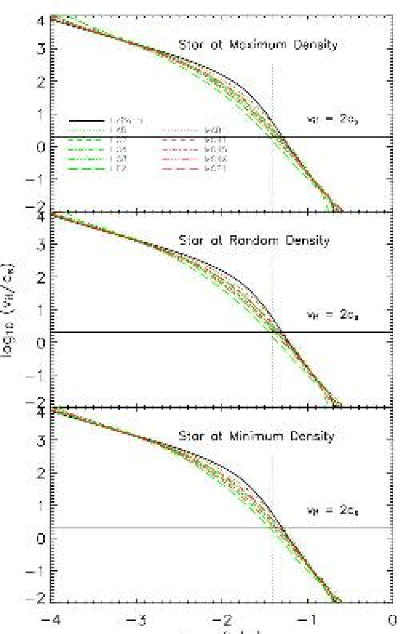
Figure 10.— Time evolution of $v_{\rm if}/c_{s}$, ratio of speed of I-fronts $v_{\rm if}$ to sound speed $c_{s}$, for different models. When $v_{\rm if}$ decreases to twice of the sound speed, expansion of the ionized gas is significant. The vertical dashed line indicates the minimum time at when $v_{\rm if}=2c_{s}$.

Williams, Dyson & Hartquist (2000) presented one-dimensional simulations on jump conditions of magnetic I-fronts and showed that fast R-type I-fronts could decrease quickly to slow D-type I-fronts in oblique magnetic fields. We note, however, that as long as the propagation speed of the I-fronts is much larger than the Alfvén speed of the medium, this effect remains unimportant. In molecular clouds, the typical Alfvén speed is about 1–5 km s^-1, which is no larger than the sound speed in ionized gas. Table 1 shows that the ratio of Alfvén speed to the sound speed in the MHD models is appropriate for cold, molecular clouds. Crutcher (1999) showed an empirical power-law relationship between magnetic field strength and density above $10^{3-4}$  cm^-3. According to this scaling law, our density field ($\langle n\rangle=5000$ cm^-3) might have $B\sim 50\ \mu G$, which gives an Alfvén velocity $v_{A}=(B^{2}/(4\pi\rho))^{1/2}\sim 5$ km s^-1. The ionized sound speed $c_{s}=9.1$ km s^-1, larger than the Alfvén speed $v_{A}$, which suggests that our critical point log${}_{10}(t/t_{0})=-1.4$ occurs before the magnetic field becomes important.

Again, it should be emphasized that our simulations are simplified models in which a point ionizing source is turned on in a static turbulent density field. We did not take into account several effects, such as the mass accretion by the ionizing star, the diffuse field, and any time evolution in the ionizing luminosity of the star (Yorke 1986). These effects should eventually be included in more comprehensive future simulations. Our main focus here is to investigate how the initial conditions of the gas affect the ionization structures of the resulting H ii region.

4.3. Summary

We have presented a study of the effects of turbulent initial conditions on the ionization structures of young H ii regions. We performed high resolution, three-dimensional radiative transfer computations, as well as analytical calculations, of the propagation of I-fronts into static density distributions drawn from numerical simulations of compressible, turbulent molecular clouds. Our results show that the initial turbulent structure of the gas can play an important role in the early ionization structure. The propagation of the I-fronts, the shape of the resulting H ii regions, and the total mass ionized depend on the local strength of the voids and clumps. We can characterize this with an effective clumping factor $\zeta=\langle n^{2}\rangle/\langle n\rangle$. The ionization fronts move quickly into voids but slowly into dense filaments. The ionized mass changes inversely with $\zeta$. Cuts through the ionized regions generally have “butterfly” shapes, with larger $\zeta$ producing more irregular shapes. Larger scale driving of the turbulence produces more filamentary emission measure maps.

We emphasize that our results are based on static density fields, so they apply only to the early stages of the evolution of an H ii region when the speed of the ionization fronts remains much larger than the sound speed of the ionized gas, so that the expansion of the gas is negligible. (In cases where magnetic field is considered, the neutral Alfvén speed should be used in addition to the ionized sound speed, but it is rarely higher.) We regard our results as complementary to the findings of García-Segura & Franco (1996), Williams (1999), and Freyer, Hensler, & Yorke (2003), who study the dynamical evolution of H ii regions with two-dimensional simulations, but only with uniform or smoothly varying initial conditions. Future comprehensive simulations with a full treatment that couples gas dynamics and radiative transfer, and with realistic initial conditions, will be necessary to extend these results to later times.

References

- Abel, Norman & Madau (1999) Abel, T, Norman, M. L. & Madau, P. 1999, ApJ 523, 66
- Abel (2000) Abel, T. 2000, Rev. Mex. Astro. Astrof. Ser. Conf. 9, 300
- Axford (1961) Axford, W. I. 1961, Philos. Trans. R. Soc. London Ser. A 253, 301
- Blitz (1993) Blitz, L. 1993 Protostars & Planets III, ed. E. H. Levy & J. I. Lunine (Tucson: Univ. of Arizona Press), 125
- Churchwell (1999) Churchwell E. 1999 In The Origin of Stars and Planetary Systems, ed. CJ Lada, ND Kylafis, Dordrecht, The Netherlands: Kluwer, pp. 515-52.
- Churchwell (2002) Churchwell E. 2002, ARAA 40, 27
- Clarke & Norman (1994) Clarke, D. & Norman, M. L. 1994, National Center for Supercomputing Applications Technical Report
- Crutcher (1999) Crutcher, R. M. 1999, ApJ 520, 706
- Dyson, Williams & Redman (1995) Dyson, J. E., Williams, R. J. R. & Redman, M. P. 1995, MNRAS 277, 700
- Dyson et al. (2002) Dyson, J. E., Williams, R. J. R., Hartquist, T. W. & Pavlakis, K. G. 2002, RevMexAA 12, 8
- Elmegreen (1976) Elmegreen, B. G. 1976, ApJ 205, 405
- Elmegreen (1993) Elmegreen, B. G. 1993, ApJ, 419, L29
- Falle (2002) Falle, S. A. E.G. 2002 ApJ 577, L123
- Flower (1969) Flower, D. R. 1969, MNRAS 146, 243
- Franco et al. (2000) Franco J., Kurtz, S. E., García-Segura, G. & Hofner, P. 2000, Ap&SS 272, 169
- Freyer, Hensler, & Yorke (2003) Freyer, T., Hensler, G. & Yorke, H. W. 2003, ApJ 594, 888
- García-Segura & Franco (1996) García-Segura, G. & Franco J. 1996, ApJ 469, 171
- Garay & Lizano (1999) Garay G., Lizano S. 1999 Publ. Astron. Soc. Pac. 111, 1049
- Goldsworthy (1961) Goldsworthy, F. A. 1961, Philos. Trans. R. Soc. London Ser. A 253, 277
- Hawley & Stone (1995) Hawley, J. F. & Stone, J. M. 1995 Comput. Phys. Commun. 89, 127
- Icke (1979) Icke, V. 1979, ApJ 234, 615
- Kahn (1954) Kahn, F. D. 1954, Bull. Astron. Inst. Neth. 12, 187
- Kirchhoff (1860) Kirchhoff, H. 1860 Philos. Mag. 19, 193
- Kirkpatrick (1970) Kirkpatrick, R. C. 1970, ApJ 162, 33
- Kirkpatrick (1972) Kirkpatrick, R. C. 1972, ApJ 176, 381
- Klein, Stein & Kalkofen (1978) Klein, R. I., Stein, R. F. & Kalkofen, W. 1978, ApJ 220, 1024
- Klessen, Heitsch, & Mac Low (2000) Klessen, R. S., Heitsch, F., & Mac Low, M.-M. 2000, ApJ, 535, 887
- Köppen (1978) Köppen, J. 1978, A&ASS 35, 111
- Köppen (1979) Köppen, J. 1979, A&A 80, 42
- Mac Low (1999) Mac Low, M-M. 1999, ApJ 524, 169
- Mac Low & Klessen (2004) Mac Low, M.-M., & Klessen, R. S. 2004, Rev. Mod. Phys., 76, 125
- Marsh (1970) Marsh, M. C. 1970, MNRAS 147, 95
- Ostriker, Stone, & Gammie (2001) Ostriker, E. C., Stone, J. M., & Gammie, C. F. 2001, ApJ 546, 9800
- Panagia (1973) Panagia, N. 1973, AJ 78, 929
- Pequignot, Stasinska & Aldrovandi (1978) Pequignot, D., Stasinska, G. & Aldrovandi, S. M. V. 1978 A&A 63, 313
- Redman et al (1998) Redman, M. P., Williams, R. J. R., Dyson, J. E.; Hartquist, T. W. & Fernandez, B. R. 1998, A&A 331, 1099
- Sandford (1973) Sandford, M. T., II 1973, ApJ 183, 555
- Sandford, Whitaker & Klein (1982) Sandford, M. T., II, Whitaker, R. W. & Klein, R. I. 1982, ApJ 260, 183
- Spitzer (1978) Spitzer, L. Jr. 1978, Physical Processes in the Interstellar Medium (New York: John Wiley & Sons)
- Stone & Norman (1992a) Stone, J. M. & Norman, M. L. 1992, ApJS 80, 753
- Stone & Norman (1992b) Stone, J. M. & Norman, M. L. 1992, ApJS 80, 791
- Stromgren (1939) Strömgren, B. 1939, ApJ 89, 526
- Tenorio-Tagle (1976) Tenorio-Tagle, G. 1976, A&A 53, 411
- Tenorio-Tagle (1979) Tenorio-Tagle, G. 1979, A&A 71, 59
- Tenorio-Tagle & Bedijn (1981) Tenorio-Tagle, G. & Bedijn, P. J. 1981, A&A 99, 305
- van Leer (1977) van Leer, B. 1977, J. Comput. Phys. 23, 276
- Williams (1999) Williams, R. J. R. 1999, MNRAS 310, 789