Doppler effect of gamma-ray bursts in the fireball framework

The influence of the Doppler effect in the fireball framework on the spectrum of gamma-ray bursts is investigated. The study shows that the shape of the expected spectrum of an expanding fireball remains almost the same as that of the corresponding rest frame spectrum for constant radiations of the bremsstrahlung, Comptonized, and synchrotron mechanisms as well as for that of the GRB model. The peak flux spectrum and the peak frequency are obviously correlated. When the value of the Lorentz factor becomes 10 times larger, the flux of fireballs would be several orders of magnitude larger. The expansion speed of fireballs is a fundamental factor of the enhancement of the flux of gamma-ray bursts.

1 Introduction

Gamma-ray bursts (GRBs) are transient astrophysical phenomena in which the emission is confined exclusively to high energies: they are detected at gamma-ray bands and have short lifetimes (from a few milliseconds to several hundred seconds). Since the discovery of the objects about thirty years ago (Klebesadel et al. (1973)), many properties have been revealed. At the same time, various models accounting for the observation have been proposed. Due to the observed great output rate of radiation, most models envision an expanding fireball (see e.g., Goodman (1986); Paczynski (1986)). The gamma-ray emission would arise after the fireball becomes optically thin, in shocks produced when the ejecta collide with an external medium or occurred within a relativistic internal wind (Rees & Meszaros 1992, 1994; Meszaros & Rees 1993, 1994; Katz (1994); Paczynski & Xu (1994); Sari et al. (1996)). As there might be a strong magnitude field within the fireball and the expansion would be relativistic, it was believed that the synchrotron radiation would become a dominate mechanism (Ramaty & Meszaros (1981); Liang et al. (1983)). Unfortunately, the spectra of the objects are so different that none of the mechanisms proposed so far can account for most observed data (Band et al. (1993); Schaefer et al. (1994); Preece et al. 1998, 2000).

As pointed out by Krolik & Pier (1991), relativistic bulk motion of the gamma-ray-emitting plasma can account for some phenomena of bursts. However, in some cases, the whole fireball surface should be considered. As the expanding motion of the outer shell of the fireball would be relativistic, the Doppler effect must be at work and in considering the effect the fireball surface itself must play a role (Meszaros & Rees (1998)). In the following we will present a detailed study of the effect and then analyse the influenced spectrum of fireballs radiating under various mechanisms.

2 Doppler effect in the fireball framework

As the first step of investigation, we concern in the following only the core content of the Doppler effect in the fireball framework, with the cosmological as well as other effects being temporarily ignored, and pay our attention only to the fireball expanding at a constant velocity $v=\beta c$ (where $c$ is the speed of light) relative to its center.

Let the distance between the observer and the center of the fireball be $D$, with $D\gg$ the radius of the fireball. Suppose photons from the rest frame differential surface, $ds_{0,\theta,\varphi}$, of the fireball arriving the observer at time $t$ are emitted at proper time $t_{0,\theta}$, where $\theta$ denotes the angle to the line of sight and $\varphi$ denotes the other angular coordinate of the fireball surface. Let $ds_{\theta,\varphi}$ be the corresponding differential surface resting on the observer framework, coinciding with $ds_{0,\theta,\varphi}$ at $t_{0,\theta}$, and $t_{\theta}$ be the corresponding coordinate time of the moment $t_{0,\theta}$. We assign $t_{\theta}=t_{c}$ when $t_{0,\theta}=t_{0,c}$, where $t_{c}$ and $t_{0,c}$ are constants. Considering the travelling of light from the fireball to the observer, one can obtain the following relations (see Appendix A):

$$t_{\theta}=\frac{t-D/c+(R_{c}/c-\beta t_{c})\cos\theta}{1-\beta\cos\theta},$$ (1)

$$t_{0,\theta}=\frac{t-t_{c}-D/c+(R_{c}/c)\cos\theta}{\Gamma(1-\beta\cos\theta)}+t_{0,c},$$ (2)

and

$$R[t_{\theta}(t)]=R_{0}[t_{0,\theta}(t)]=\frac{\widetilde{R}(t)}{1-\beta\cos\theta},$$ (3)

with

$$\widetilde{R}(t)=\beta[c(t-t_{c})-D]+R_{c},$$ (4)

where $\Gamma$ is the Lorentz factor, $R(t_{\theta})$ [or $R_{0}(t_{0,\theta})$] is the radius of the fireball at $t_{\theta}$ [or $t_{0,\theta}$], and $R_{c}$ is the radius at time $t_{\theta}=t_{c}$ (or $t_{0,\theta}=t_{0,c}$).

For a radiation independent of directions, when considering the observed amount of energy emitted from the whole object surface, one can obtain the following flux expected from the expanding fireball:

$$f_{\nu}(t)=\frac{2\pi}{D^{2}}\int_{\theta_{\min}}^{\theta_{\max}}R^{2}(t_{\theta})I_{\nu}(t_{\theta},\nu)\cos\theta\sin\theta d\theta,$$ (5)

where $I_{\nu}(t_{\theta},\nu)$ is the observer frame intensity. Replacing $I_{\nu}(t_{\theta},\nu)$ with the rest frame intensity $I_{0,\nu}(t_{0,\theta},\nu_{0,\theta})$, where the rest frame frequency $\nu_{0,\theta}$ is related with the observation frequency $\nu$ by the Doppler effect, one can obtain the following form for the expected flux:

$$f_{\nu}(t)=\frac{2\pi}{D^{2}\Gamma^{3}}\int_{\theta_{\min}}^{\theta_{\max}}\frac{R_{0}^{2}(t_{0,\theta})I_{0,\nu}(t_{0,\theta},\nu_{0,\theta})\cos\theta\sin\theta}{(1-\beta\cos\theta)^{3}}d\theta.$$ (6)

The integral limits of $\theta$ in (6) should be determined by the emitted ranges of t_0,θ and $\nu_{0,\theta}$ together with the fireball surface itself. Let

$$t_{0,\min}\leq t_{0,\theta}\leq t_{0,\max}$$ (7)

and

$$\nu_{0,\min}\leq\nu_{0,\theta}\leq\nu_{0,\max}.$$ (8)

We find that, when the following condition

$$\max\{\theta_{t,\min},\theta_{\nu,\min}\}<\min\{\theta_{t,\max},\theta_{\nu,\max}\}$$ (9)

is satisfied, $\theta_{\min}$ and $\theta_{\max}$ would be determined by

$$\theta_{\min}=\max\{\theta_{t,\min},\theta_{\nu,\min}\}$$ (10)

and

$$\theta_{\max}=\min\{\theta_{t,\max},\theta_{\nu,\max}\},$$ (11)

respectively, where

$$\theta_{t,\min}=\cos^{-1}\left(\min\{1,\frac{\Gamma c(t_{0,\max}-t_{0,c})+D-c(t-t_{c})}{\Gamma\beta c(t_{0,\max}-t_{0,c})+R_{c}}\}\right)$$

(12)

$$\theta_{t,\max}=\cos^{-1}\left(\max\{0,\frac{\Gamma c(t_{0,\min}-t_{0,c})+D-c(t-t_{c})}{\Gamma\beta c(t_{0,\min}-t_{0,c})+R_{c}}\}\right)$$

(13)

$$\theta_{\nu,\min}=\cos^{-1}\left(\min\{1,\frac{1}{\beta}(1-\frac{\nu_{0,\min}}{\Gamma\nu})\}\right)$$

(14)

and

$$\theta_{\nu,\max}=\cos^{-1}\left(\max\{0,\frac{1}{\beta}(1-\frac{\nu_{0,\max}}{\Gamma\nu})\}\right)$$

(15)

Note that, all the conditions in (12)—(15) and the condition of (9) must be satisfied, otherwise no emission from the fireball will be detected at frequency $\nu$ and at time $t$.

For a constant radiation of a continuum, which covers the entire frequency band, one would get $\theta_{t,\min}=\theta_{\nu,\min}=0$ and $\theta_{t,\max}=\theta_{\nu,\max}=\pi/2$, thus $\theta_{\min}=0$ and $\theta_{\max}=\pi/2$. In practice, radiation lasting a sufficient interval of time would lead to $\theta_{t,\min}=0$ and $\theta_{t,\max}=\pi/2$, especially when $t_{0,\min}$ and $t_{0,\max}$ are far beyond the interval [$(ct-ct_{c}-D)/\Gamma c+t_{0,c},(ct-ct_{c}-D+R_{c})/(\Gamma c-\Gamma\beta c)+t_{0,c}$] (see Appendix B).

3 Effect on some continuous spectra

Although for some bursts, their time-dependent spectral data have been published, yet for many GRBs, only average spectral data are available (in Preece et al. (2000), the number of bursts for which time-resolved spectra were presented is 156). When employed to fit the average data, constant radiations were always considered and preferred. In the following we consider constant radiations and illustrate how the Doppler effect on the fireball model affecting continuous spectra of some mechanisms.

The bremsstrahlung, Comptonized, and synchrotron radiations were always taken as plausible mechanisms accounting for gamma-ray bursts (Schaefer et al. (1994)):

$$I_{0,\nu,B}(t_{0,\theta},\nu_{0,\theta})=I_{0,B}\exp(-\frac{\nu_{0,\theta}}{\nu_{0,B}})\quad(-\infty<t_{0,\theta}<\infty;0<\nu_{0,\theta}<\infty),$$ (16)

$$I_{0,\nu,C}(t_{0,\theta},\nu_{0,\theta})=I_{0,C}\nu_{0,\theta}^{1+\alpha_{0,C}}\exp(-\frac{\nu_{0,\theta}}{\nu_{0,C}})\quad(-\infty<t_{0,\theta}<\infty;0<\nu_{0,\theta}<\infty),$$ (17)

$$I_{0,\nu,S}(t_{0,\theta},\nu_{0,\theta})=I_{0,S}\nu_{0,\theta}\exp[-0.3887(\frac{\nu_{0,\theta}}{\nu_{0,S}})^{1/3}]\quad(-\infty<t_{0,\theta}<\infty;0<\nu_{0,\theta}<\infty),$$ (18)

where subscripts “$B$”, “$C$” and “$S$” represent the bremsstrahlung, Comptonized and synchrotron radiations, respectively; $\nu_{0,B}=kT_{0,B}/h$ and $\nu_{0,C}=kT_{0,C}/h$, with $T_{0,B}$ and $T_{0,C}$ being the corresponding temperatures of the bremsstrahlung and Comptonized radiations, respectively; $\alpha_{0,C}$ is the index of the Comptonized radiation; $\nu_{0,S}$ is the synchrotron parameter; $I_{0,B}$, $I_{0,C}$ and $I_{0,S}$ are constants.

Since none of the mechanisms proposed so far can account for most observed spectral data of bursts, an empirical spectral form called the GRB model (Band et al. (1993)) was frequently, and rather successfully, employed to fit most spectra of bursts (see e.g., Schaefer et al. (1994); Ford et al. (1995); Preece et al. 1998, 2000). It is

$$I_{0,\nu,G}(t_{0,\theta},\nu_{0,\theta})=I_{0,G}g_{0,\nu,G}(\nu_{0,\theta})\quad(-\infty<t_{0,\theta}<\infty)$$ (19)

with

$$g_{0,\nu,G}(\nu_{0,\theta})=\{\begin{array}[]{c}(\frac{\nu_{0,\theta}}{\nu_{0,p}})^{1+\alpha_{0,G}}\exp[-(2+\alpha_{0,G})\frac{\nu_{0,\theta}}{\nu_{0,p}}]\quad(\frac{\nu_{0,\theta}}{\nu_{0,p}}<\frac{\alpha_{0,G}-\beta_{0,G}}{2+\alpha_{0,G}})\\ (\frac{\alpha_{0,G}-\beta_{0,G}}{2+\alpha_{0,G}})^{\alpha_{0,G}-\beta_{0,G}}\exp(\beta_{0,G}-\alpha_{0,G})(\frac{\nu_{0,\theta}}{\nu_{0,p}})^{1+\beta_{0,G}}\quad(\frac{\nu_{0,\theta}}{\nu_{0,p}}\geq\frac{\alpha_{0,G}-\beta_{0,G}}{2+\alpha_{0,G}}),\end{array}$$ (20)

where subscript “$G$” represents the word “GRB”, “$p$” stands for “peak”, $\alpha_{0,G}$ and $\beta_{0,G}$ are the lower and higher indexes, respectively, and $I_{0,G}$ is a constant.

As mentioned in last section, the integral limits of $\theta$ in (6) for these constant radiations would be $\theta_{\min}=0$ and $\theta_{\max}=\pi/2$. Applying (3) and (16)—(19) to (6), we get the following corresponding spectra:

$$\nu f_{\nu,B}(t)=\frac{2\pi I_{0,B}\widetilde{R}^{2}(t)\nu_{0,B}}{D^{2}}\frac{\nu}{\Gamma^{3}\nu_{0,B}}\int_{0}^{\pi/2}\exp(-\frac{\nu_{0,\theta}}{\nu_{0,B}})\frac{\cos\theta\sin\theta}{(1-\beta cos\theta)^{5}}d\theta,$$ (21)

$$\nu f_{\nu,C}(t)=\frac{2\pi I_{0,C}\widetilde{R}^{2}(t)\nu_{0,C}^{2+\alpha_{0,C}}}{D^{2}}\frac{\nu}{\Gamma^{3}\nu_{0,C}}\int_{0}^{\pi/2}(\frac{\nu_{0,\theta}}{\nu_{0,C}})^{1+\alpha_{0,C}}\exp(-\frac{\nu_{0,\theta}}{\nu_{0,C}})\frac{\cos\theta\sin\theta}{(1-\beta cos\theta)^{5}}d\theta,$$ (22)

$$\nu f_{\nu,S}(t)=\frac{2\pi I_{0,S}\widetilde{R}^{2}(t)\nu_{0,S}^{2}}{D^{2}}\frac{\nu}{\Gamma^{3}\nu_{0,S}}\int_{0}^{\pi/2}\frac{\nu_{0,\theta}}{\nu_{0,S}}\exp[-0.3887(\frac{\nu_{0,\theta}}{\nu_{0,S}})^{1/3}]\frac{\cos\theta\sin\theta}{(1-\beta cos\theta)^{5}}d\theta,$$ (23)

$$\nu f_{\nu,G}(t)=\frac{2\pi I_{0,G}\widetilde{R}^{2}(t)\nu_{0,p}}{D^{2}}\frac{\nu}{\Gamma^{3}\nu_{0,p}}\int_{0}^{\pi/2}g_{0,\nu,G}(\nu_{0,\theta})\frac{\cos\theta\sin\theta}{(1-\beta cos\theta)^{5}}d\theta,$$ (24)

where $\nu$ and $\nu_{0,\theta}$ are related by the Doppler effect, $\widetilde{R}(t)$ is shown in (4) and $g_{0,\nu,G}(\nu_{0,\theta})$ is shown in (20).

As instances for illustration, typical values, $\alpha_{0,C}=-0.6$ (Schaefer et al. (1994)), for the index of the Comptonized radiation, and $\alpha_{0,G}=-1$ and $\beta_{0,G}=-2.25$ (Preece et al. 1998, 2000), for the lower and higher indexes of the GRB model, are adopted.

For the sake of comparison, we ignore the development of the magnitude of spectra and consider a particular observation time when photons emitted from $\theta=\pi/2$ of the fireball with its radius being $R_{c}$ reach the observer, which is $t=D/c+t_{c}$. That leads to $\widetilde{R}(t)=R_{c}$.

Figure 1: The expected spectrum of a fireball with its rest frame radiation being the bremsstrahlung one, where we take $2\pi$I${}_{0,B}\widetilde{R}^{2}$(t)$\nu_{0,B}/$D${}^{2}=1$. The solid lines from the bottom to the top correspond to $\Gamma=$ 1, 2, 5, 10, 100, 1000, and 10000, respectively.

Figure 2: The expected spectrum of a fireball with its rest frame radiation being the Comptonized one, where we take $2\pi$I${}_{0,C}\widetilde{R}^{2}$(t)$\nu_{0,C}^{2+\alpha_{0,C}}/$D${}^{2}=1$ and $\alpha_{0,C}=-0.6$. The symbols are the same as those in Fig. 1.

Figure 3: The expected spectrum of a fireball with its rest frame radiation being the synchrotron one, where we take $2\pi$I${}_{0,S}\widetilde{R}^{2}$(t)$\nu_{0,S}^{2}/$D${}^{2}=1$. The symbols are the same as those in Fig. 1.

Figure 4: The expected spectrum of a fireball with its rest frame radiation bearing the GRB form, where we take $2\pi$I${}_{0,G}\widetilde{R}^{2}$(t)$\nu_{0,p}/$D${}^{2}=1$, $\alpha_{0,G}=-1$ and $\beta_{0,G}=-2.25$. The symbols are the same as those in Fig. 1.

Shown in Figs. 1–4 are the expected spectra of the bremsstrahlung, Comptonized, synchrotron and GRB form radiations, respectively, emitted from a fireball with various values of $\Gamma$ and observed at time $t=D/c+t_{c}$.

One can find from these figures that the shape of the rest frame spectrum of the adopted models is not significantly affected by the expansion of fireballs. However, as the fireball expands, the peak of the spectrum would shift to a higher frequency band and the flux over the entire frequency range would be amplified. The enhancement of the flux occurs not only at higher bands but also at lower bands. Even $\Gamma$ is not very large (say $\Gamma=2$), a dim and undetectable X-ray rest frame radiation might become an observable gamma-ray source.

4 Relation between the peak frequency and the peak flux spectrum

As mentioned above, as the fireball expands, the peak of the spectrum would shift to a higher frequency band and the flux over the entire frequency range would be amplified. This suggests a correlation between the peak flux spectrum, $(\nu f_{\nu})_{p}$, and the frequency where this peak is found, the so called peak frequency $\nu_{p}$ (or the peak energy $E_{p}$). To get a more detail information of this issue, we calculate $\nu_{p}$ as well as $(\nu f_{\nu})_{p}$ for some values of $\Gamma$ for the radiations considered above. The results are listed in Tables 1–4.

Table 1: List of $\nu_{p}$ and $(\nu$f${}_{\nu})_{p}$ for the bremsstrahlung radiation

$\Gamma$	$\nu_{p}/\nu_{0,B}$	$(\nu$f${}_{\nu,B})_{p}$
$1\times 10^{0}$	$9.99\times 10^{-1}$	$1.84\times 10^{-1}$
$2\times 10^{0}$	$3.06\times 10^{0}$	$1.16\times 10^{2}$
$5\times 10^{0}$	$8.00\times 10^{0}$	$3.48\times 10^{4}$
$1\times 10^{1}$	$1.62\times 10^{1}$	$2.29\times 10^{6}$
$2\times 10^{1}$	$3.23\times 10^{1}$	$1.47\times 10^{8}$
$5\times 10^{1}$	$8.09\times 10^{1}$	$3.60\times 10^{10}$
$1\times 10^{2}$	$1.62\times 10^{2}$	$2.31\times 10^{12}$
$2\times 10^{2}$	$3.25\times 10^{2}$	$1.48\times 10^{14}$
$5\times 10^{2}$	$8.08\times 10^{2}$	$3.60\times 10^{16}$
$1\times 10^{3}$	$1.62\times 10^{3}$	$2.31\times 10^{18}$
$2\times 10^{3}$	$3.24\times 10^{3}$	$1.48\times 10^{20}$
$5\times 10^{3}$	$8.12\times 10^{3}$	$3.60\times 10^{22}$
$1\times 10^{4}$	$1.62\times 10^{4}$	$2.31\times 10^{24}$

Table 2: List of $\nu_{p}$ and $(\nu$f${}_{\nu})_{p}$ for the Comptonized radiation

$\Gamma$	$\nu_{p}/\nu_{0,C}$	$(\nu$f${}_{\nu,C})_{p}$
$1\times 10^{0}$	$1.40\times 10^{0}$	$1.97\times 10^{-1}$
$2\times 10^{0}$	$4.30\times 10^{0}$	$1.24\times 10^{2}$
$5\times 10^{0}$	$1.13\times 10^{1}$	$3.71\times 10^{4}$
$1\times 10^{1}$	$2.27\times 10^{1}$	$2.44\times 10^{6}$
$2\times 10^{1}$	$4.56\times 10^{1}$	$1.57\times 10^{8}$
$5\times 10^{1}$	$1.14\times 10^{2}$	$3.84\times 10^{10}$
$1\times 10^{2}$	$2.28\times 10^{2}$	$2.46\times 10^{12}$
$2\times 10^{2}$	$4.55\times 10^{2}$	$1.57\times 10^{14}$
$5\times 10^{2}$	$1.14\times 10^{3}$	$3.84\times 10^{16}$
$1\times 10^{3}$	$2.28\times 10^{3}$	$2.46\times 10^{18}$
$2\times 10^{3}$	$4.54\times 10^{3}$	$1.57\times 10^{20}$
$5\times 10^{3}$	$1.14\times 10^{4}$	$3.84\times 10^{22}$
$1\times 10^{4}$	$2.28\times 10^{4}$	$2.46\times 10^{24}$

Table 3: List of $\nu_{p}$ and $(\nu$f${}_{\nu})_{p}$ for the synchrotron radiation

$\Gamma$	$\nu_{p}/\nu_{0,S}$	$(\nu$f${}_{\nu,S})_{p}$
$1\times 10^{0}$	$3.68\times 10^{3}$	$1.68\times 10^{4}$
$2\times 10^{0}$	$1.13\times 10^{4}$	$1.07\times 10^{7}$
$5\times 10^{0}$	$2.99\times 10^{4}$	$3.19\times 10^{9}$
$1\times 10^{1}$	$6.00\times 10^{4}$	$2.10\times 10^{11}$
$2\times 10^{1}$	$1.21\times 10^{5}$	$1.35\times 10^{13}$
$5\times 10^{1}$	$3.00\times 10^{5}$	$3.31\times 10^{15}$
$1\times 10^{2}$	$6.03\times 10^{5}$	$2.12\times 10^{17}$
$2\times 10^{2}$	$1.20\times 10^{6}$	$1.36\times 10^{19}$
$5\times 10^{2}$	$3.01\times 10^{6}$	$3.31\times 10^{21}$
$1\times 10^{3}$	$6.01\times 10^{6}$	$2.12\times 10^{23}$
$2\times 10^{3}$	$1.20\times 10^{7}$	$1.36\times 10^{25}$
$5\times 10^{3}$	$3.01\times 10^{7}$	$3.31\times 10^{27}$
$1\times 10^{4}$	$6.00\times 10^{7}$	$2.12\times 10^{29}$

Table 4: List of $\nu_{p}$ and $(\nu$f${}_{\nu})_{p}$ for the radiation of the GRB model

$\Gamma$	$\nu_{p}/\nu_{0,p}$	$(\nu$f${}_{\nu,G})_{p}$
$1\times 10^{0}$	$9.99\times 10^{-1}$	$1.84\times 10^{-1}$
$2\times 10^{0}$	$3.13\times 10^{0}$	$1.17\times 10^{2}$
$5\times 10^{0}$	$8.28\times 10^{0}$	$3.50\times 10^{4}$
$1\times 10^{1}$	$1.66\times 10^{1}$	$2.30\times 10^{6}$
$2\times 10^{1}$	$3.34\times 10^{1}$	$1.48\times 10^{8}$
$5\times 10^{1}$	$8.33\times 10^{1}$	$3.62\times 10^{10}$
$1\times 10^{2}$	$1.67\times 10^{2}$	$2.32\times 10^{12}$
$2\times 10^{2}$	$3.34\times 10^{2}$	$1.48\times 10^{14}$
$5\times 10^{2}$	$8.33\times 10^{2}$	$3.62\times 10^{16}$
$1\times 10^{3}$	$1.67\times 10^{3}$	$2.32\times 10^{18}$
$2\times 10^{3}$	$3.34\times 10^{3}$	$1.48\times 10^{20}$
$5\times 10^{3}$	$8.33\times 10^{3}$	$3.62\times 10^{22}$
$1\times 10^{4}$	$1.67\times 10^{4}$	$2.32\times 10^{24}$

We find from these tables that $\nu_{p}$ as well as $(\nu f_{\nu})_{p}$ always rise with increasing of $\Gamma$ (see Tables 1–4). The distribution of $\nu_{p}$ (or $E_{p}$) was once proposed (Brainerd et al. (1998)) to scale as the bulk Lorentz factor $\Gamma$. This proposal would be valid for most cases, especially when the expansion is not extremely large.

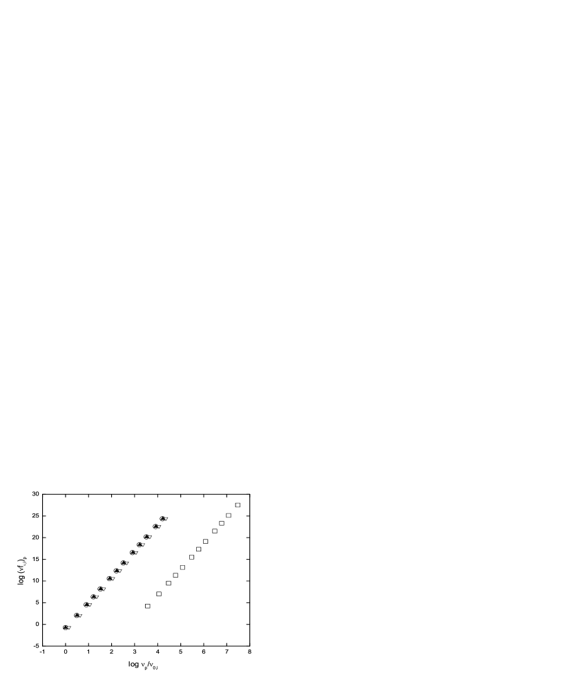
Figure 5: The plots of log$(\nu f_{\nu})_{p}-log\nu_{p}$ for the bremsstrahlung (open circle), Comptonized (open triangle), synchrotron (open square), and the GRB model (filled triangle) radiation, where log$(\nu f_{\nu,i})_{p}$ represents log$(\nu f_{\nu,B})_{p}$, log$(\nu f_{\nu,C})_{p}$, log$(\nu f_{\nu,S})_{p}$ and log$(\nu f_{\nu,G})_{p}$, while log$(\nu_{p}/\nu_{0,i})$ represents log$(\nu_{p}/\nu_{0,B})$, log$(\nu_{p}/\nu_{0,C})$, log$(\nu_{p}/\nu_{0,S})$ and log$(\nu_{p}/\nu_{0,P})$. The data are taken from Tables 1-4.

To obtain an intuitive view of the relation between the two elements, we present Fig. 5. It displays the plots of $\log(\nu f_{\nu})_{p}-\log\nu_{p}$ for the bremsstrahlung, Comptonized, synchrotron, and the GRB model radiations considered above, respectively, where $\nu_{p}$ is scaled respectively to the typical frequencies adopted in Figs. 1–4 and Tables 1–4 for the corresponding models. The figure shows clearly that the two elements are obviously correlated. Indeed, it was discovered that the mean peak energies of gamma-ray burst spectra are correlated with intensity (Mallozzi et al. (1995)).

5 Change of the spectral shape

In this section, we investigate the change of the spectral shape caused by the expansion of fireballs. A direct comparison between the rest frame radiation and the expected observational radiation is made to show the change. This is realized by adjusting the typical frequencies and the magnitudes of the rest frame radiations, which are used for comparison, of the corresponding models so that the values of $(\nu f_{\nu})_{p}$ as well as $\nu_{p}$ for both the compared rest frame spectrum and the expected observational spectrum are the same.

Figure 6: The plot for comparing the shapes of the expected spectrum of a fireball and the corresponding rest frame spectrum in the case of the bremsstrahlung radiation. The solid lines from the bottom to the top stand for the expected spectra corresponding to $\Gamma=$ 2, 5, 10, 100, 1000, and 10000, respectively, while the dotted lines from the bottom to the top are the compared rest frame spectra for the corresponding, from the bottom to the top, expected spectra.

Figure 7: The plot for comparing the shapes of the expected spectrum of a fireball and the corresponding rest frame spectrum in the case of the Comptonized radiation. The symbols are the same as those in Fig. 6.

Figure 8: The plot for comparing the shapes of the expected spectrum of a fireball and the corresponding rest frame spectrum in the case of the synchrotron radiation. The symbols are the same as those in Fig. 6.

Figure 9: The plot for comparing the shapes of the expected spectrum of a fireball and the corresponding rest frame spectrum in the case of the radiation bearing the GRB form. The symbols are the same as those in Fig. 6.

Shown in Figs. 6–9 are the same plots of Figs. 1–4, where the expected observational spectra as well as the corresponding compared rest frame spectra are presented.

These figures show that when the expansion speed is not extremely large (say, $\Gamma\leq 1000$), the expected spectra become slightly widened and are less steep at higher frequency bands for the bremsstrahlung, Comptonized, and synchrotron radiations, and at lower frequency bands for the GRB model radiation. The shapes of the expected spectra are almost the same as the rest frame ones. Therefore, for constant radiations, when a certain form can well describe the observed spectrum at a given observation time, it would also be able to represent the observed spectrum at other observation time. In particular, when we observe a decrease of the temperature (say, $T_{B}$ in the bremsstrahlung or $T_{C}$ in the Comptonized radiation, see Schaefer et al. (1994)), we would expect a decrease of the intensity as well due the decrease of the expansion speed (which causes the observed decrease of the temperature), as long as the radiation is constant.

6 Enhancement of the flux

We note that the expected flux of an expanding fireball would vary with both frequency and the expansion speed. Different from those figures shown in section 3, we present here plots of $\log(\nu f_{\nu})-\log\Gamma$ at some particular frequencies for the radiations considered above, which would plainly show the enhancement of fluxes caused by the expansion of fireballs. They are Figs. 10–13. Figs. 10–12 show that, for constant radiations of the bremsstrahlung, Comptonized, and synchrotron mechanisms, when the expansion speed decreases steadily, fluxes at higher frequencies would decrease very rapidly and later might become undetectable, while those at lower frequencies would also decrease but in a much slow manner. But this phenomenon would be rare because the number of fireballs with the expansion speed that large would be small. From Fig. 13 one finds that, for a constant radiation of the GRB form, when the expansion speed decreases steadily, fluxes at any (lower or higher) frequencies would decrease in almost the same manner.

Figure 10: The plot of log($\nu$f_ν,B) — log$\Gamma$ for the bremsstrahlung radiation at various frequencies [the solid lines from the bottom to the top: log($\nu/\nu_{0,B}$) = –4, –2, 0; the dashed line: log($\nu/\nu_{0,B}$) = 2; the dotted line: log($\nu/\nu_{0,B}$) = 3; the dashed and dotted line: log($\nu/\nu_{0,B}$) = 4; the short and long dashed line: log($\nu/\nu_{0,B}$) = 5].

Figure 11: The plot of log($\nu$f_ν,C) — log$\Gamma$ for the Comptonized radiation at various frequencies [the solid lines from the bottom to the top: log($\nu/\nu_{0,C}$) = –4, –2, 0; the dashed line: log($\nu/\nu_{0,C}$) = 2; the dotted line: log($\nu/\nu_{0,C}$) = 3; the dashed and dotted line: log($\nu/\nu_{0,C}$) = 4; the short and long dashed line: log($\nu/\nu_{0,C}$) = 5].

Figure 12: The plot of log($\nu$f_ν,S) — log$\Gamma$ for the synchrotron radiation at various frequencies [the solid lines from the bottom to the top: log($\nu/\nu_{0,S}$) = 0, 2, 4; the dashed line: log($\nu/\nu_{0,S}$) = 6; the dotted line: log($\nu/\nu_{0,S}$) = 8; the dashed and dotted line: log($\nu/\nu_{0,S}$) = 9; the short and long dashed line: log($\nu/\nu_{0,S}$) = 10].

Figure 13: The plot of log($\nu$f_ν,G) — log$\Gamma$ for the radiation bearing the GRB form at various frequencies [the solid lines from the bottom to the top: log($\nu/\nu_{0,p}$) = –4, –2, 0, 2; the dotted line: log($\nu/\nu_{0,p}$) = 4; the dashed line: log($\nu/\nu_{0,p}$) = 6; the dashed and dotted line: log($\nu/\nu_{0,p}$) = 8].

These figures also show that, the expansion speed plays a very important role in the enhancement of fluxes: when the value of $\Gamma$ becomes 10 times larger, the flux would be several orders of magnitude larger. The expansion speed of fireballs would determine relative magnitudes of their fluxes observed and thus might determine if a gamma-ray source is detectable. Note that $(1+z)^{2}$ is the main factor of the cosmological effect. That suggests that the effect caused by the expansion speed of fireballs is really very large and would be the fundamental factor of the enhancement of the flux of the objects.

7 Conclusions

In this paper, we investigate how the Doppler effect in the fireball framework plays a role on the spectrum of gamma-ray bursts.

We find that the shape of the expected spectrum of an expanding fireball remains almost the same as that of the corresponding rest frame spectrum for constant radiations of the bremsstrahlung, Comptonized, and synchrotron mechanisms as well as for that of the GRB model. However, as the fireball expands, the peak of the spectrum would shift to a higher frequency band and the flux over the entire frequency range would be amplified. The study reveals that the peak flux spectrum $(\nu f_{\nu})_{p}$ and the peak frequency $\nu_{p}$ are obviously correlated, meeting what was discovered recently (Mallozzi et al. (1995)). The expansion speed plays a very important role in the enhancement of fluxes: when the value of $\Gamma$ becomes 10 times larger, the flux would be several orders of magnitude larger. Even the expansion speed is not very large (say $\Gamma=2$), a dim and undetectable X-ray rest frame radiation might become an observable gamma-ray source. The expansion speed of fireballs is a fundamental factor of the enhancement of the flux of GRBs.

The study shows that, for constant radiations of the bremsstrahlung, Comptonized, and synchrotron mechanisms, when the expansion speed decreases steadily, fluxes at higher frequencies would decrease very rapidly and later might become undetectable, while those at lower frequencies would also decrease but in a much slow manner. However, for a constant radiation of the GRB form, when the expansion speed decreases steadily, fluxes at any (lower or higher) frequencies would decrease in almost the same manner.

It is my great pleasure to thank Prof. M. J. Rees for his helpful suggestions and discussion. Parts of this work were done when I visited Institute of Astronomy, University of Cambridge and Astrophysics Research Institute, Liverpool John Moores University. Thanks are also given to these institutes. This work was supported by the Special Funds for Major State Basic Research Projects, National Natural Science Foundation of China.

Appendix A Detailed derivation of the formula

We concern a fireball expanding at a constant velocity $v=\beta c$ (where $\mathbf{c}$ is the speed of light) and adopt a spherical coordinate system with its origin being sited at the center of the fireball and its axis being the line of sight. Consider radiation from the rest frame differential surface, $ds_{0,\theta,\varphi}$, of the fireball at proper time $t_{0,\theta}$, where $\theta$ denotes the angle to the line of sight and $\varphi$ denotes the other angular coordinate of the fireball surface. Let $ds_{\theta,\varphi}$ be the corresponding differential surface resting on the observer framework, coinciding with $ds_{0,\theta,\varphi}$ at $t_{0,\theta}$. Obviously, $ds_{0,\theta,\varphi}$ moves at velocity $v$ relative to $ds_{\theta,\varphi}$.

Let $t_{\theta}$ be the corresponding coordinate time when $ds_{\theta,\varphi}$ coincides with $ds_{0,\theta,\varphi}$ at $t_{0,\theta}$. According to the theory of special relativity, $t_{\theta}$ and $t_{0,\theta}$ are related by

$$t_{\theta}-t_{c}=\Gamma(t_{0,\theta}-t_{0,c}),$$ (25)

where $t_{c}$ and $t_{0,c}$ are constants (here we assign $t_{\theta}=t_{c}$ when $t_{0,\theta}=t_{0,c}$), and $\Gamma$ is the Lorentz factor of the fireball.

The area of $ds_{\theta,\varphi}$ is

$$ds_{\theta,\varphi}=R^{2}(t_{\theta})\sin\theta d\theta d\varphi,$$ (26)

where $R(t_{\theta})$ is the radius of the fireball at $t_{\theta}$. The radius follows

$$R(t_{\theta})=\beta c(t_{\theta}-t_{c})+R_{c},$$ (27)

where $R_{c}$ is the radius at time $t_{\theta}=t_{c}$. As assigned above, $t_{\theta}$ and $t_{0,\theta}$ correspond to the same moment, thus the radius can also be expressed as

$$\ R_{0}(t_{0,\theta})=R[t_{\theta}(t_{0,\theta})]=\Gamma\beta c(t_{0,\theta}-t_{0,c})+R_{c},$$ (28)

where equation (A1) is applied.

Let us consider an observation within the small intervals $t$ — $t+dt$ and $\nu$ — $\nu+d\nu$ carried out by an observer with a detector $\triangle s_{ob}$ at a distance $D$ ($D$ is the distance between the observer and the center of the fireball), where $D\gg R(t_{\theta})$. Suppose radiation from $ds_{0,\theta,\varphi}$ arriving the observer within the above observation intervals is emitted within the proper time interval $t_{0,\theta}$ — $t_{0,\theta}+dt_{0,\theta}$ and the rest frame frequency interval $\nu_{0,\theta}$ — $\nu_{0,\theta}+d\nu_{0,\theta}$. According to the Doppler effect, $\nu$ and $\nu_{0,\theta}$ are related by

$$\nu=\frac{\nu_{0,\theta}}{\Gamma(1-\beta\cos\theta)}.$$ (29)

Considering the travelling of light from the fireball to the observer, one would come to

$$c(t-t_{\theta})=D-R(t_{\theta})\cos\theta,$$ (30)

(note that the cosmological effect is ignored). Combining (A1), (A3) and (A6) yields

$$t_{\theta}=\frac{t-D/c+(R_{c}/c-\beta t_{c})\cos\theta}{1-\beta\cos\theta}$$ (31)

and

$$t_{0,\theta}=\frac{t-t_{c}-D/c+(R_{c}/c)\cos\theta}{\Gamma(1-\beta\cos\theta)}+t_{0,c}.$$ (32)

The radius of the fireball then can be written as

$$R[t_{\theta}(t)]=R_{0}[t_{0,\theta}(t)]=\frac{\widetilde{R}(t)}{1-\beta\cos\theta},$$ (33)

with

$$\widetilde{R}(t)=\beta[c(t-t_{c})-D]+R_{c}.$$ (34)

Suppose photons, which are emitted from $ds_{0,\theta,\varphi}$ within proper time interval $t_{0,\theta}$ — $t_{0,\theta}+dt_{0,\theta}$ and then reach the observer within $t$ — $t+dt$, pass through $ds_{\theta,\varphi}$ within coordinate time interval $t_{\theta}$ — $t_{\theta}+dt_{\theta,s}$. Since both $ds_{\theta,\varphi}$ and the observer rest on the same framework, it would be held that $dt_{\theta,s}=dt$ (when the cosmological effect is ignored). Of course, the frequency interval for the photons measured by both $ds_{\theta,\varphi}$ and the observer must be the same: $\nu$ — $\nu+d\nu$. Suppose the radiation concerned is independent of directions. Then in the view of $ds_{\theta,\varphi}$ (which is also the view of the observer), the amount of energy emitted from $ds_{0,\theta,\varphi}$ within $t_{0,\theta}$ — $t_{0,\theta}+dt_{0,\theta}$ and $\nu_{0,\theta}$ — $\nu_{0,\theta}+d\nu_{0,\theta}$ (which would pass through $ds_{\theta,\varphi}$ within $t_{\theta}$ — $t_{\theta}+dt$ and be measured within $\nu$ — $\nu+d\nu$) towards the observer would be

$$dE_{\theta,\varphi}=I_{\nu}(t_{\theta},\nu)\cos\theta ds_{\theta,\varphi}d\omega d\nu dt,$$ (35)

where $I_{\nu}(t_{\theta},\nu)$ is the intensity of radiation measured by $ds_{\theta,\varphi}$ or by the observer and $d\omega$ is the solid angle of $\triangle s_{ob}$ with respect to the fireball, which is

$$d\omega=\frac{\triangle s_{ob}}{D^{2}}.$$ (36)

(It is clear that any elements of emission from the fireball are independent of $\varphi$ due to the symmetric nature of the object.) Thus,

$$dE_{\theta,\varphi}=\frac{\triangle s_{ob}d\nu dtR^{2}(t_{\theta})I_{\nu}(t_{\theta},\nu)\cos\theta\sin\theta d\theta d\varphi}{D^{2}},$$ (37)

where (A2) and (A12) are applied.

The total amount of energy emitted from the whole fireball surface detected by the observer within the above observation intervals is an integral of $dE_{\theta,\varphi}$ over that area, which is

$$dE=\frac{2\pi\triangle s_{ob}d\nu dt}{D^{2}}\int_{\theta_{\min}}^{\theta_{\max}}R^{2}(t_{\theta})I_{\nu}(t_{\theta},\nu)\cos\theta\sin\theta d\theta,$$ (38)

where $\theta_{\min}$ and $\theta_{\max}$ are determined by the fireball surface itself together with the emitted ranges of $t_{0,\theta}$ and $\nu_{0,\theta}$. Thus, the expected flux would be

$$f_{\nu}(t)=\frac{2\pi}{D^{2}}\int_{\theta_{\min}}^{\theta_{\max}}R^{2}(t_{\theta})I_{\nu}(t_{\theta},\nu)\cos\theta\sin\theta d\theta.$$ (39)

It is well known that the observer frame intensity $I_{\nu}(t_{\theta},\nu)$ is related to the rest frame intensity $I_{0,\nu}(t_{0,\theta},\nu_{0,\theta})$ by

$$I_{\nu}(t_{\theta},\nu)=(\frac{\nu}{\nu_{0,\theta}})^{3}I_{0,\nu}(t_{0,\theta},\nu_{0,\theta}).$$ (40)

The flux then can be written as

$$f_{\nu}(t)=\frac{2\pi}{D^{2}\Gamma^{3}}\int_{\theta_{\min}}^{\theta_{\max}}\frac{R_{0}^{2}(t_{0,\theta})I_{0,\nu}(t_{0,\theta},\nu_{0,\theta})\cos\theta\sin\theta}{(1-\beta cos\theta)^{3}}d\theta,$$ (41)

where (A4) and (A5) are applied.

Now let us find out how $\theta_{\min}$ and $\theta_{\max}$ are determined. We are aware that the range of $\theta$ of the visible fireball surface is

$$0\leq\theta\leq\pi/2.$$ (42)

Within this range, suppose the emitted ranges of $t_{0,\theta}$ and $\nu_{0,\theta}$ constrain $\theta$ by

$$\theta_{t,\min}\leq\theta\leq\theta_{t,\max}$$ (43)

and

$$\theta_{\nu,\min}\leq\theta\leq\theta_{\nu,\max},$$ (44)

respectively. Then when the following condition

$$\max\{\theta_{t,\min},\theta_{\nu,\min}\}<\min\{\theta_{t,\max},\theta_{\nu,\max}\}$$ (45)

is satisfied, $\theta_{\min}$ and $\theta_{\max}$ would be obtained by

$$\theta_{\min}=\max\{\theta_{t,\min},\theta_{\nu,\min}\}$$ (46)

and

$$\theta_{\max}=\min\{\theta_{t,\max},\theta_{\nu,\max}\},$$ (47)

respectively.

Let the emitted ranges of $t_{0,\theta}$ and $\nu_{0,\theta}$ be

$$t_{0,\min}\leq t_{0,\theta}\leq t_{0,\max}$$ (48)

and

$$\nu_{0,\min}\leq\nu_{0,\theta}\leq\nu_{0,\max},$$ (49)

respectively. From (A8) and (A24) one gets

$$\theta_{t,\min}=\cos^{-1}\left(\min\{1,\frac{\Gamma c(t_{0,\max}-t_{0,c})+D-c(t-t_{c})}{\Gamma\beta c(t_{0,\max}-t_{0,c})+R_{c}}\}\right)$$

(50)

and

$$\theta_{t,\max}=\cos^{-1}\left(\max\{0,\frac{\Gamma c(t_{0,\min}-t_{0,c})+D-c(t-t_{c})}{\Gamma\beta c(t_{0,\min}-t_{0,c})+R_{c}}\}\right)$$

(51)

For $\beta>0$, one can obtain the following from (A5) and (A25):

$$\theta_{\nu,\min}=\cos^{-1}\left(\min\{1,\frac{1}{\beta}(1-\frac{\nu_{0,\min}}{\Gamma\nu})\}\right)$$

(52)

$$\theta_{\nu,\max}=\cos^{-1}\left(\max\{0,\frac{1}{\beta}(1-\frac{\nu_{0,\max}}{\Gamma\nu})\}\right)$$

(53)

Appendix B Condition for $\theta_{t,\min}=0$ and $\theta_{t,\max}=\pi/2$

Here we show the conditions for retaining $\theta_{t,\min}=0$ and $\theta_{t,\max}=\pi/2$.

Since $R(t_{\theta})>0$, from (A4) and (A8) we find that

$$\frac{\beta c(t-t_{c})-\beta D+R_{c}}{\Gamma\beta c(1-\beta\cos\theta)}>0.$$ (54)

Then from (A8) we obtain

$$\frac{dt_{0,\theta}}{d\cos\theta}=\frac{\beta c(t-t_{c})-\beta D+R_{c}}{\Gamma c(1-\beta\cos\theta)^{2}}>0.$$ (55)

It suggests that

$$t_{0,\pi/2}\leq t_{0,\theta}\leq t_{0,0}.$$ (56)

From (A24) and (B3) one finds that, when

$$t_{0,\min}\leq t_{0,\pi/2}$$ (57)

and

$$t_{0,\max}\geq t_{0,0},$$ (58)

one would get $\theta_{t,\min}=0$ and $\theta_{t,\max}=\pi/2$. Applying (A8) leads to

$$t_{0,\min}\leq\frac{c(t-t_{c})-D}{\Gamma c}+t_{0,c}$$ (59)

and

$$t_{0,\max}\geq\frac{c(t-t_{c})-D+R_{c}}{\Gamma c(1-\beta)}+t_{0,c}.$$ (60)

References

• Band et al. (1993) Band, D., et al. 1993, ApJ, 413, 281
• Brainerd et al. (1998) Brainerd, J. J., et al. 1998, ApJ, 501, 325
• Ford et al. (1995) Ford, L. A., et al. 1995, ApJ, 439, 307
• Goodman (1986) Goodman, J. 1986, ApJ, 308, L47
• Katz (1994) Katz, J. I. 1994, ApJ, 422, 248
• Klebesadel et al. (1973) Klebesadel, R., Strong, I., & Olson, R. 1973, ApJ, 182, L85
• Krolik & Pier (1991) Krolik, J. H., & Pier, E. A. 1991, ApJ, 373, 277
• Liang et al. (1983) Liang, E. P., Ternigan, T. E., & Rodrigues, R. 1983, ApJ, 271, 766
• Mallozzi et al. (1995) Mallozzi, R. S., et al. 1995, ApJ, 454, 597
• Meszaros & Rees (1993) Meszaros, P., & Rees, M. J. 1993, ApJ, 405, 278
• Meszaros & Rees (1994) Meszaros, P., & Rees, M. J. 1994, MNRAS, 269, L41
• Meszaros & Rees (1998) Meszaros, P., & Rees, M. J. 1998, ApJ, 502, L105
• Paczynski (1986) Paczynski, B. 1986, ApJ, 308, L43
• Paczynski & Xu (1994) Paczynski, B., & Xu, G. 1994, ApJ, 427, 708
• Preece et al. (1998) Preece, R. D., et al. 1998, ApJ, 496, 849
• Preece et al. (2000) Preece, R. D., et al. 2000, ApJS, 126, 19
• Ramaty & Meszaros (1981) Ramaty, R., & Meszaros, P. 1981, ApJ, 250, 384
• Rees & Meszaros (1992) Rees, M. J., & Meszaros, P. 1992, MNRAS, 258, 41p
• Rees & Meszaros (1994) Rees, M. J., & Meszaros, P. 1994, ApJ, 430, L93
• Sari et al. (1996) Sari, R., Narayan, R., & Piran, T. 1996, ApJ, 473, 204
• Schaefer et al. (1994) Schaefer, B. E., et al. 1994, ApJS, 92, 285