Einstein-Rosen Bridges and the Characteristic Properties
of Gravitational Lensing by Them.

A.A. Shatskiy

Abstract

It is shown that Einstein-Rosen bridges (wormholes) hypothetical objects that topologically connect separate locations in the Universe can be static solutions of the Einstein equations. The corresponding equations for bridges are reduced to a form convenient for their analysis and numerical solution. The matter forming the bridge must have a sufficiently hard and anisotropic equation of state. Our results are compared with a previously known analytic solution for a bridge, which is a special case of the general solution in the framework of general relativity. The deflection of photons by the bridge (gravitational lensing) is studied.

1 INTRODUCTION

In recent years, there have been an increasing number of publications in relativistic astrophysics devoted to so-called ”wormholes”. Another term for these objects proposed by Einstein and Rosen [1] in 1935 is ”bridge”.

There are several different definitions of bridges, depending on the presence or absence of event horizons in them. A common feature of all these definitions is that the bridge connects two asymptotically at spatial regions. The location of such a connection is the bridge, and its central part is called the bridge’s throat (Fig.1). Space-time is strongly curved near the throat. We shall consider here only traversable Lorentzian wormholes, i.e. those through which physical bodies can pass. Consequently there must be no event horizons in such bridges.

As was proved long time ago [2], bridges can be constructed in general relativity only from matter with exotic equations of state (for more details, see below). Such matter has not been found in the Universe thus far. Therefore, bridge solutions were first sought in alternative theories of gravity such as the Brans-Dicke theory and theories involving quantum-gravitational effects.

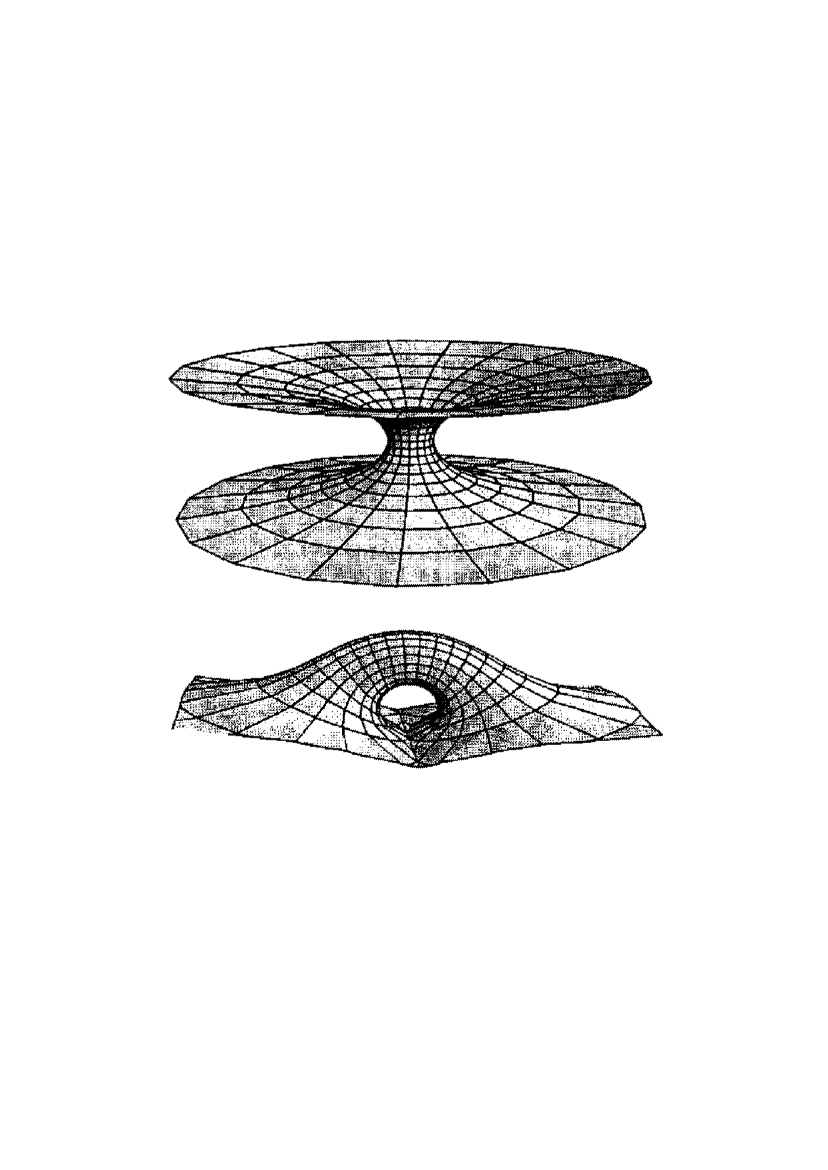
Figure 1: Spherically symmetric bridge connecting two parts of the Universe (top panel) and a non-spherically symmetric ”door-handle” bridge connecting two distant parts of the same Universe (bottom panel).

Despite all these problems, bridges have been attracting increasing interest. This is due in our view to the following four factors.

(1) The existence of dark matter which may obey an unusual equation of state.

(2) Bridges could be real and observable astrophysical objects, such as black holes, whose existence was likewise long rejected by many scientists.

(3) Huge progress in computer modeling of multidimensional structures has made it possible to solve numerically many problems in relativistic astrophysics. Most of these problems cannot be solved using analytic methods because of their extreme complexity.

(4) There have been serious discussions of solutions of the equations of general relativity containing time loops, which imply the existence of time machines (see, for example, [3]).

We shall not discuss here speculations based on

the fourth factor. Our aim is to present the basic ideas of the physics of bridges and their direct relationship to the theory of gravity and black-hole physics. The bridges will be considered in a general-relativitistic treatment.

2 SPHERICALLY SYMMETRIC SYSTEMS

Analytic studies can be carried out most easily for spherically symmetric systems, for which all quantities depend only on time and radius. The form of the solutions of the equations of general relativity does not depend only on the symmetry of the system. Nevertheless, even in cases with the simplest central symmetry exact solutions have been obtained for only a few cases. These are the case of dust matter (the pressure is equal to zero) and of the vacuum condensate (the pressure is the negative of the energy density). It is assumed in inflationary cosmological models that this latter equation of state was dominant for matter in the initial stage of development of the Universe after the Big Bang (a de Sitter universe) [4].

In more realistic cases, for example, when the pressure is proportional to the energy density with a positive coefficient (in particular an ideal photon gas is described by the equation of state with a coefficient of $1/3$ ), we have no exact solutions, and only numerical solutions are available. Moreover even for the simplest models in which all quantities depend only on radius, exact solutions have been found for only a few cases.

An illustrative example of static solutions are ordinary stars and planets. However in reality they obey a fairly sophisticated nonlinear equation of state. As a result, only numerical solutions can be obtained for these objects in a general-relativitistic treatment. The spherically symmetric metric in general relativity can be written:

$$ds^{2}=\exp(\nu)\,dt^{2}-\exp({\rm\lambda})\,dr^{2}-r^{2}\,d\Omega^{2}$$ (1)

Here, $\nu=2\varphi$ is twice the red (or violet) shift, $\varphi=(\Delta f)/f$, $f$ is the photon frequency at infinity near the source, and $d\Omega^{2}$ is an element of solid angle. In the general case, the energy momentum tensor in commoving matter with a spherically symmetric distribution has the form :

$$4\pi T^{0}_{0}=\varepsilon\,,\quad 4\pi T^{1}_{1}=-P_{\parallel}\,,\quad 4\pi T_{2}^{2}=4\pi T_{3}^{3}=-P_{\perp}\,.$$ (2)

It is convenient to describe motion in the spherically symmetric field using the function $V^{2}$ which is the square of the invariant velocity of the particle with respect to the spheres $r=const$:

$$V^{2}=\left({dr\over dt}\right)^{2}\,e^{{\rm\lambda}-\nu},\,.$$ (3)

A more detailed definition of $V^{2}$ is presented in [5]. When a falling particle reaches an event horizon the velocity $V$ reaches unity. The corresponding element of the interval $ds$ is zero so that $V^{2}$ is an invariant at the horizon; i.e. it does not depend on the choice of coordinate system. In the case of free fall (along geodetic trajectories), $V^{2}=1-\exp(\nu)\cdot const$. In the nonrelativistic limit, the definition of $V^{2}$ coincides with the usual definition of the velocity.

For the collapse of dust matter or a Schwarzschild black hole $(P_{\parallel}=P_{\perp}=0)$, we obtain

$$\begin{array}[]{lll}ds^{2}=(1-r_{g}/r)^{+1}\,dt^{2}-(1-r_{g}/r)^{-1}\,dr^{2}-r^{2}\,d\Omega^{2}\,,\\ \\ V^{2}=\left[(R_{0}/r)-1\right]/\left[(R_{0}/r_{g})-1\right]\,.\end{array}$$ (4)

Here and below $R_{0}$ is the initial value of the $r$ coordinate for the falling particle and the event horizon is defined by $V=1$ .

For an inflating de Sitter universe $(P_{\parallel}=P_{\perp}=-\varepsilon)$, we obtain

$$\begin{array}[]{lll}ds^{2}=(1-r^{2}/a^{2}_{{}_{H}})^{+1}\,dt^{2}-(1-r^{2}/a^{2}_{{}_{H}})^{-1}\,dr^{2}-r^{2}\,d\Omega^{2}\,,\\ \\ V^{2}=\left[(r/R_{0})^{2}-1\right]/\left[(a_{{}_{H}}/R_{0})^{2}-1\right]\,.\end{array}$$ (5)

Here, $H\equiv 1/a$, $H$ is the Hubble constant.

3 BRIDGES

The relation between the circumference of a circle and its radius is violated in curved space. Therefore, to avoid misunderstanding, let us introduce the following new coordinates. Let us choose some point in space as a central point. Next we draw rays from this point in all directions. Distance along the rays will be measured by the coordinate $l$ and distance in the perpendicular direction by the coordinate $r$ . Therefore, the circumference will be (by definition) $2\pi r$ while the distance from the center of the circle to its boundary will be (by definition) $l$. In such coordinates, expression (1) for a static case takes the form

$$ds^{2}=\exp(2\phi)\,dt^{2}-dl^{2}-r^{2}\,d\Omega^{2}$$ (6)

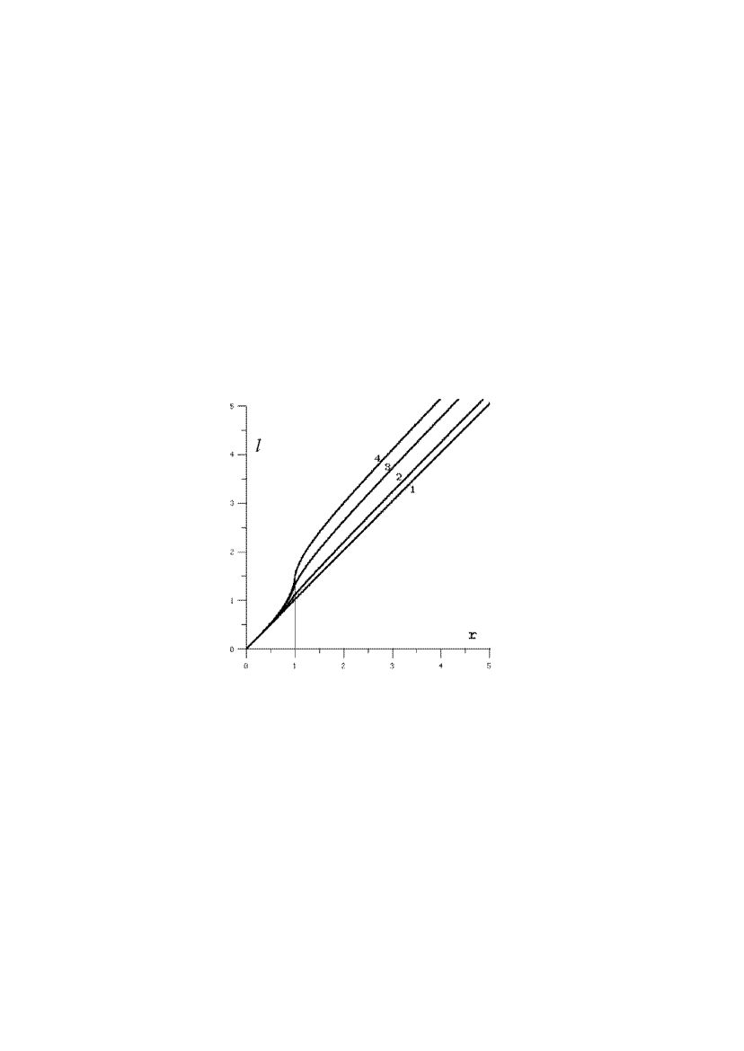
Figure 2: The dependence of $l$ on $r$ for various values of the Newtonian potential $\varphi_{g}$ at the surface of a body $(r=1)$: (1) $\varphi_{g}=0.1$ nearly coincident with the straight line $l=r$ corresponding to $\varphi_{g}=0$, (2) $\varphi_{g}=0.5$, (3) $\varphi_{g}=0.9$ and (4) $\varphi_{g}=0.99$.

In a curved space $r\neq l$. To illustrate this fact let us put a small mass (for example, a planet such as the Earth) at the center of the system. Here, ”small mass” implies a body whose Newtonian gravitational potential at its surface is much less than the square of the speed of light. For the Earth, this potential is $\varphi_{g}\sim 10^{-9}$; for the Sun $\varphi_{g}\sim 10^{-5}$ and for a pulsar $\varphi_{g}\sim 0.5$. The dependence of $l$ on $r$ is illustrated by the plots in Fig.2. This curving the space-time by gravitating matter was predicted by Einstein and subsequently confirmed by numerous experiments.

As the central body becomes heavier it curves space more strongly and stretches it along the radii. When a certain limit is achieved the space is curved so strongly that a black hole is formed. What are the limiting objects just before the formation of black holes, and are black holes always formed?

One well-known limit is a neutron star (pulsar), whose mass is of the order of a solar mass and whose radius is about ten kilometers; the average density of matter in the neutron star is approximately equal to the density of an atomic nucleus $\sim 10^{13}g/cm^{3}$.

The above-mentioned curvature of the space is negligible for normal stars and planets, and is important only for neutron stars (see curve 2 in Fig.2). The limiting curvature occurs when the inclination of the curve $l(r)$ with respect to the $r$ axis increases from $45^{\circ}$ (the uncurved geometry) to $90^{\circ}$ (the most curved geometry). In this case, we obtain a zero increment in $r$ for a nonzero increment in $l$. In Fig.2 curve 4 with $\varphi_{g}=0.99$ is closest to this situation (as follows from calculations this limit is not actually reached: the star collapses before this occurs when $\varphi_{g}\sim 0.5$). After the collapse of a star to a black hole, $l$ becomes imaginary after it passes the singularity indicated above. This is not a physical but a coordinate singularity at the black-hole event horizon, which can be avoided by an appropriate coordinate transformation. The condition $V=1$ can serve as the invariant definition of the horizon [see (3)].

There is also an alternative to the curving of physical space by a black hole. Above a decrease in the $l$ was accompanied by a decrease in $r$. If there is a black hole at the center of the system, the coordinate $l$ becomes imaginary at its event horizon. However there are static solutions in general relativity in which, after passage of the singularity $r$ again begins to increase as $l$ is decreased. Such solutions can correspond to bridges.

Let us present here the definition of a bridge that has been adopted in a number of studies (for example, [6]):

(1) A bridge must have a region where $r$ reaches a local minimum, $r_{0}$. This region is called the throat of the bridge, and $r_{0}$ the throat radius (Fig.1). This is the main difference between a bridge and any other body.

(2) There must be no event horizons in the bridge; i.e., bodies falling into the bridge must not reach the speed of light $(V<1)$ and consequently they should be observable for an external observer.

(3) Bodies can pass through the bridge throat in both directions.

Geometry can be different on the opposite sides of the bridge throat. We shall consider from here on only spherically symmetric static solutions for bridges obeying the equation of state

$$P_{\parallel}={w_{{}_{\parallel}}}\varepsilon\,,\quad P_{\perp}={w_{{}_{\perp}}}\varepsilon\,.$$ (7)

Here, $w_{\parallel}$ and $w_{\perp}$ are constant parameters, and the energy density must not be negative. Such matter is, of course, idealized, but it enables us to study analytically many important features of bridges.

The matter forming such bridges should have exotic properties, since the allowed range of $w_{\parallel}$ and $w_{\perp}$ is restricted by the inequality (see Appendix 8.1)

$$\varepsilon>0\,,\qquad-2{w_{{}_{\perp}}}<{w_{{}_{\parallel}}}<-1\,.$$ (8)

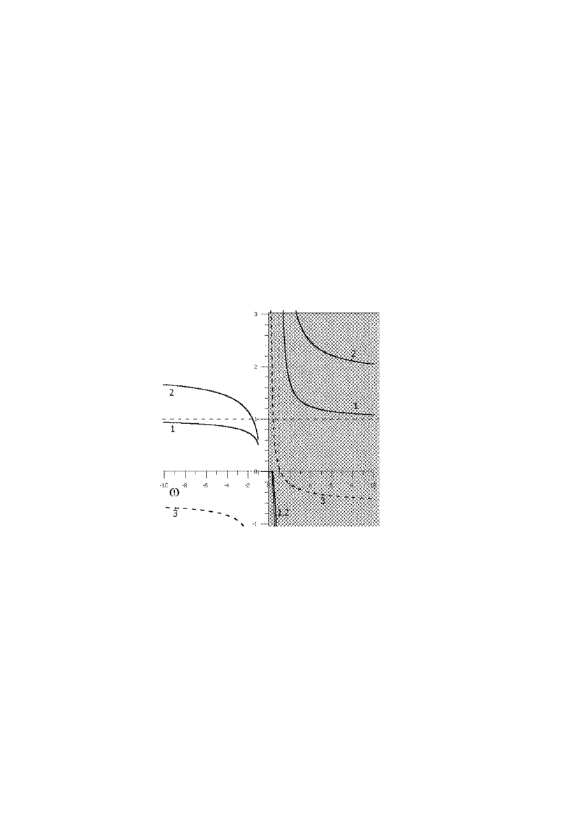
Figure 3: Dependence of the following quantities for bridges on the equation of state (namely on $w=w_{\parallel}=-w_{\perp}$): (1) $r_{0}/r_{g}$, (2) $r_{l}/r_{g}$, (3) $\varphi_{max}$. The left-hand (unshaded) side of the plots corresponds to the physical region $\varepsilon>0$ and the right-hand (shaded) side to the unphysical region $\varepsilon<0$.

We can see that, in order for a bridge to exist, the signs of $w_{\parallel}$ and $w_{\perp}$ must be opposite. Therefore, the equation of state must be substantially hard and anisotropic.

The mass $m$ and gravitational radius $r_{g}$ of a bridge are defined in the same way as for any other body via the field asymptotics at in infinity:

$$\lim\limits_{r\to\infty}\exp(-\lambda)=1-r_{g}/r\,,\quad m=r_{g}/2\,.$$ (9)

In addition to its mass, a bridge is characterized by two dimensions: its length and width. The bridge width can be identified with the size of its throat $r_{0}$. The bridge length can be reasonably related to the physical characteristics of a body passing through the bridge, for example, the change in the red (or violet) shift of the signal received from this body. Therefore, let us define the bridge length $r_{l}$ to be the distance between the points at which the red (or violet) shift from a body at rest is half its maximum value. In the spherically symmetric case, the ratios $r_{0}/r_{g}$ and $r_{l}/r_{g}$ depend only on the equation of state of the bridge. Figure 3 presents the dependences of the ratios $r_{0}/r_{g}$ and $r_{l}/r_{g}$ on $w=w_{\parallel}=-w_{\perp}$ obtained numerically (see Appendix 8.1). The first diagram in this figure clearly shows why bridges exist only when $w<-1$: the function $r_{0}/r_{g}$ tends to zero as $w\to-1$. Therefore, the radius of the throat decreases to zero, and passage to another part of the Universe is no longer possible.

4 FORMATION AND EXISTENCE OF BRIDGES

The question of the formation (and, in general, the existence) of bridges remain open and two scenarios are possible.

1. The trivial scenario: bridge were formed during the birth of our part of the Universe and still exist, preserving the global topology (geometry) of the Universe. This is the only way to form bridges connecting two different parts of our Universe (like a door handle), since the modern geometrical theorems of general relativity forbid the disruption of such a topology [7]. We cannot currently answer the question of how this topology was created since Einsteinian gravitational theory cannot be applied to the birth of the Universe (quantum gravity which remains incompletely developed must be used).

2. The dynamic scenario: bridges could be formed instead of black holes as ”branches ”in the process of evolution of the Universe. This process of detachment is drawn schematically in Fig.4. First, the matter (accumulated due to self-gravity) curves space. Next, the amount of matter becomes sufficient to curve the geometry to the limiting value at some radius (Fig.2). The matter then begins to inflate the space behind this radius, similar to the inflation of space by the vacuum condensate in the observed expanding Universe (as a consequence of negative pressure). There must be no event horizons anywhere. The resulting branch evolves by itself, expands, and forms a new part of the Universe, connected to our part of the Universe by the throat of the bridge.

Figure 4: Probable dependence of $r$ on $l$ in a bridge during its detachment. The numbers 1 to 5 correspond to successive times in the bridge’s evolution.

5 OBSERVATION OF BRIDGES

The simplest way to detect a bridge is to observe some objects (e.g. stars) through its throat. If the geometry of the Universe is different on the opposite sides of the throat (see Appendix 8.2), the rate of flow of time will also be different. As a result, photons passing the bridge’s throat will experience a red (or violet) shift. An important problem with this method is to discriminate such shifts from Doppler shifts due to the source motion.

Another method is based on the idea that the photons in light signals passing through the throat of a bridge should experience a deflection; i.e., they should undergo lensing by the curved geometry of the space (see, for example,[8]). Let us define the impact parameter $h$ for a photon deflected by a bridge to be $h=L/E$ the ratio of the angular momentum and energy of the photon at infinity.

There are two type of lensing (see Appendix 8.3).

1. The photon does not pass through the throat, and so always remains in the same part of the Universe. This situation takes place for photons that have sufficiently large impact parameters (in comparison with the throat radius) and are deflected by the gravitational lens.

2. The photon passes through the throat to another part of the Universe. This situation takes place for photons having sufficiently small impact parameters (compared to the throat radius). One characteristic feature of this effect is that the deflection of the photons is given by the formula for a thin converging lens whose focal distance is approximately equal to the throat radius. In the case of other gravitating centers, these photons would be absorbed by the surface of the body.

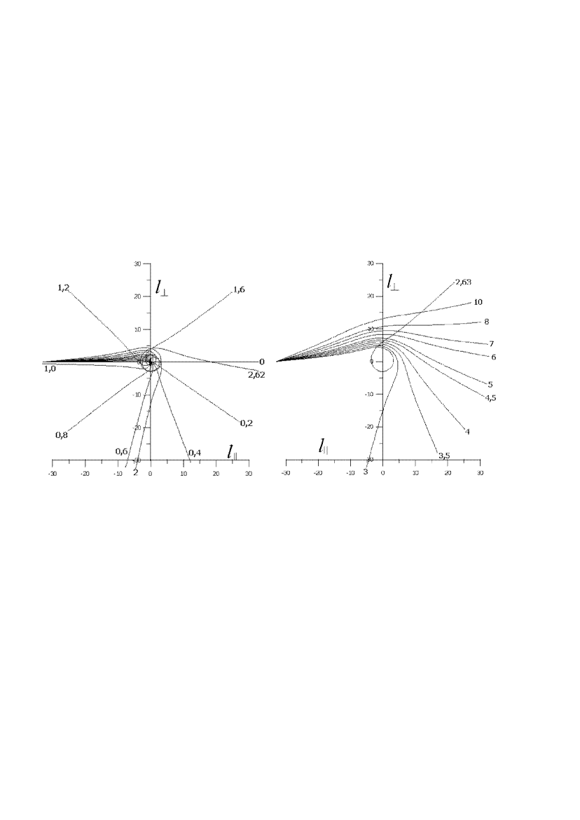
Figure 5: Deflection of photons by a bridge with $w=-2$. The trajectories of photons deflected through an angle $\Delta\varphi$ from the initial direction are plotted. The trajectories start at $l=-32r_{0}$, $\varphi=-\pi$. Trajectories passing through the throat at small impact parameters ($h<h_{cr}\approx 2.621r_{0}$) and terminating at $l\to+\infty$ are shown in the left-hand panel. Trajectories not passing through the throat ($h>h_{cr}$) and terminating at $l\to-\infty$ are shown in the right-hand panel. The numbers near the ends of the curves indicate the impact parameters (in units of $r_{0}$). The coordinates $l_{\parallel}$, $l_{\perp}$ denote the equatorial plane of the photon scattering ($l_{\parallel}=+|l|\cos\varphi$, $l_{\perp}=-|l|\sin\varphi$).

The calculated photon trajectories for a bridge with $w=-2$ are presented in Fig.5. If the impact parameter is close to the critical value $h_{cr}$, the photons can be deflected through large angles (greater than $2\pi$) by the bridge. Note that photons passing through the throat inevitably intersect the center of the bridge; i.e., the point $l=0$. There is no singularity at this point, since the value $l=0$ corresponds to a sphere of finite radius $r_{0}$.

Since the photon impact parameter does not change and corresponds to a location in the bridge ’s throat (relative to its center) from which we can observe the light of a star from another part of the Universe, the impact parameter can be used to determine the deflection angle of the photon on its way to the observer. In fact this is a method to determine the coordinates of stars in that part of the Universe.

6 DISCUSSION

Not only photons, but also physical bodies can pass through a bridge. The main obstacles to this are tidal forces, which disrupt bodies inside black holes and in the orbits of compact stars (such as neutron stars). The tidal forces depend on the curvature of space and the size of the body. Therefore, they coincide to order of magnitude with the corresponding forces in black holes of the same mass. The tidal forces affecting a body of mass $\mu$ and size $d$ are proportional to the derivative of the gravitational forces. For black holes, the tidal forces are equal to $\mu c^{2}d/r^{2}_{g}$ at the event horizon. To order of magnitude, the same forces should act in bridges. If a bridge possesses a sufficiently large mass, then not only macroscopic objects, but also stars, such as the Sun can pass through its throat without disruption. This should be the case for bridges with masses of a few billion solar masses (as in some quasars). A person would not feel the passage through such a bridge, because the tidal forces would be extremely small.

7 CONCLUSIONS

Our main conclusion is that bridges can be real objects, which are described by Einstein gravitational theory in a self-consistent way and can be distinguished from other celestial bodies by observations. The equation of state of the matter in traversable bridges described by general relativity must be substantially hard and anisotropic [see (8)]. Gravitational lensing by bridges is fundamentally different from lensing by other bodies, and precisely these differences can be used to identify bridges and study their properties (as well as the properties of the part of the Universe on the opposite side of the bridge).

ACKNOWLEDGEMENTS

I am grateful to I.D. Novikov and N.S. Kardashev for their help and participation in my preparation of this article. This work was supported by the Program ”Non stationary Phenomena in Astronomy”, the Program of Support for Leading Scientific Schools (project N Sh-1653-2003.2), and the Russian Foundation for Basic Research (project codes 01-02-16812, 01-02-17829, and 00-15-96698).

8 Appendices

8.1 NUMERICAL SOLUTION

The Einstein equations corresponding to (6) and (7) are [9]:

$$2\varepsilon r^{2}=-2r^{\prime\prime}r+(1-{r^{\prime}}^{2}),$$ (10)

$$2{w_{{}_{\parallel}}}\varepsilon r^{2}=2r\phi^{\prime}r^{\prime}-(1-{r^{\prime}}^{2}),$$ (11)

$$2{w_{{}_{\perp}}}\varepsilon=\phi^{\prime\prime}+{\phi^{\prime}}^{2}+(\phi^{\prime}r^{\prime}+r^{\prime\prime})/r$$ (12)

These equations lead to the following expression (which can be derived most easily from the equality $T^{k}_{l;k}\equiv 0$:

$${w_{{}_{\parallel}}}(\ln\varepsilon)^{\prime}=({w_{{}_{\perp}}}-{w_{{}_{\parallel}}})(\ln r^{2})^{\prime}-(1+{w_{{}_{\parallel}}})\phi^{\prime}\,.$$ (13)

Here, a prime denotes a derivative with respect to $l$ which is related to $r$ as

$$dl=\pm\sqrt{\exp({\rm\lambda})}\,dr\,,\quad l(r)=\pm\int\limits_{r_{0}}^{r}\sqrt{\exp({\rm\lambda})}\,dr\,,\quad r(l)=r_{0}\pm\int\limits_{0}^{l}\sqrt{\exp(-{\rm\lambda})}\,dl\,.$$ (14)

Here and below the upper and lower signs correspond to positive and negative values of $l$ respectively. The new constant $r_{0}$ appearing here is defined as the minimum of the function $r(l)$: $r(0)\equiv 0$. Let us introduce the new functions

$$a(l)\equiv r(1-e^{\nu})\,,\quad b(l)\equiv r_{0}+\int\limits_{0}^{l}2\varepsilon r^{2}r^{\prime}\,dl\,,$$ (15)

in which case (10) can be rewritten

$$b^{\prime}\equiv 2\varepsilon r^{2}r^{\prime}=\left[r(1-{r^{\prime}}^{2})\right]^{\prime}$$ (16)

The definitions (14) can be rewritten

$$(r^{\prime})^{2}=\exp(-{\rm\lambda})=1-b/r\,,\quad l=\pm\int\limits_{r_{0}}^{r}\left(1-b/r\right)^{-1/2}\,dr\,.$$ (17)

Consequently the metric (6) will take the form

$$ds^{2}=(1-a/r)\,dt^{2}-(1-b/r)^{-1}\,dr^{2}-r^{2}\,d\Omega^{2}\,.$$ (18)

Equation (11) can be rewritten

$${w_{{}_{\parallel}}}b^{\prime}\equiv 2{w_{{}_{\parallel}}}\varepsilon r^{2}r^{\prime}=2(r-b)\phi^{\prime}-r^{\prime}b/r\,.$$ (19)

In order for the quantities $a$ and $b$ (corresponding to twice the mass of the system) to be limited, the energy density $\varepsilon(r)$ must tend to zero at infinity faster than $const/r^{3}$. The left-hand side of (19) then tends to zero as $r\to\infty$ faster than the right-hand side, and can, therefore, be neglected. In this limit, $\varphi^{\prime}\to ar^{\prime}/(2r^{2})$. Consequently $a$ and $b$ tend to the same limit, which is twice the mass of the system or its gravitational radius:

$$\lim_{r\to\infty}a=\lim_{r\to\infty}b=2m=r_{g}\,.$$ (20)

Since $b(l=0)=b_{0}=r_{0}$ and $\lim_{r\to r_{0}}(r^{\prime})\propto\sqrt{r-b}$ Eq. (19) gives

$$\varepsilon_{0}=-{1\over 2{w_{{}_{\parallel}}}r_{0}^{2}}\,.$$ (21)

Further we can exclude the variable $l$ from (13), (15), and (19) by substituting $r$. Using the new variables

$$x=r/r_{0}\,,\quad y=b/b_{0}\,,\quad\xi=\varepsilon/\varepsilon_{0}\,,$$ (22)

the resulting equations can be reduced to the integral form

$$y(x)=1-{1\over{w_{{}_{\parallel}}}}\int\limits_{1}^{x}\xi x^{2}\,dx\,,$$ (23)

$$\xi^{\prime}(x)=\xi\left[({{w_{{}_{\perp}}}\over{w_{{}_{\parallel}}}}-1){2\over x}+{1\over 2}({1\over{w_{{}_{\parallel}}}}+1){\xi x-y/x^{2}\over 1-y/x}\right]\,,$$ (24)

$$\xi(x)=1+\int\limits_{1}^{x}\xi^{\prime}\,dx\,,$$ (25)

$$\exp(\phi)=\exp(\phi_{0})\cdot\xi^{-{1\over 1/{w_{{}_{\parallel}}}+1}}\cdot x^{2{{w_{{}_{\perp}}}/{w_{{}_{\parallel}}}-1\over 1/{w_{{}_{\parallel}}}+1}}\,.$$ (26)

The factor $\exp(\varphi_{0})$ can be derived from the equality $\exp(\varphi(+\infty))=1$. These equations are closed and very convenient for numerical integration.

The parameters $w_{\parallel}$ and $w_{\perp}$ must satisfy two requirements. The first was already noted before: the restriction on the total mass of the system. This condition leads to the inequality $x\xi^{\prime}/\xi<3$ and, as can easily be derived from (24),

$$2{w_{{}_{\perp}}}/{w_{{}_{\parallel}}}<-1$$ (27)

The second requirement is associated with the integrability of Eq. (17) for $l$: the absence of an event horizon in the system. Since $y(1)=1$ the inequality $[y(x)/x]^{\prime}\leq 0$. must be satis .ed at the point $x=1$. This leads to the second condition :

$$1/{w_{{}_{\parallel}}}<-1$$ (28)

Conditions (27) and (28) taken together lead to the two possible cases for the range of $w_{\parallel}$ and $w_{\perp}$.

The first case is physical, and is represented by inequality (8). The second case is

$$\varepsilon<0\,,\qquad 0<{w_{{}_{\parallel}}}<-2{w_{{}_{\perp}}}\,.$$ (29)

This case is of less practical interest, since it supposes the existence of matter with negative energy density. However we were able to obtain an analytic solution for a bridge when $w_{\parallel}=-w_{\perp}=1$ (see below).

It has not yet been possible to find an analytical solution for a bridge in the first case, but solutions have been obtained numerically (for example, for $w_{\parallel}=-w_{\perp}=-2$ Fig.6). This case is of the most interest, since a positive energy density corresponds to positive masses. (It is quite unclear what negative mass is, and to what type of matter it corresponds.)

Figure 6: Numerical solution for a bridge with $w_{\parallel}=-w_{\perp}=-2$, $l_{max}=30r_{0}$: (1) $r(l)/l_{max}$, (2) $\xi(l)=\varepsilon(l)/|\varepsilon_{0}|$, (3) $\varphi(l)/|\varphi_{max}|$, (4) $b(l)/r_{g}$, and (5) $a(l)/r_{g}$. The lines $|l|/l_{max}$ are shown dashed.

Equations (23)-(25) can be transformed from integral to differential form. This is the most convenient form when $w=w_{\parallel}=-w_{\perp}$. Equations (23)-(25) are transformed to the single nonlinear equation for $y(x)$

$$2(x-y)(xy^{\prime\prime}+2y^{\prime})+(1+w)(x{y^{\prime}}^{2}+yy^{\prime}/w)=0\,.$$ (30)

The solution of this equation that is finite at infinity can be written as the series

$$y(x)=\sum\limits_{n=0}^{\infty}C_{n}/x^{n}\,,\quad\sum\limits_{n=0}^{\infty}C_{n}=1\,.$$ (31)

This expression yields the following three exact solutions for the static equations of general relativity.

1. The Schwarzschild solution for a black hole: $w$ is arbitrary because

$$w\makebox{ is arbitrary, because }\varepsilon=0\,,\quad y=1\quad\makebox{ or }\quad b=r_{g}=r_{0}\,.$$ (32)

2. The Reissner-Nordstrom solution for an electrically charged black hole [10,11]:

$$w=-1\,,\quad y=C_{0}+C_{1}/x\quad\makebox{ or }\quad b=r_{g}-Q^{2}/r\,.$$ (33)

where $Q$ is the electric charge.

These solutions can easily be verified using formulas (17)-(19).

3. The exact analytic solution for a bridge in the case $w=1$ takes the form

$$w=+1\,,\quad y_{w=1}=1/x\quad\makebox{ or }\quad b=r^{2}_{0}/r\,.$$ (34)

This solution is described in detail in the next Appendix.

8.2 ANALYTIC SOLUTION

The metric of the well-known solution for a stable macroscopic bridge [6] is ($w=w_{\parallel}=-w_{\perp}=+1$)

$$ds^{2}=(1-2\eta/R)^{m/\eta}\,dt^{2}-(1-2\eta/R)^{-m/\eta}\,dR^{2}-(1-2\eta/R)^{1-m/\eta}\,R^{2}\,d\Omega^{2}.$$ (35)

Here, $\eta^{2}=m^{2}+q^{2}$ are the mass and charge of the bridge. The metric (35) reduces to the Schwarzschild metric if the charge is zero.

By substituting for the coordinate $R$ this metric can be reduced to real form in the entire space for

$$ds^{2}=\exp(-2m/\tilde{R})\,dt^{2}-\exp(2m/\tilde{R})\left[dR^{2}+(|\eta|^{2}+R^{2})\,d\Omega^{2}\right]$$ (36)

Here, $\cos^{2}(|\eta|/\tilde{R})=R^{2}/(|\eta|^{2}+R^{2})$.

Using the coordinate transformation $r^{2}=(|\eta|^{2}+R^{2})\exp(2m/\tilde{R})$, the metric can be expressed in terms of the coordinate $r$:

$$ds^{2}={|\eta|^{2}+R^{2}\over r^{2}}\,dt^{2}-{|\eta|^{2}+R^{2}\over(R-m)^{2}}\,dr^{2}-r^{2}\,d\Omega^{2}$$ (37)

The corresponding derivative takes the form

$${dr\over dR}={(r/|\eta|)\cdot(R/|\eta|-m/|\eta|)\over 1+R^{2}/|\eta|^{2}}\,.$$ (38)

We can now find a relation between $R$ and $l$:

$$l=R-m\quad\makebox{ at }\quad r=r_{min}\,.$$ (39)

The corresponding right-hand sides of the Einstein equations take the form

$$2\varepsilon=2P_{\parallel}=-2P_{\perp}={q^{2}\over r^{2}\cdot(R^{2}-\eta^{2})}<0\,.$$ (40)

If $\eta$ is imaginary the coordinate $r$ has a minimum, to the bridge’s throat. The bridge is completely defined by the quantities

$$\begin{array}[]{lll}r=|\eta|\cdot\sqrt{1+R^{2}/|\eta|^{2}}\cdot\exp\left\{(m/|\eta|)\left[\pi/2-{\rm\,arctg\,}(R/|\eta|)\right]\right\}\,,\\ \phi=(-m/|\eta|)\left[\pi/2-{\rm\,arctg\,}(R/|\eta|)\right]\,,\\ b/r=\left(1+2mR/|\eta|^{2}-m^{2}/|\eta^{2}|\right)/(1+R^{2}/|\eta|^{2})\,,\\ V^{2}=1-\exp\left\{(2m/|\eta|)\left[{\rm\,arctg\,}(R/|\eta|)-{\rm\,arctg\,}(R_{0}/|\eta|)\right]\right\}\,.\end{array}$$ (41)

We can see that this solution is symmetric about the throat only in the case of zero mass m (Fig.7). In this case, the expression for $b$ coincides with (34).

8.3 DEFLECTION OF PHOTONS BY THE FIELD OF THE BRIDGE

To calculate a photon trajectory in the gravitational field of a bridge, we use the theory described in [9,$\S$ 101]. A photon eikonal in the equatorial plane of a centrally symmetric field will take the form

$$\Psi=-Et+L\varphi+\Psi_{l},$$ (42)

where $E$ and $L$ are the conserved energy and angular momentum of the photon, $\Psi_{l}(l)$ is the radial part of the eikonal, and $\varphi$ is the azimuthal angle in the equatorial plane. The Hamilton-Jacobi equation for this eikonal is

$$e^{-\nu}(\partial_{t}\Psi)^{2}-(\partial_{l}\Psi)^{2}-(\partial_{\varphi}\Psi)^{2}/r^{2}=0\,.$$ (43)

We thus obtain:

$$\Psi_{l}=\int\sqrt{E^{2}/(1-a/r)-L^{2}/r^{2}}\,dl\,,$$ (44)

$$t-t_{0}=\int\limits_{l_{0}}^{l}{E/(1-a/r)\,dl\over\sqrt{E^{2}/(1-a/r)-L^{2}/r^{2}}}\,,$$ (45)

$$\varphi-\varphi_{0}=\int\limits_{l_{0}}^{l}{(L/r^{2})\,dl\over\sqrt{E^{2}/(1-a/r)-L^{2}/r^{2}}}\,,$$ (46)

Let the photons be emitted in that part of the Universe characterized by negative values of $l$. Then, these photons enter our part of the Universe (with positive values of $l$) when they pass through the bridge. We obtain from the previous three expressions

$$\begin{array}[]{lll}\partial_{t}l=\pm\sqrt{(1-a/r)-(1-a/r)^{2}h^{2}/r^{2}}\,,\\ \partial_{t}\varphi=h(1-a/r)/r^{2}\,,\\ \partial_{t}r=\mp(1-a/r)\sqrt{(1-b/r)((1-a/r)^{-1}-h^{2}/r^{2})}\,.\end{array}$$ (47)

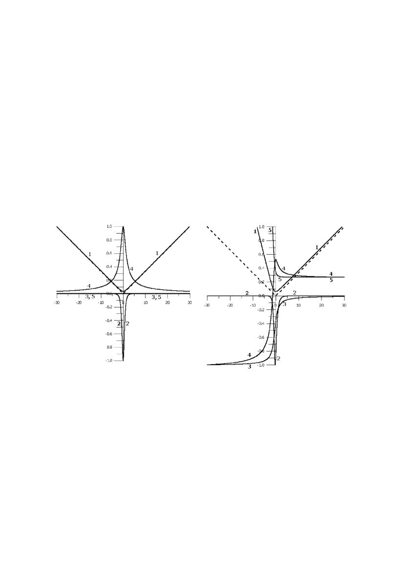
Figure 7: Analytic solution for a bridge with $w_{\parallel}=-w_{\perp}=+1$ at $l_{max}=30r_{0}$: (1) $r(l)/l_{max}$, (2) $\varepsilon(l)/|\varepsilon_{max}|$, (3) $\varphi(l)/|\varphi_{max}|$, (4) $b(l)/|b_{max}|\to r_{g}/|b_{max}|$, and (5) $a(l)\cdot const\to r_{g}/|b_{max}|$. The lines $|l|/l_{max}$ are shown dashed. The left-hand panel represents the symmetric solution for $m=0$ and the right-hand panel the asymmetric solution for $m=0.2|\eta|$.

Particular attention should be paid here to the signs $\pm$. The equation for the trajectory $\varphi(r)$ is obtained by integrating over the radius $r$. The sign of the integrand changes together with the changing sign in (47) when the point of minimum radius is passed. In the limiting case of infinite initial and final radii, the change of the angle $\varphi$ is

$$\Delta\varphi=2\int\limits_{r_{min}}^{\infty}\,{h\over r^{2}\sqrt{(1-b/r)((1-a/r)^{-1}-h^{2}/r^{2})}}\,dr\,.$$ (48)

This expression can be integrated in explicit form in two important limiting cases:

(1) $h\ll r_{0}$, $h\ll a$, $h\ll b$ is the case of when the impact parameter is sufficiently small that the photon can pass through the throat. In this case, $r_{min}=r_{0}$ and the $h^{2}/r^{2}$ term in the denominator of (48) can be neglected. Assuming that $a$ and $b$ are constant, we obtain

$$\Delta\varphi_{{}_{I}}={2h\over b}\left\{1-\sqrt{({b\over r_{0}}-1)({a\over r_{0}}-1)}+{b-a\over 2\sqrt{ab}}\ln\left[{(\sqrt{b(a-r_{0})}+\sqrt{a(b-r_{0})}(\sqrt{b}-\sqrt{a})\over(\sqrt{b(a-r_{0})}-\sqrt{a(b-r_{0})})(\sqrt{b}+\sqrt{a})}\right]\right\}\,.$$ (49)

This formula is analogous to that for a converging thin lens.

(2) $h\gg r_{0}$, $h\gg a$, $h\gg b$ is the case when the impact parameter is sufficiently large that the photon does not pass through the throat. In this case, $a\approx b\approx r_{g}$ is a constant and $r_{min}$ is determined by the equation $r^{2}_{min}+ar_{min}-h^{2}=0$. Neglecting terms quadratic in $a/h$ and $b/h$ and substituting the variable $z=r-b/2$ we obtain $z_{min}\approx h-(a+b)/2$,

$$\Delta\varphi_{{}_{II}}=\pi+{a+b\over h}\,.$$ (50)

This expression coincides with the usual formula for the gravitational lensing of photons when $a=b=r_{g}$.

When a photon trajectory corresponds to the first or second cases depends on the value of the impact parameter compared to the critical value defined by the equation

$$re^{-\phi}=h_{cr}=min\quad\makebox{ or }\quad 1-r_{cr}\phi^{\prime}(r_{cr})=0\,.$$ (51)

For example for a bridge with $w=-2$, one can find numerically that $h_{cr}\approx 2.621$.

Translated by Yu.Dumin

References

- 1. A.Einstein and N.Rosen Phys.Rev. 48 73 (1935).
- 2. M.Morris and K.Thorne Amer.J.Phys. 56, 395 (1988).
- 3. A.Carlini, V.P.Frolov, M.B.Mensky, I.D.Novikov and H.H.Soleng, gr-qc/9506087
- 4. A.D.Linde ”Elementary Particles Physics and Inflation Cosmology” (Nauka Moscow 1990) [in Russian].
- 5. A.A.Shatskiy, Zh.Eksp.Teor.Fiz. 116 (8), 353 (1999) [JETP 89 189 (1999)].
- 6. C.Armendariz-Picon, gr-qc/0201027.
- 7. Matt Visser ”Lorentzian Wormholes from Einstein to Hawking”, (United Book Baltimore USA 1996).
- 8. M.B.Bogdanov and A.M.Cherepashchuk Astron. Zh.79 1109 (2002) [Astron.Rep.46 996 (2002)].
- 9. L.D.Landau and E.M.Lifshits Field Theory (Nauka Moscow 1988) [in Russian ].
- 10. I.D.Novikov and V.P.Frolov ”Black-Holes Physics” (Nauka Moscow 1986) [in Russian ].
- 11. C.W.Misner, K.S.Thorne, and J.A.Wheeler ”Gravitation” (Freeman, San Francisco, 1973; Mir Moscow 1977), Vols. 1 .3.