The submillimeter C and CO lines in Henize 2-10 and NGC 253.

The purpose of this paper is to describe a method for determining a cooling template for galaxies, using nearby galaxies, and applicable to future observations of distant galaxies. We observed two starburst galaxies (NGC 253 and Henize 2-10) with the Caltech Submillimeter Observatory in the rotational lines of carbon monoxide ¹²CO(J=3-2), (J=6-5) and (J=7-6) for both, and also ¹²CO(J=4-3) and ¹³CO(J=3-2) for Henize 2-10 and in the ³P₂-³P₁ fine-structure transitions of atomic carbon [CI] at 809 GHz for NGC 253. Some of these observations have been made previously, but the present multitransition study (including data found in the literature) is the most complete to date for the two galaxies. From these observations, we have derived the properties of the warm and dense molecular gas in the galaxy nuclei. We used an LTE analysis and an LVG radiative transfer model to determine physical conditions of the interstellar medium in both sources and predicted integrated line properties of all CO transitions up to ¹²CO(15-14). We found the observations to be in good agreement with a medium characterized by $T_{k}\approx 50-100\text{ }K$, $\frac{{}^{12}CO}{{}^{13}CO}\approx 30$, $n(H_{2})\gtrsim 10^{4}\text{ }cm^{-3}$ and $N(^{12}CO)=3.5\pm 1.0\times 10^{18}\text{ }cm^{-2}$ for Henize 2-10 and characterized by $T_{k}\approx 70-150\text{ }K$, $\frac{{}^{12}CO}{{}^{13}CO}\approx 40$, $n(H_{2})\gtrsim 10^{4}\text{ }cm^{-3}$ and $N(^{12}CO)=1.5\pm 0.5\times 10^{19}\text{ }cm^{-2}$ for NGC 253. A PDR model has also been used and here the data are well fitted (within 20 %) by a model cloud with a gas density of n(H)= 8.0$\pm 1.0\times$ 10⁵ $cm^{-3}$ and an incident FUV flux of $\chi\approx$20000 for Henize 2-10. For NGC 253, we deduced n(H)= 3.0$\pm 0.5\times$ 10⁵ $cm^{-3}$ and $\chi\approx$20000 for the modelled cloud. The physical properties of warm gas and CO cooling curves of the target galaxies are compared with those measured for the nucleus of the Milky Way and the Cloverleaf QSO. The gas properties and CO cooling curve are similar for the two starburst galaxies and the Cloverleaf QSO while the Milky Way nucleus exhibits lower excitation molecular gas.

1 Introduction

Over the past decade, observations of distant galaxies have become possible in the millimeter and submillimeter bands and considerable progress is expected for the next decade. Much of the energy provided by star formation in those galaxies is down-converted to the submm and appears as dust emission and the familiar gas cooling lines. Because the information on distant galaxies is scarce, due to the lack of resolution and sensitivity, it is essential to understand nearby galaxies in order to provide templates for more distant objects. In recent studies of emission of fine-structure transitions of atomic carbon [CI], ionized atomic carbon [CII] and carbon monoxide (CO), we have begun to see how they relate to each other and to dust emission (Gerin & Phillips 1998, 2000). However, to estimate the relative contributions of the various species to the gas cooling, it is often necessary to make assumptions for the power in the various unobserved lines.

It is well known that the fine-structure lines of ionized carbon [CII] and atomic oxygen oxygen [OI] contribute most of the cooling of the neutral interstellar gas in galaxies. These lines trace the cooling of the diffuse neutral gas with a significant contribution from Photo-Dissociation Regions (PDRs). Fine-structure lines of ionized oxygen [OIII] and nitrogen [NII] trace the ionized gas, either in HII regions([OIII]) or the diffuse ionised gas ([NII]). In molecular gas, the cooling radiation is due to atomic carbon, carbon monoxide and water lines (although water (like most molecules) is not sufficiently widespread to contribute much cooling to a galaxy as a whole). These predictions have been confirmed by the COBE-FIRAS observations of the Milky Way: apart from [CII] and [NII] and probably [OI], the most intense submillimeter lines are from C and CO (see Fixsen et al. 1999 and Sect. 4.2). The relative contributions of the different lines of C and CO vary along the Galactic plane. Also C contributes less in proportion to the total cooling towards the Galactic Center than towards the rest of the disk (Bennett et al 1994 and Fixsen et al. 1999).

The detection of CO lines of distant galaxies remains an extremely difficult task and will continue so until ALMA is ready. However, detecting their submillimeter continuum emission is now feasible, with the advent of sensitive bolometer arrays. Due to the negative K-correction effect, the dust emission of distant galaxies piles up at submillimeter wavelengths irrespective of redshift. Additional information is needed to be able to estimate a photometric redshift, or to classify the galaxies. For instance, Yun & Carilli (2002) have proposed to use the cm radio continuum emission for obtaining photometric redshifts. From the model developed by Lagache, Dole & Puget (2003) to explain the evolution of number counts in the submillimeter and far infrared (FIR), it appears that two main galaxy populations contribute to these number counts: a relatively local population of “cold” galaxies, similar to our own galaxy, in which the continuum emission is dominated by extended disk-type emission, and an additional, strongly evolving population of infrared (IR) luminous galaxies , similar to local starburst galaxies. From the information gathered so far on high-J CO emission in galaxies (this work; Israel & Baas 2002, 2003; Bradford et al. 2003; Ward et al. 2003 and references therein), it is likely that high-J CO lines (¹²CO(4-3) and above) will be more prominent in actively star forming galaxies compared to the less active galaxies in which only low-J CO lines and the carbon lines are expected. In this paper, from an extensive set of observations of submillimeter CO lines, we conclude that, relative to ¹²CO(1-0), starburst galaxies do exhibit stronger high-excitation CO lines (¹²CO(4-3) and above), than the Milky Way galaxy.

Determining the physical conditions of molecular clouds in external galaxies can be difficult. For single-dish observations of external galaxies, the beam size is usually larger than the angular diameter of typical molecular clouds, hence the cloud emission is beam-diluted. In addition, molecular clouds are known to be clumpy (e.g. Stutzki & Guesten 1990). The intensities of CO rotational lines are sensitive to the gas physical conditions (H₂ density n(H₂), and kinetic temperature $T_{k}$), the ¹²CO column density N(¹²CO) as well as the velocity field. In this paper, we use several methods for determining the ¹²CO column density and the physical conditions, and for predicting the intensity of all CO rotational lines up to ¹²CO(15-14). The LTE analysis is useful for constraining the kinetic temperature. Using LVG models, three parameters (n(H₂),$T_{k}$, N(¹²CO)) can be measured. PDR models include a self consistent treatment of the thermal and chemical processes and provide therefore a better theoretical understanding of the gas properties.

We recall that, assuming LTE, the brightness temperature, $T_{B}$, of CO lines as a function of the kinetic temperature $T_{k}$ can be written as:

$$T_{B}=FF\left(J_{\nu}(T_{k})-J_{\nu}(T_{bg})\right)\left(1-e^{-\tau}\right)$$ (1)

where $FF$ is the source surface filling factor in the beam, $\tau$ is the line opacity, $T_{bg}$ is the CMB temperature ($T_{bg}=2.7$ $K$) and $J_{\nu}(T_{k})$ is described in Kutner & Ulich 1981 by:

$$J_{\nu}(T_{k})=\left(\frac{h\nu}{k_{b}}\right)\times\frac{1}{exp(\frac{h\nu}{k_{b}T_{k}})-1}$$ (2)

where $k_{b}$ is the Boltzmann’s constant and $h$ is the Planck constant. We show in Fig. 1 the brightness temperature, $T_{B}$, as a function of the kinetic temperature $T_{k}$. In this example, typical figures for Galactic molecular clouds have been chosen with $FF$ = 1, $N(^{12}CO)=1\times 10^{18}\text{ }cm^{-2}$ and $\Delta v=1$ $kms^{-1}$, resulting in saturated CO lines.

For a gas temperature around $T_{k}\approx 10\text{ }K$, low-J CO lines (¹²CO(1-0), ¹²CO(2-1) and ¹²CO(3-2)) are easily detected while mid and high-J CO lines (¹²CO(5-4), ¹²CO(6-5) and above) need warmer gas to be detected ($T_{k}\gtrsim 15\text{ }K$).

Since we want to sample warm gas, we have observed, for both galaxies, the high-J CO lines: ¹²CO(4-3) (only for Henize 2-10), ¹²CO(6-5) and ¹²CO(7-6) which are more sensitive to warm, dense gas directly involved in the starburst. We also observed ¹²CO(3-2) for both galaxies and ¹³CO(3-2) for Henize 2-10, to better constrain the models (see Sect. 5.1).

Atomic carbon has also proved to be a good tracer of molecular gas (Israel & Baas 2001 and Gerin & Phillips 2000). The fine structure transition of atomic carbon ³P₂-³P₁[CI] at 809 GHz for NGC 253 has also been observed here, since the intensity ratio between this line and the ³P₁-³P₀[CI] at 492 GHz is a sensitive tracer of the total gas pressure. For NGC 253, Bradford et al. (2003) and Israel, White & Baas (1995) give the intensity of the fine structure transition of atomic carbon ³P₁-³P₀[CI] at 492 GHz. For Henize 2-10, Gerin & Phillips (2000) give the intensity of the ³P₁-³P₀[CI] at 492 GHz but we could not find a measure of ³P₂-³P₁[CI] at 809 GHz to compute the line ratio.

In the following, we present new CO and CI data for NGC 253 and for Henize 2-10 (see Sect. 3). The galaxies are described in Sec. 2, the observations in Sec. 3. The results and data analysis providing ISM properties are discussed in Sec. 4 and in Sec. 5, respectively, with conclusions in section 6.

Figure 1: Brightness temperature $T_{B}$ (equations  1 and  2 in Sect. 1) vs. the kinetic temperature, $T_{k}$, assuming a unity filling factor ($FF=1$). The first curve on the left is ¹²CO(1-0) (full line) followed by ¹²CO(2-1) (triangles), ¹²CO(3-2) (squares), ¹²CO(4-3) (full line)… up to ¹²CO(15-14). For this plot, we used N(CO)= $1\times 10^{18}$ $cm^{-2}$ and $\Delta v=1$ $kms^{-1}$ resulting in $\tau>>1$.

2 The sample:

Henize 2-10 is a blue compact dwarf galaxy with a metallicity of 12+log($\frac{O}{H})\approx 8.93$ (Zaritsky, Kennicutt & Huchra 1994). It presents a double core structure suggesting a galaxy merger (Baas, Israel & Koornneef 1994). From optical, infrared and radio observations of Henize 2-10, the derived distance is 6 Mpc (Johansson 1987). Henize 2-10 is rich in neutral atomic hydrogen (Allen, Wright & Goss 1976) and harbors a considerable population of Wolf-Rayet stars (D’Odorico, Rosa & Wampler 1983; Kawara et al. 1987). Previous CO observations have been reported by Baas, Israel & Koornneef (1994); Kobulnicky et al. (1995 and 1999) and Meier et al. (2001). The starburst is confined in the galaxy nucleus within a radius of 5”(150 pc). This galaxy was chosen because it shows intense and narrow CO lines.
NGC 253 is a highly inclined galaxy (i=78^o, Pence 1980) of type Sc. With M82, it is the best nearby example of a nuclear starburst (Rieke, Lebofsky & Walker 1988). Blecha (1986) observed 24 of the brightest globular clusters and estimated a distance of 2.4 to 3.4 Mpc, while Davidge & Pritchet (1990) analysed a color-magnitude diagram of stars in the halo of NGC 253 and conclude that the distance is 1.7 to 2.6 Mpc. In the following, we shall use a value of D = 2.5 Mpc as in Mauersberger et al. (1996). NGC 253 has been extensively observed at all wavelengths (Turner 1985 (map in all four 18 cm lines of OH in the nucleus); Antonucci & Ulvestad 1988 (deep VLA maps of NGC 253 which show at least 35 compact radio sources); Carlstrom et al. 1990 (the J = 1-0 transitions of HCN and HCO⁺ and the 3 mm continuum emission); Telesco & Harper 1980 (30 and 300 $\mu$m emission); Strickland et al. 2004 (X-ray observations)). NGC 253 presents a very active and young starburst. It is among the first galaxies to have been detected in submillimeter lines and continuum. The NGC 253 nucleus has been mapped previously in various lines of CO and C (Bradford et al. 2003; Israel & Baas 2002; Sorai et al. 2000; Harrison, Henkel & Russell 1999; Israel, White & Baas 1995; Wall et al. 1991; Harris et al. 1991). The most intense emission is associated with the starburst nucleus with additional weak and extended emission from the disk (Sorai et al 2000). Both galaxies harbor superstar clusters in their nuclei (Keto et al. 1999) similar to the superstar clusters found in interacting galaxies (Mirabel et al. 1998). Basic properties for both galaxies are summarized in Table 1.

Table 1: Basic properties of Henize 2-10 and NGC 253.

$$\begin{array}[]{p{0.5\linewidth}l}\hline\cr\vskip 3.0pt plus 1.0pt minus 1.0pt\cr HENIZE 2-10&\\ \vskip 3.0pt plus 1.0pt minus 1.0pt\cr\hline\cr\vskip 3.0pt plus 1.0pt minus 1.0pt\cr RA(1950)&08:34:07.2\\ DEC(1950)&-14:26:06.0\\ Distance&6Mpc^{1}\\ Velocity (LSR)&+850\text{ }kms^{-1}\\ Optical size&30^{\prime\prime}\times 40^{\prime\prime}\\ Position Angle&130^{o}\\ Inclination&44^{o}\\ Metallicity&12+log(\frac{O}{H})\approx 8.93^{2}\\ L${}_{FIR}$&1.7\times 10^{9}\text{ }L_{\odot}\text{ }^{3}\\ Absolute Luminosity L${}_{B}$&1.2\times 10^{9}\text{ }L_{\odot}\text{ }^{4}\\ \vskip 3.0pt plus 1.0pt minus 1.0pt\cr\hline\cr\hline\cr\vskip 3.0pt plus 1.0pt minus 1.0pt\cr NGC 253&\\ \vskip 3.0pt plus 1.0pt minus 1.0pt\cr\hline\cr\vskip 3.0pt plus 1.0pt minus 1.0pt\cr RA(1950)&00:45:05.7\\ DEC(1950)&-25:33:38.0\\ Distance&2.5Mpc^{5}\\ Velocity (LSR)&+240\text{ }kms^{-1}\\ Optical size&27.5^{\prime}\times 6.8^{\prime}\\ Position Angle&51^{o}\\ Inclination&78.5^{o}\\ Metallicity&12+log(\frac{O}{H})=8.99\pm 0.31^{2}\\ L${}_{FIR}$&1.0\times 10^{10}\text{ }L_{\odot}\text{ }^{3}\\ Absolute Luminosity L${}_{B}$&2.7\times 10^{10}\text{ }L_{\odot}\text{ }^{6}\\ \vskip 3.0pt plus 1.0pt minus 1.0pt\cr\hline\cr\end{array}$$

¹: Johansson 1987
²: Zaritsky et al. 1994
³: Computed from formula in Imanishi & Dudley (2000) and from Sanders & Mirabel (1996)
⁴: Baas, Israel & Koornneef 1994
⁵: As in Mauersberger et al. 1996 (see text)
⁶: Pence 1980

3 Observations

The observations were made during various sessions at the Caltech Submillimeter Observatory (CSO) in Hawaii (USA) with the Superconducting Tunnel Junction receivers operated in double-side band mode. The atmospheric conditions varied from good ($\tau_{225}\lesssim 0.1$) to excellent ($\tau_{225}\approx$ 0.06). We used a chopping secondary mirror with a throw of 1 to 3 arcmin, depending on the size of the source, and with a frequency around 1 Hz. Henize 2-10 is point-like for all lines. The NGC 253 nucleus has a size of 50” (see Fig. 3) which is smaller than the chopping throw. For this galaxy, we used a 3’ chopping throw in ¹²CO(3-2). There is no sign of contamination by emission in the off beams. We restricted the chopping throw to 1’ for ¹²CO(6-5) and ¹²CO(7-6) as the emission is very compact in these lines. Spectra were measured with two acousto-optic spectrometers (effective bandwidth of 1000 MHz and 500 MHz). The first one has a spectral resolution about 1.5 MHz and the second one about 2 MHz. The IF frequency of the CSO receivers is 1.5 GHz. The main beam efficiencies ($\eta$) of the CSO were 69.8%, 74.6%, 51.5%, 28% and 28% at 230, 345, 460, 691 and 806 GHz respectively, as measured on planets. We used the ratio $\frac{1}{\eta}$ to convert T${}^{*}_{A}$ into T_mb. The beam size at 230, 345, 460, 691 and 806 GHz is 30.5”, 21.9”, 14.5”, 10.6” and 8.95” respectively .

The pointing was checked using planets (Jupiter, Mars and Saturn) and evolved stars (IRC 10216 and R-Hya). The pointing accuracy is around 5”. The overall calibration accuracy is 20%. Data have been reduced using the CLASS data analysis package. The spectra have been smoothed to a velocity resolution of 10 kms^-1 and linear baselines have been removed.

For NGC 253, we obtained spectra towards the central position for both ¹²CO(7-6) line and the atomic carbon CI(³P₂-³P₁) line simultaneously. We observed 70 positions in the ¹²CO(3-2) line and 20 positions for the ¹²CO(6-5) line. For Henize 2-10 we observed only the nucleus for the ¹²CO(3-2), ¹²CO(4-3), ¹²CO(6-5), ¹²CO(7-6) and ¹³CO(3-2) lines. The carbon line ³P₁-³P₀ [CI] is from Gerin & Phillips (2000).

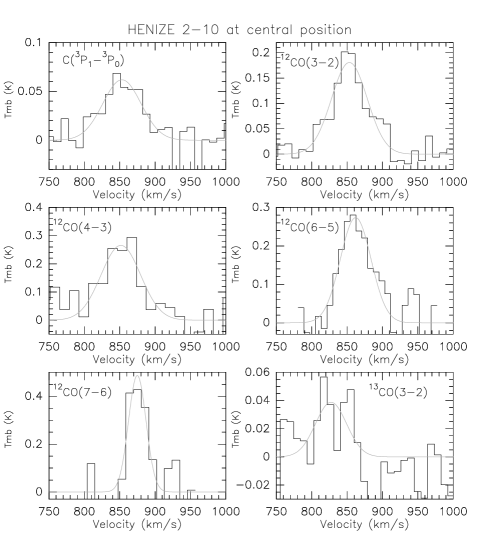
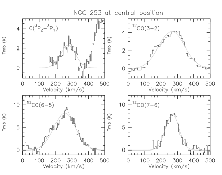
Figure 2: Spectra of Henize 2-10 (top six) and NGC 253 (bottom four) at central positions as given in Table 1. Velocities (horizontal axis) are given relative to the LSR (V_LSR) in $kms^{-1}$ and the line intensities (vertical axis) are in units of T_mb ($K$). The grey curves are Gaussian fits. For NGC 253, the line on the right hand side of CI(³P₂-³P₁) is the edge of ¹²CO(7-6) line seen in the image side band.

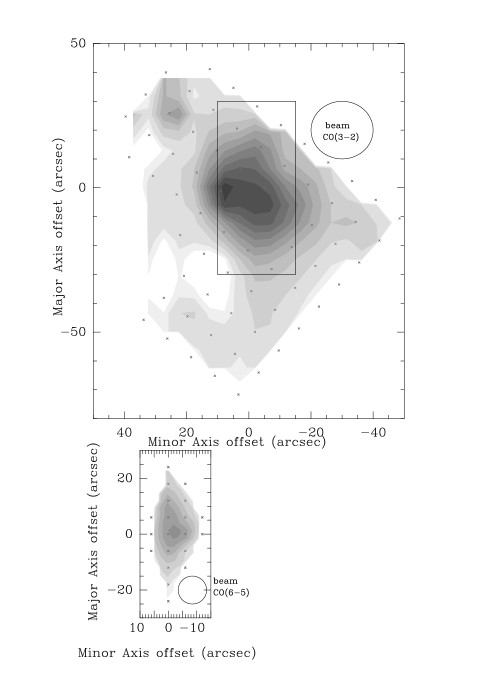
Figure 3: Map of the velocity integrated intensity of ¹²CO(3-2) (Top) and ¹²CO(6-5) (Bottom) towards NGC 253 nucleus. The CO emission is integrated over the full velocity range - 100 to 700 $kms^{-1}$ and 60 to 400 $kms^{-1}$, respectively. For both maps, missing grid positions are interpolated and the crosses show the observed positions. The first and the second contours of the ¹²CO(3-2) map are of 41.6 $Kkms^{-1}$ and 81.6 $Kkms^{-1}$ respectively; others contours range from $\int{T_{mb}dv}$ = 81.6 to 816 $Kkms^{-1}$ in steps of 81.6 $Kkms^{-1}$. For the ¹²CO(6-5) map, contours are of 43 $Kkms^{-1}$, 141 $Kkms^{-1}$, 282 $Kkms^{-1}$, 564 $Kkms^{-1}$, 846 $Kkms^{-1}$, 1128 $Kkms^{-1}$ and 1410 $Kkms^{-1}$. The peak value of the ¹²CO(3-2) map is $\int{T_{mb}dv}\approx 816$ $Kkms^{-1}$. The peak value of the ¹²CO(6-5) map is $\int{T_{mb}dv}\approx 1400$ $Kkms^{-1}$. The maps are rotated by 51⁰ to match the major axis position angle of the CO emission in NGC 253. The ¹²CO(3-2) map has been shifted by -5” in minor axis offset (see text in Sect. 3 and in Sect. 4.1). The black box in the upper figure represents the size of the lower figure.

Table 2: Results for Henize 2-10.

HENIZE 2-10
Transition	Freq	Beam Size	$\int(T_{mb}dv)$	Intensity	Flux	Referencesa
	(GHz)	(”)	(Kkms-1)	(Wm-2sr-1)	(Wm-2)
CI(3P1-3P0)	492.162	14.55	4.2$\pm$0.8	5.1$\times 10^{-10}$	3.0$\times 10^{-18}$	4 & 5b
		21.90	2.5$\pm$0.5	3.0$\times 10^{-10}$	3.8$\times 10^{-18}$	4 & 5b
12CO(1-0)	115.271	40.00	10.0$\pm$0.8	1.6$\times 10^{-11}$	6.7$\times 10^{-19}$	1
		21.90	27.3$\pm$2.2	4.3$\times 10^{-11}$	5.5$\times 10^{-19}$	1
		55.00	4.9$\pm$0.2	7.6$\times 10^{-12}$	6.1$\times 10^{-19}$	2
		21.90	23.9$\pm$1.0	3.7$\times 10^{-11}$	4.8$\times 10^{-19}$	2*
12CO(2-1)	230.538	21.00	17.3$\pm$1.4	2.2$\times 10^{-10}$	2.5$\times 10^{-18}$	1*
		27.00	6.8$\pm$0.8	8.5$\times 10^{-11}$	1.7$\times 10^{-18}$	2
		21.90	9.4$\pm$1.1	1.2$\times 10^{-10}$	1.5$\times 10^{-18}$	2
12CO(3-2)	345.796	21.90	11.5$\pm$2.3	4.9$\times 10^{-10}$	6.2$\times 10^{-18}$	5*
		21.00	23.2$\pm$2.1	9.8$\times 10^{-10}$	1.2$\times 10^{-17}$	1
		22.00	16.6$\pm$0.6	7.0$\times 10^{-10}$	9.0$\times 10^{-18}$	3
12CO(4-3)	461.041	14.55	18.6$\pm$4.2	1.9$\times 10^{-9}$	1.1$\times 10^{-17}$	5
		21.90	10.9$\pm$2.4	1.1$\times 10^{-9}$	1.4$\times 10^{-17}$	5*
12CO(6-5)	691.473	10.60	15.7$\pm$3.1	5.3$\times 10^{-9}$	1.6$\times 10^{-17}$	5
		21.90	6.8$\pm$1.3	2.3$\times 10^{-9}$	2.9$\times 10^{-17}$	5*
12CO(7-6)	806.652	8.95	15.2$\pm$3.0	8.2$\times 10^{-9}$	1.7$\times 10^{-17}$	5
		21.90	5.8$\pm$1.2	3.1$\times 10^{-9}$	4.0$\times 10^{-17}$	5*
13CO(1-0)	110.201	40.00	$<$ 0.5	$<$ 6.8$\times 10^{-13}$	$<$ 2.9$\times 10^{-20}$	1
		21.90	$<$ 1.4	$<$ 1.8$\times 10^{-12}$	$<$ 2.4$\times 10^{-20}$	1
		57.00	0.3$\pm$0.1	3.9$\times 10^{-13}$	3.4$\times 10^{-20}$	2
		21.90	1.6$\pm$0.5	2.2$\times 10^{-12}$	2.8$\times 10^{-20}$	2*
13CO(2-1)	220.399	21.00	0.9$\pm$0.2	9.9$\times 10^{-12}$	1.2$\times 10^{-19}$	1*
13CO(3-2)	330.588	14.00	2.3$\pm$0.6	8.5$\times 10^{-11}$	4.4$\times 10^{-19}$	1
		21.90	1.3$\pm$0.3	4.8$\times 10^{-11}$	6.1$\times 10^{-19}$	1*
		21.90	1.8$\pm$0.5	6.7$\times 10^{-11}$	8.5$\times 10^{-19}$	5

^a References: 1: Baas, Israel & Koornneef 1994; 2: Kobulnicky et al. 1995; 3: Meier et al. 2001; 4: Gerin & Phillips 2000; 5: this work; *: used for models. ^b We analysed again spectra from Gerin & Phillips 2000.

Table 3: Results for the nucleus of NGC 253.

NGC253
Transition	Freq	Beam Size	$\int(T_{mb}dv)$	Intensity	Flux	Referencesa
	(GHz)	(”)	(Kkms-1)	(Wm-2sr-1)	(Wm-2)
CI(3P1-3P0)	492.162	10.20	575.0$\pm$115.0b	7.0$\times 10^{-8}$	1.9$\times 10^{-16}$	5
		21.90	204.0$\pm$41.0	2.5$\times 10^{-8}$	3.2$\times 10^{-16}$	5
		43.00	98.0$\pm$19.6b	1.2$\times 10^{-8}$	5.9$\times 10^{-16}$	5
		22.00	290.0$\pm$45	3.5$\times 10^{-8}$	4.6$\times 10^{-16}$	10*
		23.00	320.0$\pm$64.0b	3.9$\times 10^{-8}$	5.5$\times 10^{-16}$	4
CI(3P2-3P1)	809.902	8.95	188.5$\pm$37.7	1.0$\times 10^{-7}$	2.2$\times 10^{-16}$	11
		21.9	58.1$\pm$11.6	3.2$\times 10^{-8}$	4.0$\times 10^{-16}$	11*
12CO(1-0)	115.271	43.00	343.0$\pm$68.6b	5.4$\times 10^{-10}$	2.6$\times 10^{-17}$	2
		23.00	920.0$\pm$82.8	1.4$\times 10^{-9}$	2.0$\times 10^{-17}$	6*
12CO(2-1)	230.538	23.00	1062.0$\pm$116.8	1.3$\times 10^{-8}$	1.9$\times 10^{-16}$	7*
		21.00	926.0$\pm$185.2b	1.2$\times 10^{-8}$	1.4$\times 10^{-16}$	2
12CO(3-2)	345.796	21.90	815.6$\pm$163.1	3.5$\times 10^{-8}$	4.4$\times 10^{-16}$	11*
		23.00	998.0$\pm$139.7	4.2$\times 10^{-8}$	5.9$\times 10^{-16}$	7
		23.00	1194.0$\pm$238.8b	5.0$\times 10^{-8}$	7.1$\times 10^{-16}$	2
		14.00	1200.0$\pm$240.0b	5.1$\times 10^{-8}$	2.6$\times 10^{-16}$	5
		21.90	618.9$\pm$123.8	2.6$\times 10^{-8}$	3.3$\times 10^{-16}$	5
		22.00	680.0$\pm$60.0	2.9$\times 10^{-8}$	3.7$\times 10^{-16}$	8
12CO(4-3)	461.041	15.00	507.0$\pm$101.4b	5.1$\times 10^{-8}$	3.0$\times 10^{-16}$	3
		21.90	285.3$\pm$57.1	2.9$\times 10^{-8}$	3.7$\times 10^{-16}$	3
		22.00	1019.0$\pm$120	1.0$\times 10^{-7}$	1.3$\times 10^{-15}$	9*
		10.40	2160.0$\pm$432.0b	2.1$\times 10^{-7}$	6.2$\times 10^{-16}$	5
		21.90	786.2$\pm$157.2	7.9$\times 10^{-7}$	1.0$\times 10^{-15}$	5
12CO(6-5)	691.473	10.60	1394$\pm$278.8	4.7$\times 10^{-7}$	1.4$\times 10^{-15}$	11
		21.90	518.3$\pm$104.3	1.8$\times 10^{-7}$	2.2$\times 10^{-15}$	11*
		8/30	861$\pm$258.3	2.9$\times 10^{-7}$	5.0$\times 10^{-15}$	1
12CO(7-6)	806.652	8.95	810.2$\pm$162.0	4.3$\times 10^{-7}$	9.3$\times 10^{-16}$	11
		21.90	249.9$\pm$50.3	1.3$\times 10^{-7}$	1.7$\times 10^{-15}$	11*
		11.5/60	1370$\pm$411	7.3$\times 10^{-7}$	2.6$\times 10^{-15}$	10
13CO(1-0)	110.201	23.00	80$\pm$8.0	1.1$\times 10^{-10}$	1.5$\times 10^{-18}$	7*
13CO(2-1)	220.399	23.00	82$\pm$9.8	9.0$\times 10^{-10}$	1.3$\times 10^{-17}$	7*
		21.00	104$\pm$20.8b	1.1$\times 10^{-9}$	1.3$\times 10^{-17}$	2
13CO(3-2)	330.588	23.00	90$\pm$12.6	3.3$\times 10^{-9}$	4.7$\times 10^{-17}$	7*
		23.00	210$\pm$42.0b	7.8$\times 10^{-9}$	1.1$\times 10^{-16}$	2

^a References: 1: Harris et al. 1991; 2: Wall et al. 1991; 3: Guesten et al. 1993; 4: Harrison et al. 1995; 5: Israel, White & Baas 1995; 6: Mauersberger et al. 1996; 7: Harrison, Henkel & Russell 1999; 8: Dumke et al. 2001; 9: Israel & Baas 2002; 10: Bradford et al. 2003; 11: this work; *: used for models.
^b The error is not given in the referenced paper. It has been estimated to be 20%.

4 Data analysis

4.1 Spectra and maps:

Henize 2-10 and NGC 253 spectra at central positions are shown in Fig. 2; Fig. 3 shows ¹²CO(3-2) and ¹²CO(6-5) maps of NGC 253. We detected ¹²CO(3-2), ¹²CO(6-5) and ¹²CO(7-6) in both galaxies. For these positions, line intensities (A in $Kkms^{-1}$ and I in $Wm^{-2}sr^{-1}$) and line fluxes (F in $Wm^{-2}$) resulting from Gaussian fits are listed in Table 2 and in Table 3, together with the beam size of the observations. Because of likely pointing offsets ($\approx$ 5” from pointing scans on planets and evolved stars) between different observing runs, we believe that differences in the peak positions of ¹²CO(3-2) and ¹²CO(6-5) in NGC 253 are partly due to pointing errors. But we can not exclude that a difference in peak positions remains after the pointing correction (see Fig. 3). Three peaks appear on the high resolution ¹²CO(1-0) maps obtained with the Nobeyama Interferometer (NRO), one near the center and two on each side at around 3 ” south-west and 8 ” north-east respectively (Paglione et al, 2004). The offset peak in the ¹²CO(3-2) map may be associated with the north-east secondary peak. Table 2 and Table 3 also report relevant data found in the literature. For some spectra, a Gaussian may not represent the true line profile but given the weakness of the signal, fitting anything more complicated is not warranted.
To be able to compare intensities of the different CO lines, we have also computed the line intensities (A and I) and fluxes (F) for a common beam size of 21.9”, which is the size of the ¹²CO(3-2) beam at the CSO. They are listed in Table 2 and in Table 3 and identified with an asterisk in column 7 (named References). To do so, we have used the following assumptions:

• Henize 2-10: we modelled the source with an axisymmetric Gaussian distribution, with a full width half maximum (FWHM) of 13”, as found by Meier et al. 2001.

• NGC 253: we made use of the ¹²CO(6-5) map to determine the source size at 690 GHz and model the emission at higher frequencies. We modelled the nucleus as an elliptical source with Gaussian intensity profiles. The ¹²CO(6-5) map can be well fitted with such a model, with half maximum width of 23” along the major axis and 11” along the minor axis, which is very similar to the size of the CS(J=2-1) emission in the nucleus (Peng et al. 1996). The source appears to be resolved along the major axis but unresolved along the minor axis. We used the same source model for ¹²CO(7-6) and CI(³P₂-³P₁), as it fits our restricted data set.

• I is derived using the formula:

  $$\text{I}=\frac{2\times k_{b}\times\nu^{3}}{c^{3}}\times\text{A}$$ (3)

  $$\text{I}(Wm^{-2}sr^{-1})=1.02\times 10^{-18}\times\left(\frac{\nu}{GHz}\right)^{3}\times\left(\frac{A}{Kkms^{-1}}\right)$$ (4)

  where c is the speed of light, $\nu$ is the line frequency in $GHz$ and A is the line area in $Kkms^{-1}$.
  To derive the flux, F in $Wm^{-2}$, we multiply I in $Wm^{-2}sr^{-1}$ by the beam solid angle $\Omega(B)$ in sr defined as:

  $$\Omega(B)=1.133\times\text{B}^{2}\times\frac{1}{206265^{2}}\text{ }sr$$ (5)

  where B is the half power beam width (HPBW) in arcsec. The estimated error for our data in Table 2 and in Table 3 is about 20%.
  

4.2 C and CO cooling:

Our observations are designed to provide essential information on the cooling and consequently on the thermal balance of the interstellar medium in Henize 2-10 and NGC 253. We shall also deduce which CO line(s) contribute the most to the total observed CO cooling and estimate the total observed cooling of C and CO by summing intensities in $Wm^{-2}sr^{-1}$ of all transitions listed in Table 2 and in Table 3 with asterisks (both literature data and our dataset). We have computed the observed C and CO cooling in the galaxy nuclei for a beam size of 21.9”, this corresponds to linear scales of 640 pc and 270 pc for Henize 2-10 and NGC 253 respectively.
For Henize 2-10 and NGC 253 we measured a total observed CO cooling rate of $7.2\times 10^{-9}\text{ }Wm^{-2}sr^{-1}$ and $4.6\times 10^{-7}\text{ }Wm^{-2}sr^{-1}$ respectively. For NGC 253 the lines contributing the most to the observed CO cooling are ¹²CO(6-5) (39.2% of the total intensity) followed by ¹²CO(7-6) (28.3%). For Henize 2-10, it is ¹²CO(7-6) (43.1%) followed by ¹²CO(6-5) (31.9%).
The observed total cooling rates of neutral carbon C for Henize 2-10 and NGC 253 are respectively $3.0\times 10^{-10}\text{ }Wm^{-2}sr^{-1}$ (CI(³P₁-³P₀) transition only) and $6.7\times 10^{-8}\text{ }Wm^{-2}sr^{-1}$ (for NGC 253, CI(³P₂-³P₁) represents 52.2% of the total).
These results show that ¹²CO(6-5) and ¹²CO(7-6) are contributing the most to the total observed CO cooling, with very similar percentages for both galaxies. It is natural to wonder whether ¹²CO(5-4) and ¹²CO(8-7) are strong also. This will be investigated in Sec. 5.2 and Sec. 5.3.
In starburst nuclei, CO cooling is larger than C cooling by a factor of $>10$, which explains why it is easier to detect CO than C in distant galaxies. Similar results have been obtained on J1148+5251 (z=6.42) and on PSS2322+1944 (z=4.12) (Bertoldi et al (2003), Walter et al. (2003) and Cox et al. (2002)). Barvainis et al (1997) detected CI(³P₁-³P₀) (3.6 $\pm$ 0.4 $Jykms^{-1}$) in the Cloverleaf quasar at redshift z=2.5. In the same quasar, Wei$\beta$ et al (2003) detected CI(³P₂-³P₁) (5.2 $\pm$ 0.3 $Jykms^{-1}$) and ¹²CO(3-2) (13.2 $\pm$ 0.2 $Jykms^{-1}$). In distant objects, C cooling also seems to be weaker than CO cooling.

5 CO models:

In this section, we use the measured CO line ratios and intensities (I and A) to determine the physical conditions of molecular gas, namely the kinetic temperature, the gas density, the CO column density and the FUV flux: $\chi$. In the first section, we start with an LTE analysis. In Sect. 5.2, we use an LVG radiative transfer model and in Sect. 5.3, we discuss the use of a PDR model. In the last section, we discuss the similarities and differences between the two galaxies, the nucleus of the Milky Way and the distant QSO “the Cloverleaf”. The latter has been chosen as being representative of distant, actively star forming galaxies.

5.1 LTE analysis:

In the local thermodynamical equilibrium (LTE) approximation, we assume that CO is thermalized, hence the relative populations of its energy levels are functions of the kinetic temperature (assumed uniform) only. We discuss two limiting cases, applied to ¹²CO and ¹³CO:

• the lines are optically thick (optical depth: $\tau\gg 1$); the line intensity ratio (eg $\frac{{}^{12}CO(3-2)}{{}^{12}CO(2-1)}$) can be written:

  $$R^{thick}_{32/21}=\frac{FF\times T^{12}CO(3-2)}{FF\times T^{12}CO(2-1)}=\frac{J_{\nu 32}(T_{k})-J_{\nu 32}(T_{bg})}{J_{\nu 21}(T_{k})-J_{\nu 21}(T_{bg})}$$ (6)

  with $J_{\nu}(T_{k})$ defined as in Eq 2 in Sec. 1. In LTE, $R^{thick}_{32/21}\approx 1$ and $R^{thick}_{76/65}\approx 1$ for $T_{k}>30\text{ }K$, while $R^{thick}_{65/32}\approx 1$ and $R^{thick}_{76/32}\approx 1$ for $T_{k}>100\text{ }K$. Plots of the line intensity ratios ($R^{thick}$) as a function of the kinetic temperature $T_{k}$ for the optically thick case in the LTE approximation are given in Fig. 4. From this figure, we conclude that the line ratios combining high-J (¹²CO(6-5) or ¹²CO(7-6)) with low-J (¹²CO(3-2)) lines are the most useful for constraining the kinetic temperature.
  

  

  Figure 4: Integrated intensity lines ratios, $R^{thick}$, (defined as in Eq. 6), vs kinetic temperature in K. We assume LTE, and optically thick lines (optical depth, $\tau\gg 1$).

• One line is optically thick and the other is optically thin; this is likely when comparing line intensities for different isotopologues of CO in the same J transition (eg ${}^{12}CO(3-2)$/${}^{13}CO(3-2)$). Assuming equal excitation temperatures for both species, optically thin ¹³CO lines and optically thick ¹²CO lines, we get:

  $$R_{12/13}=\frac{FF\times T^{12}CO}{FF\times T^{13}CO}\approx\frac{A(^{12}CO)}{A(^{13}CO)}\approx\frac{1}{\tau(^{13}CO)}$$ (7)

  $$\hskip 39.83368pt\approx\frac{X_{galaxy}}{\tau(^{12}CO)}$$ (8)

  where $X_{galaxy}$ is the ¹²CO/¹³CO abundance ratio. Previous work, using LVG models, found, for Henize 2-10, $X\simeq 30$ (Baas, Israel & Koornneef 1994) and for NGC 253, $X\simeq 40$ (Henkel & Mauersberger 1993; Henkel et al. 1993 and Israel & Baas 2002). From the literature data, summarized in Table 2, and in Table 3, we deduced $\tau(^{12}$CO$(1-0))\simeq 2.0$ and $\tau(^{12}$CO$(2-1))\simeq 1.6$ for Henize 2-10. For NGC 253, we obtained $\tau(^{12}$CO$(1-0))\simeq 3.5$ and $\tau(^{12}$CO$(2-1))\simeq 3.1$ ($\tau$ increase for larger $X_{galaxy}$: assuming $X_{NGC253}\simeq 50$ as in Bradford et al. (2003) $\tau(^{12}$CO$(1-0))\simeq 4.3$ and $\tau(^{12}$CO$(2-1))\simeq 3.9$.

  Unfortunately, the opacity of the ¹²CO(3-2) line for both galaxies is not accurately determined due to systematic differences between data sets (Baas, Israel & Koornneef 1994; Harrison, Henkel & Russell 1999 and this work). For Henize 2-10, $\tau(^{12}$CO$(3-2))$ ranges between 1.7 and 3.4, and for NGC 253, it ranges between 3.0 and 5.8 for the abundance ratio given above ($X_{NGC253}=40$). We note that the largest error is for the ¹³CO integrated intensity which is the most difficult line to observe: for NGC 253, A(¹³CO(3-2)) varies between $90\text{ }Kkms^{-1}$ (Harrison, Henkel & Russell 1999) and $210\text{ }Kkms^{-1}$ (Wall et al. 1991) while A(¹²CO(3-2)) varies between $619\text{ }Kkms^{-1}$ (Israel, White & Baas 1995) and $1194\text{ }Kkms^{-1}$ (Wall et al. 1991) (at the same resolution).

Because the observed ratio is $R^{thick}_{65/32}\approx 0.6$ for both Henize 2-10 and NGC 253 (see Table 4), we conclude, from the LTE analysis, that the ¹²CO(3-2) line opacities are moderate ($1<\tau<10$) and the gas is warm ($T_{k}>30\text{ }K$).
To go further and constrain the gas density, we now use LVG models.

5.2 LVG model:

The detection of the high-excitation CO lines directly indicates the presence of large amounts of warm and dense gas in these galaxies. The CO excitation is modelled in terms of standard, one-component, spherical LVG radiative transfer model with uniform kinetic temperature and density (Goldreich & Kwan 1974; De Jong, Dalgarno & Chu 1975). Though the assumption of uniform physical conditions is crude, these models represent a useful step in predicting intensities of the submillimeter CO lines, since, in any case, we lack information concerning the gas distribution in the galaxy, particularly its small scale structure.

There are four main variables in LVG models: the CO column density divided by the line width: N(¹²CO)/$\Delta v$, the molecular hydrogen density: n(H₂), the kinetic temperature: $T_{k}$ and the $\frac{{}^{12}\text{CO}}{{}^{13}\text{CO}}$ abundance ratio: $X_{galaxy}$. The linewidth, $\Delta v$, is constrained by the fit of the ¹²CO(3-2) spectra (FWHM). We have used $\Delta v=60\text{ }kms^{-1}$ for Henize 2-10 and $\Delta v=190\text{ }kms^{-1}$ for NGC 253 (see Fig. 2). The $\frac{{}^{12}\text{CO}}{{}^{13}\text{CO}}$ abundance ratio varies between 30 and 40 for Henize 2-10 ($X_{Henize2-10}$) and between 30 and 50 for NGC 253 ($X_{NGC253}$).
To make quantitative estimates of the physical parameters of the molecular gas in nuclei, we have compiled information about line emission for all CO rotational transitions observed so far and scaled them to a common beam size of 21.9”(see Table 2 and Table 3 and Sec. 4.1).

Model solutions for the physical parameters, for both sources, are presented in Table 5. Because acceptable fits can be obtained over a large domain of parameter space, we have chosen to present two models which bracket the range of possible solutions for the kinetic temperature. The first one has a “low kinetic temperature” ($T_{K}<80\text{ }K$), shown with crosses in Figs. 5 and  6) and the second one has a “high $T_{K}$” ($T_{K}>100\text{ }K$), shown with triangles in Figs. 5 and  6) (see Table  4). The gas density is not well constrained but must be at least $10^{4}\text{ }cm^{-3}$. The best fit ¹²CO/¹³CO value is 30 for Henize 2-10 and 40 for NGC 253, both compatible with previous analyses. We varied N(¹²CO) from $1.0\times 10^{16}\text{ }cm^{-2}$ to $1.0\times 10^{20}\text{ }cm^{-2}$ for Henize 2-10 and $3.5\times 10^{17}\text{ }cm^{-2}$ to $3.5\times 10^{19}\text{ }cm^{-2}$ for NGC 253. CO column densities are mainly constrained by the ¹³CO data (see Table 2 and Table 3). Acceptable fits are found : N(¹²CO)=$3.5\pm 1\times 10^{18}\text{ }cm^{-2}$ for Henize 2-10 and for N(¹²CO)=$1.5\pm 0.5\times 10^{19}\text{ }cm^{-2}$ for NGC 253. We determined the “best” fit using a least square fit method for the line area ratios listed in Table 4. As we wanted to derive the properties of warm gas, we have given more weight to line ratios which include high-J CO lines, e.g. $\frac{{}^{12}CO(3-2)}{{}^{12}CO(6-5)}$, $\frac{{}^{12}CO(3-2)}{{}^{12}CO(7-6)}$ and $\frac{{}^{12}CO(6-5)}{{}^{12}CO(7-6)}$ (see Sect. 5.1).

Predicted line integrated areas, A in $Kkms^{-1}$ and line intensities I in $Wm^{-2}sr^{-1}$ for all CO transitions to J=15-14, are also shown in Figs. 5 and  6. The predicted line area A is obtained by multiplying the antenna temperature, given by models, by the line width $\Delta v$ and by the surface filling factor, FF. For each observed CO line, we estimated the surface filling factor (FF) of molecular clouds in the beam using the ratio $T_{mb}(observations)/T_{mb}(model)$. We made an average, weighted by the S/N, for the FF pertaining to each observed transition. For Henize 2-10 and NGC 253, we obtained filling factors of $FF=8.8\pm 3\times 10^{-3}$ and $FF=8.7\pm 3\times 10^{-2}$ respectively. The line intensities, I, are derived from the model A values through Eq. 3 and Eq. 4. We give in Table 4, line intensity ratios of CO transitions derived from observations and from models.

The low-J CO transitions (¹²CO(1-0) and ¹²CO(2-1)) are not well fit by the adopted LVG models, because we have chosen to constrain the models with high-J transitions of CO as we are interested in the warm gas properties. In order to study the properties of the low excitation molecular gas, we could have introduced another gas component in the models as in Harrison, Henkel & Russel (1999) or Bradford et al. (2003) for NGC 253. Here, the LVG models predict too low an intensity for the ¹²CO(1-0) and ¹²CO(2-1) lines in this source, supporting the need for a low excitation gas component. For NGC 253, we obtained a similar kinetic temperature $T_{K}$ as in Bradford et al. 2003, but a lower density $n(H_{2})$ and a higher CO column density N(¹²CO). For NGC 253, Paglione et al. (2004) found good fits with LVG models with N(¹²CO)/$\Delta v$ between $4.0\times 10^{16}\text{ }cm^{-2}km^{-1}s$ and $1.3\times 10^{18}\text{ }cm^{-2}km^{-1}s$, in good agreement with our value (N(¹²CO)/$\Delta v=8.0\times 10^{16}\text{ }cm^{-2}km^{-1}s$). Recent measurements of rotational lines of H₂ (Rigopoulou et al. 2002) suggest that warm gas with $T_{K}\simeq 150\text{ }K$ is present in NGC 253 which is compatible with our models.

The LVG models have been used for predicting the CO line intensities for ¹²CO(1-0) up to ¹²CO(15-14). We have derived the total CO cooling from these predictions. For Henize 2-10, we obtain with the “low $T_{K}$” model ($T_{K}=50\text{ }K$), $1.3\times 10^{-8}\text{ }Wm^{-2}sr^{-1}$, and with the “high $T_{K}$” model ($T_{K}=100\text{ }K$), $2.0\times 10^{-8}\text{ }Wm^{-2}sr^{-1}$. With the “low $T_{K}$” model, the lines which contribute the most to the total CO cooling are ¹²CO(6-5) (23.4%), followed by ¹²CO(5-4) (19.7%) and ¹²CO(7-6) (19.5%). With the “high $T_{K}$” model, the lines which contribute the most to the total CO cooling are ¹²CO(7-6) (19.1%) followed by ¹²CO(6-5) (18.2%) and ¹²CO(8-7) (15.4%).

For NGC 253, with the “low $T_{K}$” model ($T_{K}=70\text{ }K$) we deduced a total CO cooling of $1.0\times 10^{-6}\text{ }Wm^{-2}sr^{-1}$ and the most important line is ¹²CO(7-6) (21.1%) followed by ¹²CO(6-5) (20.4%), ¹²CO(8-7) (15.7%) and ¹²CO(5-4) (15.2%). With the “high $T_{K}$” model ($T_{K}=150\text{ }K$), we obtained a total predicted CO cooling of $1.5\times 10^{-6}\text{ }Wm^{-2}sr^{-1}$, with the most intense lines being ¹²CO(8-7) and ¹²CO(7-6) (16.4% for each) followed by ¹²CO(6-5) (13.6%) and ¹²CO(9-8) (13.4%).

¹²CO(6-5) and ¹²CO(7-6) therefore appear to contribute significantly to the CO cooling. Also, CO lines with $J_{upper}\geqslant 10$ are predicted to be weak and will not have significant antenna temperatures (see Figs. 5 and  6, plots on the left side). In addition to ¹²CO(6-5) and ¹²CO(7-6), data for ¹²CO(8-7) and ¹²CO(9-8) would be most useful in discriminating between models, and for a more accurate determination of the CO cooling. ¹³CO(6-5) data would also be extremely useful for constraining the models and for measuring the opacity of ¹²CO(6-5) line.

Table 4: Observed and predicted (“low $T_{K}$” and “high $T_{K}$” LVG models) line area ratios for Henize 2-10 and NGC 253.

A	NGC 253	HENIZE 2-10
($Kkms^{-1}$)	observations	observations
$\frac{{}^{12}CO(3-2)}{{}^{12}CO(6-5)}$	1.6$\pm$0.6∗	1.7$\pm$0.7∗
$\frac{{}^{12}CO(3-2)}{{}^{12}CO(7-6)}$	3.3$\pm$1.3∗	2.0$\pm$0.8∗
$\frac{{}^{12}CO(6-5)}{{}^{12}CO(7-6)}$	2.1$\pm$0.8∗	1.2$\pm$0.5∗
$\frac{{}^{12}CO(1-0)}{{}^{13}CO(1-0)}$	11.5$\pm$2.2∗	14.9$\pm$5.8∗
$\frac{{}^{12}CO(2-1)}{{}^{13}CO(2-1)}$	13.0$\pm$3.0∗	19.2$\pm$5.8∗
$\frac{{}^{12}CO(3-2)}{{}^{13}CO(3-2)}$	9.1$\pm$3.1∗	8.9$\pm$3.8∗
	“low $T_{K}$” model	“low $T_{K}$” model
	$T_{K}=70\text{ }K$	$T_{K}=50\text{ }K$
$\frac{{}^{12}CO(3-2)}{{}^{12}CO(6-5)}$	1.6	2.0
$\frac{{}^{12}CO(3-2)}{{}^{12}CO(7-6)}$	2.5	3.8
$\frac{{}^{12}CO(6-5)}{{}^{12}CO(7-6)}$	1.5	1.9
$\frac{{}^{12}CO(1-0)}{{}^{13}CO(1-0)}$	25.5	19.1
$\frac{{}^{12}CO(2-1)}{{}^{13}CO(2-1)}$	13.4	9.9
$\frac{{}^{12}CO(3-2)}{{}^{13}CO(3-2)}$	10.1	8.1
	“high $T_{K}$” model	“high $T_{K}$” model
	$T_{K}=150\text{ }K$	$T_{K}=100\text{ }K$
$\frac{{}^{12}CO(3-2)}{{}^{12}CO(6-5)}$	1.4	1.6
$\frac{{}^{12}CO(3-2)}{{}^{12}CO(7-6)}$	1.8	2.5
$\frac{{}^{12}CO(6-5)}{{}^{12}CO(7-6)}$	1.3	1.5
$\frac{{}^{12}CO(1-0)}{{}^{13}CO(1-0)}$	15.1	23.9
$\frac{{}^{12}CO(2-1)}{{}^{13}CO(2-1)}$	20.7	14.8
$\frac{{}^{12}CO(3-2)}{{}^{13}CO(3-2)}$	14.8	9.9

^∗ : ratio derived from observations marked with asterisks in Table 2 and in Table 3.

Table 5: Parameters of the “best” LVG models.

	Henize 2-10	NGC 253
n(H2) (cm-3)	$\gtrsim$1 $\times$ 104	$\gtrsim$1 $\times$ 104
N(12CO) (cm-2)	3.5$\pm$1 $\times$ 1018	1.5$\pm$0.5 $\times$ 1019
$\frac{{}^{12}C}{{}^{13}C}$	30	40
$\Delta v^{*}$ (kms-1)	60	187
$T_{K}$ (K)	50-100	70-150
FF	8.8$\pm$3 $\times$ 10-3	8.7$\pm$3 $\times$ 10-2

^∗ deduced from Gaussian fits to the ${}^{12}CO(3-2)$ line profiles.

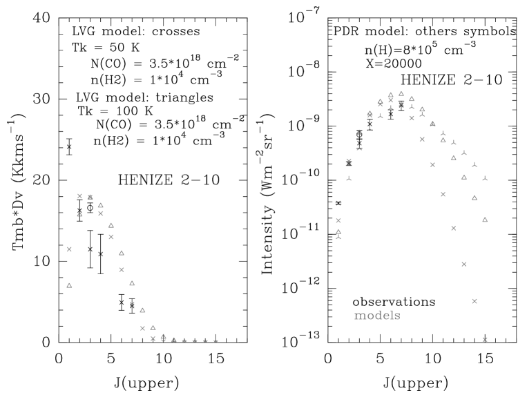
Figure 5: LVG and PDR model calculations compared with observations for Henize 2-10. On the left side, we plot integrated intensities in $Kkms^{-1}$ vs J_upper. On the right side, we plot I in $Wm^{-2}sr^{-1}$ vs J_upper. In both figures, grey crosses represent the “low temperature” LVG model while grey triangles represent the “high temperature” LVG model. The starred grey triangles represent results of the PDR model (see Sect. 5.3). Observations (with error bars) taken from literature and from our data set are shown in black. We have reported two observations for ${}^{12}CO(3-2)$ in Henize 2-10: the black cross is from our data and the black circle is from Meier et al. 1991. The last one seems to be agree better with the model predictions. As Henize 2-10 is a point source, a small pointing error can explain this difference.

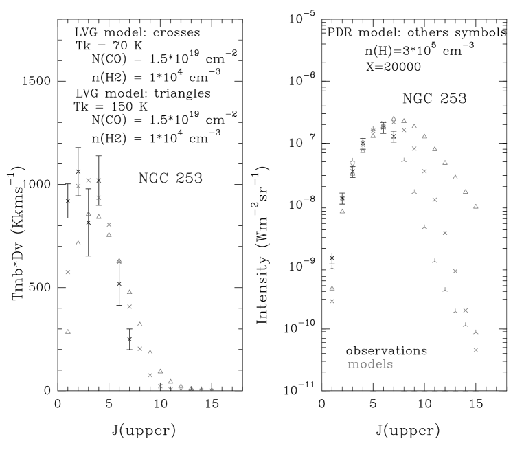
Figure 6: LVG and PDR models calculations compared with observations for NGC 253. The observations are shown in black with error bars while model predictions are shown in grey. See caption of Fig. 5.

5.3 PDR model:

To progress further in the analysis of the physical conditions in the starburst nuclei, we made use of PDR models. Such models have been used here to understand the properties of the interstellar medium, since they take account of all the relevant physical and chemical processes for thermal balance. The PDR models accurately reproduce the steep kinetic temperature gradient near cloud edges, when illuminated by intense FUV radiation. Such models have been developed during the past two decades, for a variety of astrophysical sources, from giant molecular clouds illuminated by the interstellar radiation field to the conditions experienced by circumstellar disks, very close to hot massive stars (Tielens & Hollenbach 1985; Van Dishoeck & Black 1986, 1988; Wolfire, Hollenbach & Tielens 1990; Hollenbach, Takahashi & Tielens 1991; Abgrall et al. 1992; Le Bourlot at al. 1993; Köster et al. 1994; Sternberg & Dalgarno 1995; Draine & Bertoldi 1996, Stoerzer et al. 1996, Lhuman et al. 1997; Pak et al. 1998; Hollenbach & Tielens 1999 and Kaufman et al. 1999).

We adopted here the PDR model developed by Le Bourlot et al. (1993) for Galactic sources (see also Le Petit, Roueff & Le Bourlot 2002) . The source is modelled as a plane-parallel slab, illuminated on both sides by FUV radiation to better reproduce the starburst environment as massive stars and giant molecular clouds are spatially correlated. Model parameters include the gas density, assumed uniform, the intensity of the illuminating FUV radiation, the gas phase elemental abundances, the grain properties, the gas to dust ratio, etc. Because the metallicities of both NGC 253 and Henize 2-10 (see Table 1) are close to solar, we used a model with Milky Way abundances ($12+log(\frac{O}{H})=$8.90 $\pm$ 0.04 Boselli, Lequeux & Gavazzi 2002). We have adopted standard grain properties and gas to dust ratio appropriate for Galactic interstellar clouds. We have sampled a wide range of the parameter space, varying the gas density, n(H) and the incident FUV flux, $\chi\times G_{0}$, where $G_{0}$ is the local average interstellar radiation field (ISRF) determined by Draine (1978) ($G_{0}=2.7\times 10^{-3}\text{ }ergcm^{-2}s^{-1}$). The ¹²C/¹³C ratios ($X_{Henize2-10}$ and $X_{NGC253}$) are the same as for the “best” LVG models (see Table 5). Models are constrained by the ratio of integrated intensities in $ergcm^{-2}s^{-1}sr^{-1}$ listed in Table 2 and in Table 3 ($E$($ergcm^{-2}s^{-1}sr^{-1}$) = $I(Wm^{-2}sr^{-1})\times 10^{3}$).
Parameter pairs (n(H); $\chi$) which fit our dataset, are listed in Table 6. $\chi$ seems to be constrained by the ¹²CO(J+1$\rightarrow$J)/¹³CO(J+1$\rightarrow$J)(e.g. ¹²CO(3-2)/¹³CO(3-2)) ratios while n(H) is more sensitive to the line ratios involving two ¹²CO lines: ¹²CO(J+1$\rightarrow$J)/¹²CO(J’+1$\rightarrow$J’)(e.g. ¹²CO(3-2)/¹²CO(6-5)) ratio. The difference between observations and model outputs is estimated to be of the order of 20%. Emissivity ratios obtained from the observations and from the models are listed in Table 7.

Model predictions for the CO line emissivities are shown in Fig. 5 and Fig. 6 for Henize 2-10 and NGC 253 respectively. The model predictions have been scaled to match the observed line intensities. As stated above, PDR models have been developed for local interstellar clouds. The velocity dispersion of the modelled cloud is a parameter in those models, which is used for computing the photo-dissociation rates of H₂ and CO, and the line emissivities. This parameter is set to 1 $kms^{-1}$, a typical figure for local molecular clouds (see Wolfire, Tielens & Hollenbach 1990). Using a PDR model for fitting the galaxy observations is complicated by the fact that, in a galaxy, many PDRs contribute to the signal detected in each beam, resulting in a broad line (tens to hundred of kms^-1), compared to a single PDR line (1 kms^-1). To correct for this effect, the model line emissivities have been multiplied by the line width ratio, $\frac{\Delta v(galaxy)}{\Delta v(PDR)}$, where $\Delta v(galaxy)\approx 190\text{ }kms^{-1}$ and $60\text{ }kms^{-1}$ for NGC 253 and Henize 2-10 respectively, and $\Delta v(PDR)=1\text{ }kms^{-1}$. Once this correction is performed, PDR model results are compared with observed data in the same way as the LVG models (see paragraph 5 in Sect. 5.2), and the surface filling factor of the emission in the beam, PDR_FF, is computed. The PDR_FF is 9.4$\times 10^{-2}$ for NGC 253 and 1.5 $\times 10^{-3}$ for Henize 2-10. For NGC 253, the surface filling factors derived from the PDR and the LVG models are very similar. For Henize 2-10, the filling factor is significantly smaller for the PDR model than for the LVG model. In Henize 2-10, LVG models, as with PDR models, do not reproduce observations very well due to the lack of high-J CO lines (i.e., ¹²CO(8-7) and up) which would constrain the location of the maximum of the CO cooling curve. However, compared to LVG models, PDR models tend to fit the series of CO lines better, particularly for NGC 253. So, we prefer the PDR values of the FF to those from the LVG.

We have computed the total CO cooling from PDR models summing the contribution from all CO lines from ¹²CO(1-0) up to ¹²CO(15-14). In the observations, we miss ¹²CO(5-4) and all CO lines from ¹²CO(8-7) and up. For Henize 2-10, we obtained $1.5\times 10^{-8}\text{ }Wm^{-2}sr^{-1}$ (similar to the CO cooling from the “low $T_{K}$” LVG model ($T_{K}=50\text{ }K$)). The lines which contribute the most to the total CO cooling are ¹²CO(7-6) (17.4%) followed by ¹²CO(8-7) (15.7%) and ¹²CO(6-5) (15.0%) (with the “low $T_{K}$” LVG model, the lines which contribute the most are also CO lines with $J_{upper}\geqslant 5$). For NGC 253, we deduced a total CO cooling of $7.2\times 10^{-7}\text{ }Wm^{-2}sr^{-1}$, (close to, but lower than the CO cooling from the “low $T_{K}$” LVG model ($T_{K}=70\text{ }K$)). The most important line is ¹²CO(6-5) (24.9%) followed by ¹²CO(5-4) (23.2%) and ¹²CO(7-6) (17.0%).
For NGC 253, the cooling derived from the PDR model is $\approx 40$% higher than the observed CO cooling, while for Henize 2-10, the cooling from PDR models is a factor of 2 larger than the measured value. This can be explained by the fact that, for Henize 2-10, PDR models do not fit observations as well as for NGC 253. Actually, ¹²CO(8-7) or ¹²CO(9-8), and ¹³CO(6-5) or ¹³CO(7-6), would be very useful in order to determine the position of the peak of the CO cooling curve, and the opacity of the ¹²CO(6-5) or ¹²CO(7-6) lines. Finally, the strong dependence of the PDR model fit with the density n(H), as can be seen by comparing Fig. 5 and Fig. 6, might also explain the difference between the two galaxies. We discuss this point in the next section.

Table 6: Parameters of the “best” PDR models.

	Henize 2-10	NGC 253
n(H) (cm-3)	8.0$\pm 1\times$ 105	3.0$\pm 0.5\times$ 105
$\chi$ (on each side)	20000	20000a
$v^{b}$ (kms-1)	60	187
FF	1.5$\pm 0.5\times 10^{-3}$	9.7$\pm 4\times 10^{-2}$

^a Carral et al. (1994) found for NGC 253 a FUV flux of 2$\times 10^{4}G_{o}$ in units of Habing (1968) corresponding to 1.2$\times 10^{4}G_{o}$ in units of Draine (1978); compatible with our value.
^b deduced from Gaussian fits to line profiles.

Table 7: Observed and modeled line emissivity ratios for Henize 2-10 and NGC 253 using PDR models.

E	NGC 253	HENIZE 2-10
($ergcm^{-2}s^{-1}sr^{-1}$)	observations	observations
$\frac{{}^{12}CO(3-2)}{{}^{12}CO(6-5)}$	0.19$\pm 0.076^{*}$	0.22$\pm 0.083^{*}$
$\frac{{}^{12}CO(3-2)}{{}^{12}CO(7-6)}$	0.27$\pm 0.11^{*}$	0.16$\pm 0.064^{*}$
$\frac{{}^{12}CO(6-5)}{{}^{12}CO(7-6)}$	1.38$\pm 0.56^{*}$	0.74$\pm 0.29^{*}$
$\frac{{}^{12}CO(1-0)}{{}^{13}CO(1-0)}$	12.73$\pm 2.5$∗	16.82$\pm 6.2^{*}$
$\frac{{}^{12}CO(2-1)}{{}^{13}CO(2-1)}$	14.44$\pm 3.4$∗	22.22$\pm 6.1^{*}$
$\frac{{}^{12}CO(3-2)}{{}^{13}CO(3-2)}$	10.61$\pm 3.6$∗	10.21$\pm 4.7^{*}$
	model	model
$\frac{{}^{12}CO(3-2)}{{}^{12}CO(6-5)}$	0.26	0.18
$\frac{{}^{12}CO(3-2)}{{}^{12}CO(7-6)}$	0.34	0.15
$\frac{{}^{12}CO(6-5)}{{}^{12}CO(7-6)}$	1.32	0.86
$\frac{{}^{12}CO(1-0)}{{}^{13}CO(1-0)}$	15.42	15.07
$\frac{{}^{12}CO(2-1)}{{}^{13}CO(2-1)}$	9.72	8.02
$\frac{{}^{12}CO(3-2)}{{}^{13}CO(3-2)}$	7.92	6.27

^∗ : ratio derived from observations marked with asterisks in Table 2 and Table 3.

5.4 Discussion

From the models described above, we conclude that the molecular gas in the starburst regions of Henize 2-10 and NGC 253 experience similar physical conditions: both the line ratios and derived properties are similar. Nevertheless, we can see in Fig. 5 and in Fig. 6, a density difference between the two galaxies. In fact, it is difficult to fit a PDR model for Henize 2-10 since we do not have a CO detection for J higher than J=7-6. The reason is the large intensity of the ¹²CO(7-6) line relative to ¹²CO(6-5). When the turn over in the CO cooling curve is not well constrained, fitting one PDR model is not easy and the solution can be understood as a “lower limit”.
Moreover lower transitions of carbon monoxide like ¹²CO(1-0) and ¹²CO(2-1) were not really essential here since models were dedicated to the study of warm gas. So, the detection of high-J transitions was crucial for describing the starburst nuclei.
Another point is the influence of the FWHM line width. It is obvious for NGC 253 that the FWHM of the ¹²CO(3-2) line ($\approx 190kms^{-1}$) is larger than that of the ¹²CO(7-6) line ($\approx 95kms^{-1}$), the main reason being the better spatial resolution of the ¹²CO(7-6) data. Because NGC 253 has a steep velocity gradient along its major axis, the convolution to lower spatial resolution, using the adopted source model, is expected to produce broader lines profiles. We tried to take into account this phenomenon in our study by using LVG models with ratios in line integrated area in $Kkms^{-1}$ instead of using ratios in main beam temperature in $K$. We also studied LVG models with a smaller $\Delta v$ but this implies a lower N(CO) since the meaningful variable in LVG models is the CO column density divided by the line width: N(¹²CO)/$\Delta v$. So different parameter pairs (N(¹²CO), $\Delta v$) may reproduce the observations equally well.
PDR models predict the emissivity of the CI(³P₁-³P₀) and the CI(³P₂-³P₁), fine structure transitions of atomic carbon at 492 $GHz$ and 809 $GHz$ respectively (see Table 8). For Henize 2-10, the predicted CI(³P₁-³P₀) line emissivity is brighter than the observed value by a factor of 2. For NGC 253, the predicted transitions are brighter than those observed by a factor of 3 for CI(³P₁-³P₀) and a factor of 12 for the CI(³P₂-³P₁). We concluded that PDR models fitted to the CO line emission do not reproduce the atomic carbon data very well. Perhaps, to better constrain models with observed atomic carbon transitions, we should reduce the density. The fine-structure lines of atomic carbon seem to share the same behaviour as the low-J CO transitions. This tendancy is found in Galactic clouds also.
We compared observations of CO and [CI] in the center of the Milky Way (Fixsen et al. 1999), and in the Cloverleaf QSO (Barvainis et al. 1994, Tsuboi et al. 1999 and Wei$\beta$ et al. 2003) with our observations. These two objects are well known and we can compare them with NGC 253 and Henize 2-10, to determine the differences or the similarities in the physical properties of their warm gas. We chose to plot CO lines fluxes (F in $Wm^{-2}$) versus J_upper, instead of CO lines intensities (I in $Wm^{-2}sr^{-1}$) versus J_upper as in Fig. 5 and in Fig. 6, because the Milky Way data found in Fixsen et al. (1999) were only available in these units. The Cloverleaf QSO data (in $Jykms^{-1}$ in Barvainis et al. 1994, Tsuboi et al. 1999 and Wei$\beta$ et al. 2003) have been converted to the same units using the Jy per K factors and the main beam efficiencies of telescopes (see references above). Line fluxes (F in $Wm^{-2}$) are listed in Table 9 and the flux ratios in Table 10.
CO line fluxes (F in $Wm^{-2}$) for the Cloverleaf QSO, the nucleus of the Milky Way, NGC 253 and Henize 2-10 are shown in Fig. 7. To compare the CO cooling curves more easily, the line fluxes have been scaled. The scaling factors are listed in the figure caption. In Fig. 7, PDR model predictions have been used for the CO lines which are lacking observations: ¹²CO(5-4) and ¹²CO(8-7) for NGC 253 and for Henize 2-10 (see Table 9). Note that the PDR model used for Henize 2-10 PDR does not reproduce observations as well as the PDR model used for NGC 253 (see Fig. 5 and Fig. 6).
We compare the CO cooling curve for the center of the Milky Way, the Cloverleaf QSO, Henize 2-10 and NGC 253. The turnover positions for Henize 2-10, NGC 253 and the Cloverleaf QSO are close to each other, near ¹²CO(6-5) or above, while the turnover of the CO cooling curve of the nucleus of the Milky Way is near ¹²CO(4-3). We may ask if this observed difference between the Milky Way and the three other sources is consistent with a difference in linear resolution, or if it is due to differences in inherent physical conditions between the four environments. The linear resolution for NGC 253 corresponding to the adopted beam size of 21.9” is 265 pc. For Henize 2-10, with a distance of 6 Mpc and the same beam size, we obtained a linear resolution of 637 pc. For the Cloverleaf QSO, we computed the angular distance from $H_{0}$ and $q_{0}$ in Wei$\beta$ et al. (2003), we obtained $D_{A}=1056.4$ Mpc and a linear resolution of 13 kpc. For the nucleus of the Milky Way, the 7⁰ COBE-FIRAS beam gives a linear resolution of 1035 pc in the Galactic Center (distance of 8.5 kpc). We conclude that despite the wide range of linear resolutions, the turnover of the CO cooling curve is found at roughly the same J value, above ¹²CO(6-5) for Henize 2-10, NGC 253 and the Cloverleaf QSO. However, at the same linear scale as Henize 2-10, the gas in the Milky Way nucleus shows less excitation. Thus, it seems likely that differences in the shapes of the CO cooling curves are due to differences in the ISM properties in the target galaxies. The fact that the Cloverleaf QSO, NGC 253 and Henize 2-10 have the same ratios is related to the similarity of the physical properties of warm gas for these three sources, which translates into similar CO line ratios (see Table 10).

Table 8: Results of PDR models for [CI] in Henize 2-10 and NGC 253. We reported also observations from Table 2 and 3. The PDR model predictions have been multiplied by the line width ratio, $\frac{\Delta v(galaxy)}{\Delta v(PDR)}$, and by the surface filling factor, PDR_FF, (see Table 6).

E	NGC 253	HENIZE 2-10
($ergcm^{-2}s^{-1}sr^{-1}$)	observations	observations
CI(3P1-3P0)	3.5$\times$ 10-5	3.0$\times$ 10-7
CI(3P2-3P1)	3.2$\times$ 10-5	not observed
	PDR model	PDR model
CI(3P1-3P0)	1.1$\times$ 10-4	5.1$\times$ 10-7
CI(3P2-3P1)	3.9$\times$ 10-4	1.9$\times$ 10-6

Table 9: Observations of the Milky Way nucleus (from Fixsen et al. 1999), NGC 253 (from this paper), Henize 2-10 (from this paper) and the Cloverleaf QSO (from Barvainis et al. 1994, Tsuboi et al. 1999 and Wei$\beta$ et al. 2003).

F	Milky Way	NGC 253	HENIZE 2-10	Cloverleaf
($Wm^{-2}$)
CI(3P1-3P0)	1.9$\times$ 10-10	4.6$\times$ 10-16	3.8$\times$ 10-18	1.7$\times$ 10-23
CI(3P2-3P1)	1.9$\times$ 10-10	4.0$\times$ 10-16	not observed	3.9$\times$ 10-23
12CO(1-0)	2.7$\times$ 10-11	2.0$\times$ 10-17	4.8$\times$ 10-19	$\leq$1.5$\times$ 10-24
12CO(2-1)	1.1$\times$ 10-10	1.9$\times$ 10-16	2.5$\times$ 10-18
12CO(3-2)	2.0$\times$ 10-10	4.4$\times$ 10-16	9.0$\times$ 10-18a	4.3$\times$ 10-23
12CO(4-3)	3.0$\times$ 10-10	1.3$\times$ 10-15	1.4$\times$ 10-17	9.11$\times$ 10-23
12CO(5-4)	2.8$\times$ 10-10	2.2$\times$ 10-15b	3.3$\times$ 10-17b	1.3$\times$ 10-22
12CO(6-5)	1.9$\times$ 10-10	2.2$\times$ 10-15	2.9$\times$ 10-17
12CO(7-6)	1.7$\times$ 10-10	1.7$\times$ 10-15	4.0$\times$ 10-17	3.6$\times$ 10-22
12CO(8-7)	1.8$\times$ 10-10	6.7$\times$ 10-16b	4.9$\times$ 10-17b

^a: We chose to use ¹²CO(3-2) observations from Meier et al. (2001) because they seem to agree with LVG and PDR models (see Fig. 5) better than our observations.
^b:These values are computed from PDR models.

Table 10: Flux ratios for the center of the Milky Way, NGC 253, Henize 2-10 and the Cloverleaf QSO.

F	Milky Way	NGC 253	HENIZE 2-10	Cloverleaf
($Wm^{-2}$)
$\frac{CI(^{3}P_{1}-^{3}P_{0})}{CI(^{3}P_{2}-^{3}P_{1})}$	1.00	1.15	not observed	0.42
$\frac{{}^{12}CO(3-2)}{{}^{12}CO(1-0)}$	7.37	22	18.75	$\geq$ 28.6
$\frac{{}^{12}CO(3-2)}{{}^{12}CO(2-1)}$	1.84	2.32	3.6	-
$\frac{{}^{12}CO(3-2)}{{}^{12}CO(4-3)}$	0.67	0.34	0.64	0.47
$\frac{{}^{12}CO(3-2)}{{}^{12}CO(5-4)}$	0.72	0.21∗	0.27∗	0.33
$\frac{{}^{12}CO(3-2)}{{}^{12}CO(6-5)}$	1.03	0.20	0.31	-
$\frac{{}^{12}CO(3-2)}{{}^{12}CO(7-6)}$	1.18	0.26	0.23	0.12
$\frac{{}^{12}CO(3-2)}{{}^{12}CO(8-7)}$	1.09	0.66∗	0.18∗	-

^∗:These values are computed from PDR models.

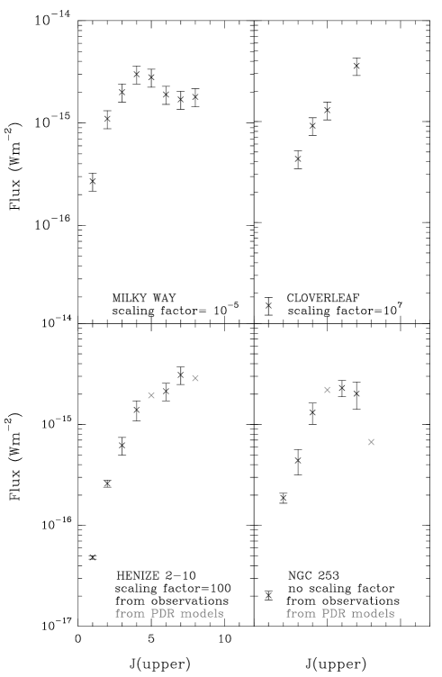
Figure 7: Flux ($Wm^{-2}$) vs. $J_{upper}$ for the nucleus of the Milky Way (top left), NGC 253 (top right), Henize 2-10 (bottom left) and the Cloverleaf QSO (bottom right). PDR models have been used to obtained fluxes (plotted in grey) of ¹²CO(5-4) and ¹²CO(8-7) in Henize 2-10 and in NGC 253. Observations are shown in black. To facilitate the comparison, we applied scaling factors of $1\times 10^{7}$ for the Cloverleaf QSO data, $1\times 10^{-5}$ for the nucleus of the Milky Way, and 100 for Henize 2-10. Data for NGC 253 are shown with no scaling factor. For the Cloverleaf QSO, the ¹²CO(1-0) line flux is an upper limit (see Tsuboi et al. 1999).

6 Conclusions:

We observed Henize 2-10 in the rotational lines of carbon monoxide ¹²CO(J=3-2), (J=4-3), (J=6-5) and (J=7-6) and NGC 253 in the ³P₂-³P₁ fine structure transitions of atomic carbon [CI] at 809 GHz and in the rotational lines of carbon monoxide ¹²CO(3-2), (J=6-5) and (J=7-6). We show that C cooling is less than CO cooling for both galaxy nuclei by a factor $>$ 10. Among observed lines, those which contribute most to the CO cooling are ¹²CO(6-5) and ¹²CO(7-6).
Such high-J transitions are needed to constrain the physical conditions in starburst nuclei. We used both LVG and PDR models for each galaxy: the molecular gas in the Henize 2-10 nucleus is well described with a LVG model defined by $\Delta V$ = 60 kms^-1, $T_{k}\approx 50-100\text{ }K$, $\frac{{}^{12}CO}{{}^{13}CO}\approx 30$, $n(H_{2})\gtrsim 10^{4}\text{ }cm^{-3}$ and $N(^{12}CO)=3.5\pm 1\times 10^{18}\text{ }cm^{-2}$. For the NGC 253 nucleus, we derived the following parameters: $\Delta V$ = 190 kms^-1, $T_{k}\approx 70-150\text{ }K$, $\frac{{}^{12}CO}{{}^{13}CO}\approx 40$, $n(H_{2})\gtrsim 10^{4}\text{ }cm^{-3}$ and $N(^{12}CO)=1.5\pm 0.5\times 10^{19}\text{ }cm^{-2}$. PDR models provide equally good fits to the data. PDR models were used to give us more information about the physical parameters in these media. We succeeded in reproducing the observations with an accuracy of about 20% using a PDR model defined for Henize 2-10 by n(H)=$8.0\pm 1\times 10^{5}$ $cm^{-3}$ and $\chi=20000$ (we modelled the source as a plane-parallel slab, illuminated on both sides by FUV radiation). For NGC 253, we derived the following model: n(H)=$3.0\pm 0.5\times 10^{5}$ $cm^{-3}$ and $\chi=20000$.
Thanks to those models, we predict that, for distant galaxies, to obtain properties of cold and warm gas, the most interesting CO lines to be observed are ¹²CO(1-0), (2-1), (3-2), (4-3), (5-4), (6-5), (7-6) and ¹²CO(8-7). ¹²CO(9-8) and higher-J CO lines will be weaker and more difficult to detect in distant galaxies. The reasons are twofold. First the most intense lines are ¹²CO(6-5) and ¹²CO(7-6), second, though ¹²CO(9-8) can have a significant contribution to the cooling, its antenna temperature is significantly lower than for other CO lines (eg ¹²CO(4-3) or ¹²CO(6-5)). Also, the typical $T_{K}$ and n($H_{2}$) values only allow significant excitation over a large fraction of the galaxy for J${}_{up}\leqslant$10 transitions. For higher-J transitions the values of $T_{K}$ and n($H_{2}$) high enough to excite J${}_{up}\geqslant$10 will be confined to a volume too small to produce a detectable signal.
Data on the ¹²CO(8-7) and on the ¹³CO(6-5) lines would be extremely useful in further studies; ¹²CO(8-7) will help to localize the maximum of the CO cooling curve, while ¹³CO(6-5) will help constrain the warm gas column density. Even now, it is still difficult to detect these lines from the ground; with APEX receivers which may cover atmospheric windows up to a frequency of 1.4 THz , these lines could become available. ALMA will give access to better spatial resolution, for resolving individual molecular clouds : And with HIFI and PACS on board the Herschel satellite, lines with frequencies up to 5 THz will become accessible.
We compared properties of warm gas derived from our models with the properties of the nucleus of the Milky Way and of the Cloverleaf QSO. We concluded that the ISM in NGC 253, Henize 2-10 and in the Cloverleaf QSO are similar, leading to similar CO excitation, while the nucleus of the Milky Way exhibits lower excitation CO lines.

- (1) Abgrall, H., Le Bourlot, J., Pineau Des Forets, G., et al., 1992, A&A, 253, 525
- (2) Allen, D. A., Wright, A. E., & Goss, W. M., 1976, MNRAS, 177, 91
- (3) Antonucci, R. R. J. & Ulvestad, J. S., 1988, ApJ, 330, L97
- (4) Arimoto, N., Sofue, Y., & Tsujimoto, T., 1996, PASJ, 48, 275
- (5) Baas, F., Israel, F. P., & Koornneef, J., 1994, A&A, 284, 403
- (6) Barvainis, R., Maloney, P., Antonucci, R., & Alloin, D., 1997, ApJ, 484, 695
- (7) Bennett, C. L., Fixsen, D. J., Hinshaw, G., et al., 1994, ApJ, 434, 587
- (8) Bertoldi, F., Cox, P., Neri, R., et al., 2003, A&A, 409, L47
- (9) Blecha, A., 1986, A&A, 154, 321
- (10) Boselli, A., Lequeux, J., & Gavazzi, G., 2002, A&A, 384, 33
- (11) Bradford, C. M., Nikola, T., Stacey, G. J., et al., 2003, ApJ, 586, 891
- (12) Carlstrom, J. E., Jackson, J. M., Ho, P. T. P., & Turner, J. L., 1990, NASA, Ames Research Center, The Interstellar Medium in External Galaxies: Summaries of Contributed Papers p 337-339 (SEE N91-14100 05-90), 337
- (13) Carral, P., Hollenbach, D. J., Lord, S. D., et al., 1994, ApJ, 423, 223
- (14) Cox, P., Omont, A., Djorgovski, S. G., et al., 2002, A&A, 387, 406
- (15) Davidge, T. J. & Pritchet, C. J., 1990, AJ, 100, 102
- (16) De Jong, T., Dalgarno, A., & Chu, S.-I., 1975, ApJ, 199, 69
- (17) D’Odorico, S., Rosa, M., & Wampler, E. J., 1983, A&AS, 53, 97
- (18) Draine, B. T. & Bertoldi, F., 1996, ApJ, 468, 269
- (19) Draine, B. T., 1978, ApJS, 36, 595
- (20) Fixsen, D. J., Bennett, C. L., & Mather, J. C., 1999, ApJ, 526, 207
- (21) Frerking, M. A., Langer, W. D., & Wilson, R. W., 1982, ApJ, 262, 590
- (22) Gerin, M. & Phillips, T. G., 1998, ApJ, 509, L17
- (23) Gerin, M. & Phillips, T. G., 2000, ApJ, 537, 644
- (24) Goldreich, P. & Kwan, J., 1974, ApJ, 189, 441
- (25) Goldsmith, P. F., 2001, ApJ, 557, 736
- (26) Goldsmith, P. F. & Langer, W. D., 1978, ApJ, 222, 881
- (27) Guesten, R., Serabyn, E., Kasemann, C., et al., 1993, ApJ, 402, 537
- (28) Habing, H. J., 1968, Bull. Astron. Inst. Netherlands, 19, 421
- (29) Harris, A. I., Stutzki, J., Graf, U. U., et al., 1991, ApJ, 382, L75
- (30) Harrison, A., Puxley, P., Russell, A., & Brand, P., 1995, MNRAS, 277, 413
- (31) Harrison, A., Henkel, C., & Russell, A., 1999, MNRAS, 303, 157
- (32) Henkel, C. & Mauersberger, R., 1993, A&A, 274, 730
- (33) Henkel, C., Mauersberger, R., Wiklind, T., et al., 1993, A&A, 268, L17
- (34) Hollenbach, D. J. & Tielens, A. G. G. M., 1999, Reviews of Modern Physics, 71, 173
- (35) Hollenbach, D. J., Takahashi, T., & Tielens, A. G. G. M., 1991, ApJ, 377, 192
- (36) Imanishi, M. & Dudley, C. C., 2000, ApJ, 545, 701
- (37) Israel, F. P. & Baas, F., 2001, A&A, 371, 433
- (38) Israel, F. P. & Baas, F., 2002, A&A, 383, 82
- (39) Israel, F. P. & Baas, F., 2003, A&A, 404, 495
- (40) Israel, F. P., White, G. J., & Baas, F., 1995, A&A, 302, 343
- (41) Johansson, I., 1987, A&A, 182, 179
- (42) Kaufman, M. J., Wolfire, M. G., Hollenbach, D. J., & Luhman, M. L., 1999, ApJ, 527, 795
- (43) Kawara, K., Nishida, M., Taniguchi, Y., & Jugaku, J., 1987, PASP, 99, 512
- (44) Keto, E., Hora, J. L., Fazio, G. G., Hoffmann, W., & Deutsch, L., 1999, ApJ, 518, 183
- (45) Kobulnicky, H. A., Dickey, J. M., Sargent, A. I., Hogg, D. E., & Conti, P. S., 1995, AJ, 110, 116
- (46) Kobulnicky, H. A., Kennicutt, R. C., & Pizagno, J. L., 1999, ApJ, 514, 544
- (47) Koester, B., Stoerzer, H., Stutzki, J., & Sternberg, A., 1994, A&A, 284, 545
- (48) Kutner, M. L. & Ulich, B. L., 1981, ApJ, 250, 341
- (49) Lagache, G., Dole, H., & Puget, J.-L., 2003, MNRAS, 338, 555
- (50) Le Bourlot, J., Pineau des Forets, G., Roueff, E., & Schilke, P., 1993, ApJ, 416, L87
- (51) Le Petit, F., Roueff, E., & Le Bourlot, J., 2002, A&A, 390, 369
- (52) Luhman, M. L., Jaffe, D. T., Sternberg, A., Herrmann, F., & Poglitsch, A., 1997, ApJ, 482, 298
- (53) Mauersberger, R., Henkel, C., Wielebinski, R., Wiklind, T., & Reuter, H.-P., 1996, A&A, 305, 421
- (54) Meier, D. S., Turner, J. L., Crosthwaite, L. P., & Beck, S. C., 2001, AJ, 121, 740
- (55) Mirabel, I. F., Vigroux, L., Charmandaris, V., et al., 1998, A&A, 333, L1
- (56) Paglione, T. A. D., Yam, O., Tosaki, T., & Jackson, J. M., 2004, ArXiv Astrophysics e-prints, astro-ph/0405031
- (57) Pak, S., Jaffe, D. T., van Dishoeck, E. F., Johansson, L. E. B., & Booth, R. S., 1998, ApJ, 498, 735
- (58) Pence, W. D., 1980, ApJ, 239, 54
- (59) Peng, R., Zhou, S., Whiteoak, J. B., Lo, K. Y., & Sutton, E. C., 1996, ApJ, 470, 821
- (60) Rieke, G. H., Lebofsky, M. J., & Walker, C. E., 1988, ApJ, 325, 679
- (61) Rigopoulou, D., Kunze, D., Lutz, D., Genzel, R., & Moorwood, A. F. M., 2002, A&A, 389, 374
- (62) Sanders, D. B. & Mirabel, I. F., 1996, ARA&A, 34, 749
- (63) Sorai, K., Nakai, N., Kuno, N., Nishiyama, K., & Hasegawa, T., 2000, PASJ, 52, 785
- (64) Sternberg, A. & Dalgarno, A., 1995, ApJS, 99, 565
- (65) Stoerzer, H., Stutzki, J., & Sternberg, A., 1996, A&A, 310, 592
- (66) Strickland, D. K., Heckman, T. M., Colbert, E. J. M., Hoopes, C. G., & Weaver, K. A., 2004, ApJS, 151, 193
- (67) Stutzki, J. & Guesten, R., 1990, ApJ, 356, 513
- (68) Telesco, C. M. & Harper, D. A., 1980, ApJ, 235, 392
- (69) Tielens, A. G. G. M. & Hollenbach, D., 1985, ApJ, 291, 747
- (70) Tielens, A. G. G. M. & Hollenbach, D., 1985, ApJ, 291, 722
- (71) Tsuboi, M., Miyazaki, A., Imaizumi, S., & Nakai, N., 1999, PASJ, 51, 479
- (72) Turner, B. E., 1985, ApJ, 299, 312
- (73) van Dishoeck, E. F. & Black, J. H., 1986, ApJS, 62, 109
- (74) van Dishoeck, E. F. & Black, J. H., 1988, ApJ, 334, 771
- (75) Wall, W. F., Jaffe, D. T., Bash, F. N., & Israel, F. P., 1991, ApJ, 380, 384
- (76) Walter, F., Bertoldi, F., Carilli, C., et al., 2003, Nature, 424, 406
- (77) Ward, J. S., Zmuidzinas, J., Harris, A. I., & Isaak, K. G., 2003, ApJ, 587, 171
- (78) Wei, A., Henkel, C., Downes, D., & Walter, F., 2003, A&A, 409, L41
- (79) Wilson, C. D., 1995, ApJ, 448, L97
- (80) Wolfire, M. G., Tielens, A. G. G. M., & Hollenbach, D., 1990, ApJ, 358, 116
- (81) Yun, M. S. & Carilli, C. L., 2002, ApJ, 568, 88
- (82) Zaritsky, D., Kennicutt, R. C., & Huchra, J. P., 1994, ApJ, 420, 87