“Mariage des Maillages”:
A new numerical approach for 3D relativistic core collapse simulations

Abstract

We present a new three-dimensional general relativistic hydrodynamics code which is intended for simulations of stellar core collapse to a neutron star, as well as pulsations and instabilities of rotating relativistic stars. Contrary to the common approach followed in most existing three-dimensional numerical relativity codes which are based in Cartesian coordinates, in this code both the metric and the hydrodynamics equations are formulated and solved numerically using spherical polar coordinates. A distinctive feature of this new code is the combination of two types of accurate numerical schemes specifically designed to solve each system of equations. More precisely, the code uses spectral methods for solving the gravitational field equations, which are formulated under the assumption of the conformal flatness condition (CFC) for the three-metric. Correspondingly, the hydrodynamics equations are solved by a class of finite difference methods called high-resolution shock-capturing schemes, based upon state-of-the-art Riemann solvers and third-order cell-reconstruction procedures. We demonstrate that the combination of a finite difference grid and a spectral grid, on which the hydrodynamics and metric equations are respectively solved, can be successfully accomplished. This approach, which we call Mariage des Maillages (French for grid wedding), results in high accuracy of the metric solver and, in practice, allows for fully three-dimensional applications using computationally affordable resources, along with ensuring long term numerical stability of the evolution. We compare our new approach to two other, finite difference based, methods to solve the metric equations which we already employed in earlier axisymmetric simulations of core collapse. A variety of tests in two and three dimensions is presented, involving highly perturbed neutron star spacetimes and (axisymmetric) stellar core collapse, which demonstrate the ability of the code to handle spacetimes with and without symmetries in strong gravity. These tests are also employed to assess the gravitational waveform extraction capabilities of the code, which is based on the Newtonian quadrupole formula. The code presented here is not limited to approximations of the Einstein equations such as CFC, but it is also well suited, in principle, to recent constrained formulations of the metric equations where elliptic equations have a preeminence over hyperbolic equations.

I Introduction

I.1 Relativistic core collapse simulations

Improving our understanding of the formation of neutron stars as a result of the gravitational collapse of the core of massive stars is a difficult endeavour involving many aspects of extreme and not very well understood physics of the supernova explosion mechanism buras_03_a . Numerical simulations of core collapse supernova are driving progress in the field despite the limited knowledge on issues such as realistic precollapse stellar models (including rotation) or realistic equation of state, as well as numerical limitations due to Boltzmann neutrino transport, multidimensional hydrodynamics, and relativistic gravity. Axisymmetric and three-dimensional approaches based on Newtonian gravity are available since a few decades now (see e.g. mueller_97_a and references therein). These approaches, which are constantly improving over time, have provided valuable information on important issues such as the dynamics of the collapse of a stellar core to nuclear density, the formation of a proto-neutron star, and the propagation of the shock front which ultimately is believed to eject the outer layers of the stellar progenitor. Currently, however, even the most realistic simulations of both nonrotating and rotating progenitor models do not succeed in producing explosions (see buras_03_a and references therein).

In addition, the incorporation of full relativistic gravity in the simulations is likely to bring in well-known difficulties of numerical relativity, where the attempts are traditionally hampered by challenging mathematical, computational, and algorithmic issues as diverse as the formulation of the field equations, robustness, efficiency, and long-term stability (particularly if curvature singularities are either initially present or develop during black hole formation). As high densities and velocities are involved in combination with strong gravitational fields, gravitational collapse and neutron star formation constitute a challenging problem for general relativistic hydrodynamic simulations. The pace of the progress is, no wonder, slow; for instance, in the three-dimensional case, there is still no description of core collapse in full general relativity today, even for the simplest matter models one can conceive, where all microphysics is neglected.

In recent years, the interest in performing core collapse simulations has been further motivated by the necessity of obtaining reliable gravitational waveforms from (rotating) core collapse, one of the main targets of gravitational radiation for the present and planned interferometer detectors such as LIGO, GEO600, and VIRGO (see new_03_a for a review). As a result of the complexities listed above, it is not surprising that most previous studies aimed at computing the gravitational wave signature of core collapse supernovae have considered greatly simplified parameterized models mueller_82_a ; finn_90_a ; moenchmeyer_91_a ; yamada_95_a ; zwerger_97_a ; rampp_98_a ; dimmelmeier_01_a ; dimmelmeier_02_a ; dimmelmeier_02_b ; fryer_02_a ; fryer_03_a ; imamura_03_a ; kotake_03_a ; shibata_04_a ; ott_04_a . In addition to the burst signal of gravitational waves emitted during core bounce, multidimensional simulations have also provided the signals produced by convection mueller_97_b (see also mueller_04_a for the most realistic simulations available at present), as well as those from the resulting neutrino emission burrows_96_a ; mueller_97_b .

From the above references it becomes apparent that our understanding of core collapse and neutron star formation has advanced mainly by studies carried out employing Newtonian dynamics. The situation is now slowly changing, at least for simplified matter models where microphysics and radiation transport are not yet included, with new formulations of the Einstein field equations and of the general relativistic hydrodynamics equations. Unfortunately, the $3+1$ Einstein equations describing the dynamics of spacetime are a complicated set of coupled, highly nonlinear hyperbolic-elliptic equations with plenty of terms. Their formulation in a form suitable for accurate and stable numerical calculations is not unique, and constitutes one of the major fields of current research in numerical relativity (see lehner_01_a ; lindblom_03_a and references therein). Not surprisingly, approximations of those equations have been suggested, such as the conformal flatness condition of Isenberg–Wilson–Mathews isenberg_78_a ; wilson_96_a (CFC hereafter), who proposed to approximate the 3-metric of the $3+1$ decomposition by a conformally flat metric.

Using this approximation, Dimmelmeier et al. dimmelmeier_01_a ; dimmelmeier_02_a ; dimmelmeier_02_b presented the first relativistic simulations of the core collapse of rotating polytropes and neutron star formation in axisymmetry, providing an in-depth analysis of the dynamics of the process as well as of the gravitational wave emission. The results showed that relativistic effects may qualitatively change in some cases the dynamics of the collapse obtained in previous Newtonian simulations moenchmeyer_91_a ; mueller_97_a . In particular, core collapse with multiple bounces was found to be strongly suppressed when employing relativistic gravity. In most cases, compared to Newtonian simulations, the gravitational wave signals are weaker and their spectra exhibit higher average frequencies, as the newly born proto-neutron stars have stronger compactness in the deeper relativistic gravitational potential. Therefore, telling from simulations based on rotating polytropes, the prospects for detection of gravitational wave signals from supernovae are most likely not enhanced by taking into account relativistic gravity. The gravitational wave signals computed by Dimmelmeier et al. dimmelmeier_01_a ; dimmelmeier_02_a ; dimmelmeier_02_b are within the sensitivity range of the planned laser interferometer detectors if the source is located within our Galaxy or in its local neighbourhood. A catalogue of the core collapse waveforms presented in dimmelmeier_02_b is available electronically garching_results . This catalogue is currently being employed by gravitational wave data analysis groups to calibrate their search algorithms (see e.g. pradier_01_a for results concerning the VIRGO group).

More recently, Shibata and Sekiguchi shibata_04_a have presented simulations of axisymmetric core collapse of rotating polytropes to neutron stars in full general relativity. These authors used a conformal-traceless reformulation of the $3+1$ gravitational field equations commonly referred to in the literature by the acronym BSSN after the works of shibata_95_a ; baumgarte_99_a (but note that many of the new features of the BSSN formulation were anticipated as early as 1987 by Nakamura, Oohara, and Kojima nakamura_87_a ). The results obtained for initial models similar to those of dimmelmeier_02_b agree to high precision in both the dynamics of the collapse and the gravitational waveforms. This conclusion, in turn, implies that, at least for core collapse simulations to neutron stars, CFC is a very precise approximation of general relativity.

We note that in the relativistic core collapse simulations mentioned thus far dimmelmeier_02_b ; shibata_04_a , the gravitational radiation is computed using the (Newtonian) quadrupole formalism. To the best of our knowledge the only exception to this is the work of Siebel et al. siebel_03_a , where, owing to the use of the characteristic (light-cone) formulation of the Einstein equations, the gravitational radiation from axisymmetric core collapse simulations was unambiguously extracted at future null infinity without any approximation.

I.2 Einstein equations and spectral methods

The most common approach to numerically solve the Einstein equations is by means of finite differences (see lehner_01_a and references therein). However, it is well known that spectral methods gottlieb_77_a ; canuto_88_a are far more accurate than finite differences for smooth solutions (e.g. best for initial data without discontinuities), being particularly well suited to solve elliptic and parabolic equations. Good results can be obtained for hyperbolic equations as well, as long as no discontinuities appear in the solution. The basic principle underlying spectral methods is the representation of a given function $f(x)$ by its coefficients in a complete basis of orthonormal functions: sines and cosines (Fourier expansion) or a family of orthogonal polynomials (e.g. Chebyshev polynomials $T_{i}(x)$ or Legendre polynomials). In practice, of course, only a finite set of coefficients is used and one approximates $f$ by the truncated series $f(x)\simeq\sum_{i=0}^{n}c_{i}T_{i}(x)$ of such functions. The use of spectral methods results in a very high accuracy, since the error made by this truncation decreases like $e^{-n}$ for smooth functions (exponential convergence).

In an astrophysical context spectral methods have allowed to study subtle phenomena such as the development of physical instabilities leading to gravitational collapse bonazzola_90_a . In the last few years, spectral methods have been successfully employed by the Meudon group meudon_group in a number of relativistic astrophysics scenarios bonazzola_99_a , among them the gravitational collapse of a neutron star to a black hole, the infall phase of a tri-axial stellar core in a core collapse supernova (extracting the gravitational waves emitted in such process), the construction of equilibrium configurations of rapidly rotating neutron stars endowed with magnetic fields, or the tidal interaction of a star with a massive black hole. Their most recent work concerns the computation of the inertial modes of rotating stars villain_02_a , of quasi-equilibrium configurations of co-rotating binary black holes in general relativity grandclement_02_a , as well as the evolution of pure gravitational wave spacetimes bonazzola_03_a . To carry out these numerical simulations the group has developed a fully object-oriented library called Lorene lorene_code (based on the C++ computer language) to implement spectral methods in spherical coordinates. Spectral methods are now employed in numerical relativity by other groups as well frauendiener_99_a ; pfeiffer_03_a .

I.3 Hydrodynamics equations and HRSC schemes

On the other hand, robust finite difference schemes to solve hyperbolic systems of conservation (and balance) laws, such as the Euler equations of fluid dynamics, are known for a long time and have been employed successfully in computational fluid dynamics (see e.g. toro_97_a and references therein). In particular, the so-called upwind high-resolution shock-capturing schemes (HRSC schemes hereafter) have shown their advantages over other type of methods even when dealing with relativistic flows with highly ultrarelativistic fluid speeds (see e.g. marti_03_a ; font_03_a and references therein). HRSC schemes are based on the mathematical information contained in the characteristic speeds and fields (eigenvalues and eigenvectors) of the Jacobian matrices of the system of partial differential equations. This information is used in a fundamental way to build up either exact or approximate Riemann solvers to propagate forward in time the collection of local Riemann problems contained in the initial data, once these data are discretized on a numerical grid. These schemes have a number of interesting properties: (1) The convergence to the physical solution (i.e. the unique weak solution satisfying the so-called entropy condition) is guaranteed by simply writing the scheme in conservation form, (2) the discontinuities in the solution are sharply and stably resolved, and (3) these methods attain a high order of accuracy in smooth parts of the solution.

I.4 Mariage des Maillages

From the above considerations, it seems a promising strategy, in the case of relativistic problems where coupled systems of elliptic (for the spacetime) and hyperbolic (for the hydrodynamics) equations must be solved, to use spectral methods for the former and HRSC schemes for the latter (where discontinuous solutions may arise). Showing the feasibility of such an approach is, in fact, the main motivation and aim of this paper. Therefore, we present and assess here the capabilities of a new, fully three-dimensional code whose distinctive features are that it combines both types of numerical schemes and implements the field equations and the hydrodynamic equations using spherical coordinates. It should be emphasized that our Mariage des Maillages approach is hence best suited for formulations of the Einstein equations which favor the appearance of elliptic equations against hyperbolic equations, i.e. either approximations such as CFC isenberg_78_a ; wilson_96_a (the formulation we adopt in the simulations reported in this paper), higher-order post-Newtonian extensions cerda_04_a , or exact formulations as recently proposed by bonazzola_03_a ; schaefer_04_a . The hybrid approach put forward here has a successful precedent in the literature; using such combined methods, first results were obtained in one-dimensional core collapse in the framework of a tensor-scalar theory of gravitation novak_00_a .

We note that one of the main limitations of the previous axisymmetric core collapse simulations presented in dimmelmeier_01_a ; dimmelmeier_02_a ; dimmelmeier_02_b was the CPU time spent when solving the elliptic equations describing the gravitational field in CFC. The restriction was severe enough to prevent the practical extension of the investigation to the three-dimensional case. In that sense, spectral methods are again particularly appropriate as they provide accurate results with reasonable sampling, as compared with finite difference methods.

The three-dimensional code we present in this paper has been designed with the aim of studying general relativistic astrophysical scenarios such as rotational core collapse to neutron stars (and, eventually, to black holes), as well as pulsations and instabilities of the formed compact objects. Core collapse may involve, obviously, matter fields which are not rotationally symmetric. While during the infall phase of the collapse the deviations from axisymmetry should be rather small, for rapidly rotating neutron stars which form as a result of the collapse, or which may be spun up by accretion at later times, rotational (nonaxisymmetric) bar mode instabilities may develop, particularly in relativistic gravity and for differential rotation. In this regard, in the previous axisymmetric simulations of Dimmelmeier et al. dimmelmeier_02_b , some of the most extremely rotating initial models yielded compact remnants which are above the thresholds for the development of such bar mode instabilities on secular or even dynamic time scales for Maclaurin spheroids in Newtonian gravity (which are $\beta_{\rm s}\sim 0.14$ and $\beta_{\rm d}\sim 0.27$, respectively, with $\beta=E_{\rm r}/|E_{\rm b}|$ being the ratio of rotational energy and gravitational binding energy).

Presently, only a few groups worldwide have developed finite difference, three-dimensional (Cartesian) codes capable of performing the kind of simulations we aim at, where the joint integration of the Einstein and hydrodynamics equations is required shibata_99_a ; font_99_a ; font_02_a . Further 3D codes are currently being developed by a group in the U.S. duez_02_a and by a E.U. Research Training Network collaboration baiotti_04_a ; whisky_code .

I.5 Organization of the paper

The paper is organized as follows: In Section II we introduce the assumptions of the adopted physical model and the equations governing the dynamics of a general relativistic fluid and the gravitational field. Section III is devoted to describing algorithmic and numerical features of the code, such as the setup of both the spectral and the finite difference grids, as well as the basic ideas behind the HRSC schemes we have implemented to solve the hydrodynamics equations. In addition, a detailed comparison of the three different solvers for the metric equations and their practical applicability is given. In Section IV we present a variety of tests of the numerical code, comparing the metric solver based on spectral methods to two other alternative methods using finite differences. We conclude the paper with a summary and an outlook to future applications of the code in Section V. We use a spacelike signature $(-,+,+,+)$ and units in which $c=G=1$ (unless explicitly stated otherwise). Greek indices run from 0 to 3, Latin indices from 1 to 3, and we adopt the standard convention for the summation over repeated indices.

II Physical model and equations

II.1 General relativistic hydrodynamics

II.1.1 Flux-conservative hyperbolic formulation

Let $\rho$ denote the rest-mass density of the fluid, $u^{\mu}$ its four-velocity, and $P$ its pressure. The hydrodynamic evolution of a relativistic perfect fluid with rest-mass current $J^{\mu}=\rho u^{\mu}$ and energy-momentum tensor $T^{\mu\nu}=\rho hu^{\mu}u^{\nu}+Pg^{\mu\nu}$ in a (dynamic) spacetime $g^{\mu\nu}$ is determined by a system of local conservation equations, which read

$$\nabla_{\mu}J^{\mu}=0,\qquad\nabla_{\mu}T^{\mu\nu}=0,$$ (1)

where $\nabla_{\mu}$ denotes the covariant derivative. The quantity $h$ appearing in the energy-momentum tensor is the specific enthalpy, defined as $h=1+\epsilon+P/\rho$, where $\epsilon$ is the specific internal energy. The three-velocity of the fluid, as measured by an Eulerian observer at rest in a spacelike hypersurface $\Sigma_{t}$ is given by

$$v^{i}=\frac{u^{i}}{\alpha u^{0}}+\frac{\beta^{i}}{\alpha},$$ (2)

where $\alpha$ is the lapse function and $\beta^{i}$ is the shift vector (see Section II.2).

Following the work laid out in banyuls_97_a we now introduce the following set of conserved variables in terms of the primitive (physical) hydrodynamic variables $(\rho,v_{i},\epsilon)$:

$$\begin{array}[]{rcl}D&\equiv&\rho W,\\[5.0pt] S_{i}&\equiv&\rho hW^{2}v_{i},\\[5.0pt] \tau&\equiv&\rho hW^{2}-P-D.\end{array}$$

In the above expressions $W$ is the Lorentz factor defined as $W=\alpha u^{0}$, which satisfies the relation $W=1/\sqrt{1-v_{i}v^{i}}$ and $v_{i}=\gamma_{ij}v^{j}$, where $\gamma_{ij}$ is the 3-metric.

Using the above variables, the local conservation laws (1) can be written as a first-order, flux-conservative hyperbolic system of equations,

$$\frac{1}{\sqrt{-g}}\left[\frac{\partial\sqrt{\gamma}\mbox{\boldmath$U$}}{\partial t}+\frac{\partial\sqrt{-g}\mbox{\boldmath$F$}^{i}}{\partial x^{i}}\right]=\mbox{\boldmath$Q$},$$ (3)

with the state vector, flux vector, and source vector given by

$$\begin{array}[]{rcl}\mbox{\boldmath$U$}&=&[D,S_{j},\tau],\\[10.00002pt] \mbox{\boldmath$F$}^{i}&=&\displaystyle\left[D\hat{v}^{i},S_{j}\hat{v}^{i}+\delta^{i}_{j}P,\tau\hat{v}^{i}+Pv^{i}\right],\\[10.00002pt] \mbox{\boldmath$Q$}&=&\displaystyle\left[0,T^{\mu\nu}\left(\frac{\partial g_{\nu j}}{\partial x^{\mu}}-{\it\Gamma}^{\lambda}_{\mu\nu}g_{\lambda j}\right),\right.\\[10.00002pt] &&\displaystyle\quad\left.\alpha\left(T^{\mu 0}\frac{\partial\ln\alpha}{\partial x^{\mu}}-T^{\mu\nu}{\it\Gamma}^{0}_{\mu\nu}\right)\right].\end{array}$$ (4)

Here $\hat{v}^{i}=v^{i}-\beta^{i}/\alpha$, and $\sqrt{-g}=\alpha\sqrt{\gamma}$, with $g=\det(g_{\mu\nu})$ and $\gamma=\det(\gamma_{ij})$ being the determinant of the 4-metric and 3-metric, respectively (see Section II.2.1). In addition, ${\it\Gamma}^{\lambda}_{\mu\nu}$ are the Christoffel symbols associated with $g_{\mu\nu}$.

II.1.2 Equation of state

The system of hydrodynamic equations (3) is closed by an equation of state (EoS) which relates the pressure to some thermodynamically independent quantities, e.g. $P=P(\rho,\epsilon)$. As in dimmelmeier_02_a ; dimmelmeier_02_b ; siebel_03_a we have implemented in the code a hybrid ideal gas EoS janka_93_a , which consists of a polytropic pressure contribution and a thermal pressure contribution, $P=P_{\rm p}+P_{\rm th}$. This EoS, which despite its simplicity is particularly suitable for stellar core collapse simulations, is intended to model the degeneracy pressure of the electrons and (at supranuclear densities) the pressure due to nuclear forces in the polytropic part, and the heating of the matter by shock waves in the thermal part. The hybrid EoS is constructed as follows.

For a rotating stellar core before collapse the polytropic relation between the pressure and the rest mass density,

$$P_{\rm p}=K\rho^{\gamma},$$ (5)

with $\gamma=\gamma_{\rm ini}=4/3$ and $K=4.897\times 10^{14}$ (in cgs units) is a fair approximation of the density and pressure stratification mueller_97_a .

In order to start the gravitational collapse of a configuration initially in equilibrium, the effective adiabatic index $\gamma$ is reduced from $\gamma_{\rm ini}$ to $\gamma_{1}$ on the initial time slice. During the infall phase of core collapse the matter is assumed to obey a polytropic EoS (5), which is consistent with the ideal gas EoS for a compressible inviscid fluid, $P=(\gamma-1)\rho\epsilon$.

To approximate the stiffening of the EoS for densities larger than nuclear matter density $\rho_{\rm nuc}$, we assume that the adiabatic index $\gamma$ jumps from $\gamma_{1}$ to $\gamma_{2}$ at $\rho=\rho_{\rm nuc}$. At core bounce a shock forms and propagates out, and the matter accreted through the shock is heated, i.e. its kinetic energy is dissipated into internal energy. This is reflected by a nonzero $P_{\rm th}=\rho\epsilon_{\rm th}(\gamma_{\rm th}-1)$, where $\epsilon_{\rm th}=\epsilon-\epsilon_{\rm p}$ with $\epsilon_{\rm p}=P_{\rm p}/[\rho(\gamma-1)]$, in the post-shock region. We choose $\gamma_{\rm th}=1.5$. This choice describes a mixture of relativistic ($\gamma=4/3$) and nonrelativistic ($\gamma=5/3$) components of an ideal fluid.

Requiring that $P$ and $\epsilon$ are continuous at the transition density $\rho_{\rm nuc}$, one can construct an EoS for which both the total pressure $P$ and the individual contributions $P_{\rm p}$ and $P_{\rm th}$ are continuous at $\rho_{\rm nuc}$, and which holds during all stages of the collapse:

$$P = \frac{\gamma-\gamma_{\rm th}}{\gamma-1}K\rho_{\rm nuc}^{\gamma_{1}-\gamma}\rho^{\gamma}-\frac{(\gamma_{\rm th}-1)(\gamma-\gamma_{1})}{(\gamma_{1}-1)(\gamma_{2}-1)}K\rho_{\rm nuc}^{\gamma_{1}-1}\rho$$ (6)

$$+(\gamma_{\rm th}-1)\rho\epsilon.$$

For more details about this EoS, we refer to dimmelmeier_02_a ; janka_93_a .

Our implementation of the hybrid EoS allows us to suppress the contribution of the thermal pressure $P_{\rm th}$. In this case the EoS (6) analytically reduces to the polytropic relation (5). We use this EoS, with different values for $\gamma$ and $K$, in the simulations of polytropic neutron star models presented below.

II.2 Metric equations

II.2.1 ADM metric equations

We adopt the ADM $3+1$ formalism arnowitt_62_a to foliate the spacetime into a set of non-intersecting spacelike hypersurfaces. The line element reads

$$ds^{2}=-\alpha^{2}dt^{2}+\gamma_{ij}(dx^{i}+\beta^{i}dt)(dx^{j}+\beta^{j}dt),$$ (7)

where $\alpha$ is the lapse function which describes the rate of advance of time along a timelike unit vector $n^{\mu}$ normal to a hypersurface, $\beta^{i}$ is the spacelike shift three-vector which describes the motion of coordinates within a surface, and $\gamma_{ij}$ is the spatial three-metric.

In the $3+1$ formalism, the Einstein equations are split into evolution equations for the three-metric $\gamma_{ij}$ and the extrinsic curvature $K_{ij}$, and constraint equations (the Hamiltonian and momentum constraints) which must be fulfilled at every spacelike hypersurface:

$$\begin{array}[]{rcl}\partial_{t}\gamma_{ij}&=&-2\alpha K_{ij}+\nabla_{i}\beta_{j}+\nabla_{j}\beta_{i},\\[8.00003pt] \partial_{t}K_{ij}&=&-\nabla_{i}\nabla_{j}\alpha+\alpha(R_{ij}+KK_{ij}-2K_{ik}K_{j}^{k})\\[5.0pt] &&+\beta^{k}\nabla_{k}K_{ij}+K_{ik}\nabla_{j}\beta^{k}+K_{jk}\nabla_{i}\beta^{k}\\[5.0pt] &&-\displaystyle 8\pi\alpha\!\left(\!S_{ij}-\frac{\gamma_{ij}}{2}(S_{k}^{k}-\rho_{\rm H})\right),\\[8.00003pt] 0&=&R+K^{2}-K_{ij}K^{ij}-16\pi\rho_{\rm H},\\[8.00003pt] 0&=&\nabla_{i}(K^{ij}-\gamma^{ij}K)-8\pi S^{j}.\end{array}$$ (8)

In these equations $\nabla_{i}$ is the covariant derivative with respect to the three-metric $\gamma_{ij}$, $R_{ij}$ is the corresponding Ricci tensor, $R$ is the scalar curvature, and $K$ is the trace of the extrinsic curvature $K_{ij}$. The matter fields appearing in the above equations, $S_{ij}$, $S^{j}$, and $\rho_{\rm H}=\rho hW^{2}-P$, are the spatial components of the stress-energy tensor, the three momenta, and the total energy, respectively.

The ADM equations have been repeatedly shown over the years to be intrinsically numerically unstable. Recently, there have been numerous attempts to reformulate above equations into forms better suited for numerical investigations (see shibata_95_a ; baumgarte_99_a ; lehner_01_a ; lindblom_03_a and references therein). These approaches to delay or entirely suppress the excitation of constraint violating unstable modes include the BSSN reformulation of the ADM system nakamura_87_a ; shibata_95_a ; baumgarte_99_a (see Section I.2), hyperbolic reformulations (see reula_98_a and references therein), or a new form with maximally constrained evolution bonazzola_03_a . In our opinion a consensus seems to be emerging currently in numerical relativity, which in general establishes that the more constraints are used in the formulation of the equations the more numerically stable the evolution is.

II.2.2 Conformal flatness approximation for the spatial metric

Based on the ideas of Isenberg isenberg_78_a and Wilson et al. wilson_96_a , and as it was done in the work of Dimmelmeier et al. dimmelmeier_02_b , we approximate the general metric $g_{\mu\nu}$ by replacing the spatial three-metric $\gamma_{ij}$ with the conformally flat three-metric, $\gamma_{ij}=\phi^{4}\hat{\gamma}_{ij}$, where $\hat{\gamma}_{ij}$ is the flat metric ($\hat{\gamma}_{ij}=\delta_{ij}$ in Cartesian coordinates). In general, the conformal factor $\phi$ depends on the time and space coordinates. Therefore, at all times during a numerical simulation we assume that all off-diagonal components of the three-metric are zero, and the diagonal elements have the common factor $\phi^{4}$.

In CFC the following relation between the time derivative of the conformal factor and the shift vector holds:

$$\partial_{t}\phi=\frac{\phi}{6}\nabla_{k}\beta^{k}.$$ (9)

With this the expression for the extrinsic curvature becomes time-independent and reads

$$K_{ij}=\frac{1}{2\alpha}\left(\nabla_{i}\beta_{j}+\nabla_{j}\beta_{i}-\frac{2}{3}\gamma_{ij}\nabla_{k}\beta^{k}\right).$$ (10)

If we employ the maximal slicing condition, $K=0$, then in the CFC approximation the ADM equations (8) reduce to a set of five coupled elliptic (Poisson-like) nonlinear equations for the metric components,

$$\begin{array}[]{rcl}\hat{\Delta}\phi&=&\displaystyle-2\pi\phi^{5}\left(\rho hW^{2}-P+\frac{K_{ij}K^{ij}}{16\pi}\right),\\[10.00002pt] \hat{\Delta}(\alpha\phi)&=&\displaystyle 2\pi\alpha\phi^{5}\!\left(\!\rho h(3W^{2}-2)\!+\!5P\!+\!\frac{7K_{ij}K^{ij}}{16\pi}\!\right),\!\!\!\!\!\!\!\!\!\!\!\!\\[10.00002pt] \hat{\Delta}\beta^{i}&=&\displaystyle 16\pi\alpha\phi^{4}S^{i}+2\phi^{10}K^{ij}\hat{\nabla}_{j}\left(\frac{\alpha}{\phi^{6}}\right)-\frac{1}{3}\hat{\nabla}^{i}\hat{\nabla}_{k}\beta^{k},\!\!\!\!\!\!\!\!\!\!\!\!\end{array}$$ (11)

where $\hat{\nabla}_{i}$ and $\hat{\Delta}$ are the flat space Nabla and Laplace operators, respectively. We note that the way of writing the metric equations with a Laplace operator on the left hand side can be exploited by numerical methods specifically designed to solve such kind of equations (see Sections III.4.2 and III.4.3 below).

These elliptic metric equations couple to each other via their right hand sides, and in case of the three equations for the components of $\beta^{i}$ also via the operator $\hat{\Delta}$ acting on the vector $\beta^{i}$. They do not contain explicit time derivatives, and thus the metric is calculated by a fully constrained approach, at the cost of neglecting some evolutionary degrees of freedom in the spacetime metric. In the astrophysical situations we plan to explore (e.g. evolution of neutron stars or core collapse of massive stars), the equations are entirely dominated by the source terms involving the hydrodynamic quantities $\rho$, $P$, and $v^{i}$, whereas the nonlinear coupling through the remaining, purely metric, source terms becomes only important for strong gravity. On each time slice the metric is hence solely determined by the instantaneous hydrodynamic state, i.e. the distribution of matter in space.

Recently, Cerdá-Durán et al. cerda_04_a have extended the above CFC system of equations (and the corresponding core collapse simulations in CFC reported in dimmelmeier_02_b ) by the incorporation of additional degrees of freedom in the approximation, which render the spacetime metric exact up to the second post-Newtonian order. Despite the extension of the five original elliptic CFC metric equations for the lapse, the shift vector, and the conformal factor by additional equations, the final system of equations in the new formulation is still elliptic. Hence, the same code and numerical schemes employed in dimmelmeier_02_b and in the present work can be used. The results obtained by Cerdá-Durán et al. cerda_04_a for a representative subset of the core collapse models in dimmelmeier_02_b show only minute differences with respect to the CFC results, regarding both the collapse dynamics and the gravitational waveforms. We point out that Shibata and Sekiguchi shibata_04_a have recently considered axisymmetric core collapse of rotating polytropes to neutron stars in full general relativity (i.e. no approximations) using the $3+1$ BSSN formulation of the Einstein equations. Interestingly, the results obtained for initial models similar to those of dimmelmeier_02_b agree to high precision in the dynamics of the collapse and on the gravitational waveforms, which supports the suitability and accuracy of the CFC approximation for simulations of relativistic core collapse to neutron stars (see also Section IV.2.4).

In addition, there has been a direct comparison between the CFC approximation and perturbative analytical approaches (post-Newtonian and effective-one-body), which shows a very good agreement in the determination of the innermost stable circular orbit of a system of two black holes damour_02_a .

II.2.3 Metric equation terms with noncompact support

In general, the right hand sides of the metric equations (11) contain nonlinear source terms of noncompact support. For a system with an isolated matter distribution bounded by some stellar radius $r_{\rm s}$, the source term of each of the metric equations for a metric quantity $u$ can be split into a “hydrodynamic” term with compact support $S_{\rm h}$ and a purely “metric” term with noncompact support $S_{\rm m}$. Where no matter is present, only the metric term remains:

$$\hat{\Delta}u=\left\{\begin{array}[]{ll}S_{\rm h}(u)+S_{\rm m}(u)&\qquad\mbox{for }r\leq r_{\rm s},\\ S_{\rm m}(u)&\qquad\mbox{for }r>r_{\rm s}.\end{array}\right.$$ (12)

The source term $S_{\rm m}$ vanishes only for $K_{ij}=0$ and thus $\beta^{i}=0$, i.e. if the three-velocity vanishes and the matter is static. As a consequence of this, only a spherically symmetric static matter distribution will yield a time-independent solution to Eq. (12), which is equivalent to the spherically symmetric Tolman–Oppenheimer–Volkoff (TOV) solution of hydrostatic equilibrium. In this case the vacuum metric is given by the solution of a homogeneous Poisson equation, $u=k_{1}+k_{2}/r$, the constants $k_{1}$ and $k_{2}$ being determined by boundary values e.g. at $r_{\rm s}$.

A time-dependent spherically symmetric matter interior suffices to yield a nonstatic vacuum metric ($u=u(t)$ everywhere). However, this is not a contradiction to Birkhoff’s theorem, as it is purely a gauge effect. A transformation of the vacuum part of the metric from an isotropic to a Schwarzschild-like radial coordinate leads to the static (and not conformally flat) standard Schwarzschild vacuum spacetime.

Thus, in general, the vacuum metric solution to Eqs. (11) cannot be obtained analytically, and therefore (except for TOV stars) no exact boundary values can be imposed for $\phi$, $\alpha$, and $\beta^{i}$ at some finite radius $r$. We note that this property of the metric equations is no consequence of the approximative character of conformal flatness, as in spherical symmetry the CFC renders the exact ADM equations (8), but rather results from the choice of the (isotropic) radial coordinate.

III Numerical methods

III.1 Finite difference grid

The expressions for the hydrodynamic and metric quantities outlined in Section II are in covariant form. For a numerical implementation of these equations, however, we have to choose a suitable coordinate system adapted to the geometry of the astrophysical situations intended to be simulated with the code.

As we plan to investigate isolated systems with matter configurations not too strongly departing from spherical symmetry with a spacetime obeying asymptotic flatness, the formulation of the hydrodynamic and metric equations, Eqs. (3) and (11), and their numerical implementation are based on spherical polar coordinates $(t,r,\theta,\varphi)$. This coordinate choice facilitates the use of fixed grid refinement in form of nonequidistant radial grid spacing. Additionally, in spherical coordinates the boundary conditions for the system of partial differential metric equations (11) are simpler to impose (at finite or infinite distance) on a spherical surface than on a cubic surface if Cartesian coordinates were used. We have found no evidence of numerical instabilities arising at the coordinate singularities at the origin ($r=0$) or at the axis ($\theta=0,\pi$) in all simulations performed thus far with the code (see evans_86_a ; stark_89_a for related discussions on instabilities in codes based upon spherical coordinates).

Both the discretized hydrodynamic and metric quantities are located on the Eulerian finite difference grid at cell centers $(r_{i},\theta_{j},\varphi_{k})$, where $i,j,k$ run from 1 to $n_{r},n_{\theta},n_{\varphi}$, respectively. The angular grid zones in the $\theta$- and $\varphi$-direction are each equally spaced, while the radial grid, which extends out to a finite radius $r_{\rm fd}$ larger than the stellar radius $r_{\rm s}$, can be chosen to be equally or logarithmically spaced. Each cell is bounded by two interfaces in each coordinate direction. Values on ghost zone cell centers, needed to impose boundary conditions, are obtained with the symmetry conditions described in dimmelmeier_02_a . We further assume equatorial plane symmetry in all simulations presented below (the code, however, is not restricted to this symmetry condition). Expressions containing finite differences in space on this grid are calculated with second order accuracy.

Note that the space between the surface of the star, the radius of which in general is angular dependent, and the outer boundary of the finite difference grid is filled with an artificial atmosphere (as done in codes similar to ours, see font_02_a ; duez_02_a ; baiotti_04_a ). This atmosphere obeys the polytropic EoS (5), and has a very low density such that its presence does not affect the dynamics of the star dimmelmeier_02_a . As an example, we observe a slight violation of conservation of rest mass and angular momentum in simulations of axisymmetric rotational core collapse of the order of $10^{-4}$. This small violation can be entirely attributed to the interaction of the stellar matter with the artificial atmosphere (see Appendix A.2).

III.2 Spectral methods and grid

III.2.1 Spectral methods

Our most general metric solver is based on spectral methods (see Section III.4.3). The basic principle of these methods has been given in Section I.2. Let us now describe some details of our implementation in the case of 3D functions in spherical coordinates. The interested reader can refer to bonazzola_99_a for details. A function $f$ can be decomposed as follows ($\xi$ is linked with the radial coordinate $r$, as given below):

$$f(\xi,\theta,\varphi)=\sum_{k=0}^{\hat{n}_{\varphi}}\sum_{j=0}^{\hat{n}_{\theta}}\sum_{i=0}^{\hat{n}_{r}}c_{ijk}T_{i}(\xi)Y_{j}^{k}(\theta,\varphi),$$ (13)

where $Y_{j}^{k}(\theta,\varphi)$ are spherical harmonics. The angular part of the function can also be decomposed into a Fourier series, to compute angular derivatives more easily. If $f$ is represented by its coefficients $c_{ijk}$, it is easy to obtain the coefficients of e.g. $\partial f/\partial r$, $\Delta f$ (or the result of any linear differential operator applied to $f$) thanks to the properties of Chebyshev polynomials or spherical harmonics. For instance, to compute the coefficients of the radial derivative of $f$, we make use of the following recursion formula on Chebyshev polynomials:

$$\frac{dT_{n+1}(x)}{dx}=2(n+1)T_{n}(x)+\frac{n+1}{n-1}\frac{dT_{n-1}(x)}{dx}\quad\forall n>1.$$ (14)

A grid is still needed for two reasons: firstly, to calculate these coefficients through the computation of integrals, and secondly to evaluate non-linear operators (e.g. $\nabla f\times\nabla f$), using the values of the functions at grid points (in physical space). The spectral grid points, called collocation points are situated at $(\hat{r}_{i},\hat{\theta}_{j},\hat{\varphi}_{k})$, where $i,j,k$ run from 1 to $\hat{n}_{r},\hat{n}_{\theta},\hat{n}_{\varphi}$, respectively. They are the nodes of a Gauss–Lobato quadrature used to compute the integrals giving the spectral coefficients. The use of Fast Fourier Transforms (FFT) for the angular part requires equally spaced points in the angular directions, whereas a fast Chebyshev transform (also making use of FFT) requires that the radial grid points correspond, in $\xi$, to the zeros of $T_{\hat{n}_{r}}$. Note that in our simulations each of the domains contains the same number of radial and angular collocation points.

In order to be able to cover the entire space ($r\in[0,+\infty]$) and to handle coordinate singularities at the origin ($r=0$), we use several grid domains:

• a nucleus spanning from $r=0$ to $r_{\rm d}$, where we set $r=\alpha\xi$, with $\xi\in[0,1]$ and $\alpha$ being a constant (we use either only even Chebyshev polynomials $T_{2i}(\xi)$, or only odd polynomials $T_{2i+1}(\xi)$);

• an arbitrary number (including zero) of shells bounded by the inner radius $r_{{\rm d\,}i}$ and outer radius $r_{{\rm d\,}i+1}$, where we set $r=\alpha_{i}\xi+\beta_{i}$ with $\xi\in[-1,1]$ and $\alpha_{i}$ and $\beta_{i}$ being constants depending on the shell number $i$;

• a compactified external domain extending from the outer boundary of the finite difference grid at $r_{\rm fd}$ to radial infinity, where we set $r=1/[\alpha_{\rm c}(\xi+1)]$, with $\xi\in[-1,1]$ and $\alpha_{\rm c}$ being a constant.

Furthermore, we assume that the ratio $f_{\rm d}$ between the outer boundary radii of two consecutive domains is constant, which yields the relation

$$f_{\rm d}=\left(\frac{r_{\rm fd}}{r_{\rm d}}\right)^{1/(n_{\rm d}-2)}\!\!\!\!\!\!\!\!\!\!\!\!\!\!\!\!\!\!\!\!\!,$$ (15)

where $n_{\rm d}$ is the number of domains (including the nucleus and the external compactified domain). Thus a particular choice of $n_{\rm d}$ and fixing the radius of the nucleus $r_{\rm d}$ completely specifies the setup of the spectral grid:

$$\begin{array}[]{rcl}r_{{\rm d\,}1}&=&r_{\rm d},\\[-3.99994pt] &\vdots&\\[-1.99997pt] r_{{\rm d\,}i}&=&f_{\rm d}\times r_{{\rm d\,}i-1},\\[-3.99994pt] &\vdots&\\[-1.99997pt] r_{{\rm d\,}n_{\rm d}-1}&=&r_{\rm fd},\\ r_{{\rm d\,}n_{\rm d}}&=&\infty.\end{array}$$ (16)

The setup of the spectral grid and the associated finite difference grid for a typical stellar core collapse model is exemplified in Fig. 1 for $\hat{n}_{r}=33$ grid points per spectral radial domain and $n_{r}=200$ finite difference grid points. Particularly in the central parts of the star (upper panel) the logarithmic radial spacing of the finite difference grid is obvious. While the finite difference grid ends at the finite radius $r_{\rm fd}$ (with the exception of four ghost zones, which are needed for the hydrodynamic reconstruction scheme; see Section III.3), the radially compactified outermost 6th domain of the spectral grid covers the entire space to radial infinity (lower panel). The finite difference grid is fixed in time, while the boundaries $r_{{\rm d}i}$ of the spectral radial domains (and thus the radial collocation points) change adaptively during the evolution (for details, we refer to Section IV.2.3). Note that the radial collocation points of the spectral grid, which correspond to the roots of the Chebyshev polynomials (for the Gauss–Lobato quadrature), are concentrated towards the domain boundaries.

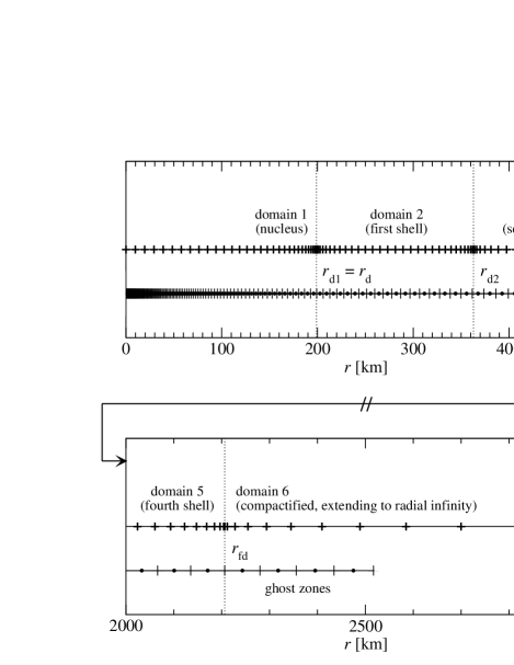
Figure 1: Radial setup of the initial spectral grid (collocation points are marked by plus symbols) and the time-independent finite difference grid (cell centers are marked by filled circles, separated by cell interfaces symbolized by vertical dashes) for a typical core collapse simulation. The upper panel shows the innermost $500{\rm\ km}$ containing the nucleus (ending at $r_{\rm d}\approx 200{\rm\ km}$), the first shell, and a part of the second shell of the spectral grid. In the lower panel a part of the last regular shell (which is confined by the outer boundary of the finite difference grid at $r_{\rm fd}\approx 2200{\rm\ km}$) and the beginning of the compactified domain of the spectral grid are plotted. The domain boundaries are indicated by vertical dotted lines.

Generally speaking, in order to achieve a comparable accuracy in the representation of functions and their derivatives, the finite difference grid needs much more points than the spectral one. For example, when considering the representation of some function like $\exp(-x^{2})$ on the interval $[0,1]$, spectral methods using Chebyshev polynomials need $\sim 30$ coefficients (and grid points) to reach machine double precision ($10^{-16}$) for the representation of the function and $10^{-13}$ for the representation of its first derivative. For comparison, a third order scheme based on finite differences needs $\sim 10^{5}$ points to achieve the same accuracy.

III.2.2 Communication between grids

Passing information from the spectral grid to the finite difference grid is technically very easy. Knowing the spectral coefficients of a function, this step simply requires the evaluation of the sum (13) at the finite difference grid points. The drawback of this method, as it will be discussed in Section IV.1, is the computational time spent. In 3D this time can even be larger than the time spent by the spectral elliptic solver. Going from the finite difference grid to the spectral grid requires an actual interpolation, taking special care to avoid Gibbs phenomena that can appear in the spectral representation of discontinuous functions. The matter terms entering in the sources of the gravitational field equations can be discontinuous when a shock forms. Thus, it is necessary to smooth or filter out high frequencies that would otherwise spoil the spectral representation. This introduces a numerical error in the fields that should remain within the overall error of the code. The important point to notice is that an accurate description needs not be achieved in the spectral representation of the sources (the hydrodynamic quantities are well described on the finite difference grid), but in that of the gravitational field, which is always continuous, as well as its first derivatives.

Technically, we interpolate from the finite difference grid to the spectral grid using a one-dimensional algorithm and intermediate grids. We first perform an interpolation in the $r$-direction, then in the $\theta$-direction and finally in the $\varphi$-direction. We can choose between piecewise linear or parabolic interpolations, and a scheme that globally minimizes the norm of the second derivative of the interpolated function novak_00_a . The filtering of spectral coefficients is performed a posteriori by removing the coefficients corresponding to higher frequencies. For example, in the radial direction, this is done by canceling the $c_{ijk}$ in Eq. (13) for $i$ larger than a given threshold. In practice, best results were found when cancelling the last third of radial coefficients. This can be linked with the so-called “two-thirds rule” used for spectral computations of quadratically nonlinear equations boyd_01_a . Nevertheless, a different (higher) threshold would also give good results, in the sense that there are no high-frequency terms rising during the metric iteration.

III.3 High-resolution shock-capturing schemes

As in our previous axisymmetric code dimmelmeier_02_a ; dimmelmeier_02_b , in the present code the numerical integration of the system of hydrodynamic equations is performed using a Godunov-type scheme. Such schemes are specifically designed to solve nonlinear hyperbolic systems of conservation laws (see, e.g. toro_97_a for general definitions and marti_03_a ; font_03_a for specific details regarding their use in special and general relativistic hydrodynamics). In a Godunov-type method the knowledge of the characteristic structure of the equations is crucial to design a solution procedure based upon either exact or approximate Riemann solvers. These solvers, which compute at every cell-interface of the numerical grid the solution of local Riemann problems, guarantee the proper capturing of all discontinuities which may appear in the flow.

The time update of the hydrodynamic equations (3) from $t^{n}$ to $t^{n+1}$ is performed using a method of lines in combination with a second-order (in time) conservative Runge–Kutta scheme. The basic conservative algorithm reads:

$$\mbox{\boldmath$U$}_{i,j,k}^{n+1}=\mbox{\boldmath$U$}_{i,j,k}^{n} - \frac{\Delta t}{\Delta r_{i}}\left(\,\widehat{\!\mbox{\boldmath$F$}}{}^{r}_{\!i+1/2,j,k}-\,\widehat{\!\mbox{\boldmath$F$}}{}^{r}_{\!i-1/2,j,k}\right)$$ (17)

$$- \frac{\Delta t}{\Delta\theta}\left(\,\widehat{\!\mbox{\boldmath$F$}}{}^{\theta}_{\!i,j+1/2,k}-\,\widehat{\!\mbox{\boldmath$F$}}{}^{\theta}_{\!i,j-1/2,k}\right)$$

$$- \frac{\Delta t}{\Delta\varphi}\left(\,\widehat{\!\mbox{\boldmath$F$}}{}^{\varphi}_{\!i,j,k+1/2}-\,\widehat{\!\mbox{\boldmath$F$}}{}^{\varphi}_{\!i,j,k-1/2}\right)$$

$$+ \Delta t\,\mbox{\boldmath$Q$}_{i,j,k}.$$

The index $n$ represents the time level, and the time and space discretization intervals are indicated by $\Delta t$ and $\Delta r_{i}$, $\Delta\theta$, and $\Delta\varphi$ for the $r$-, $\theta$-, and $\varphi$-direction, respectively. The numerical fluxes along the three coordinate directions, $\widehat{\!\mbox{\boldmath$F$}}{}^{r}$, $\widehat{\!\mbox{\boldmath$F$}}{}^{\theta}$, and $\widehat{\!\mbox{\boldmath$F$}}{}^{\varphi}$, are computed by means of Marquina’s flux formula donat_98_a . A family of local Riemann problems is set up at every cell-interface, whose jumps are minimized with the use of a piecewise parabolic reconstruction procedure (PPM) which provides third-order accuracy in space.

We note that Godunov-type schemes have also been implemented recently in 2D and 3D Cartesian codes designed to solve the coupled system of the Einstein and hydrodynamic equations, as reported in font_99_a ; font_02_a ; shibata_03_a ; baiotti_04_a .

III.4 Elliptic solvers

In the following we present the three different approaches we have implemented in our code to numerically solve the system of metric equations (11). We compare the properties of these solvers with special focus on issues like
- radius and order of convergence,
- scaling with resolution in various coordinate directions,
- imposition of boundary conditions,
- assumptions about the radial extension of the grid,
- computational performance,
- parallelization issues, and
- extensibility from two to three spatial dimensions.

In order to formalize the metric equations we define a vector of unknowns

$$\hat{u}=u^{p}=(\phi,\alpha\phi,\beta^{1},\beta^{2},\beta^{3}).$$ (18)

Then the metric equations (11) can be written as

$$\hat{f}(\hat{u})=f^{q}(u^{p})=0,$$ (19)

with $\hat{f}=f^{q}$ denoting the vector of the five metric equations for $\hat{u}$ ($p,q=1,\dots,5$). For metric solvers 1 and 2 the metric equations are discretized at cell centers $(r_{i},\theta_{j},\varphi_{k})$ on the finite difference grid. Correspondingly, for metric solver 3 the metric equations are evaluated at collocation points $(\hat{r}_{i},\hat{\theta}_{j},\hat{\varphi}_{k})$ on the spectral grid. Thus, when discretized, Eq. (19) transforms into the following coupled nonlinear system of equations of dimension $5\times n_{r}\times n_{\theta}\times n_{\varphi}$ or $5\times\hat{n}_{r}\times\hat{n}_{\theta}\times\hat{n}_{\varphi}$, respectively:

$$\mbox{\boldmath$\hat{f}$}(\mbox{\boldmath$\hat{u}$})=\hat{f}_{i,j,k}(\hat{u}_{l,m,n})=f_{i,j,k}^{q}(u_{l,m,n}^{p})=0,$$ (20)

with the vector of discretized equations $\mbox{\boldmath$\hat{f}$}=\hat{f}_{i,j,k}=f_{i,j,k}^{q}$ for the unknowns $\mbox{\boldmath$\hat{u}$}=\hat{u}_{l,m,n}=u_{l,m,n}^{p}$. For this system we have to find the roots. Note that, in general, each discretized metric equation $f_{i,j,k}^{q}$ couples both to the other metric equations through the five unknowns (indices $p$), and to other (neighboring) cell locations on the grid (indices $l,m,n$).

All three metric solvers are based on iterative methods, where the new value for the metric $\mbox{\boldmath$\hat{u}$}^{s+1}$ is computed from the value at the current iteration $s$ by adding an increment $\Delta\mbox{\boldmath$\hat{u}$}^{s}$ which is weighted with a relaxation factor $f_{\rm r}$. The tolerance measure we use to control convergence of the iteration is the maximum increment of the solution vector on the grid the iteration is executed on, i.e.

$$\Delta\hat{u}^{s}_{\rm max}=\max\,(\Delta\mbox{\boldmath$\hat{u}$}^{s})=\max\,(\Delta u_{i,j,k}^{p\,s}).$$ (21)

III.4.1 Multidimensional Newton–Raphson solver (Solver 1)

Solver 1, which was already introduced in the core collapse simulations reported in dimmelmeier_02_a ; dimmelmeier_02_b , uses a multi-dimensional Newton–Raphson iteration method to find the roots of Eq. (20). Thus, solving the nonlinear system is reduced to finding the solution of a linear problem of the same dimension during each iteration. The matrix $A$ defining the linear problem consists of the Jacobi matrix of $\hat{f}$ and additional contributions originating from boundary and symmetry conditions (see dimmelmeier_02_a for further details). As the spatial derivatives in the metric equations (which also contain mixed derivatives of second order) are approximated by second-order central differences with a three-point stencil, $A$ has a band structure with $1+2d^{2}$ bands of blocks of size $5\times 5$, where $d$ is the number of spatial dimensions of the finite difference grid. Furthermore, matrix $A$ is sparse and usually diagonally dominated.

A simple estimate already shows that the size $n\times n$ of the linear problem grows impractically large in 3D. A resolution of 100 grid points in each coordinate direction results in a square $(5\times 10^{6})\times(5\times 10^{6})$ matrix $A$. Thus, direct (exact) inversion methods, like Gauss–Jordan elimination or exact LU decomposition, are beyond practical applicability, as these are roughly $n^{3}$ processes, where $n$ is the dimension of the matrix. Even when exploiting the sparsity and band structure of $A$ the linear problem remains too large to be solved on present-day computers in a reasonable time by using iterative methods like successive over-relaxation (SOR) or conjugate gradient (CG) methods with appropriate preconditioning.

Because of these computational restrictions, the use of solver 1 is restricted to 2D axisymmetric configurations, where the matrix $A$ has nine bands of blocks. Even in this case, for coupled spacetime and hydrodynamic evolutions, the choice of linear solver methods is limited: The computational time spent by the metric solver should not exceed the time needed for one hydrodynamical time step by an excessive amount. We have found that a recursive block tridiagonal sweeping method potter_73_a (for the actual numerical implementation, see dimmelmeier_02_a ) yields the best performance for the linear problem. Here the three leftmost, middle, and rightmost bands are combined into three new bands of $n_{r}$ blocks of size $(5\times n_{\theta})\times(5\times n_{\theta})$ and which are inverted in a forward-backward recursion along the bands using a standard LU decomposition scheme for dense matrices. Actual execution times for this method and the scaling with grid resolution are given in Section IV.2.1.

We point out that the recursion method provides us with a non-iterative linear solver, and the Newton–Raphson method exhibits in general very rapid and robust convergence. Therefore, solver 1 converges rapidly to an accurate solution of the metric equations (19) even for strongly gravitating, distorted configurations, irrespective of the relative strength of the “hydrodynamics” term $S_{\rm h}$ and “metric” term $S_{\rm m}$ in the metric equations (see Eq. (12)). Its convergence radius is sufficiently large, so that even the flat Minkowski metric can be used as an initial guess for the iteration, and the relaxation factor $f_{\rm r}$ can be set equal to 1. Note that in solver 1 every metric function is treated numerically in an equal way; in particular, the equations for each of the three vector components of the shift vector $\beta^{i}$ are solved separately.

In its current implementation, solver 1 exhibits a particular disadvantage, which will be discussed in more detail in Section IV.2.2. As its spatial grid, on which the metric equations are discretized, is not radially compactified, there is a need for explicit boundary conditions of the metric functions $\hat{u}$ at the outer radial boundary of the finite difference grid. This poses a severe problem, as there exists no general analytic solution for the vacuum spacetime surrounding an arbitrary rotating fluid configuration in any coordinate system. Even in spherical symmetry, our choice of isotropic coordinates yields equations with noncompact support terms, which leads to imprecise boundary conditions, as demonstrated in Section II.2.3. Therefore, as an approximate boundary condition for an arbitrary matter configuration with gravitational mass $M_{\rm g}$, we use the monopole field for a static TOV solution,

$$\phi=1+\frac{M_{\rm g}}{2r},\qquad\alpha=\frac{1-\frac{M_{\rm g}}{2r}}{1+\frac{M_{\rm g}}{2r}},\qquad\beta^{i}=0,$$ (22)

evaluated at $r_{\rm fd}$. The influence of this approximation on the accuracy of the solution for typical compact stars is discussed in Section IV.2.2. We emphasize that the use of a noncompactified finite radial grid is not an inherent restriction of this solver method. However in the case of metric solver 1, for practical reasons we have chosen to keep the original grid setup as presented in dimmelmeier_02_a , where both the metric and hydrodynamic equations are solved on the same finite difference grid.

Finally, a further drawback of solver 1 is its inefficiency regarding scalability on parallel or vector computer architectures. The recursive nature of the linear solver part of this method prevents efficient distribution of the numerical load onto multiple processors or a vector pipeline. In combination with the disadvantageous scaling behavior of the linear solver with resolution (see also Table 3 below), these practical constraints render any extension of solver 1 to 3D beyond feasibility.

III.4.2 Conventional iterative integral nonlinear Poisson solver (Solver 2)

While solver 1 makes no particular assumption about the form of the (elliptic) equations to be solved, solver 2 exploits the fact that the metric equations (11) can be written in the form of a system of nonlinear coupled equations with a Laplace operator on the left hand side (12). A common method to solve such kind of equations is to keep the right hand side $S(\hat{u})$ fixed, solve each of the resulting decoupled linear Poisson equations, $\hat{\Delta}\hat{u}^{s+1}=S(\hat{u}^{s})$, and iterate until the convergence criterion (21) is fulfilled.

The linear Poisson equations are transformed into integral form by using a three-dimensional Green’s function,

$$\hat{u}^{s+1}(r,\theta,\varphi)=$$

$$\qquad-\frac{1}{4\pi}\!\int\!r^{\prime 2}dr^{\prime}\!\!\int\!\sin\theta^{\prime}d\theta^{\prime}\!\!\int\!d\varphi^{\prime}\,\frac{S(\hat{u}^{s}(r^{\prime},\theta^{\prime},\varphi^{\prime}))}{|\mbox{\boldmath$x$}-\mbox{\boldmath$x$}^{\prime}|},\qquad$$ (23)

where the spatial derivatives in $S$ are approximated by central finite differences. The volume integral on the right hand side of Eq. (23) is numerically evaluated by expanding the denominator into a series of radial functions $f_{l}(r,r^{\prime})$ and associated Legendre polynomials $P_{l}^{m}(\cos\theta)$, which we cut at $l=10$. The integration in Eq. (23), which has to be performed at every grid point, yields a problem of numerical size $(n_{r}\times n_{\theta}\times n_{\varphi})^{2}$. However, the problem size can be reduced to $n_{r}\times n_{\theta}\times n_{\varphi}$ by recursion. Thus, solver 2 scales linearly with the grid resolution in all spatial dimensions (see Section IV.2.1). However, while the numerical solution of an integral equation like Eq. (23) is well parallelizable, the recursive method which we employ to improve the resolution scaling performance poses a severe obstacle. In practice only the parallelization across the expansion series index $l$ (or possibly cyclic reduction) can be used to distribute the computational workload over several processors.

An advantage of solver 2 is that it does not require the imposition of explicit boundary conditions at a finite radius due to the integral form of the equations. Demanding asymptotic flatness at spatial infinity fixes the integration constants in Eq. (23). However, as the metric equations contain in general source terms with noncompact support (see Section II.2.3), the radial integration must be performed up to infinity to account for the source term contributions. As the discretization scheme used in solver 2 limits the radial integration to some finite radius $r_{\rm fd}$, the metric equations are solved only approximately if the source terms with noncompact support are nonzero. The consequences of this fact are discussed in Section IV.2.2. As in the case of metric solver 1, the metric solver 2 could be used with a compactified radial coordinate as well.

One major disadvantage of solver 2 is its slow convergence rate and a small convergence radius. For simplicity, we decompose the metric vector equation for the shift vector $\beta^{i}$ into three scalar equations for its components. If the $\theta$-component of the shift vector does not vanish, $\beta^{2}\neq 0$, and if the spacetime is nonaxisymmetric, solver 2 does not converge at all (probably due to diverging terms like $\beta^{\theta}/\sin^{2}\theta$ in the vector Laplace operator). Even when using a known solution obtained with another metric solver as initial guess, solver 2 fails to converge. Thus, the use of solver 2 is limited to axisymmetry. Even so, when $\beta^{2}\neq 0$, a quite small relaxation factor $f_{\rm r}\approx 0.05$ is required. Furthermore, as the iteration scheme is of fix-point type, it already has a much lower convergence rate than e.g. a Newton–Raphson scheme. Both factors result in typically several hundred iterations until convergence is reached (see Section IV.2.1). For strong gravity, the small convergence radius restricts the initial guess to a metric close to the actual solution of the discretized equations.

III.4.3 Iterative spectral nonlinear Poisson solver (Solver 3)

The basic principles of this iterative solver are similar to the ones used for solver 2: A numerical solution of the nonlinear elliptic system of the metric differential equations is obtained by solving the associated linear Poisson equations with a fix-point iteration procedure until convergence. However, instead of using finite difference scalar Poisson solvers, solver 3 is built from routines of the publicly available Lorene library lorene_code and uses spectral methods to solve scalar and vector Poisson equations grandclement_01_a .

Before every computation of the spacetime metric, the hydrodynamic and metric fields are interpolated from the finite difference to the spectral grid by the methods detailed in Section III.2.2. All three-dimensional functions are decomposed into Chebyshev polynomials $T_{n}(r)$ and spherical harmonics $Y_{l}^{m}(\theta,\varphi)$ in each domain. When using solver 3 the metric equations (8) are rewritten in order to gain accuracy according to the following transformations. The scalar metric functions $\phi$ and $\alpha$ have the same type of asymptotic behavior near spatial infinity, $\phi|_{r\to\infty}\sim 1+\Delta\phi(r)$, $\alpha|_{r\to\infty}\sim 1+\Delta\alpha(r)$, with $\Delta\phi(r)$ and $\Delta\alpha(r)$ approaching 0 as $r\to\infty$. Therefore, to obtain a more precise numerical description of the (usually small) deviations of $\phi$ and $\alpha$ from unity, we solve the equations for the logarithm of $\phi$ and $\alpha\phi$, imposing that $\ln\phi$ and $\ln(\alpha\phi)$ approach zero at spatial infinity. Another important difference to the other two solvers is that the vector Poisson equation for the shift vector $\beta^{i}$ is not decomposed into single scalar components, but instead the entire linear vector Poisson equation is solved, including the $\frac{1}{3}\hat{\nabla}^{i}\hat{\nabla}_{k}$ operator on the left hand side. Therefore, the system of metric equation to be solved reads

$$\begin{array}[]{rcl}\hat{\Delta}\ln\phi&=&\displaystyle-4\pi\phi^{4}\left(\rho hW^{2}-P+\frac{K_{ij}K^{ij}}{16\pi}\right)\\[6.99997pt] &&\displaystyle-\hat{\nabla}^{i}\ln\phi\;\hat{\nabla}_{i}\ln\phi,\\[6.99997pt] \hat{\Delta}\ln\alpha\phi&=&\displaystyle 2\pi\phi^{4}\left(\rho h(3W^{2}-2)+5P+\frac{7K_{ij}K^{ij}}{16\pi}\right)\!\!\!\!\!\!\!\!\!\!\!\\[6.99997pt] &&\displaystyle-\hat{\nabla}^{i}\ln\alpha\phi\;\hat{\nabla}_{i}\ln\alpha\phi,\\[6.99997pt] \hat{\Delta}\beta^{i}&+&\displaystyle\frac{1}{3}\hat{\nabla}^{i}\hat{\nabla}_{k}\beta^{k}=\displaystyle 16\pi\alpha\phi^{4}S^{i}+2\phi^{10}K^{ij}\hat{\nabla}_{j}\left(\frac{\alpha}{\phi^{6}}\right)\!.\!\!\!\!\!\!\!\!\!\!\!\!\!\!\!\!\!\end{array}$$ (24)

During each iteration a spectral representation of the solution of the linear scalar and vector Poisson equations associated with the above system is obtained. The Laplace operator is inverted (i.e. the linear Poisson equation is solved) in the following way: For a given pair of indices $l$ and $m$ of $Y_{l}^{m}(\theta,\varphi)$, the linear scalar Poisson equation reduces to an ordinary differential equation in $r$. The action of the differential operator

$$\frac{\partial^{2}}{\partial r^{2}}+\frac{2}{r}\frac{\partial}{\partial r}-\frac{l(l+1)}{r^{2}}$$ (25)

acting thus on each multipolar component ($l$ and $m$) of a scalar function corresponds to a matrix multiplication in the Chebyshev coefficient space. The corresponding matrix is inverted to obtain a particular solution in each domain, which is then combined with homogeneous solutions ($r^{l}$ and $1/r^{l}$, for a given $l$) to satisfy regularity and boundary conditions. The matrix has a small size (about $30\times 30$) and can be put into a banded form, owing to the properties of the Chebyshev polynomials, which facilitates its fast inversion. For more details about this procedure, and how the vector Poisson equation is treated, the interested reader is addressed to grandclement_01_a . Note also that when solving the shift vector equation, $\beta^{i}$ is decomposed into Cartesian components defined on the spherical polar grid (see grandclement_01_a ).

The spatial differentials in the source terms on the right hand sides of the metric equations are approximated by second-order central differences in solvers 1 and 2, while they are obtained by spectral methods in solver 3 (see Section III.2.1). When using $\sim 30$ collocation points, very high precision ($\sim 10^{-13}$) can be achieved in the evaluation of these derivatives. Another advantage of metric solver 3 is that a compactified radial coordinate $u=1/r$ enables us to solve for the entire space, and to impose exact boundary conditions at spatial infinity, $u=0$. This ensures both asymptotic flatness and fully accounts for the effects of the source terms in the metric equations with noncompact support. Solver 3 uses the same fix-point iteration method as solver 2, but does not suffer from the convergence problem encountered with that solver. Due to the direct solution of the vector Poisson equation for the shift vector $\beta^{i}$, it converges to the correct solution in all investigated models (including highly distorted 3D matter configurations with velocity perturbations, see Section IV.2.1). Furthermore, this can be achieved with the maximum possible relaxation factor, $f_{\rm r}=1$, starting from the flat metric as initial guess.

However, the strongest reason in favor of solver 3 is its straightforward extension to 3D. As mentioned previously, both metric solvers 1 and 2 are limited to axisymmetric situations. The spectral elliptic solvers provided by the Lorene library are already intrinsically three-dimensional. Indeed, even in axisymmetry the spectral grid of solver 3 requires $\hat{n}_{\varphi}=4$ grid points in the $\varphi$-direction order to correctly represent the Cartesian components of the shift vector.

There is an additional computational overhead due to the communication between the finite difference and the spectral grids. These computational costs may actually become a dominant part when calculating the metric (as will be shown in Section IV.1). The interpolation methods also have to be chosen carefully to obtain the desired accuracy. Furthermore, spectral methods may suffer from Gibbs phenomena if the source terms of the Poisson-like equations contain discontinuities. For the particular type of simulations we are aiming at, discontinuities are present (supernova shock front, discontinuity at the transition from the stellar matter distribution to the artificial atmosphere at the boundary of the star). This can result in high-frequency spurious oscillations of the metric solution, if too few radial domains are used, or if the boundaries of the spectral domains are not chosen properly. As mentioned before, a simple way to reduce the oscillations is to filter out part of the high-frequency spectral coefficients.

As the C++ routines of the Lorene library in the current release are optimized for neither vector nor parallel computers, solver 3 cannot yet exploit these architectures. However, we were able to improve the computational performance by coarse-grain parallelizing the routines which interpolate the metric solution in the spectral representation to the finite difference grid.

III.5 Extraction of gravitational waves

In a conformally flat spacetime the dynamical gravitational wave degrees of freedom are not present dimmelmeier_02_a . Therefore, in order to extract information regarding the gravitational radiation emitted in core collapse events and in rotating neutron star evolutions, we have implemented in the code the 3D generalization of the axisymmetric Newtonian quadrupole formula used in dimmelmeier_01_a ; dimmelmeier_02_a ; dimmelmeier_02_b . Note that we use spherical polar components for the tensors of the radiation field.

Whereas in axisymmetry there exists only one independent component of the quadrupole gravitational radiation field $h_{ij}^{\rm TT}$ in the transverse traceless gauge,

$$h_{ij}^{\rm TT}(r,\theta)=\frac{1}{r}A_{+}(\theta)e_{+},$$ (26)

in three dimensions we have

$$h_{ij}^{\rm TT}(r,\theta,\varphi)=\frac{1}{r}\left[A_{+}(\theta,\varphi)\mbox{\boldmath$e$}_{+}+A_{\times}(\theta,\varphi)\mbox{\boldmath$e$}_{\times}\right],$$ (27)

with the unit vectors $\mbox{\boldmath$e$}_{+}$ and $\mbox{\boldmath$e$}_{\times}$ defined as

$$\mbox{\boldmath$e$}_{+} = \mbox{\boldmath$e$}_{\theta}\otimes\mbox{\boldmath$e$}_{\theta}-\mbox{\boldmath$e$}_{\varphi}\otimes e_{\varphi},$$ (28)

$$\mbox{\boldmath$e$}_{\times} = \mbox{\boldmath$e$}_{\theta}\otimes\mbox{\boldmath$e$}_{\varphi}+\mbox{\boldmath$e$}_{\varphi}\otimes e_{\theta}.$$ (29)

The amplitudes $A_{+}$ and $A_{\times}$ are linear combinations of the second time derivative of some components of the quadrupole moment tensor $I_{ij}$, which for simplicity we evaluate at $\varphi=0$ on the polar axis and in the equatorial plane, respectively:

$$\begin{array}[]{rcl}A_{+}^{\rm p}&=&\hbox{$I_{11}$}\raise 8.26663pt\hbox{\kern-12.05553pt..}\kern 6.88889pt-\hbox{$I_{22}$}\raise 8.26663pt\hbox{\kern-12.05553pt..}\kern 6.88889pt,\\[2.5pt] A_{\times}^{\rm p}&=&2\hbox{$I_{12}$}\raise 8.26663pt\hbox{\kern-12.05553pt..}\kern 6.88889pt,\end{array} \qquad\mbox{at }\theta=0\mbox{ (pole)},$$ (32)

$$\begin{array}[]{rcl}A_{+}^{\rm e}&=&\hbox{$I_{33}$}\raise 8.26663pt\hbox{\kern-12.05553pt..}\kern 6.88889pt-\hbox{$I_{22}$}\raise 8.26663pt\hbox{\kern-12.05553pt..}\kern 6.88889pt,\\[2.5pt] A_{\times}^{\rm e}&=&-2\hbox{$I_{13}$}\raise 8.26663pt\hbox{\kern-12.05553pt..}\kern 6.88889pt,\end{array} \qquad\mbox{at }\theta=\pi/2\mbox{ (equator)}.$$ (35)

A direct numerical calculation of the quadrupole moment in the standard quadrupole formulation,

$$I_{ij}=\!\!\int\!dV\rho^{*}\!\left[x_{i}x_{j}-\frac{1}{3}\delta_{ij}\left(x_{1}^{2}+x_{2}^{2}+x_{3}^{2}\right)\right]\!,$$ (36)

results in high frequency noise completely dominating the wave signal due to the presence of the second time derivatives in Eq. (35). Therefore, we make use of the time-differentiated quadrupole moment in the first moment of momentum density formulation,

$$\dot{I}_{ij}=\!\!\int\!dV\rho^{*}\!\left[v_{i}x_{j}+v_{j}x_{i}-\frac{2}{3}\delta_{ij}\left(v_{1}x_{1}+v_{2}x_{2}+v_{3}x_{3}\right)\right]\!,$$ (37)

and stress formulation,

$$\hbox{$I_{ij}$}\raise 8.26663pt\hbox{\kern-10.54855pt..}\kern 5.16663pt=\!\!\int\!dV\rho^{*}\left[2v_{i}v_{j}-x_{i}\partial_{j}\Phi-x_{j}\partial_{i}\Phi\right]\!,$$ (38)

of the quadrupole formula finn_89_a ; blanchet_90_a .

In the above equations, $x_{i}$ and $v_{i}$ are the coordinates and velocities in Cartesian coordinates, respectively. When evaluating Eq. (38) numerically, we transform $v_{i}$ to spherical polar coordinates. In the quadrupole moment, we use $\rho^{*}=\rho W\phi^{6}$ instead of $\rho$ as in dimmelmeier_01_a ; dimmelmeier_02_a ; dimmelmeier_02_b , as this quantity is evolved by the continuity equation (note that both quantities have the same Newtonian limit). This also allows a direct comparison with the results presented in shibata_03_b , which we show in Section IV.2.4. For a discussion about the ambiguities arising from the spatial derivatives of the Newtonian potential $\Phi$ in Eq. (38) in a general relativistic framework and their solution (which we also employ in this work), we refer to dimmelmeier_02_b .

The total energy emitted by gravitational waves can be expressed either as a time integral,

$$E_{\rm gw} = \frac{2}{15}\int dt\biggl{[}-\hbox{$I_{11}$}\raise 8.26663pt\hbox{\kern-13.56242pt...}\kern 5.16663pt\hbox{$I_{22}$}\raise 8.26663pt\hbox{\kern-13.56242pt...}\kern 5.16663pt-\hbox{$I_{11}$}\raise 8.26663pt\hbox{\kern-13.56242pt...}\kern 5.16663pt\hbox{$I_{33}$}\raise 8.26663pt\hbox{\kern-13.56242pt...}\kern 5.16663pt-\hbox{$I_{22}$}\raise 8.26663pt\hbox{\kern-13.56242pt...}\kern 5.16663pt\hbox{$I_{33}$}\raise 8.26663pt\hbox{\kern-13.56242pt...}\kern 5.16663pt$$ (39)

$$+\hbox{$I_{11}$}\raise 8.26663pt\hbox{\kern-13.56242pt...}^{2}\kern 0.86108pt+\hbox{$I_{22}$}\raise 8.26663pt\hbox{\kern-13.56242pt...}^{2}\kern 0.86108pt+\hbox{$I_{33}$}\raise 8.26663pt\hbox{\kern-13.56242pt...}^{2}\kern 0.86108pt+3\left(\hbox{$I_{12}$}\raise 8.26663pt\hbox{\kern-13.56242pt...}^{2}\kern 0.86108pt+\hbox{$I_{13}$}\raise 8.26663pt\hbox{\kern-13.56242pt...}^{2}\kern 0.86108pt+\hbox{$I_{23}$}\raise 8.26663pt\hbox{\kern-13.56242pt...}^{2}\kern 0.86108pt\right)\biggr{]},\quad$$

or, equivalently, as a frequency integral,

$$E_{\rm gw} = \frac{1}{15}\int\nu^{2}d\nu\biggl{[}-\hbox{$I_{11}$}\raise 2.58334pt\hbox{\kern-10.76385pt$\hat{\dot{}\kern 3.01385pt\dot{}}$}\kern 7.74998pt\hbox{$I_{22}$}\raise 2.58334pt\hbox{\kern-10.76385pt$\hat{\dot{}\kern 3.01385pt\dot{}}$}\kern 7.74998pt-\hbox{$I_{11}$}\raise 2.58334pt\hbox{\kern-10.76385pt$\hat{\dot{}\kern 3.01385pt\dot{}}$}\kern 7.74998pt\hbox{$I_{33}$}\raise 2.58334pt\hbox{\kern-10.76385pt$\hat{\dot{}\kern 3.01385pt\dot{}}$}\kern 7.74998pt-\hbox{$I_{22}$}\raise 2.58334pt\hbox{\kern-10.76385pt$\hat{\dot{}\kern 3.01385pt\dot{}}$}\kern 7.74998pt\hbox{$I_{33}$}\raise 2.58334pt\hbox{\kern-10.76385pt$\hat{\dot{}\kern 3.01385pt\dot{}}$}\kern 7.74998pt$$ (40)

$$+\hbox{$I_{11}$}\raise 2.58334pt\hbox{\kern-10.76385pt$\hat{\dot{}\kern 3.01385pt\dot{}}$}^{\,2}\kern 2.15277pt+\hbox{$I_{22}$}\raise 2.58334pt\hbox{\kern-10.76385pt$\hat{\dot{}\kern 3.01385pt\dot{}}$}^{\,2}\kern 2.15277pt+\hbox{$I_{33}$}\raise 2.58334pt\hbox{\kern-10.76385pt$\hat{\dot{}\kern 3.01385pt\dot{}}$}^{\,2}\kern 2.15277pt+3\left(\hbox{$I_{12}$}\raise 2.58334pt\hbox{\kern-10.76385pt$\hat{\dot{}\kern 3.01385pt\dot{}}$}^{\,2}\kern 2.15277pt+\hbox{$I_{13}$}\raise 2.58334pt\hbox{\kern-10.76385pt$\hat{\dot{}\kern 3.01385pt\dot{}}$}^{\,2}\kern 2.15277pt+\hbox{$I_{23}$}\raise 2.58334pt\hbox{\kern-10.76385pt$\hat{\dot{}\kern 3.01385pt\dot{}}$}^{\,2}\kern 2.15277pt\right)\biggr{]},\qquad$$

where $\hbox{$I_{ij}$}\raise 2.58334pt\hbox{\kern-9.47217pt$\hat{\dot{}\kern 3.01385pt\dot{}}$}\kern 6.45831pt(\nu)$ is the Fourier transform of $\hbox{$I_{ij}$}\raise 8.26663pt\hbox{\kern-10.54855pt..}\kern 5.16663pt(t)$. We point out that the above general expressions reduce to the following ones in axisymmetry:

$$A_{+}^{\rm p}=0,\qquad A_{\times}^{\rm p}=0,\qquad A_{+}^{\rm e}=\hbox{$I$}\raise 8.26663pt\hbox{\kern-4.30554pt..},\qquad A_{\times}^{\rm e}=0,$$ (41)

$$\displaystyle E_{\rm gw}=\frac{2}{15}\int dt\,\hbox{$I$}\raise 8.26663pt\hbox{\kern-5.8125pt...}^{2}=\frac{1}{15}\int\nu^{2}d\nu\,\hbox{$I$}\raise 2.58334pt\hbox{\kern-3.01385pt$\hat{\dot{}\kern 3.01385pt\dot{}}$}^{\,2}\kern-2.15277pt,$$ (42)

with $I=I_{33}-I_{22}$ being the only nonzero independent component of the quadrupole tensor, and $\hbox{$I$}\raise 2.58334pt\hbox{\kern-3.01385pt$\hat{\dot{}\kern 3.01385pt\dot{}}$}^{\,2}\kern-2.15277pt$ being the Fourier transform of $\hbox{$I$}\raise 8.26663pt\hbox{\kern-4.52083pt..}^{2}\kern-1.29167pt$. The quadrupole wave amplitude $A^{\rm E2}_{20}$ used in zwerger_97_a ; dimmelmeier_01_a ; dimmelmeier_02_b is related to $I$ according to $A^{\rm E2}_{20}=8\sqrt{\pi/15}\,\hbox{$I$}\raise 8.26663pt\hbox{\kern-4.30554pt..}$.

We have tested the equivalence between the waveforms obtained by the axisymmetric code presented in dimmelmeier_01_a ; dimmelmeier_02_a ; dimmelmeier_02_b and those by the current three-dimensional code using the corresponding axisymmetric model. In all investigated cases, they agree with excellent precision.

IV Code tests and applications

We turn now to an assessment of the numerical code with a variety of tests and applications. We recall that we do not attempt in the present paper to investigate any realistic astrophysical scenario, which is deferred to subsequent publications. Instead, we focus here on discussing standard tests for general relativistic three-dimensional hydrodynamics code, which were all passed by our code. In particular, we show that the code exhibits long-term stability when evolving strongly gravitating systems like rotational core collapse and equilibrium configurations of (highly perturbed) rotating relativistic stars. Each separate constituent methods of the code (HRSC schemes for the hydrodynamics equations and elliptic solvers based on spectral methods for the gravitational field equations) has already been thoroughly tested and successfully applied in the past (see e.g. font_03_a ; marti_03_a ; grandclement_01_a and references therein). Therefore, we mainly demonstrate here that the coupled numerical schemes work together as desired.

IV.1 Interpolation efficiency and accuracy

Table 1: Execution time $t_{\rm fd\rightarrow sp}$ and accuracy $\Delta f_{\rm fd\rightarrow sp}$ for the interpolation of a test function $f_{\rm t}(r,\theta,\varphi)$ (see text) from the finite difference grid to the spectral grid, listed for different finite difference grid resolutions $n_{r}\times n_{\theta}\times n_{\varphi}$ and interpolation types. The interpolation methods are piecewise linear (type 1), piecewise parabolic (type 2), and globally minimizing the norm of the second derivative of the interpolated function novak_00_a (type 0). The spectral grid has a resolution of $\hat{n}_{r}=17$, $\hat{n}_{\theta}=17$, and $\hat{n}_{\varphi}=16$ grid points.

$n_{r}\times n_{\theta}\times n_{\varphi}$	Type	$t_{\rm fd\rightarrow sp}$ [s]	$\Delta f_{\rm fd\rightarrow sp}$ [$L_{0}$ norm]
$400\times 200\times 800$	2	5.13	$5.0\times 10^{-8}$
$400\times 200\times 800$	1	5.12	$7.0\times 10^{-6}$
$400\times 200\times 800$	0	9.44	$1.8\times 10^{-6}$
$400\times 200\times 400$	2	2.92	$3.1\times 10^{-7}$
$400\times 200\times 200$	2	1.43	$1.6\times 10^{-6}$
$400\times 200\times 100$	2	0.77	$1.7\times 10^{-5}$
$400\times 200\times\hskip 5.00002pt10$	2	0.09	$1.3\times 10^{-2}$
$400\times 100\times 800$	2	2.55	$3.1\times 10^{-7}$
$400\times\hskip 5.00002pt50\times 800$	2	1.60	$1.8\times 10^{-6}$
$400\times\hskip 5.00002pt\hskip 5.00002pt5\times 800$	2	0.32	$2.0\times 10^{-3}$
$200\times 200\times 800$	2	3.61	$2.7\times 10^{-7}$
$100\times 200\times 800$	2	1.81	$2.1\times 10^{-6}$
$\hskip 5.00002pt50\times 200\times 800$	2	1.40	$1.6\times 10^{-5}$
$\hskip 5.00002pt\hskip 5.00002pt5\times 200\times 800$	2	0.99	$1.4\times 10^{-2}$

The interpolation procedure from the finite difference grid to the spectral grid has been described in Section III.2.2. Among the three possible algorithms we have implemented in the code, the most efficient turned out to be the one based on a piecewise parabolic interpolation (see Table 1). It is as fast as the piecewise linear interpolation, and more accurate than the algorithm based on the minimization of the second derivative of the interpolated function. Table 1 shows, for a particular example of an interpolated test function $f_{\rm t}(r,\theta,\varphi)=\exp\left[-r^{2}(1+\sin^{2}\theta\cos^{2}\varphi)\right]$, the relative accuracy $\Delta f_{\rm int}$ (in the $L_{0}$ norm) achieved by this interpolation, as well as the CPU time spent on a Pentium IV Xeon processor at 2.2 GHz. The spectral grid consists of two domains (nucleus + shell) with $\hat{n}_{r}=17$, $\hat{n}_{\theta}=17$, and $\hat{n}_{\varphi}=16$. The outer radius of the nucleus is located at 0.5, and the outer boundary of the shell is at 1.5 (corresponding to the radius of the finite difference grid $r_{\rm fd}$).

This test demonstrates that the piecewise parabolic interpolation is indeed third-order accurate, and that the time spent scales roughly linearly with the number of points of the finite difference grid in any direction. We have made other tests which show that the interpolation accuracy is independent of $\hat{n}$, and that it scales in time like ${\cal O}\left(\hat{n}^{3}\right)+{\cal O}\left(n^{3}\right)$, where $\hat{n}$ and $n$ are the number of points used in each dimension by the spectral and the finite difference grid, respectively. The interpolation is exact, up to machine precision, for functions which can be expressed as polynomials of degree $\leq 2$ with respect to all three coordinates.

Table 2: Execution time $t_{\rm sp\rightarrow fd}$ and accuracy $\Delta f_{\rm sp\rightarrow fd}$ for the evaluation of a test function $f_{\rm t}(r,\theta,\varphi)$ (see text) on the finite difference grid from its representation in spectral coefficients, listed for different numbers of spectral grid points $\hat{n}_{r}\times\hat{n}_{\theta}\times\hat{n}_{\varphi}$. The finite difference grid has a resolution of $n_{r}=100$, $n_{\theta}=50$, and $n_{\varphi}=30$ grid points.

$\hat{n}_{r}\times\hat{n}_{\theta}\times\hat{n}_{\varphi}$	$t_{\rm sp\rightarrow fd}$ [s]	$\Delta f_{\rm sp\rightarrow fd}$ [$L_{0}$ norm]
$33\times 17\times 64$	75.8	$1.5\times 10^{-15}$
$33\times 17\times 32$	38.4	$5.5\times 10^{-9\hskip 3.5pt}$
$33\times 17\times 16$	19.6	$2.6\times 10^{-4\hskip 3.5pt}$
$33\times 17\times\hskip 5.00002pt8$	10.3	$2.8\times 10^{-2\hskip 3.5pt}$
$33\times\hskip 5.00002pt9\times 64$	40.8	$6.4\times 10^{-9\hskip 3.5pt}$
$33\times\hskip 5.00002pt5\times 64$	23.4	$3.2\times 10^{-4\hskip 3.5pt}$
$17\times 17\times 64$	41.2	$1.9\times 10^{-13}$
$\hskip 5.00002pt9\times 17\times 64$	24.6	$9.2\times 10^{-7\hskip 3.5pt}$
$\hskip 5.00002pt5\times 17\times 64$	16.7	$1.9\times 10^{-3\hskip 3.5pt}$

The direct spectral summation from the spectral to the finite difference grid is a very precise way of evaluating a function: For smooth functions, the relative error decreases like $\exp({-\hat{n}})$ (infinite order scheme). This property is fulfilled in our code, as shown in Table 2 for the same test function $f_{\rm t}(r,\theta,\varphi)$ and the same domain setup as for Table 1 (again the timings are for a Pentium IV Xeon processor at 2.2 GHz). Double precision accuracy is reached with a reasonable number of points ($\hat{n}_{r}=33$, $\hat{n}_{\theta}=17$, and $\hat{n}_{\varphi}=64$). According to Table 2 the CPU cost scales linearly with the number of coefficients $\hat{n}$ in any direction. We have also confirmed that it scales linearly with the number of finite difference grid points $n$ in any direction. The drawback of this most straightforward procedure is that it requires ${\cal O}\left(\hat{n}^{3}n^{3}\right)$ operations, which is much more expensive than the interpolation from the finite difference grid to the spectral one, and even more expensive than the iterative procedure providing the solution of system (24). Nevertheless, it is computationally not prohibitive since the overall accuracy of the code does not depend on $\hat{n}$ (which can thus remain small). A way to reduce the execution time is to use a partial summation algorithm (see e.g. boyd_01_a ), which needs only ${\cal O}\left(\hat{n}n^{3}\right)+{\cal O}\left(\hat{n}^{2}n^{2}\right)+{\cal O}\left(\hat{n}^{3}n\right)$ operations, at the additional cost of increased central memory requirement. Another alternative is to truncate the spectral sum, staying at an accuracy level comparable to that of finite difference differential operators.

IV.2 Solver comparison in 2D

IV.2.1 Convergence properties

The theoretical considerations about the convergence properties of the three implemented metric solvers (as outlined in Section III.4) are checked by solving the spacetime metric for a 2D axisymmetric rotating neutron star model in equilibrium (labeled model RNS), which we have constructed with the method described in Komatsu et al. komatsu_89_a . This model has a central density $\rho_{\rm c}=7.905\times 10^{14}{\rm\ g\ cm}^{-3}$, obeys a polytropic EoS with $\gamma=2$ and $K=1.455\times 10^{5}$ (in cgs units), and rotates rigidly at the mass shedding limit, which corresponds to a polar-to-equatorial axis ratio of 0.65. These model parameters are equivalent to those used for neutron star models in font_00_a ; font_02_a .

Figure 2: Comparison of the convergence behavior for the three metric solvers in 2D. For solver 1 (filled circles), the maximum increment $\Delta\hat{u}^{s}_{\rm max}$ per iteration $s$ decreases to the threshold $\Delta\hat{u}^{s}_{\rm thr}=10^{-15}$ (lower horizontal dotted line) within less than 10 iterations, while solver 3 (asterisks) needs more than 40 iterations to reach its (less restrictive) threshold (upper horizontal dotted line) of $10^{-6}$. The very low relaxation factor needed for solver 2 (filled squares) results in a remarkably slow convergence, requiring more than 700 iterations. The solid lines mark the approximate linear decrease of $\log\Delta\hat{u}^{s}_{\rm max}$.

To the initial equilibrium model we add an $r$- and $\theta$-dependent density and velocity perturbation,

$$\begin{array}[]{rcl}\rho&=&\displaystyle\rho_{\rm ini}\left[1+0.02\sin^{2}\!\left(\!\pi\frac{r}{r_{\rm s}}\right)\left(1+\sin^{2}(2\theta)\right)\right],\\[10.00002pt] v_{r}&=&\displaystyle 0.05\sin^{2}\!\left(\!\pi\frac{r}{r_{\rm s}}\right)\left(1+\sin^{2}(2\theta)\right),\\[10.00002pt] v_{\theta}&=&\displaystyle 0.05\sin^{2}\!\left(\!\pi\frac{r}{r_{\rm s}}\right)\sin^{2}(2\theta),\\[10.00002pt] v_{\varphi}&=&\displaystyle v_{\varphi\,\rm ini}+0.05\sin^{2}\!\left(\!\pi\frac{r}{r_{\rm s}}\right)\left(1+\sin^{2}(2\theta)\right),\end{array}$$ (43)

where $r_{\rm s}$ is the ($\theta$-dependent) stellar radius, and $v_{r}=\sqrt{v_{1}v^{1}}$, $v_{\theta}=\sqrt{v_{2}v^{2}}$, and $v_{\varphi}=\sqrt{v_{3}v^{3}}$. The metric equations (Eqs. (11) for solvers 1 and 2, and Eqs. (24) in the case of solver 3) are then solved using the three implemented metric solvers. The perturbation of $v_{r}$ and $v_{\theta}$ ensures that the metric equations yield the general case of a shift vector with three nonzero components, which cannot be obtained with an initial model in equilibrium.

We point out that by adding the perturbations specified in Eq. (43) and calculating the metric for these perturbed initial data, we add a small inconsistency to the initial value problem. As the Lorentz factor $W$ in the right hand sides of the metric equations contains metric contributions (which are needed for computing the covariant velocity components), it would have to be iterated with the metric solution until convergence. However, as the perturbation amplitude is small, and as we do not evolve the perturbed initial data, we neglect this small inconsistency.

The most relevant quantity related to convergence properties of the metric solver is the maximum increment $\Delta\hat{u}^{s}_{\rm max}$ of all metric components on the grid (see Fig. 2). As expected solver 1 exhibits the typical quadratic decline of a Newton–Raphson solver to its threshold value $\Delta\hat{u}^{s}_{\rm thr}=10^{-15}$. As the methods implemented in solvers 2 and 3 correspond to a fix-point iteration, the decline of their metric increment is significantly slower. Therefore, for the Poisson-based solvers, we typically use a less restrictive threshold $\Delta\hat{u}^{s}_{\rm thr}=10^{-6}$. While the spectral Poisson solver 3 allows for a relaxation factor of 1 and thus for a still quite rapid convergence, the conventional Poisson solver 2 requires more than 700 iterations due to its much smaller relaxation factor imposed by the $\beta^{2}$-equation.

It is worth stressing that all three solvers show rather robust convergence, if one keeps in mind that the initial guess is the flat spacetime metric. If the metric is changing dynamically during an evolution, the metric values from the previous computation can be used as new starting values, which reduces the number of iterations by about a factor of two with respect to those reported in Fig. 2.

Besides the convergence rate, the execution time $t_{\rm m}$ required for a single metric computation and its dependence on the grid resolution is also of paramount relevance for the practical usefulness of a solver. These times for one metric computation of the perturbed RNS stellar model on a finite difference grid with various $r$- and $\theta$-resolutions on an IBM RS/6000 Power4 processor are summarized in Table 3. As theoretically expected, both solver 1 and 2 show a linear scaling of $t_{\rm m}$ with the number of radial grid points $n_{r}$, i.e. the ratio $r_{n_{r}}=t_{\rm m}(n_{r})/t_{\rm m}(n_{r/2})$ is approximately 2. While the integration method of solver 2 shows linear dependence also for the number of meridional grid zones $n_{\theta}$, the inversion of the dense $n_{\theta}\times n_{\theta}$ matrices during the radial sweeps in solver 1 is roughly a $n_{\theta}^{3}$ process. Thus, the theoretical value of $r_{n_{\theta}}=8$ for that solver is well met by the results shown in Table 3. We note that for even larger values of $n_{\theta}$, specific processor properties like cache-miss problems can even worsen the already cubic scaling of solver 1, while for $n_{\theta}\gtrsim 64$ solver 2 fails to converge altogether. On the other hand for solver 3 $t_{\rm m}$ is approximately independent of the number of finite difference grid points in either coordinate direction, as the number of spectral collocation points is fixed. A dependence on $n_{r}$ and $n_{\theta}$ can only enter via the interpolation procedure between the two grids, the time for which is, however, entirely negligible in 2D.

Table 3: Metric solver execution time $t_{\rm m}$ for different finite difference grid resolutions $n_{r}\times n_{\theta}$ for the three metric solvers in 2D applied to the perturbed rotating neutron star model RNS. The ratios $a_{n_{r}}$ ($a_{n_{\theta}}$) between execution times for a given $n_{r}$ ($n_{\theta}$) and for half that resolution exhibit the behavior expected from theoretical considerations. The spectral grid has a resolution of $\hat{n}_{r}=33$, $\hat{n}_{\theta}=17$, and $\hat{n}_{\varphi}=4$ grid points.

	Solver 1			Solver 2			Solver 3
$n_{r}\times n_{\theta}$	$t_{\rm m}$ [s]	$a_{n_{r}}$	$a_{n_{\theta}}$	$t_{\rm m}$ [s]	$a_{n_{r}}$	$a_{n_{\theta}}$	$t_{\rm m}$ [s]	$a_{n_{r}}$	$a_{n_{\theta}}$
$\hskip 5.00002pt50\times 16$	1.8			2.8			20.7
$100\times 16$	3.7	2.0		5.9	2.1		20.6	1.0
$200\times 16$	7.4	2.0		12.9	2.2		20.8	1.0
$\hskip 5.00002pt50\times 32$	12.5		6.9	5.9		2.1	20.8		1.0
$100\times 32$	25.4	2.0	6.9	12.3	2.1	2.1	20.5	1.0	1.0
$200\times 32$	50.8	2.0	6.9	27.1	2.2	2.1	21.7	1.1	1.0
$\hskip 5.00002pt50\times 64$	109.7		8.8	12.4		2.1	20.9		1.0
$100\times 64$	224.2	2.0	8.8	–			21.5	1.0	1.1
$200\times 64$	445.2	2.0	8.8	–			21.7	1.0	1.1

The break even point for the three solvers corresponds roughly to a resolution of $100\times 32$ grid points at $t_{\rm m}\sim 20{\rm\ s}$. We emphasize that this value of $t_{\rm m}$ is much larger than the time needed for one hydrodynamic step at the same resolution, which is roughly $t_{\rm h}\sim 0.1{\rm\ s}$. From the results reported in Table 3 it becomes evident that due to the independence of $t_{\rm m}$ on the finite difference grid resolution in the spectral metric solver 3, this method is far superior to the other two solvers for simulations requiring a large number of grid points in general, and particularly in $\theta$-direction.

IV.2.2 Radial fall-off of the metric components

When comparing in Section III.4 the theoretical foundations of the three alternative metric solvers implemented in the code, we already raised the issue of the existence of source terms with noncompact support in the metric equations (11) (see Section II.2.3). Neither the Newton–Raphson-based solver 1, which requires explicit boundary conditions at the finite radius $r_{\rm fd}$ (which are in general not exactly known and possibly time-dependent), nor the conventional iterative Poisson solver 2, which integrates the Poisson-like metric equations only up to the same finite radius $r_{\rm fd}$, are able to fully account for the nonlinear source terms, even if the radial boundary of the finite difference grid is in the vacuum region outside the star, $r_{\rm fd}>r_{\rm s}$.

Hence, both solvers yield a numerical solution of the exact metric equations only in very few trivial cases, like e.g. the solution for the metric of a spherically symmetric static matter distribution (TOV solution), when the metric equations reduce to Poisson-like equations with compact support. However, due to the radial compactification of the spectral grid, which allows for the Poisson equations to be numerically integrated out to spacelike infinity, the spectral solver 3 can consistently handle all noncompact support source terms in the metric equations in a non-approximative way. This property holds even when the metric quantities are mapped from the spectral grid onto the finite difference grid, the latter extending only to $r_{\rm fd}$. Thus, we expect that only solver 3 captures the correct radial fall-off behavior of the metric quantities outside the matter distribution.

Figure 3: Equatorial profile of the shift vector component $\beta_{\varphi\rm\,e}$ obtained by different metric solvers compared with the correct profile from the initial data solver (solid line) for the rotating neutron star model RNS. Due to its approximate boundary value, the profile from solver 1 (dashed line) shows large deviation from the correct solution, particularly for a grid boundary $r_{\rm fd}$ close to the stellar equatorial radius $r_{\rm s\,e}$ (upper panel). As solver 2 (dashed-dotted line) needs no explicit boundary conditions, its solution matches well with the correct solution, with improving agreement as $r_{\rm fd}$ is at larger distance from $r_{\rm s\,e}$ (lower panel). The compactified radial grid of solver 3 (dotted line) fully accounts for non-compact support terms, and thus agrees very well with the correct solution, independent of the location of $r_{\rm fd}$. The radii $r_{\rm s\,e}$ and $r_{\rm fd}$ are indicated by vertical dotted lines.

In the following we illustrate the effects of noncompact support terms in the metric equations on the numerical solution using the three different solvers. Fig. 3 shows the radial equatorial profiles of the rotational shift vector component $\beta_{\varphi}=\sqrt{\gamma_{33}}\beta^{3}$ for the rapidly rotating neutron star initial model (RNS) specified in Section IV.2.1, obtained with the three alternative metric solvers. While we restrict our discussion to the particular metric quantity $\beta_{\varphi{\rm\,e}}$ we notice that the radial fall-off behavior and the dependence on the solver method is equivalent for all other metric components.

In the upper panel of Fig. 3 the equatorial stellar boundary $r_{\rm s\,e}$ is very close to the radial outer boundary of the finite difference grid, $r_{\rm s\,e}=0.9\,r_{\rm fd}$ (both indicated by vertical dotted lines). The star and the exterior atmosphere are resolved using $n_{r{\rm\,s}}=90$ radial grid points for the star and $n_{r{\rm\,a}}=10$ radial grid points for the atmosphere (along the equator), respectively, and $n_{\theta}=30$ meridional points. The spectral solver 3 uses $\hat{n}_{r}=33$ radial and $\hat{n}_{\theta}=17$ meridional grid points.

If the boundary value for the metric at $r_{\rm fd}$ is exact, solver 1 always yields the correct solution, irrespective of the source terms not having compact support. For stationary solutions like rotating neutron stars these exact values can in principle be provided by the initial data solver. However, for instance in a dynamical situation, exact values cannot be provided, and we are forced to use approximate boundary conditions, which we choose according to Eq. (22). As the approximate boundary value for solver 1, $\beta_{\varphi}(r_{\rm fd})=0$, is far from the exact value, the corresponding profile of the shift vector (dashed line) strongly deviates from the correct $\beta_{\varphi{\rm\,e}}$ obtained by the initial data solver (solid line). Note that the exact solution is given only for $r\leq r_{\rm s\,e}$, due to limitations of the initial solver method komatsu_89_a . As shown in the lower panel of the figure, with increasing distance of the finite difference grid boundary from the stellar boundary ($r_{\rm fd}=2.0\,r_{\rm s\,e}$ with $n_{r{\rm\,s}}=n_{r{\rm\,a}}=90$), the approximation for $\beta_{\varphi{\rm\,e}}(r_{\rm fd})$ improves noticeably, and so does the matching of $\beta_{\varphi{\rm\,e}}$ with the correct solution.

On the other hand, as the integral approach of solvers 2 and 3 requires no specific boundary conditions at a finite radius (contrary to solver 1), the numerical solution for $\beta_{\varphi{\rm\,e}}$ agrees well with the correct solution even for an integration boundary $r_{\rm fd}$ close to the stellar boundary $r_{\rm s\,e}$ (dashed-dotted and dotted lines in Fig. 3, respectively). For $r_{\rm fd}\gg r_{\rm s\,e}$, when the influence of the source terms with noncompact support is increasingly picked up by the radial integral, the solutions supplied by solver 2 rapidly approach the correct one. The terms with noncompact support usually do not contribute strongly to the solution of the metric equations (except in cases of very strong gravity and extremely rapid contraction or rotation). Thus, solver 2 is superior to solver 1 when approximate boundary values must be used, Eq. (22). Solver 3, on the other hand, has the key advantage over solver 2 of using very accurate spectral methods for solving the Poisson equation over the entire spatial volume due to its compactified radial coordinate. Hence, irrespective of the distance of $r_{\rm fd}$ from $r_{\rm s\,e}$, it yields the same results on the finite difference grid, onto which the results are mapped from the spectral grid.

The (small) difference between the results for $\beta_{\varphi{\rm\,e}}$ from solver 3 and from the initial data solver is partly due to the accuracy of the numerical schemes and the mapping between different grids, and particularly a result of the CFC approximation of the field equations employed by the evolution code (note that the initial data are generated from a numerical solution of the exact Einstein metric equations). In the case of rapidly rotating neutron star models we have found that the truncation error and the error arising from the mapping of the initial data to the evolution code is typically more than one order of magnitude smaller than the error which can be attributed to the CFC approximation, if a grid with a resolution $n_{r}\sim 100$, $n_{\theta}\sim 30$ and $\hat{n}_{r}=33$, $\hat{n}_{\theta}=17$ is used. For estimates of the quality of the CFC approximation in such cases, see dimmelmeier_02_a and references therein.

We again note that, in principle, the use of a compactified radial grid is not confined to the spectral solver 3. A finite difference grid extending to spatial infinity could be used for solvers 1 and 2 as well. However, in that case either the exterior atmosphere would also have to be extended to the entire grid too (generating unnecessary computations), or only the relevant portion of the grid containing the star would have to be evolved in time (creating an additional boundary). When using solver 3, there is a clearcut split between the finite difference grid and the spectral grid. Thus, the hydrodynamic quantities can be defined on a grid with an atmosphere of only small size, while the metric in the compactified domain can be computed very accurately with only few radial collocation points due to the exponential convergence of spectral methods in this smooth region. Additionally, the Lorene library provides the use of a compactified radial domain as an already implemented option at no extra cost.

IV.2.3 Axisymmetric core collapse to a neutron star –
Construction of the spectral grid domains

As all three metric solvers yield equally precise numerical solutions of the spacetime metric in 2D, they give nearly identical results when applied to simulations of rotational core collapse, as shown in Fig. 4. For the results presented in this figure we have chosen the stellar core collapse model labeled A3B2G4 in dimmelmeier_02_b (model SCC in the following), which rotates differentially and moderately fast, and has an initial central density $\rho_{\rm c}=10^{10}{\rm\ g\ cm}^{-3}$. The initial adiabatic index is reduced from $\gamma_{\rm i}=4/3$ to $\gamma_{1}=1.3$ during contraction, and is increased to $\gamma_{2}=2.5$ beyond supranuclear matter densities, $\rho>\rho_{\rm nuc}=2.0\times 10^{14}{\rm\ g\ cm}^{-3}$. The details of the EoS for this model are given by Eq. (6). As the metric calculation is computationally very expensive, it is done only every 100/10/50 hydrodynamic time steps before/during/after core bounce, and extrapolated in between (for details on the satisfactory accuracy of this procedure see dimmelmeier_02_a ). The number of zones used in the finite difference grid is $n_{r}=200$ and $n_{\theta}=30$, with logarithmic spacing in the $r$-direction and a central resolution of 500 m, and an equidistant spacing in the $\theta$-direction. Again, the grid resolution of the spectral solver 3 is $\hat{n}_{r}=33$ and $\hat{n}_{\theta}=17$.

Figure 4: Time evolution of the central conformal factor $\phi_{\rm c}$ (upper panel) for the core collapse model SCC, using metric solver 1 (solid line), 2 (dashed line), and 3 (dashed-dotted line), respectively. All three solvers yield similar results. The small relative differences of less than $10^{-3}$ in $\phi_{\rm c}$ (lower panel) obtained with solvers 1 and 3 (solid line) and solver 2 and 3 (dashed line) prove that numerical variations of the metric from each solver are of the order of the small overall discretization error of the entire evolution code. The time of bounce $t_{\rm b}$ is indicated by the vertical dotted line.

In the upper panel of Fig. 4 we plot the time evolution of the central conformal factor $\phi_{\rm c}$, which rises steeply when the central density increases to supranuclear densities, reaches a maximum at the time of core bounce $t_{\rm b}$ (vertical dotted line), and subsequently approaches a new equilibrium value with decreasing ringdown oscillations. This new state, which is reached asymptotically, signals the formation of a pulsating compact remnant which can be identified with the nascent proto-neutron star. Each of the three curves in this upper panel is the result of using one of the three available metric solver (see caption for details). The lower panel of the figure demonstrates that the relative differences found in the dynamical evolution of our representative core collapse model are negligibly small when using either metric solver, which proves the applicability of any of the metric solvers in 2D.

Figure 5: Two different methods for determining the domain radii of the spectral grid boundary. The upper panel shows the time evolution of the domain radius parameter $r_{\rm d}$ for the core collapse model SCC, where $r_{\rm d}$ is either set by the sonic point method (solid line; sonic point first detected at $t\sim 23{\rm\ ms}$) or by the rest mass fraction method (dashed line). The boundary of the finite difference grid $r_{\rm fd}$, the stellar equatorial radius $r_{\rm s\,e}$, the minimal domain radius $r_{\rm d\,min}$ (set to $r_{40}$), and the approximate location of shock formation $r_{\rm sh}$ are indicated by horizontal dotted lines. The relative difference between the values of $\phi_{\rm c}$ from simulations using the two methods (lower panel) is less than $10^{-4}$ throughout the evolution. The time of bounce $t_{\rm b}$ is indicated by the vertical dotted line.

However, in such a highly dynamical situation, where the relevant radial scales vary by a factor of about 100, solver 3 requires a special treatment of the radial domain setup of the spectral grid defined in Section III.2.1. During the infall phase of a core collapse simulation the contracting core must be suffiently resolved by the radial grid, and thus we adjust the radius of the nucleus $r_{\rm d}$ dynamically before core bounce. (Note that this is no contradiction to the assumption $f_{\rm d}={\rm const.}$ in Eq. (15), as $f_{\rm d}$ may change between subsequent metric calculations during the evolution.) Initially the value of $r_{\rm d}$ is given by half the stellar radius. As the evolution proceeds it is set equal to the radial location of the sonic point in the equatorial plane (once unambiguously detected). Alternatively $r_{\rm d}$ can be determined by the radius enclosing a shell of a fixed fraction of the total rest mass of the star (typically 10%), whereby $r_{\rm d}$ moves inward during the collapse, too. In either case $r_{\rm d}$ is held fixed when some minimal radial threshold $r_{\rm d\,min}$ is crossed, which we set equal to the radius of some given radial grid point (e.g. the 40th grid point at $r_{40}$). This ensures that there is always a sufficient number of grid points on the finite difference grid, such that the interpolation to the spectral grid is well behaved. For $n_{\rm d}=6$ domains, both approaches yield equally accurate results, the relative difference between the values of $\phi_{\rm c}$ being less than $10^{-4}$ throughout the evolution of the collapse model SCC (see lower panel of Fig. 5).

Figure 6: Importance of the correct spectral domain setup for highly dynamic simulations, shown for the core collapse model SCC. If the domain radius parameter is not reasonably adjusted (upper panel), e.g. $r_{\rm d}$ is held fixed at 10% of the initial stellar equatorial radius (dashed line), or if the minimal domain radius is too large, $r_{\rm d\,min}=r_{100}$ (dashed-dotted line), the central conformal factor $\phi_{\rm c}$ deviates strongly from the correct value (solid line; c.f. Fig. 4). If the number of domains is too small (lower panel), e.g. $n_{\rm d}=3$ (dashed line) instead of $n_{\rm d}=6$ (solid line), the metric inside the star (here the equatorial conformal factor $\phi_{r_{100}{\rm\,e}}$ at the 100th radial grid point) shows strong oscillations after core bounce. The time of bounce $t_{\rm b}$ is indicated by the vertical dotted line.

At least for core collapse simulations, the appropriate choice of the radial spectral domain setup parameters $n_{\rm d}$ and $r_{\rm d}(t)$ is crucial, as exemplified in Fig. 6. The reduction of $r_{\rm d}$ with time must follow the contraction of the core to a sufficiently small radius, while $r_{\rm d\,min}$ must retain enough grid points for the nucleus. Furthermore, when splitting the spectral grid into several radial domains, well-behaved differential operators (in particular, the Poisson operator) are only obtained if, for a shell-type domain, the criterion of thin shell-type domains, $f_{\rm d}\lesssim 2$, is fulfilled. This restriction for the ratio $f_{\rm d}$ between the outer and the inner radii originates from the requirement to keep the condition number of the matrix representing (for a given multipolar momentum $l$) the radial Poisson operator (25), which is a very fast growing function of $f_{\rm d}$, lower than $\sim 10^{3}$.

In particular Fig. 6 shows that if $r_{\rm d}$ is not properly adjusted or if $r_{\rm d\,min}$ is too large, the central conformal factor deviates strongly from the correct value (upper panel). In addition, if the number of domains is too small while keeping the radial resolution $\hat{n}_{r}=33$ fixed, the conformal factor inside the core shows large amplitude oscillations after core bounce, due to a too large value of $f_{\rm d}$ (lower panel). If $f_{\rm d}\lesssim 2$ is violated because of too few domains in a collapse situation, such oscillations are even present if the radial resolution $\hat{n}_{r}$ is increased.

On the other hand, in quasi-stationary situations with no large dynamical radial range (e.g. oscillations of neutron stars), one can safely reduce $n_{\rm d}$ from 6 to 3 and keep $r_{\rm d}$ fixed throughout the evolution. The optimal number of domains $n_{\rm d}$ is thus determined by balancing radial resolution and the requirement of thin shell-type domains against computational costs.

IV.2.4 Axisymmetric core collapse to a neutron star –
Comparison with fully general relativistic simulations

Only recently, fully general relativistic simulations of axisymmetric rotational core collapse have become available shibata_04_a . We now estimate the quality of the CFC approximation adopted in our code by simulating one of the core collapse models presented in shibata_04_a and comparing the results.

In their simulations, Shibata and Sekiguchi shibata_04_a make use of the Cartoon method alcubierre_01_a which reduces the dimensionality of a code based on 3D Cartesian coordinates to 2D in the case of axisymmetric configurations. Using this approach, and solving the full set of BSSN metric equations, these authors present a series of rotational core collapse models with parameters close (but not exactly equal) to the ones simulated by Dimmelmeier et al. dimmelmeier_02_b . As an additional difference, $\rho^{*}=\rho W\phi^{6}$ is employed by shibata_04_a in the gravitational wave extraction with the first moment of momentum density formula, while in dimmelmeier_02_b the wave extraction is performed with the stress formula using the density $\rho$ (see Section III.5 for details). Furthermore, in the simulations reported in shibata_04_a , the equidistant Cartesian finite difference grid is repeatedly remapped during the collapse, so that the grid spacing in the center increases from initially $\sim 3{\rm\ km}$ to $\sim 300{\rm\ m}$ during core bounce. As the outer boundary moves in accordingly, matter leaves the computational grid, resulting in a mass loss of about 3%.

In their paper, Shibata and Sekiguchi investigated a core collapse model which is identical to our model SCC (A3B2G4 in dimmelmeier_02_b ) with the exception of a slightly smaller rotation length parameter $\hat{A}=A/r_{\rm s\,e}=0.25$ (compared to $\hat{A}=0.32$ in dimmelmeier_02_b ) in the initial equilibrium model. They found that the evolution of this model (labeled ${\rm SCC_{SS}}$ hereafter) computed with their fully general relativisitc code agrees qualitatively well with the evolution of our model SCC simulated with our CFC code. However, it produces an increased gravitational wave amplitude of about 20% at the peak during core bounce, and up to a factor 2 in the ringdown. Furthermore, the damping time of the ringdown signal of model ${\rm SCC_{SS}}$ as shown in shibata_04_a is significantly longer compared to that of model SCC presented in dimmelmeier_02_b .

Figure 7: Influence of the density used in the wave extraction equations (upper panel) and of small differences in the initial model (lower panel) on the gravitational waveforms from rotational core collapse. If $\rho^{*}=\rho hW^{2}$ is used in the quadrupole formula (solid line) instead of $\rho$ (dashed line), the wave amplitude $A_{+}^{\rm e}$ increases by about 20% at core bounce (upper panel). A change from model SCC (solid line) to model ${\rm SCC_{SS}}$ (dashed line), which corresponds solely to a difference in the initial configuration, results in a qualitatively different waveform, in particular during the ringdown phase (lower panel). The times of bounce $t_{\rm b}$ are indicated by the vertical dotted lines.

Shibata and Sekiguchi offer several possible explanations for this noticeable disagreement, the most plausible ones being the different functional forms of the rest mass density used in the wave extraction method, and the different formulations (stress formulation (38) versus first moment of momentum density formulation (37)). By comparing waveforms obtained from evolutions of oscillating neutron stars (as presented in shibata_03_b ), both using the quadrupole formula and by directly reading off metric components, they find that the quadrupole formula underestimates the wave amplitude of model ${\rm SCC_{SS}}$ by $\sim 10\%$. Extrapolating these results they arrive at the estimate that the waveforms presented in dimmelmeier_02_b are accurate at best to within $\sim 20\%$. Shibata and Sekiguchi claim that other differences, namely the CFC approximation versus the BSSN formulation, different grid setups, coordinate choices and slicing conditions, or the small discrepancy of $\hat{A}$ in the initial model, have only negligible impact on the waveform.

To test this conjecture, we have simulated the evolution of model SCC with our new version of the CFC code in 2D, and extracted the wave amplitude $A_{+}^{\rm e}$ using the first moment of momentum density formulation (37) with $\rho$, and also alternatively substituting $\rho$ by $\rho^{*}$. As our results show (see upper panel of Fig. 7), the use of $\rho^{*}$ results in a small increase of $A_{+}^{\rm e}$ by about 20% during the bounce and the ringdown phase, limiting possible deviations due to the difference in the quadrupole formula stated in shibata_04_a to about 20%. However, the results depicted in Fig. 7 exclude that the doubling of $A_{+}^{\rm e}$ observed by shibata_04_a for the ringdown signal is due to the wave extraction method. On the contrary, comparing the waveforms for model SCC and ${\rm SCC_{SS}}$ (see lower panel of Fig. 7), both computed with our CFC method, shows that the strong qualitative difference found by Shibata and Sekiguchi is clearly due to the differences in the core collapse initial model, notably the small decrease of the differential rotation length scale $\hat{A}$ in model ${\rm SCC_{SS}}$. This gives rise to an approximately 50% higher peak value of the amplitude during bounce, and a strong increase of the post bounce wave amplitude, as also observed by Shibata and Sekiguchi (compare with Fig. 13 (b) in shibata_04_a ).

Figure 8: Influence of differences in the initial model on the evolution of the central density $\rho_{\rm c}$ for rotational core collapse. Changing from the collapse model SCC (solid line) to ${\rm SCC_{SS}}$ (dashed line) only slightly shifts the time of bounce $t_{\rm b}$ (indicated by the vertical dotted line), but leads to much stronger post-bounce ring down oscillations. Nuclear matter density $\rho_{\rm nuc}$ is indicated by the horizontal dotted line.

Furthermore, from the evolution of the central density computed with our code (see Fig. 8), it is evident that model ${\rm SCC_{SS}}$ exhibits significantly stronger ringdown oscillations than model ${\rm SCC}$ with a somewhat longer damping timescale, which is also in good agreement with the results in shibata_04_a (see their Fig. 7 (b)). Clearly the small difference in the rotation length parameter $\hat{A}$ of the initial model has a major impact on the post-bounce dynamics of the dense core, which is in turn reflected in the gravitational wave signal.

We have also simulated the evolution of models SCC and ${\rm SCC_{SS}}$ using a larger number of radial and meridional grid points ($n_{r}=250$ and $n_{\theta}=60$ with a central radial resolution $\Delta_{r_{\rm c}}=250{\rm\ m}$) as compared to the standard grid setup with $n_{r}=200$, $n_{\theta}=30$, and $\Delta_{r_{\rm c}}=500{\rm\ m}$ (in either case the spectral grid resolution is $\hat{n}_{r}=33$ and $\hat{n}_{\theta}=17$). Neither improving the resolution of the finite difference grid nor discarding a significant mass fraction in the outer parts of the star (to mimic the mass loss introduced by the regridding method in shibata_04_a ) have a significant impact on the collapse dynamics or the waveform for both initial models. When simulating the same collapse model, the observed small differences to Shibata and Sekiguchi’s results in e.g. the central density or the waveform are most likely due to the use of the CFC approximation for the spacetime metric employed in our code. Nevertheless, for core collapse simulations, the results obtained using either CFC or the full Einstein equations agree remarkably well.

IV.3 Applications of the spectral solver 3 in 3D

IV.3.1 Computation of a nonaxisymmetric spacetime metric

While the previous tests were all restricted to 2D (and thus solvers 1 and 2 could as well be used), the genuine 3D properties of the spectral metric solver 3 can be fully exploited and tested when applied to the computation of the metric for a nonaxisymmetric configuration. For this purpose we consider now the uniformly rotating neutron star initial model RNS (see Section IV.2.1) to which we add a nonaxisymmetric perturbation. This is done by generalizing the expressions in Eq. (43) through the multiplication of a $\varphi$-dependent term of the form $(1+\sin^{2}\varphi)$. The effect of such a perturbation on representative quantities is depicted in Fig. 9. The metric equations (24) are then integrated using solver 3. Convergence is reached after about 50 iterations (threshold value $\Delta\hat{u}^{s}_{\rm thr}=10^{-6}$), and the solution for the metric is interpolated from the spectral to the finite difference grid.

Figure 9: Nonaxisymmetric density and velocity perturbation of the rapidly rotating neutron star equilibrium model RNS. By applying the perturbations described in the text, the original profiles (dashed lines) of the density $\rho$ along the azimuthal direction $\varphi$ (upper panel), the radial velocity $v_{r}$ along the meridional direction $\theta$ (center panel), and the rotation velocity $v_{\varphi}$ along the radial direction $r$ (lower panel) become strongly distorted (solid lines). The $\varphi$-dependence of $\rho$ in the upper panel shows the nonaxisymmetric character of the perturbation.

To exclude convergence to an incorrect solution and errors within the interpolation routine, we compare the left and right hand sides, ${\rm lhs}_{u}$ and ${\rm rhs}_{u}$, of selected metric components $u$ on the finite difference grid, in Fig. 10. We note that in this figure, along each of the profile directions, the two other coordinates are kept fixed ($r=r_{50}$, $\theta=\pi/4$, and $\varphi=0$, respectively). The left and right hand sides of the metric equations (24) for the conformal factor $\phi$ and the shift vector components $\beta^{1}$ and $\beta^{3}$, when evaluated on the finite difference grid, match very accurately along all three coordinate directions. The largest deviations are found near the rotation axis ($\theta=0$) for $\beta^{1}$.

Figure 10: Left (solid line) and right (dashed line) hand sides (computed on the finite difference grid) of the equation for the metric components $\phi$ along the azimuthal direction $\varphi$ (upper panel), $\beta^{1}$ along the meridional direction $\theta$ (center panel), and $\beta^{3}$ along the radial direction (lower panel). Even for strong nonaxisymmetric perturbations of the rotating neutron star model RNS, the metric solver 3 yields a highly accurate matching, such that the lines almost lie on top of one another. The insets show the relative difference $\Delta_{{\rm rel}\,u}$ between the left and right hand sides of the equation for the same metric components. The relative differences are $\lesssim 10^{-2}$, except where they exhibit a pole.

The accuracy of the metric calculation can be better quantified by plotting the relative difference of the left and right hand sides, $\Delta_{{\rm rel}\,u}=|{\rm lhs}_{u}/{\rm rhs}_{u}-1|$, rather than ${\rm lhs}_{u}$ and ${\rm rhs}_{u}$ alone. This is shown for the metric quantities $\phi$, $\beta^{1}$, and $\beta^{3}$ in the insets of Fig. 10. Along any of the plotted profiles, the spectral solver yields a solution for which the relative difference measure is better than $10^{-2}$. As ${\rm lhs}_{u}$ and ${\rm rhs}_{u}$ contain second spatial derivatives of the metric, evaluated by finite differencing, this is an accurate numerical result. We note that some of the metric components are close to zero or change sign. Hence, the relative difference may become large or develop a pole at some locations, as can be seen in the insets of Fig. 10.

Under idealized conditions (i.e. without discontinuities in the source terms of the metric equations, no artificial atmosphere, only laminar matter flows, uniform grid spacing of the finite difference grid, and perturbations which are regular at the grid boundaries), such a test case also offers an opportunity to examine the order of convergence of the metric solver 3 on the spectral and finite difference grid, respectively. To this end we perform a metric calculation using increasingly finer resolutions on the two grids. By varying the number of spectral collocation points in all three spatial directions while keeping the number of finite difference grid points fixed (at high resolution), we observe an exponential decrease of the relative differences $\Delta_{{\rm rel}\,u}$ between the left and right hand sides of the equation for the various metric components $u$. Correspondingly, the metric solution evaluated on the finite difference grid exhibits second order convergence with grid resolution for a fixed (and high) spectral grid resolution. Furthermore, the (at least) second order accurate time integration scheme of the code in combination with the PPM reconstruction of the Riemann solver also guarantees second order convergence during time evolution. For fixed time steps we actually observe this theoretical convergence order globally and even locally (except close to the grid boundaries, where symmetry conditions and ghost zone extrapolation spoil local convergence).

In the three-dimensional case the computational load of the interpolation from the spectral grid to the finite difference grid after every metric calculation on the spectral grid becomes significant. The time spent in the interpolation between grids can, in fact, even surpass the computational costs of the spectral metric solution itself (see Section IV.1). As a consequence, the independence of the metric execution time $t_{\rm m}$ on the number of finite difference grid points found in the axisymmetric case (as shown in Table 3) cannot be maintained. Table 4 reports the summary of runtime results for a single metric computation of the above neutron star model on an IBM RS/6000 Power4 processor. These results indicate an (albeit sublinear) increase of $t_{\rm m}$ with the number of finite difference grid points. As expected, a doubling of the spectral grid resolution e.g. in the $\varphi$-direction (while keeping $\hat{n}_{r}=33$ and $\hat{n}_{\theta}=17$ fixed) results in a proportional increase of $t_{\rm m}$. The runtime scaling results reported in Table 4 also demonstrate that the different coordinate directions contribute equally to the computational costs.

Table 4: Dependence of the metric solver execution time $t_{\rm m}$ on the finite difference grid resolution $n_{r}\times n_{\theta}\times n_{\varphi}$ and the spectral grid azimuthal resolution $\hat{n}_{\varphi}$ using the metric solver 3 in 3D for the nonaxisymmetrically perturbed rotating neutron star model RNS. For typical finite difference grid point numbers, the ratio $r_{n_{\varphi}}$ between execution times for a given $n_{\varphi}$ and for half that resolution is smaller than 2, i.e. the increase of $t_{\rm m}$ is less than linear. Furthermore, when doubling both the radial and meridional grid zones, a sublinear increase in the corresponding ratio $r_{n_{r,\theta}}<4$ is observed. Doubling the spectral resolution $\hat{n}_{\varphi}$ increases $t_{\rm m}$ by $r_{\hat{n}_{\varphi}}\sim 2$. For comparison, the values of $t_{\rm m}$ for the corresponding axisymmetric model are given at the bottom.

	$\hat{n}_{\varphi}=6$			$\hat{n}_{\varphi}=12$
$n_{r}\times n_{\theta}\times n_{\varphi}$	$t_{\rm m}$ [s]	$r_{n_{\varphi}}$	$r_{n_{r,\theta}}$	$t_{\rm m}$ [s]	$r_{n_{\varphi}}$	$r_{n_{r,\theta}}$	$r_{\hat{n}_{\varphi}}$
$100\times 32\times\hskip 5.00002pt8$	37.2			71.5			2.0
$100\times 32\times 16$	39.9	1.1		77.8	1.1		2.0
$100\times 32\times 32$	47.4	1.2		90.6	1.2		1.9
$100\times 32\times 64$	62.3	1.3		116.1	1.3		1.9
$200\times 64\times\hskip 5.00002pt8$	48.3		1.3	90.7		1.3	1.9
$200\times 64\times 16$	62.5	1.3	1.6	116.6	1.3	1.5	1.9
$200\times 64\times 32$	92.0	1.5	1.9	166.2	1.4	1.8	1.8
$200\times 64\times 64$	149.9	1.6	2.4	269.5	1.6	2.3	1.8
	$\rule{0.0pt}{15.00002pt}\hat{n}_{\varphi}=4$
$n_{r}\times n_{\theta}\times n_{\varphi}$	$t_{\rm m}$ [s]
$100\times 32\times\hskip 5.00002pt1$	20.5
$200\times 32\times\hskip 5.00002pt1$	21.7

It is worth pointing out that the other two metric solvers we have available in the code fail to compute the metric for the nonaxisymmetric neutron star configuration considered in this section due to the known limitations (excessive computing time for solver 1, convergence problems for solver 2).

IV.3.2 Stability of symmetric configurations against perturbations

An important requirement for any hydrodynamics code is the preservation of the symmetry of an initially symmetric configuration during time evolution. In a practical application this means that if a small perturbation is added to symmetric and stable initial data, the perturbation amplitude must not grow in time. Due to the choice of spherical polar coordinates $(r,\theta,\varphi)$, our code is particularly well suited to test the preservation of the symmetry of spherically symmetric and axisymmetric initial data. Additionally, this coordinate choice implies that when simulating axisymmetric or spherically symmetric problems, either one or two dimensions can be trivially suppressed, respectively, which results in considerable savings of computational time.

Next, we present results from the evolution of both a spherically symmetric neutron star model (labeled SNS) and the axisymmetric rapidly rotating neutron star model RNS. Model SNS has the same central density and EoS as model RNS described in Section IV.2.1. To each equilibrium model SNS and RNS we respectively add an axisymmnetric $(r,\theta)$- and a nonaxisymmetric $(r,\theta,\varphi)$-dependent three-velocity perturbation of the form

$$\begin{array}[]{rcl}v_{r}&=&\displaystyle 0.02\sin^{2}\!\left(\!\pi\frac{r}{r_{\rm s}}\right)\left(1+a\sin^{2}(2\theta)\right),\\[10.00002pt] v_{\theta}&=&\displaystyle 0.02\sin^{2}\!\left(\!\pi\frac{r}{r_{\rm s}}\right)a\sin^{2}(2\theta),\end{array}$$ (44)

and

$$v_{r} = 0.02\sin^{2}\!\left(\!\pi\frac{r}{r_{\rm s}}\right)\left(1+\sin^{2}(2\theta)\right)\left(1+a\sin^{2}\varphi\right),$$

$$v_{\theta} = 0.02\sin^{2}\!\left(\!\pi\frac{r}{r_{\rm s}}\right)\sin^{2}(2\theta)\left(1+a\sin^{2}\varphi\right),$$ (45)

$$v_{\varphi} = v_{\varphi\,\rm ini}+0.02\sin^{2}\!\left(\!\pi\frac{r}{r_{\rm s}}\right)\!\left(1+\sin^{2}(2\theta)\right)\!\left(1+a\sin^{2}\varphi\right),$$

respectively, where $a$ is the perturbation amplitude. Model SNS is then evolved in time using the code in axisymmetric 2D mode, and model RNS using the fully 3D capabilities of the code. The metric is calculated every 100 (300) time steps in 2D (3D) and extrapolated in between. The number of finite difference grid zones is $n_{r}=80$, $n_{\theta}=16$, $n_{\varphi}=1$ in the 2D case and $n_{r}=80$, $n_{\theta}=16$, $n_{\varphi}=12$ in the 3D case. Correspondingly, for the spectral grid we use $\hat{n}_{r}=25$, $\hat{n}_{\theta}=13$, $\hat{n}_{\varphi}=4$ in 2D, and $\hat{n}_{r}=25$, $\hat{n}_{\theta}=13$, $\hat{n}_{\varphi}=6$ in 3D.

Figure 11: Time evolution of a symmetry violating perturbation. The upper two panels correspond to the spherically symmetric model SNS, and the lower two panels to the axisymmetric model RNS. The relative variation in density $\Delta\rho$ (solid line), radial velocity $\Delta v_{r}$ (dashed line), rotational velocity $\Delta v_{\varphi}$ (dotted line), and conformal factor $\Delta\phi$ (dashed-dotted line) show a remarkable constancy in time (note that $\Delta v_{\varphi}$ is nonzero only for the rotating model RNS). The symmetry violating variation of the different fields scale with the initial perturbation amplitude (horizontal dotted lines; left panels: $a=10^{-3}$; right panels: $a=10^{-6}$).

The results of the evolution of the symmetry violating perturbations in both models are depicted in Fig. 11. The upper panels correspond to model SNS which is evolved up to 5 ms, while the bottom panels correspond to model RNS which is only evolved up to 1 ms. The left and right panels differ by the value of the initial amplitude $a$ of the velocity perturbation. We observe that the perturbation amplitude, measured as the relative difference $\Delta q$ of an arbitrary matter or metric quantity $q$ evaluated at two points of constant $r$ (for model SNS) and constant $r,\theta$ (for model RNS), remains practically unchanged for many hydrodynamic time scales. Note that the spikes in $\Delta q$ appearing in Fig. 11 are the poles associated with a vanishing $q$. Fig. 11 also shows that the amplitude of the symmetry violation $\Delta q$ approximately scales with the amplitude $a$ of the initial velocity perturbation (indicated by horizontal dotted lines).

In the course of many hydrodynamic time scales, the perturbations (which are of small amplitude, $a\ll 1$) will be finally damped due to the intrinsic numerical viscosity of the schemes implemented in the code. However, if the rotation rate $\beta$ of a rotating neutron star were high enough such that $\beta\gtrsim\beta_{\rm s}$ or even $\beta\gtrsim\beta_{\rm d}$, perturbations of the form given by Eq. (45) could trigger the onset of physically growing modes, leading to bar mode instabilities.

IV.3.3 Evolution of an axisymmetric uniformly rotating neutron star in 3D

The ability to handle long-term evolutions of rapidly rotating relativistic equilibrium configurations is a difficult test for any numerical code. To demonstrate the capabilities of our code to pass this stringent test we evolve the rotating neutron star initial model RNS in 3D until $t=10{\rm\ ms}$, which corresponds to about 10 hydrodynamic time scales and rotation periods. The simulation is performed with a resolution for the finite difference grid of $n_{r}=100$, $n_{\theta}=30$, $n_{\varphi}=8$, and $\hat{n}_{r}=33$, $\hat{n}_{\theta}=17$, $\hat{n}_{\varphi}=6$ for the spectral grid. During the evolution, the metric is calculated every 100 time steps and extrapolated in between.

Figure 12: Radial profile of the equatorial rotation velocity $v_{\rm\varphi\,{\rm e}}$ for the unperturbed axisymmetric rapidly rotating neutron star model RNS evolved in 3D. The profile of $v_{\rm\varphi\,{\rm e}}$ at $t=10{\rm\ ms}$ (dashed line) closely reproduces the initial profile (solid line). The stellar equatorial radius $r_{\rm s\,e}$ and the boundary of the finite difference grid $r_{\rm fd}$ are indicated by vertical dotted lines.

The preservation of the radial profile of the rotation velocity $v_{\rm\varphi\,{\rm e}}$ along the equator over a long evolution time is shown in Fig. 12. Depicted is the initial equilibrium solution (solid line) as a function of the radial coordinate (in the equatorial plane) and the final configuration (dashed line), after an evolution time of 10 ms (about 10 rotational periods). The figure shows that $v_{\varphi}$ remains close to its initial value in the interior of the star, showing the strongest (but still small) deviations near the stellar surface (at the interface to the artificial atmosphere). This local decrease of $v_{\varphi}$ due to interaction of stellar matter with the atmosphere and its depencence on the order of the reconstruction scheme has also been observed in other studies (see e.g. font_00_a ).

It is important to emphasize that the accurate preservation of the rotational profile is achieved because of the use of third-order cell-reconstruction schemes for the hydrodynamics equations, such as PPM, as first shown by font_00_a . Despite the comparably coarse resolution of the finite difference grid and the use of the CFC approximation for the gravitational field equations, our code captures the profile of $v_{\rm\varphi\,{\rm e}}$ at the stellar boundary about as accurately as codes solving the full Einstein metric equations coupled to the hydrodynamics equations font_02_a , or codes restricted to hydrodynamic evolutions in a fixed curved spacetime (i.e. using the so-called Cowling approximation) font_00_a .

Long-term evolutions of rotating neutron stars as the one presented here can be effectively used for extracting the oscillation frequencies of the various pulsation eigenmodes of the star. This topic has been traditionally studied using perturbation theory (see e.g. kokkotas_99_a and references therein). In recent years fully nonlinear hydrodynamical codes have helped to drive progress in the field. They have provided the quasi-radial mode-frequencies of rapidly rotating relativistic stars, both uniformly and differentially rotating, which is a problem still not amenable to perturbation techniques (see e.g. font_00_a ; font_01_a ; font_02_a ; stergioulas_04_a ; dimmelmeier_04_a ).

In order to test our code against existing results we show next an example of the procedure to compute mode-frequencies using the model RNS. The frequencies can in principle be extracted from a Fourier transform of the time evolution of various pulsating quantities when the oscillations are triggered by numerical truncation errors. However, the results significantly improve when a perturbation of some specific parity is added to the initial equilibrium model. To excite small amplitude quasi-radial oscillations, we hence apply an $l=0$ radial velocity perturbation to the equilibrium configuration of the form

$$v_{r}=a\sin^{2}\!\left(\!\pi\frac{r}{r_{\rm s}}\right),$$ (46)

with an amplitude $a=-0.01$.

Figure 13: Time evolution of the radial velocity at half the stellar equatorial radius $v_{r\,\rm{he}}$ for the perturbed rapidly rotating neutron star model RNS. The radial velocity shows regular oscillations with neither a noticeable drift nor damping when the 3D code is used in low resolution (solid line) as well as for the 2D code with high resolution (dashed line). For comparison, the dashed-dotted line shows $v_{r\,\rm{he}}$ when no explicit perturbation is added. In this case the oscillations are triggered by truncation errors and (mostly) by the error resulting from using the CFC approximation in the evolution code.

Due to this perturbation, various metric and hydrodynamic quantities exhibit very regular periodic oscillations around their equilibrium state, as shown for the radial velocity $v_{r}$ in Fig. 13. The pulsations, which show no noticeable numerical damping during the entire duration of the simulation (10 ms), are extracted at half the stellar equatorial radius. The same oscillation pattern is obtained when instead of using the 3D code (solid line in the figure) the model is evolved using the code in axisymmetric mode (dashed line in Fig. 13 with finite difference grid size of $n_{r}=160$, $n_{\theta}=60$). The latter, axisymmetric setup is currently being used in a comprehensive parameter study of the oscillation frequencies of rotating neutron star models dimmelmeier_04_a . Note that Fig. 13 also demonstrates that the oscillation amplitude scales linearly with the initial perturbation amplitude $a$ (at least if $a\ll 1$), which was chosen as $a=-0.005$ in the 2D simulations. In the radial velocity, neither an offset nor a noticeable drift with time can be observed. This is in agreement with previous results using alternative formulations and different numerical codes font_00_a ; font_02_a .

Table 5: Comparison of the oscillation frequencies of two perturbed equilibrium neutron star models SNS and RNS with different axis ratios $r_{\rm s\,p}/r_{\rm s\,e}$ obtained with the current code (both in 2D and 3D) and with the Cactus code font_02_a . The frequencies for the fundamental mode $f_{\rm F}$ and for the first harmonic $f_{\rm H1}$ computed with the current code show a relative difference with respect to the Cactus code (in parentheses) of at most 2%. Due to the coarse spatial resolution used, the 3D code results were only calculated to 3 significant figures.

	SNS				RNS
	$r_{\rm s\,p}/r_{\rm s\,e}$ = 1.00				$r_{\rm s\,p}/r_{\rm s\,e}$ = 0.65
Code	$f_{\rm F}$ [kHz]		$f_{\rm H1}$ [kHz]		$f_{\rm F}$ [kHz]		$f_{\rm H1}$ [kHz]
current (3D)	1.40	(3.4)	3.95	(0.2)	1.20	(0.4)	3.68	(1.0)
current (2D)	1.463	(0.9)	3.951	(0.2)	1.219	(2.0)	3.659	(1.6)
Cactus	1.450		3.958		1.195		3.717

Time evolution data like the one shown in Fig. 13 can be used to extract the eigenmode frequencies. A Fourier transformation of different metric and hydrodynamic quantities at various locations in the star yields identical (discrete) frequencies. Table 5 summarizes the frequencies $f_{\rm F}$ and $f_{\rm H1}$ for the quasi-radial fundamental mode and its first harmonic overtone, respectively. Both frequencies obtained with the current 3D code differ only by a few percent from those computed with the code in 2D dimmelmeier_04_a or the Cactus code, which is based on a Cartesian grid and uses the BSSN formulation for the Einstein equations font_02_a .

Additionally, we have investigated the influence of grid resolution and finite evolution time on the accuracy of the frequency extraction. We have found that the differences in the frequencies between the 2D and 3D simulations presented in Table 5 can be almost entirely attributed to the twice as long evolution time of the 2D simulation (20 ms), for which the Fourier transformation renders more accurate frequencies. For practical evolution times of several tens of milliseconds and for grid resolutions better than $n_{r}\sim 100$ and $n_{\theta}\sim 30$, the extracted oscillation frequencies are almost independent of the number of grid points used.

Note also that the mode-frequencies agree well even though we have used different perturbation amplitudes $a$ in the 3D and 2D simulations (while in the Cactus run an $l=0$ rest mass density perturbation with an amplitude $a=0.02$ was used). Table 5 hence proves that our code is able to simulate rotating neutron stars in a fully three-dimensional context for sufficiently long time scales to successfully extract oscillation frequencies.

IV.3.4 Evolution of a nonaxisymmetric uniformly rotating neutron star in 3D

Contrary to the small amplitude nonaxisymmetric perturbations employed in Section IV.3.2, we turn now to assess the ability of the numerical code to manage long-term stable evolutions of strongly gravitating systems with large departures from axisymmetry. This is an essential test for future astrophysical applications of the code as e.g. the numerical investigation of bar mode instabilities in rotating neutron stars.

For this purpose we construct a uniformly rotating neutron star model with the same parameters as model RNS, but with only half the central density. The finite difference grid extends out to $r_{\rm fd}=80{\rm\ km}$, with 60 equidistant radial grid points resolving the neutron star out to $r_{\rm s\,e}=18.6{\rm\ km}$. The atmosphere is covered by 80 logarithmically spaced radial grid points. The number of angular zones used in the finite difference grid is $n_{\theta}=24$ and $n_{\varphi}=32$, respectively, while the spectral grid has $\hat{n}_{r}=17$, $\hat{n}_{\theta}=13$, and $\hat{n}_{\varphi}=12$ grid points in 3 radial domains.

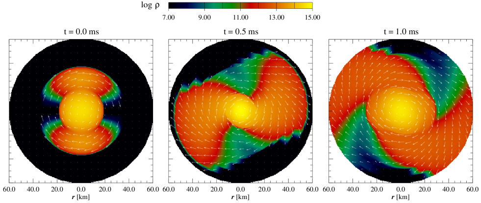
Figure 14: Evolution of a strongly distorted nonaxisymmetric rotating neutron star model. The color coded distribution of $\log\rho$ on the equatorial plane shows how the initial perturbation (left panel) is partly accreted by the neutron star, and partly stretched into spiral arms (center panel). After about one rotation period of the neutron star, the trailing spiral arms have grown considerably in size (right panel). The rotation velocity $v_{\varphi}$ is indicated by white arrows. Note that the atmosphere (color coded in black) has a density of much less than $10^{7}{\rm\ g\ cm}^{-3}$, and that only the innermost 60 km of the computational domain are shown.

On top of the equilibrium neutron star model we add a strongly nonaxisymmetric (i.e. $\varphi$-dependent) perturbation of the rest-mass density

$$\rho=\rho_{\rm ini}+a\,\rho_{\rm c}\,\sin^{2}\!\left[\pi\left(\frac{r}{2r_{\rm s}}\right)^{2}\right]\sin^{10}\varphi\quad\mbox{for }r\leq 2r_{\rm s},$$ (47)

with an amplitude $a=0.1$, which yields an $l=m=2$ bar-like structure. The rotation velocity of the uniformly rotating unperturbed neutron star is extrapolated into the areas filled with matter by the perturbation. The initial configuration with the perturbation added is shown in the left panel of Fig. 14.

We have chosen this particular (albeit unphysically strong) perturbation and velocity field in order to prevent both, an immediate accretion of the added matter bars on to the neutron star or an ejection. This allows us to follow the rotation of the neutron star for a time comparable to its rotation period (which is about 1 ms for the unperturbed neutron star). The density and rotation velocity plots in Fig. 14 after $t=0.5{\rm\ ms}$ (center panel) and $t=1.0{\rm\ ms}$ (right panel) prove this property of the chosen perturbation. These plots also demonstrate that the corotating bar structures slowly disappear. The innermost parts are being gradually accreted by the neutron star, which leads to a significant initial rise in the central density, as shown in Fig. 15. At later times the more massive neutron star oscillates with a period of $t_{\rm osc}\sim 1.0{\rm\ ms}$ around a new quasi-equilibrium state, which possesses a central density of more than 50% above the initial equilibrium central density. Despite this strong interaction of the bar perturbation with the neutron star, the rotation profile inside the neutron star remains uniform throughout the evolution, although the rotation velocity nearly doubles during the oscillation maxima. This behavior is most likely due to the particular choice of a uniform rotation profile for the initial bar perturbation.

For the outer parts of the initial bar, the increasing distance from the neutron star and the sufficiently high specific angular momentum prevents their accretion onto the neutron star. Thus the matter in this region of the bar drifts to larger radii during the evolution. As on the dynamical timescales considered of one rotation period there is no efficient transport mechanism of local angular momentum by viscous effects (which act on much longer timescales), the evolution leads to the development of spiral arms which are clearly visible in the middle and right panels of Fig. 14. The outer parts of these arms are centrifugally expelled from the finite difference grid, crossing the outer boundary at $t\sim 0.84{\rm\ ms}$. By the end of the simulation, at $t=4{\rm\ ms}$, there is neither significant backscattering of matter from the outermost boundary of the radial grid, nor there are numerical artifacts visible at the leading or trailing edges of the spiral arms. This proves that our numerical treatment of the radial boundary conditions and of the artificial low density atmosphere surrounding the star have the desired behavior.

Figure 15: Time evolution of the central density $\rho_{\rm c}$ for distorted nonaxisymmetric rotating neutron star models. If the distortion is strong ($a=0.1$, solid line), matter accretion from the rotating bars results in a steep initial increase of $\rho_{\rm c}$, which slowly settles down to a new equilibrium state (indicated by the horizontal dotted line). For a small perturbation ($a=0.01$, dashed line), the evolution of $\rho_{\rm c}$ follows very closely that of an unperturbed model (dashed-dotted line).

Fig. 15 shows that already after an evolution time of $\sim 1{\rm\ ms}$, the evolution of the spiral arms has no further significant impact in the dynamics of the neutron star, as then the slowly decaying oscillation around the final equilibrium state exhibits a rather regular ring-down pattern. Plotted in this figure is also the time evolution of the central density for a model with an amplitude $a=0.01$ of the initial perturbation given by Eq. (47) (dashed line). In addition, the dashed-dotted line shows the corresponding time evolution of $\rho_{\rm c}$ for an unperturbed model (the small amplitude oscillations are in this case triggered by the truncation errors of the numerical schemes and by the use of the CFC approximation in the evolution code). The similarity in the behavior of $\rho_{\rm c}$ in these cases demonstrates that for perturbations with an amplitude $a\lesssim 0.01$, the dynamics of the central neutron star is virtually unaffected by the initial bar and by the spiral arms forming at later times. However, we observe that also for small values of $a$ spiral arms develop which are stable over many rotation periods.

Figure 16: Gravitational wave signal for distorted nonaxisymmetric rotating neutron star model. If the distortion is strong ($a=0.1$, solid lines), the nonzero gravitational wave amplitudes $A_{+}^{\rm e}$ (upper panel), $A_{+}^{\rm p}$ (center panel), and $A_{\times}^{\rm p}$ (lower panel) reach peak values of up to $\sim 15,000{\rm\ cm}$. The amplitudes reduce significantly for $a=0.01$ (dashed lines). If an axisymmetric perturbation with $a=0.1$ is applied (dashed-dotted line), only the $A_{+}^{\rm e}$ gravitational wave mode is present.

Apparently, strong nonaxisymmetric perturbations of the form (47) give rise to significant gravitational wave emission. The waveforms of the nonzero gravitational wave amplitudes $A_{+}^{\rm e}$, $A_{+}^{\rm p}$, and $A_{\times}^{\rm p}$ (as shown in the upper, center, and lower panel of Fig. 16, respectively) exhibit peak values of up to $\sim 15\times 10^{3}{\rm\ cm}$ for the model with a perturbation amplitude $a=0.1$ (solid lines). In Fig. 16 we also present the waveforms for the model with a bar perturbation of amplitude $a=0.01$ (dashed lines). Their amplitudes are roughly a factor 10 smaller than those of the corresponding waveforms of the model with $a=0.1$. Thus we can infer that the gravitational radiation amplitude approximately scales with $a$.

We emphasize that owing to the particular form of the perturbation (47), the $\times$-mode of the gravitational radiation is zero at the equator, $A_{\times}^{\rm e}=0$. We also note that if instead of the nonaxisymmetric perturbation in Eq. (47) we use an axisymmetric one,

$$\rho=\rho_{\rm ini}+a\,\rho_{\rm c\,ini}\,\sin^{2}\left[\pi\left(\frac{r}{2r_{\rm s}}\right)^{2}\right]\quad\mbox{for }r\leq 2r_{\rm s},$$ (48)

then the $\times$-mode of gravitational radiation vanishes completely, and only the $+$-mode is present (dashed-dotted line in the upper panel of Fig. 16). Additionally, in axisymmetry the $+$-mode on the pole is always zero, $A_{+}^{\rm p}=0$.

We point out that the waveform pattern for the model with the $a=0.1$ bar perturbation in Fig. 16 does not solely reflect the oscillation and ring-down structure of the central neutron star, as visible in the time evolution of $\rho_{c}$ in Fig. 15. For instance the $+$-mode at the equator (upper panel) decays on a much longer time scale than the corresponding ring-down time of $\rho_{c}$. On the other hand, the waveforms for the two polarizations of the radiation at the pole exhibit their peaks during the first oscillation of $\rho_{c}$ and then decay rapidly (center and lower panel). However, after an evolution time of $\sim 2{\rm\ ms}$ their amplitudes increase again. From this behavior we deduce that initially the waveform signal is dominated by the gravitational wave emission from the oscillating neutron star. As this contribution decays during the ring-down, the wave emission from spiral arms becomes increasingly important. As they expand into the atmosphere the radial weight arm in the quadrupole formula compensates for the relatively low density of the spiral arms, and the radiation emitted in this region becomes visible in the signal. We cannot clearly attribute the late-time increase in the waveform amplitude to the onset of a bar mode instability, because the rotation parameter $\beta$ of our model clearly falls short of the approximate threshold for dynamical growth of bar modes: $\beta\sim 0.14\ll\beta_{\rm d}$. We plan to investigate this issue more thoroughly in the future.

The maximum amplitude $A\sim 15\times 10^{3}{\rm\ cm}$ of the wave signal for $a=0.1$ corresponds to a dimensionless gravitational wave amplitude $h\sim 5\times 10^{-19}$ at a distance of $r=10{\rm\ kpc}$ to the source. Thus, in this case of a strongly nonaxisymmetric artificial perturbation, the typical wave amplitudes have a value of roughly one order of magnitude above the ones of waveforms obtained from the simplified models of rotational supernova core collapse in axisymmetry by Dimmelmeier et al. dimmelmeier_02_b . For the waveforms plotted in Fig. 16 we utilize the stress formula (38) with $\rho^{*}$ as density. The use of this formula efficiently reduces the numerical noise in the signal as compared with the first moment of momentum density formula and particularly with the standard quadrupole formula.

We consider the grid resolution used in this test simulation to be the minimal one required for obtaining reasonably converged results. By repeating the same model with different grid resolutions we are able to estimate that the waveform amplitudes are correctly computed within $\sim 30\%$ accuracy.

V Conclusions

In this paper we have presented a new three-dimensional general relativistic hydrodynamics code which is primarily intended for applications of stellar core collapse to a neutron star or a black hole, as well as for studies of rapidly rotating relativistic stars which may oscillate in their quasi-normal modes of pulsation, emitting gravitational radiation, or which may be subject to nonaxisymmetric instabilities. The main novelty of this code compared to other existing numerical relativistic codes is that it combines very accurate state-of-the-art numerical methods specifically tailored to solve the general relativistic hydrodynamics equations on the one hand, and the gravitational field equations on the other hand. More precisely, the hydrodynamic equations, formulated in conservation form, are solved using high-resolution shock-capturing schemes based upon approximate Riemann solvers and third-order cell-reconstruction interpolation procedures, while the elliptic metric equations are solved using an iterative nonlinear solver based on spectral methods. Furthermore, the present code also departs noticeably from other three-dimensional codes in the coordinate system used in the formulation of the equations and in the discretization. In our approach both the metric and the hydrodynamics equations are formulated and solved numerically using spherical polar coordinates. In the present investigation we have adopted the so-called conformal flatness approximation of the Einstein equations, which reduces them to a set of five elliptic nonlinear equations, particularly suited for the use of spectral methods. Recently, constrained formulations of the full Einstein equations in which elliptic equations have a preeminence over hyperbolic equations have been reported, and appear to be amenable to the current code.

The main purpose of the paper has been to assess the code by demonstrating that the combination of the finite difference grid and the spectral grid, on which the hydrodynamics and metric equations are respectively solved, can be successfully accomplished. This approach, which we call Mariage des Maillages (French for grid wedding), results in high accuracy of the metric solver and, in practice, has allowed for fully three-dimensional applications using computationally affordable resources, along with ensuring long term numerical stability of the evolution. To facilitate the Mariage des Maillages, i.e. the combination of the finite difference grid for the hydrodynamic solver and the spectral grid for the metric solver, a sophisticated interpolation and grid communication scheme has been used. In addition, we have compared our novel approach to two other, finite difference based, methods to solve the metric equations, which we already employed in earlier axisymmetric investigations dimmelmeier_02_a ; dimmelmeier_02_b .

We have presented a variety of tests in two and three dimensions, involving neutron star spacetimes and stellar core collapse. Axisymmetric simulations have also been performed to compare core collapse to neutron stars using the CFC approximation and full general relativity, for which only very recently results have become available shibata_04_a . This comparison has shown the suitability of the conformally flat approximation for such mildly relativistic scenarios. Furthermore, the code has succeeded in simulating the highly perturbed nonaxisymmetric configuration of a uniformly rotating neutron star for several dynamical times. This simulation has also been used to assess the 3D gravitational waveform extraction capabilities of the code. In summary the numerical experiments reported in the paper demonstrate the ability of the code to handle spacetimes with and without symmetries in strong gravity. In future work we plan to apply this code to simulations of stellar core collapse to neutron stars or black holes in three dimensions, and particularly to studies of the nonlinear development of bar mode instabilities in rapidly rotating neutron stars.

Appendix A Differences to previous 2D CFC simulations

A.1 Compact form of the Euler equation sources

In the axisymmetric CFC code presented in dimmelmeier_02_a ; dimmelmeier_02_b the source terms $Q_{j}$ for the hydrodynamic momentum equations (Euler equations) were evaluated on the finite difference grid using a formulation containing time derivatives and explicit Christoffel symbols (see Equation (4)):

$$Q_{j}=T^{\mu\nu}\left(\frac{\partial g_{\nu j}}{\partial x^{\mu}}-{\it\Gamma}^{\lambda}_{\mu\nu}g_{\lambda j}\right).$$ (49)

Using the relation between the Christoffel symbols and the derivatives of the spacetime metric,

$${\it\Gamma}^{\lambda}_{\mu\nu}=\frac{1}{2}g^{\lambda\delta}\left(\frac{\partial g_{\delta\nu}}{\partial x^{\mu}}+\frac{\partial g_{\delta\mu}}{\partial x^{\nu}}-\frac{\partial g_{\mu\nu}}{\partial x^{\delta}}\right),$$ (50)

the sources $Q_{j}$ can be written in a more compact form as

$$Q_{j}=\frac{1}{2}T^{\mu\nu}\frac{\partial g_{\mu\nu}}{\partial x^{j}}.$$ (51)

In this formulation, only spatial derivatives of the metric are needed, and the numerical evaluation of $Q_{j}$ involves significantly fewer terms, making a numerical implementation both faster and more accurate. For these reasons, we have preferred the use of Equation (51) to Equation (49) in the code presented in this paper.

A.2 Exact numerical conservation of the hydrodynamic equations

As emphasized in Section 5.4 in dimmelmeier_02_a , the conserved hydrodynamic quantity in the system of conservation equations (3) is not simply the state vector $U$ but rather $\sqrt{\gamma}\mbox{\boldmath$U$}$ with $\sqrt{\gamma}=\phi^{6}r^{2}\sin\theta$. Therefore, if only the state vector $U$ is evolved, this gives rise to an additional source term $\hat{Q}$ which contains time derivatives of the conformal factor $\phi$. These generally time-dependent source terms result in a variation of the volume-integrated state vector with time, and thus in a violation of exact numerical rest mass and angular momentum conservation of several percent, even though the “physical” sources vanish, $\mbox{\boldmath$Q$}=0$ (see Figs. 9 and 10 in Ref. dimmelmeier_02_a ).

It is not possible to evolve $\sqrt{\gamma}\mbox{\boldmath$U$}$ in a straightforward way and then consistently solve the elliptic metric equations (11) on the new time slice. This is due to the fact that the sources for these equations contain the pressure $P$, which can only be extracted from $U$ but not from $\sqrt{\gamma}\mbox{\boldmath$U$}$. However, one can make use of the time evolution equation for the conformal factor, Eq. (9), to obtain an auxiliary value for $\phi$ and thus for $\sqrt{\gamma}$ on the new time slice. With this the state vector $U$ can be consistently calculated from $\sqrt{\gamma}\mbox{\boldmath$U$}$ after the time evolution step to the new time slice, which in turn is used in the sources of the metric equations (11). These are subsequently solved on the new time slice. With the help of this reformulation of the hydrodynamic time evolution problem in the current code (in combination with the compact time-independent form for the sources in the Euler equations, Eq. (51)), we are able to achieve exact numerical conservation of the total rest mass and angular momentum up to machine roundoff errors, provided that there is no artificial atmosphere and no mass flow across the outer radial grid boundary.

A.3 Shift vector boundary conditions

The results for the evolution of the central density $\rho_{\rm c}$ and the waveform for the core collapse model SCC (A3B2G4 in dimmelmeier_02_b ) presented in this paper slightly differ from those reported in the previous paper by Dimmelmeier et al. dimmelmeier_02_b . This is partly due to the improvements related to evaluating the Euler equation source terms in compact form and using exact numerical conservation in the new code, as discussed above. However, the main reason for the small discrepancy is that in the simulations in dimmelmeier_02_b a symmetric boundary condition for the shift vector component $\beta^{2}$ across the equatorial plane was chosen. This leads to a nonzero value for $\beta^{2}$ at $\theta=\pi/2$ close to and after core bounce, i.e. when meridional motions set in. As a consequence of this, the deviation is stronger for models where rotation plays a significant role in the collapse dynamics.

The physically accurate antisymmetric equatorial boundary condition for $\beta^{2}$ which is used in the present code, systematically yields lower post-bounce values for $\rho_{\rm c}$ in regular collapse type models compared to the simulations presented in dimmelmeier_02_b , with a difference of 11% on average. For models which show multiple bounce behavior, we obtain a lower $\rho_{\rm c}$ also at core bounce.

Accordingly, the waveform amplitudes and frequencies of the gravitational radiation are altered by a small amount (-11% for $|A^{\rm E2}_{20}|_{\rm max}$ and -18% for $\nu$). Despite of these small quantitative changes, the qualitative statements related to the influence of general relativistic effects in rotational core collapse made by Dimmelmeier et al. dimmelmeier_02_b remain unaffected, even when the antisymmetric boundary condition is used. We particularly emphasize that the change in the boundary condition for $\beta^{2}$ plays no role when comparing our results with the fully general relativistic simulations by Shibata and Sekiguchi shibata_04_a discussed in Section IV.2.4.

We note that for all core collapse models presented in the parameter study by Dimmelmeier et al. dimmelmeier_02_b , results obtained with the new boundary condition for $\beta^{2}$ can be found in the revised waveform catalogue garching_results .

References

- (1) R. Buras, M. Rampp, H.-T. Janka, and K. Kifonidis, Phys. Rev. Lett. 90, 241101 (2003).
- (2) E. Müller, in O. Steiner and A. Gautschy, eds., Computational methods for astrophysical fluid flow, Saas-Fee Advanced Course 27, 343 (Springer, Berlin, 1998).
-
(3)
K. New,
Living Rev. Relativ. 6, 2 (2003);
http://www.livingreviews.org/lrr-2003-2/. - (4) E. Müller, Astron. Astrophys. 114, 53 (1982).
- (5) L. S. Finn and C. R. Evans, Astrophys. J. 351, 588 (1990).
- (6) R. Mönchmeyer, G. Schäfer, E. Müller, and R. E. Kates, Astron. Astrophys. 246, 417 (1991).
- (7) S. Yamada and K. Sato, Astrophys. J. 450, 245 (1995).
- (8) T. Zwerger and E. Müller, Astron. Astrophys. 320, 209 (1997).
- (9) M. Rampp, E. Müller, and M. Ruffert, Astron. Astrophys. 332, 969 (1998).
- (10) H. Dimmelmeier, J. A. Font, and E. Müller, Astrophys. J. Lett. 560, L163 (2001).
- (11) H. Dimmelmeier, J. A. Font, and E. Müller, Astron. Astrophys. 388, 917 (2002).
- (12) H. Dimmelmeier, J. A. Font, and E. Müller, Astron. Astrophys. 393, 523 (2002).
- (13) C. L. Fryer, D. E. Holz, and S. A. Hughes, Astrophys. J. 565, 430 (2002).
- (14) C. L. Fryer, D. E. Holz, S. A. Hughes, and M. S. Warren, http://www.arxiv.org/abs/astro-ph/0211609/.
- (15) J. N. Imamaura, B. K. Pickett, and R. H. Durisen, Astrophys. J. 587, 341 (2003).
- (16) K. Kotake, S. Yamada, and K. Sato, Phys. Rev. D, 68, 044023 (2003).
- (17) M. Shibata and Y. I. Sekiguchi, Phys. Rev. D (2004, in press).
- (18) C. D. Ott, A. Burrows, E. Livne, and R. Walder, Astrophys. J. 602, 834 (2004).
- (19) E. Müller, H.-T. Janka, Astron. Astrophys. 317, 140 (1997).
- (20) E. Müller, M. Rampp, R. Buras, H.-T. Janka, and D. H. Shoemaker, Astrophys. J. 603, 221 (2004).
- (21) A. Burrows and J. Hayes, Phys. Rev. Lett., 76, 352 (1996).
- (22) L. Lehner, Class. Quantum Grav. 18, R25 (2001).
- (23) L. Lindblom and M. A. Scheel, Phys. Rev. D 67, 124005 (2003).
- (24) J. A. Isenberg, “Waveless approximation theories of gravities”, University of Maryland Preprint (1978, unpublished).
- (25) J. R. Wilson, G. J. Mathews, and P. Marronetti, Phys. Rev. D 54, 1317 (1996).
- (26) http://www.mpa-garching.mpg.de/rel_hydro/.
- (27) T. Pradier, N. Arnaud, M.-A. Bizouard, F. Cavalier, M. Davier, and P. Hello, Phys. Rev. D 63, 042002 (2001).
- (28) M. Shibata and T. Nakamura, Phys. Rev. D 52, 5428 (1995).
- (29) T. W. Baumgarte and S. L. Shapiro, Phys. Rev. D 59, 024007 (1999).
- (30) T. Nakamura, K. Oohara, and Y. Kojima, Prog. Theor. Phys. Suppl. 90, 1 (1987).
- (31) F. Siebel, J. A. Font, E. Müller, and P. Papadopoulos, Phys. Rev. D 67, 124018 (2003).
- (32) D. Gottlieb and S. A. Orszag, Numerical analysis of spectral methods: theory and applications (Society of Industrial and Applied Mathematics, Philadelphia, 1977).
- (33) C. Canuto, M. Y. Hussaini, A. Quarteroni, and T. A. Zang, Spectral methods in fluid dynamics (Springer, Berlin, 1988).
- (34) S. Bonazzola and J. A. Marck, J. Comput. Phys. 87, 201 (1990).
- (35) http://www.luth.obspm.fr/Groupe1.html.
- (36) S. Bonazzola, E. Gourgoulhon, and J.-A. Marck, J. Comput. App. Math. 109, 433 (1999).
- (37) L. Villain and S. Bonazzola, Phys. Rev. D 66, 123001 (2002).
- (38) P. Grandclément, E. Gourgoulhon, and S. Bonazzola, Phys. Rev. D 65, 044021 (2002).
- (39) S. Bonazzola, E. Gourgoulhon, P. Grandclément, and J. Novak, Phys. Rev. D, (2003, submitted); gr-qc/0307082.
- (40) http://www.lorene.obspm.fr.
- (41) J. Frauendiener, J. Comput. Appl. Math. 109 475 (1999).
- (42) H. P. Pfeiffer, L. E. Kidder, M. A. Scheel, and S. A. Teukolsky, Comput. Phys. Commun. 152, 253 (2003).
- (43) E. F. Toro, Riemann solvers and numerical methods for fluid dynamics – a practical introduction (Springer, Berlin, 1997).
-
(44)
J. A. Font,
Living Rev. Relativ. 6, 4 (2003);
http://www.livingreviews.org/lrr-2003-4/. - (45) J. M. Martí and E. Müller, Living Rev. Relativ. 6, 7 (2003); http://www.livingreviews.org/lrr-2003-7/.
- (46) P. Cerdá-Durán, G. Faye, H. Dimmelmeier, J. A. Font, J. M. Ibáñez, E. Müller, and G. Schäfer, (2004, in preparation).
- (47) G. Schäfer and A. Gopakumar, Phys. Rev. D 69, 021501 (2004).
- (48) J. Novak and J. M. Ibáñez, Astrophys. J. 533, 392 (2000).
- (49) J. A. Font, M. Miller, W.-M. Suen, and M. Tobias, Phys. Rev. D 61, 044011 (2000).
- (50) J. A. Font, T. Goodale, S. Iyer, M. Miller, L. Rezzolla, E. Seidel, N. Stergioulas, W.-M. Suen, and M. Tobias, Phys. Rev. D 65, 084024 (2002).
- (51) M. Shibata, Phys. Rev. D 60, 104052 (1999).
- (52) M. D. Duez, T. W. Baumgarte, S. L. Shapiro, M. Shibata, and K. Uryu, Phys. Rev. D 65, 024016 (2002).
- (53) L. Baiotti, I. Hawke, P. J. Montero, F. Löffler, L. Rezzolla, N. Stergioulas, J. A. Font, and E. Seidel, Phys. Rev. D (2004, submitted).
- (54) http://www.aei-potsdam.mpg.de/~hawke/Whisky.html.
- (55) F. Banyuls, J. A. Font, J. M. Ibáñez, J. M. Martí, and J. A. Miralles, Astrophys. J. 476, 221 (1997).
- (56) H.-T. Janka, T. Zwerger, and R. Mönchmeyer, Astron. Astrophys. 268, 360 (1993).
- (57) R. Arnowitt, S. Deser, and C. W. Misner, in L. Witten, ed., Gravitation: An introduction to current research (Wiley, New York, 1962).
-
(58)
O. Reula,
Living Rev. Relativ. 1, 3 (1998);
http://www.livingreviews.org/lrr-1998-3/. - (59) T. Damour, E. Gourgoulhon and P. Grandclément, Phys. Rev. D 66, 024007 (2002).
- (60) C. R. Evans, in Dynamical Spacetimes and Numerical Relativity, ed. J. Centrella, 3, (Cambridge University Press, 1986).
- (61) R. F. Stark, in Frontiers in Numerical Relativity, eds. C. R. Evans, L. S. Finn, and D. W. Hobill, 281, (Cambridge University Press, 1989).
- (62) J. P. Boyd, Chebyshev and Fourier Spectral Methods, second edition (Dover, New York, 2001).
- (63) R. Donat, J. A. Font, J. M. Ibáñez, and A. Marquina, J. Comput. Phys. 146, 58 (1998).
- (64) M. Shibata, Phys. Rev. D 67, 024033 (2003).
- (65) D. Potter, Computational physics (Wiley, Chichester, U. K., 1973).
- (66) P. Grandclément, S. Bonazzola, E. Gourgoulhon, and J. A. Marck, J. Comput. Phys. 170, 231 (2001).
- (67) L. S. Finn, in C. R. Evans, S. L. Finn, and D. W. Hobbill, eds., Frontiers in numerical relativity, 126 (Cambridge University Press, Cambridge, 1989).
- (68) L. Blanchet, T. Damour, and G. Schäfer, Mon. Not. R. Astron. Soc. 242, 289 (1990).
- (69) M. Shibata and Y. I. Sekiguchi, Phys. Rev. D 68, 104020 (2003).
- (70) H. Komatsu, Y. Eriguchi, and I. Hachisu, Mon. Not. R. Astron. Soc. 237, 335 (1989).
- (71) J. A. Font, N. Stergioulas, and K. D. Kokkotas, Mon. Not. R. Astron. Soc. 313, 678 (2000).
- (72) M. Alcubierre, S. Brandt, B. Brügmann, D. Holz, E. Seidel, R. Takahashi, and J. Thornburg, Int. J. Mod. Phys. D 10, 273 (2001).
-
(73)
K. D. Kokkotas and B. G. Schmidt,
Living Rev. Relativ. 2, 2 (1999);
http://www.livingreviews.org/lrr-1999-2/. - (74) J. A. Font, H. Dimmelmeier, A. Gupta, and N. Stergioulas, Mon. Not. R. Astron. Soc. 325, 1463 (2001).
- (75) N. Stergioulas, T. A. Apostolatos, and J. A. Font, Mon. Not. R. Astron. Soc. (2004, in press).
- (76) H. Dimmelmeier, N. Stergioulas, and J. A. Font (2004, in preparation).