Angular diameters, fluxes and extinction of compact planetary nebulae: further evidence for steeper extinction towards the Bulge

Abstract

We present values for angular diameter, flux and extinction for 70 Galactic planetary nebulae observed using narrow band filters. Angular diameters are derived using constant emissivity shell and photoionization line emission models. The mean of the results from these two models are presented as our best estimate. Contour plots of 36 fully resolved objects are included and the low intensity contours often reveal an elliptical structure that is not always apparent from FWHM measurements. Flux densities are determined, and for both H$\alpha$ and [O iii] there is little evidence of any systematic differences between observed and catalogued values. Observed H$\alpha$ extinction values are determined using observed H$\alpha$ and catalogued radio fluxes. H$\alpha$ extinction values are also derived from catalogued H$\alpha$ and H$\beta$ flux values by means of an $R_{\mathrm{V}}$ dependent extinction law. $R_{\mathrm{V}}$ is then calculated in terms of observed extinction values and catalogued H$\alpha$ and H$\beta$ flux values. Comparing observed and catalogue extinction values for a subset of Bulge objects, observed values tend to be lower than catalogue values calculated with $R_{\mathrm{V}}=3.1$. For the same subset we calculate $\langle R_{\mathrm{V}}\rangle=2.0$, confirming that toward the Bulge interstellar extinction is steeper than $R_{\mathrm{V}}=3.1$. For the inner Galaxy a relation with the higher supernova rate is suggested, and that the low-density warm ionized medium is the site of the anomalous extinction. Low values of extinction are also derived using dust models with a turnover radius of 0.08 microns.

1 Introduction

The angular diameter and flux of a planetary nebula (PNe) are much needed parameters when modelling the optical spectrum and evolution of the nebula and its central star. From these parameters the density and mass of the PNe can be calculated, as well as the extinction along the line of sight. PNe also provide an independent tracer of stellar populations and extinction in regions where visual tracers, such as hot luminous stars, are lacking.

At the distance of the Bulge of $R=8$ kpc (Reid, 1993) many PNe are only a few arc seconds across. Therefore determination of angular diameters, by deconvolving FWHM measurements, need to use methods that take into account ionisation structure and the particular emission line observed. Bedding & Zijlstra (1994, hereafter BZ) and van Hoof (2000, hereafter VH) provide two suitable methods of deconvolution.

Spectroscopic flux measurements can lead to a possible underestimation if the slit is not properly aligned with the source. Therefore accurate determination of fluxes can be achieved using calibrated narrow-band filters, provided that correction for the underlying continuum and any unwanted lines is applied. Extinction can then be calculated from observed H$\alpha$ and catalogue radio flux ratios, and compared with values calculated from catalogue H$\alpha$/H$\beta$ flux ratios. A method for determining $R_{\mathrm{V}}$, the ratio of total to selective extinction, can also be derived.

Correction for interstellar extinction is necessary for determining emission line ratios, absolute fluxes, and some distance calculations. Usually, a single Galactic extinction law is used for dereddening. However, the emission mechanism of ionized media is well understood, and PNe are intrinsically very bright. This allows one to use PNe to determine extinction constants for Galactic dust distribution studies, for line of sights where few other good tracers are available.

In order to improve the accuracy of available PNe data, we have obtained narrow-band H$\alpha$ and [O iii] CCD images of a sample of Galactic PNe and calculated values for angular diameter, flux and extinction.

Table 1: Filter characteristics (Å).

Filter	ESO#	Peak	Centre	FWHM	$\int T\mathrm{d}\lambda$
H$\alpha$ on-band*	654	6546	6549	32	11
H$\alpha$ off-band	598	6675	6673	65	37
$[$O iii$]$ on-band*	589	5016	5014	55	36
$[$O iii$]$ off-band	591	5100	5110	60	43

*Calculated from observed spectra.

2 Observations and data processing

We observed 70 Galactic PNe during the two nights of 2002 June 24 & 25, using the ESO 3.5-m New Technology Telescope (NTT) in Chile. We used the EMMI camera (ESO Multi-Mode Instrument), which at the time had a 2046 $\times$ 2046 pixel Tektronix CCD with an image scale of 0$\aas@@fstack{\prime\prime}$27/pixel. For each object a pair of exposures were taken using on- and off-band H$\alpha$ filters. 16 of the objects were also observed with on- and off-band [O iii] filters. The FWHM of the on-band filters are adapted to the high velocity range of the observed PNe (200 to 300 km s^-1 in the Galactic bulge, corresponding to $\sim$ 5Å). The characteristics of the filters, in Å, are listed in Table 1 and plotted in Fig. 1. It should be noted that, to avoid contamination by the [N ii] 6584Å line, the H$\alpha$ on-band filter is centred on 6549Å and not 6563Å.

In Fig. 1 the dashed curves are the filter response values provided by ESO, and the solid curves are response values calculated from calibration spectra taken at the NTT (H$\alpha$ in 2004 February using Grism #3 at a resolution of 1.5Å, interpolated to 0.1Å; [O iii] in 2003 June using Grism #3 at a resolution of 3Å, interpolated to 1Å). The solid vertical lines denote La Silla-air wavelengths and the dashed vertical lines the spread of observed wavelengths due to Doppler shifting. Assuming the same equivalent widths, the H$\alpha$ on-band filter #654 has blue-shifted by $\sim 5$Å and the [O iii] on-band filter #589 has red-shifted by $\sim 7$Å. It can be seen that for [O iii] this shift makes little difference to the calculation of actual flux values. However, for H$\alpha$ the shift is significant, as actual observed wavelengths are in the steep redward side of the curve (especially for positive radial velocities relative to the telescope).

Because the filters in the red arm of EMMI are used in the parallel beam, there is a large change in central wavelength with position on the detector. The solid curve is given for the optical centre of the field. Because objects were not always positioned at the optical centre of the CCD array (up to $\pm 20$ pixels on the first night and up to $\pm 50$ pixels on the second), wavelength corrections were calculated to take into account the filter angle of 7.5°relative to the CCD array. This only affected offsets in the $y$-axis, with a 20 pixel offset generating a wavelength shift of 0.6Å. For these reasons, in particular, we chose to calculate precise Doppler wavelength shifts when determining actual observed flux values. We have not been able to determine the reason for the shift in filter transmission curves, so would therefore recommend always taking calibration spectra from the optical centre of the field in order to check filter response data.

To reduce the CCD readout time and hence improve the observing duty cycle, only the central 400 $\times$ 400 pixels (108″ $\times$ 108″) of the detector were read out. Calibration of the CCD images followed standard procedures: subtraction of a constant value to represent the bias, and removal of the background continuum, achieved by subtracting the off-band image, scaled by the integrated transmission ratio of the two filters ($\int T_{\mathrm{on}}\mathrm{d}\lambda\ /\int T_{\mathrm{off}}\mathrm{d}\lambda$), from the on-band image. The ratios were 0.31 for the H$\alpha$ filter and 0.84 for the [O iii] filter. Where necessary and prior to this subtraction, pairs of images were brought into alignment by integer pixel shifts of the off-band image in the $x$ and/or $y$ direction. For the first night’s observations this involved shifts of only one or two pixels. However, due to taking spectra between on- and off-band exposures, the second night’s observations required shifts of between 20 and 30 pixels. One off-band image (356.1$+$02.7 Th3-13) had to be rotated as well, to bring it into alignment. This procedure removed the background field stars, except for objects with spectral lines within the filter band. Correction with dome flats was not considered necessary due to the sources being very small and pixel to pixel variations in the centre of the CCD contributing a possible error in flux values of only 1 per cent.

       

Figure 1: Transmission curves for on-band H$\alpha$ and [O iii] filters. Dashed curves are filter response values provided by ESO and solid curves are those based on observed calibration spectra. Solid vertical lines indicate La Silla-air wavelengths, with dashed vertical lines indicating the spread of observed wavelengths due to Doppler shifting.

All exposures were for 30 seconds with the autoguider deactivated, as the NTT can track without guiding for several minutes. The resulting images show no sign of elongation of the field stars. Ten second exposures of two tertiary standard stars were also taken for flux calibration. Seeing conditions varied between one and two arc seconds. Subsequent image analysis was done using the ESO Munich Image Data Analysis System (midas).

Bulge PNe were concentrated on, but non-Bulge objects were also observed to make best use of telescope time. Using a Galactic Bulge criteria for the galactic coordinates (PN G) of $|l|<15\degr$ and $|b|<15\degr$ gives 56 Bulge PNe and 14 non-Bulge PNe. However, adopting the criteria of Bensby & Lundström (2001): $|l|<10\degr$ and $|b|<10\degr$; $0\aas@@fstack{\prime\prime}9<\theta<20\arcsec$; 4.2 mJy $<S_{5\,\mathrm{GHz}}<$ 45 mJy, gives 39 Bulge PNe and 31 non-Bulge PNe. The non-Bulge PNe include two Sagittarius dwarf galaxy objects (Dudziak et al., 2000).

3 Diameter determinations

3.1 Method

The images presented here are broadened by the seeing. This must be taken into account when deriving angular diameters and we now describe the methods used to deconvolve the point spread function (beam size).

Using the method of BZ, the point spread function (PSF) was approximated with a Gaussian FWHM of $\theta_{\mathrm{PSF}}$, by fitting Gaussian profiles to four distinct field stars in each of the on-band images, taking the mean value and expressing the error as the standard deviation of the four readings. The results are listed in column four of Table 4, with an overall mean value for $\theta_{\mathrm{PSF}}$ of 1$\aas@@fstack{\prime\prime}$55. The FWHM of the nebulae $\theta_{\mathrm{FWHM}}$, was measured by fitting two dimensional Gaussian profiles to the corrected on-band images. As BZ point out, if the objects were Gaussian, deconvolution would be trivial, and the true FWHM of the nebulae would simply be

$$\theta_{\mathrm{gauss}}=\sqrt{(\theta_{\mathrm{FWHM}})^{2}-(\theta_{\mathrm{PSF}})^{2}}.$$ (1)

Although $\theta_{\mathrm{gauss}}$ is not a realistic model for PNe, a correction factor $\gamma$, can be applied in order to determine the true diameter, $\theta_{\mathrm{true}}=\gamma\theta_{\mathrm{gauss}}$. Various methods of calculating this factor have been investigated by VH and the conversion factor $\gamma$ is found to be a function of $\beta$, the resolution of the observation, i.e. the ratio of the Gaussian diameter and the point spread function, $\beta=\theta_{\mathrm{gauss}}/\theta_{\mathrm{PSF}}$. According to VH, $\gamma(\beta)$ can be approximated extremely well by the following analytic function (VH method A):

$$\gamma(\beta)=\frac{a_{1}}{1+a_{2}\beta^{2}}+a_{3},$$ (2)

which will be used throughout this paper (appropriate parameters for equation 2 are given in Table 2).

Table 2: The parameters (van Hoof, 2000, tables 1 & 2) for calculating conversion factors using equation 2.

Model	a1	a2	a3
Constant emissivity shell 0.8	0.3893	0.7940	1.2281
H$\alpha$ emission line shell	0.3605	0.7822	1.4937
$[$O iii$]$ emission line shell	0.4083	0.7892	1.3176

VH finds that the method used by BZ for the calculation of $\gamma$ for disk, sphere and shell geometries is essentially identical to his own method B, with results that are also in good agreement with his method A (see VH fig. 3), apart from a slight overestimation of $\gamma$ for larger values of $\beta$. In the case of a constant emissivity shell, VH fig. 2 shows that the shape of the curve for the conversion factor $\gamma$ does not change very much as a function of $r_{\mathrm{i}}/r_{\mathrm{s}}$, but that the height of the curve does. Therefore, the correct value for $\gamma$ depends critically on the assumed value for the inner radius, $r_{\mathrm{i}}$, with differences of up to 40 per cent, depending on the choice $r_{\mathrm{i}}$. VH also examines what he considers to be more realistic geometries based on a photoionization model of PNe. This model takes into account emissivity and absorption of specific lines as a function of distance to the star. As VH point out, the surface brightness profile is very sensitive to optical depth effects and thus different emission lines will yield different diameters. Measured diameters will also be different, depending on which line is used, because of ionisation stratification effects. VH also present an alternative algorithm for determination of the intrinsic FWHM of a source, using the observed surface brightness distribution and the FWHM of the beam (PSF). This was not investigated as knowledge of the intrinsic surface brightness distribution is still needed to convert the intrinsic FWHM of the source to the true diameter. The reader is referred to VH for a full discussion of the various methods that can be used to measure angular diameters of extended sources.

Based on the above we chose to calculate diameters using two models: a constant emissivity shell, $\theta_{\mathrm{shell}}$ (where an inner diameter of $0.8\theta_{\mathrm{shell}}$ was chosen because it represents a filling factor of 0.5); and photoionization line emission, $\theta_{\mathrm{line}}$. In Table 4 we list deconvolved Gaussian FWHM values, $\theta_{\mathrm{gauss}}$ and PSF (beam size) values, $\theta_{\mathrm{PSF}}$, so that calculations based on alternative intrinsic surface brightness distributions can be made.

Table 3: H$\alpha$ angular diameters derived from 18 restored on-band images, compared with diameters derived directly from on-band–minus–off-band images (Table 4). Images restored with the Richardson-Lucy algorithm (Richardson, 1972; Lucy, 1974). Diameters are in arc seconds and are defined in section 3.

PN G	Object	$\theta_{\mathrm{rest\,PSF}}$	$\theta_{\mathrm{rest\,gauss}}$	$\theta_{\mathrm{rest}}$	$\theta_{\mathrm{rest\,10\%}}$	$\theta_{\mathrm{PSF}}$	$\theta_{\mathrm{gauss}}$	$\theta_{\mathrm{mean}}$	$\theta_{\mathrm{10\%}}$
000.3$-$04.6	M2-28	1.04	4.27 $\times$ 3.60	5.9 $\times$ 5.0	7.5 $\times$ 7.0	1.57	4.10	5.8	9.0 $\times$ 8.0
000.3$-$02.8	M3-47	0.82	5.63 $\times$ 3.60	7.7 $\times$ 5.0	6.0 $\times$ 2.5	1.10	5.39 $\times$ 3.93	7.4 $\times$ 5.5	9.0 $\times$ 8.0
000.6$-$01.3	Bl3-15	0.79	1.87 $\times$ 1.55	2.7 $\times$ 2.3	5.0 $\times$ 4.0	1.50	2.27 $\times$ 2.03	3.4 $\times$ 3.1	6.0 $\times$ 4.5
002.3$-$03.4	H2-37	0.72	3.88 $\times$ 1.50	5.3 $\times$ 2.2	5.5 $\times$ 3.0	1.88	3.83 $\times$ 2.04	5.5 $\times$ 3.2	7.0 $\times$ 5.5
002.8$-$02.2	Pe2-12	0.85	6.73 $\times$ 1.89	9.2 $\times$ 2.7	7.0 $\times$ 3.0	2.00	7.01 $\times$ 2.14	9.8 $\times$ 3.3	10.5 $\times$ 5.0
003.0$-$02.6	KFL4	0.63	1.19 $\times$ 1.04	1.7 $\times$ 1.5	2.5	1.81	1.46	2.2
003.7$-$04.6	M2-30	0.68	2.81 $\times$ 2.81	3.9 $\times$ 3.9	4.0	1.57	3.00 $\times$ 2.58	4.4 $\times$ 3.8
004.8$-$05.0	M3-26	0.70	6.11 $\times$ 5.84	8.4 $\times$ 8.0	10.0 $\times$ 8.5	1.54	5.93	7.7	11.0 $\times$ 9.5
005.2$-$18.6	StWr2-21	0.85	0.74 $\times$ 0.76	1.2 $\times$ 1.2	2.5 $\times$ 2.0	1.80	1.58 $\times$ 1.21	2.5 $\times$ 2.0
008.6$-$07.0	He2-406	1.16	3.73 $\times$ 2.57	5.2 $\times$ 3.7	6.5 $\times$ 5.5	1.56	4.06 $\times$ 3.37	5.8 $\times$ 4.9	8.0 $\times$ 7.5
283.8$+$02.2	My60	0.80	6.04 $\times$ 5.60	8.3 $\times$ 7.7	10.0	1.65	5.65	7.9	11.0 $\times$ 10.5
346.3$-$06.8	Fg2	0.46	3.39 $\times$ 2.93	4.7 $\times$ 4.0	5.5 $\times$ 4.5	1.17	3.44 $\times$ 2.96	4.9 $\times$ 4.2	6.5 $\times$ 5.5
352.6$+$00.1	H1-12	1.18	6.29 $\times$ 5.19	8.7 $\times$ 7.2	10.0 $\times$ 8.5	1.13	5.76	7.9	12.0 $\times$ 10.0
352.6$+$03.0	H1-8	0.51	1.80 $\times$ 1.50	2.5 $\times$ 2.1	4.0 $\times$ 3.0	1.36	2.10 $\times$ 1.73	3.1 $\times$ 2.6
352.8$-$00.2	H1-13	0.57	9.88 $\times$ 9.03	13.5 $\times$ 12.3	13.5 $\times$ 12.0	1.57	9.27	12.7	13.5 $\times$ 12.0
354.9$+$03.5	Th3-6	1.28	1.74 $\times$ 1.78	2.6 $\times$ 2.7	3.0	2.38	2.64 $\times$ 2.34	4.1 $\times$ 3.7
357.1$-$06.1	M3-50	0.49	4.81 $\times$ 0.62	6.6 $\times$ 0.9	7.0 $\times$ 2.0	1.25	4.82 $\times$ 1.07	6.7 $\times$ 1.7	8.5 $\times$ 3.5
357.1$-$04.7	H1-43	0.72	0.54 $\times$ 0.34	0.9 $\times$ 0.6	2.0	1.71	1.05 $\times$ 0.75	1.7 $\times$ 1.3

3.2 Image Restoration

Since the seeing was not exceptional during the observations it was considered desirable to improve the morphological information of the images by restoring them. The critical component of restoration is fidelity of the PSF, and for that reason only those images were selected which had a bright well separated star image on the frames. Therefore images with many stars, or with no bright stars, were not deemed suitable for restoration. 18 pairs of H$\alpha$ on- and off-band images were restored using the Richardson-Lucy algorithm (Richardson, 1972; Lucy, 1974) as implemented in the IRAF stsdas.analysis.restore package. The images were background subtracted by a constant and the PSF was cut from the image. Each image was restored either for 50 iterations or until convergence ($\chi^{2}\sim 1$). Using these on-band restored images, diameters for $\theta_{\mathrm{rest\,PSF}}$, $\theta_{\mathrm{rest\,gauss}}$, $\theta_{\mathrm{rest\,shell}}$ and $\theta_{\mathrm{rest\,line}}$ were then calculated using the same methods as above. The results are listed in Table 3 with $\theta_{\mathrm{rest}}$ the mean of $\theta_{\mathrm{rest\,shell}}$ and $\theta_{\mathrm{rest\,line}}$. Diameters derived directly from the on-band–minus–off-band images (Table 4) are also included for ease of comparison. An attempt to generate restored continuum-free images was not made by subtracting the restored off-band image from the restored on-band image. Such difference images would likely suffer from high frequency noise, since the restored PSFs would not be identical in both images and therefore could not be used for flux determination.

3.3 Results

From the results listed in Table 4 it can be seen that the ionization stratification model, $\theta_{\mathrm{line}}$, consistently yields larger diameter values than the constant emissivity shell 0.8 model, $\theta_{\mathrm{shell}}$. Calculating $\theta_{\mathrm{shell\,0.5}}$ ($r_{\mathrm{i}}=0.5$, filling factor 0.9) yields values within a few per cent of $\theta_{\mathrm{line}}$. However, we believe $\theta_{\mathrm{shell}}$ with a filling factor of 0.5 ($r_{\mathrm{i}}=0.8$) to be more reasonable. Therefore we present the mean value, $\theta_{\mathrm{mean}}$, of the two models as our best estimate, with $\theta_{\mathrm{line}}$ and $\theta_{\mathrm{shell}}$ the upper and lower limits. For $\theta_{\mathrm{mean}}$, both axis diameters are shown where the axis ratio $>1.1$ and the axis difference $>0.3$ arc seconds. Fig. 2 shows that calculated [O iii] $\theta_{\mathrm{line}}$ diameters are in most cases smaller than those for H$\alpha$, as would be expected. As Table 4 shows, 36 of the objects are fully resolved ($\theta_{\mathrm{line}}\geq 2\theta_{\mathrm{PSF}}$), and Fig. 3 plots 26″ $\times$ 26″ images of these objects, with contours expressed as percentages of the peak nebula flux. The morphology of the nebulae are apparent and the structures seen in the images (elliptical, disc, bipolar, etc.) can be compared with the evolutionary sequences of Balick (1987).

25 objects were sufficiently resolved so that a direct diameter measurement could be made. For PNe with a well defined outer radius (i.e., with a steep drop-off to zero surface brightness at a certain radius) it is easy to measure directly the radius for a specific surface brightness. Published data and HST images show that flux usually drops very fast between contour levels in the interval 15 to 5 per cent (Bensby & Lundström, 2001). Therefore 10 per cent of the peak surface brightness contour diameter measurements were made with an estimated error of $\pm 0\aas@@fstack{\prime\prime}5$, and these are listed in column nine of Table 4. It is worth noting that in these cases the low intensity contours seen in Fig. 3 often reveal a larger elliptical structure than that apparent from the 2D FWHM axis ratio measurement of the bright nebula core (column twelve of Table 4). For comparison columns ten and eleven of Table 4 list the catalogued radio and optical diameters from the compilation available in the Strasbourg - ESO Catalogue (Acker et al., 1992). Tylenda et al. (2003) have recently redetermined a large set of PNe diameters: we find good agreement with their results for all but the most compact ($<2^{\prime\prime}$) objects.

Table 3 lists H$\alpha$ angular diameters derived from the 18 restored on-band images, together with diameters derived directly from the on-band–minus–off-band images (Table 4). For 12 objects column eight ($\theta_{\mathrm{gauss}}$) also shows both axis values, which are only averaged in Table 4. $\theta_{\mathrm{rest}}$ is presented as the mean value of $\theta_{\mathrm{rest\,shell}}$ and $\theta_{\mathrm{rest\,line}}$. Fig. 4 compares angular diameters $\theta_{\mathrm{mean}}$ and $\theta_{\mathrm{rest}}$, and it can be seen that, regardless of PNe axis, restored diameters tend to be around one arc second smaller below 4 arc seconds. The data suggests the simple linear relationship $\theta_{\mathrm{rest}}=1.1\theta_{\mathrm{mean}}-1$. Direct diameter measurements, $\theta_{\mathrm{rest\,10\%}}$, were made at 10 per cent of the peak surface brightness contour for 13 of the restored on-band images, and as Table 3 shows, these are consistently lower by 1–2 arc seconds than the non-restored 10 per cent measurements, $\theta_{\mathrm{10\%}}$ (except for 352.8$-$00.2, H1-13). It could be that the restoration algorithm removes the detail that can be seen in the very low intensity contours of some PNe in Fig. 3.

    

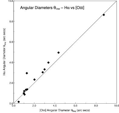
Figure 2: Comparison of H$\alpha$ and [O iii] angular diameters $\theta_{\mathrm{line}}$.

                                       

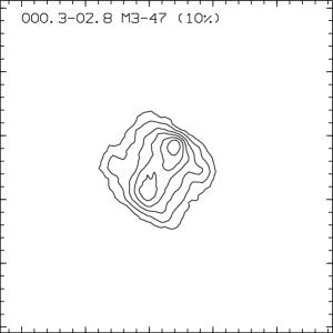
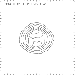
Figure 3: H$\alpha$ images with contour levels at 80, 65, 50, 35, 20, 10, (5, 2, 1, 0.5, 0.2, 0.1) per cent of the nebula peak (lowest indicated after PNe name). All images are 26″ $\times$ 26″ with north up and east to the left. To filter the noise, the images have been smoothed with a 3 pixel (0$\aas@@fstack{\prime\prime}$81) box.

                                       

Figure 3: (continued) H$\alpha$ images with contour levels at 80, 65, 50, 35, 20, 10, (5, 2, 1, 0.5, 0.2, 0.1) per cent of the nebula peak. Actual lowest contour level plotted dependent on signal-to-noise ratio, and indicated after PNe name. The images have been smoothed with a 3 pixel (0$\aas@@fstack{\prime\prime}$81) box.

                                       

Figure 3: (continued) H$\alpha$ images with contour levels at 80, 65, 50, 35, 20, 10, (5, 2, 1, 0.5, 0.2, 0.1) per cent of the nebula peak. Actual lowest contour level plotted dependent on signal-to-noise ratio, and indicated after PNe name. The images have been smoothed with a 3 pixel (0$\aas@@fstack{\prime\prime}$81) box.

     

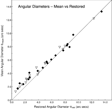
Figure 4: Comparison of H$\alpha$ angular diameters $\theta_{\mathrm{mean}}$ and $\theta_{\mathrm{rest}}$. Diamonds denote major axis diameters, triangles minor axis diameters.

Table 4: Angular diameters of 69 planetary nebulae. Diameters are in arc seconds and are defined in section 3.

PN G	Object	Line	$\theta_{\mathrm{PSF}}{}^{1}$	$\theta_{\mathrm{gauss}}$	$\theta_{\mathrm{shell}}$	$\theta_{\mathrm{line}}$	$\theta_{\mathrm{mean}}$		$\theta_{\mathrm{10\%}}$	$\theta_{\mathrm{rad}}$	$\theta_{\mathrm{opt}}$	AR2	Notes3
000.3$-$04.6	M2-28	H$\alpha$	$1.57\pm 0.03$	4.10	5.3	6.4	5.8	$\pm$ 0.5	9.0 $\times$ 8.0		4.8	1.09	fr, ellip
000.3$-$02.8	M3-47	H$\alpha$	$1.10\pm 0.09$	4.67	5.8	7.1	7.4 $\times$ 5.5	$\pm$ 0.6	9.0 $\times$ 8.0		St.	1.35	fr, irreg
000.6$-$01.3	Bl3-15	H$\alpha$	$1.50\pm 0.03$	2.15	3.0	3.5	3.4 $\times$ 3.1	$\pm$ 0.3	6.0 $\times$ 4.5		3.0	1.08	fr, ellip
000.8$-$01.5	BlO	H$\alpha$	$1.30\pm 0.02$	1.89	2.6	3.1	2.8	$\pm$ 0.2			St.	1.03	fr
002.3$-$03.4	H2-37	H$\alpha$	$1.88\pm 0.02$	2.98	4.0	4.8	5.5 $\times$ 3.2	$\pm$ 0.4	7.0 $\times$ 5.5		4.2	1.54	fr, ellip
002.8$-$02.2	Pe2-12	H$\alpha$	$2.00\pm 0.06$	4.70	6.1	6.6	9.8 $\times$ 3.3	$\pm$ 0.2	10.5 $\times$ 5.0		5.0	2.49	fr, disc
003.0$-$02.6	KFL4	H$\alpha$	$1.81\pm 0.04$	1.46	2.2	2.3	2.2	$\pm$ 0.1			3.0	1.01	pr
003.6$+$03.1	M2-14	H$\alpha$	$1.94\pm 0.08$	1.68	2.5	2.9	3.1 $\times$ 2.2	$\pm$ 0.2		$2.2$	St.	1.17	pr
003.7$-$04.6	M2-30	H$\alpha$	$1.57\pm 0.06$	2.79	3.7	4.5	4.4 $\times$ 3.8	$\pm$ 0.4		$3.5$	9.0	1.12	fr
003.8$-$17.1	Hb8	H$\alpha$	$1.50\pm 0.09$	0.66	1.0	1.2	1.1	$\pm$ 0.1		$0.8$	5.0	1.04	br
004.0$-$11.1	M3-29	H$\alpha$	$1.64\pm 0.07$	5.24	6.7	8.0	7.3	$\pm$ 0.7	10.5 $\times$ 9.5	$13.0$	8.2	1.06	fr, ellip
004.7$-$11.8	He2-418	H$\alpha$	$1.18\pm 0.05$	7.40	9.2	11.1	12.8 $\times$ 7.6	$\pm$ 1.0	14.0 $\times$ 8.5		13.0	1.68	fr, irreg
004.8$-$22.7	He2-436	H$\alpha$	$1.38\pm 0.14$	0.32	0.5	0.6	0.6	$\pm$ 0.0			$<10$	1.05	br
004.8$-$05.0	M3-26	H$\alpha$	$1.54\pm 0.02$	5.93	7.5	8.0	7.7	$\pm$ 0.3	11.0 $\times$ 9.5		8.6	1.03	fr, disc
005.2$-$18.6	StWr2-21	H$\alpha$	$1.80\pm 0.13$	1.40	2.1	2.4	2.5 $\times$ 2.0	$\pm$ 0.2			$<5$	1.10	pr
006.0$-$41.9	PRMG1	H$\alpha$	$1.38^{a}$	2.65	3.5	4.2	4.4 $\times$ 3.3	$\pm$ 0.3			8.2	1.29	fr, irreg
006.8$-$19.8	Wray16-423	H$\alpha$	$1.78\pm 0.12$	1.08	1.6	1.9	1.9 $\times$ 1.6	$\pm$ 0.1			St.	1.05	pr
008.6$-$07.0	He2-406	H$\alpha$	$1.56\pm 0.04$	3.72	4.8	5.8	5.8 $\times$ 4.9	$\pm$ 0.5	8.0 $\times$ 7.5		3.0	1.17	fr, irreg
008.6$-$02.6	MaC1-11	H$\alpha$	$1.82\pm 0.04$	1.97	2.8	3.3	3.3 $\times$ 2.9	$\pm$ 0.2			St.	1.09	pr
009.4$-$09.8	M3-32	H$\alpha$	$1.52\pm 0.04$	4.32	5.5	6.7	6.8 $\times$ 5.4	$\pm$ 0.6	8.5 $\times$ 7.5	$7.5$	6.0	1.24	fr, ring
037.5$-$05.1	A58	[O iii]	$1.77\pm 0.05$	0.70	1.1	1.2	1.4 $\times$ 0.9	$\pm$ 0.0				1.06	br, irreg
283.8$+$02.2	My60	H$\alpha$	$1.65\pm 0.02$	5.65	7.2	8.6	7.9	$\pm$ 0.7	11.0 $\times$ 10.5		7.6	1.07	fr
		[O iii]	$1.97\pm 0.03$	6.43	8.2	8.8	8.5	$\pm$ 0.3	12.5 $\times$ 12.5			1.07	fr
289.8$+$07.7	He2-63	H$\alpha$	$1.47\pm 0.06$	1.83	2.6	3.0	3.0 $\times$ 2.6	$\pm$ 0.2			3.0	1.11	fr
		[O iii]	$1.55\pm 0.03$	1.87	2.6	2.8	3.1 $\times$ 2.6	$\pm$ 0.1				1.12	pr
292.8$+$01.1	He2-67	H$\alpha$	$1.55\pm 0.01$	2.18	3.0	3.6	3.6 $\times$ 3.0	$\pm$ 0.3	6.0 $\times$ 4.5		$<5$	1.16	fr, ellip
296.4$-$06.9	He2-71	[O iii]	$2.04\pm 0.20$	0.36	0.6	0.6	0.6	$\pm$ 0.0				1.08	br
305.1$+$01.4	He2-90	H$\alpha$	$1.39\pm 0.04$	0.48	0.8	0.9	0.8	$\pm$ 0.1			$<10$	1.01	br
		[O iii]	$1.71\pm 0.01$	0.63	1.0	1.1	1.3 $\times$ 0.8	$\pm$ 0.0				1.06	br
315.4$+$09.4	He2-104	H$\alpha$	$1.73\pm 0.05$	0.40	0.6	0.7	0.7	$\pm$ 0.0			$<5$	1.02	br, outflow
321.3$-$16.7	He2-185	H$\alpha$	$1.73\pm 0.06$	1.53	2.2	2.6	2.8 $\times$ 2.0	$\pm$ 0.2			$<5$	1.17	pr
322.4$-$00.1	Pe2-8	H$\alpha$	$1.68\pm 0.06$	0.97	1.5	1.7	1.9 $\times$ 1.3	$\pm$ 0.1			1.6	1.09	pr
345.0$-$04.9	Cn1-3	H$\alpha$	$1.48\pm 0.02$	0.74	1.2	1.3	1.2	$\pm$ 0.1			$<5$	1.02	br
		[O iii]	$1.75\pm 0.01$	0.71	1.1	1.2	1.2	$\pm$ 0.0				1.02	br
345.0$+$03.4	Vd1-4	H$\alpha$	$1.79\pm 0.03$	0.66	1.0	1.2	1.1	$\pm$ 0.1			5.0	1.03	br
		[O iii]	$1.62\pm 0.03$	0.61	1.0	1.0	1.0	$\pm$ 0.0				1.03	br
345.0$+$04.3	Vd1-2	H$\alpha$	$1.86\pm 0.01$	0.76	1.2	1.4	1.3	$\pm$ 0.1			St.	1.00	br, diffuse
		[O iii]	$1.70\pm 0.03$	0.79	1.2	1.3	1.3	$\pm$ 0.0				1.70	br
346.0$+$08.5	He2-171	H$\alpha$	$1.01\pm 0.03$	0.08	0.1	0.2	0.1	$\pm$ 0.0			$<10$	1.04	br
		[O iii]	$1.10\pm 0.07$	0.28	0.5	0.5	0.5	$\pm$ 0.0				1.00	br
346.3$-$06.8	Fg2	H$\alpha$	$1.17\pm 0.04$	3.20	4.1	5.0	4.9 $\times$ 4.2	$\pm$ 0.4	6.5 $\times$ 5.5		$<5$	1.14	fr
		[O iii]	$1.13\pm 0.03$	3.17	4.1	4.4	4.8 $\times$ 4.2	$\pm$ 0.1				1.13	fr
347.4$+$05.8	H1-2	H$\alpha$	$1.14\pm 0.02$	0.55	0.9	1.0	1.1 $\times$ 0.8	$\pm$ 0.1		$0.8$	St.	1.07	br
		[O iii]	$1.26\pm 0.03$	0.59	0.9	1.0	1.2 $\times$ 0.8	$\pm$ 0.0				1.07	br
348.0$+$06.3	MGP1	H$\alpha$	$1.98\pm 0.14^{c}$	4.92	6.4	7.7	7.6 $\times$ 6.4	$\pm$ 0.6	12.0 $\times$ 9.5	$3.8$		1.17	fr, ellip
348.8$-$09.0	He2-306	H$\alpha$	$1.40\pm 0.02$	2.04	2.8	3.3	3.1	$\pm$ 0.3			3.0	1.07	fr
		[O iii]	$1.57\pm 0.01$	2.01	2.8	3.0	2.9	$\pm$ 0.1				1.06	pr
349.8$+$04.4	M2-4	H$\alpha$	$1.12\pm 0.02$	1.40	2.0	2.3	2.1	$\pm$ 0.2		$2.0$	$<5$	1.09	fr, ellip
		[O iii]	$1.21\pm 0.03$	1.32	1.9	2.0	2.0	$\pm$ 0.1				1.07	pr
350.8$-$02.4	H1-22	H$\alpha$	$2.13\pm 0.09$	2.17	3.1	3.7	3.4	$\pm$ 0.3			St.	1.01	pr
350.9$+$04.4	H2-1	H$\alpha$	$1.38\pm 0.03$	1.79	2.5	2.9	2.7	$\pm$ 0.2		$2.2$	5.6	1.00	fr
		[O iii]	$1.32\pm 0.04$	0.78	1.2	1.3	1.2	$\pm$ 0.0				1.01	br
351.1$+$04.8	M1-19	H$\alpha$	$1.32\pm 0.02$	1.99	2.7	3.2	3.2 $\times$ 2.7	$\pm$ 0.3		$2.6$	8.0	1.13	fr
351.2$+$05.2	M2-5	H$\alpha$	$1.33\pm 0.01$	3.41	4.4	5.3	4.9	$\pm$ 0.4	6.5 $\times$ 6.5	$5.0$	5.0	1.03	fr, outflow
351.3$+$07.6	H1-4	H$\alpha$	$1.51\pm 0.02$	0.64	1.0	1.2	1.1	$\pm$ 0.1			St.	1.02	br
351.9$-$01.9	Wray16-286	H$\alpha$	$1.69\pm 0.06$	1.16	1.8	2.0	2.2 $\times$ 1.6	$\pm$ 0.1			St.	1.12	pr, ellip
351.9$+$09.0	PC13	H$\alpha$	$2.07\pm 0.04$	5.15	6.7	8.0	8.6 $\times$ 6.0	$\pm$ 0.7	10.0 $\times$ 8.5		7.0	1.39	fr, disc
352.0$-$04.6	H1-30	H$\alpha$	$1.78\pm 0.05$	1.63	2.4	2.8	3.0 $\times$ 2.1	$\pm$ 0.2			5.4	1.20	pr, ellip

¹ Error expressed as the standard deviation of four $\theta_{\mathrm{PSF}}$ values except: ^aone value, ^btwo values, ^cthree values.

² Maximum/minimum axis ratio of planetary nebulae from 2D FWHM measurements.

³ br, barely resolved, $\theta_{\mathrm{line}}<\theta_{\mathrm{PSF}}$; pr, partly resolved, $\theta_{\mathrm{PSF}}<\theta_{\mathrm{line}}<2\theta_{\mathrm{PSF}}$; fr, fully resolved, $\theta_{\mathrm{line}}\geq 2\theta_{\mathrm{PSF}}$.

Table 4: (continued) Angular diameters of 69 planetary nebulae. Diameters are in arc seconds and are defined in section 3.

PN G	Object	Line	$\theta_{\mathrm{PSF}}{}^{1}$	$\theta_{\mathrm{gauss}}$	$\theta_{\mathrm{shell}}$	$\theta_{\mathrm{line}}$	$\theta_{\mathrm{mean}}$		$\theta_{\mathrm{10\%}}$	$\theta_{\mathrm{rad}}$	$\theta_{\mathrm{opt}}$	AR2	Notes3
352.1$+$05.1	M2-8	H$\alpha$	$1.10\pm 0.01$	2.55	3.3	4.0	3.8 $\times$ 3.5	$\pm$ 0.3	5.0 $\times$ 5.0	$3.7$	4.2	1.10	fr, outflow
		[O iii]	$1.24\pm 0.04$	2.37	3.2	3.4	3.3	$\pm$ 0.1				1.05	fr, outflow
352.6$+$00.1	H1-12	H$\alpha$	$1.13\pm 0.03$	5.76	7.2	8.7	7.9	$\pm$ 0.8	12.0 $\times$ 10.0	$11.0$	6.8	1.00	fr
352.6$+$03.0	H1-8	H$\alpha$	$1.36\pm 0.02$	1.92	2.6	3.1	3.1 $\times$ 2.6	$\pm$ 0.2			3.4	1.14	fr
352.8$-$00.2	H1-13	H$\alpha$	$1.57\pm 0.16^{c}$	9.27	11.5	14.0	12.7	$\pm$ 1.2	13.5 $\times$ 12.0	$14.0$	9.6	1.08	fr, ring
354.2$+$04.3	M2-10	H$\alpha$	$1.64\pm 0.03$	2.93	3.9	4.7	5.2 $\times$ 3.4	$\pm$ 0.4	6.5 $\times$ 5.5	$4.0$	4.0	1.42	fr, irreg
354.5$+$03.3	Th3-4	H$\alpha$	$1.84\pm 0.11$	0.97	1.5	1.7	2.0 $\times$ 1.2	$\pm$ 0.1			St.	1.12	br
354.9$+$03.5	Th3-6	H$\alpha$	$2.38\pm 0.08$	2.49	3.6	4.2	4.1 $\times$ 3.7	$\pm$ 0.3			St.	1.07	pr
355.1$-$06.9	M3-21	H$\alpha$	$1.51\pm 0.02$	1.00	1.5	1.8	1.8 $\times$ 1.5	$\pm$ 0.1			$<5$	1.08	pr
355.1$+$02.3	Th3-11	H$\alpha$	$1.42\pm 0.04$	1.21	1.8	2.1	2.1 $\times$ 1.7	$\pm$ 0.2			St.	1.10	pr
355.4$-$02.4	M3-14	H$\alpha$	$1.52\pm 0.02$	2.40	3.3	3.9	3.6	$\pm$ 0.3	8.0 $\times$ 5.0	$2.8$	7.2	1.01	fr, ellip
355.7$-$03.5	H1-35	H$\alpha$	$1.40\pm 0.04$	0.90	1.4	1.6	1.5	$\pm$ 0.1		$1.1$	2.0	1.07	pr
355.9$+$02.7	Th3-10	H$\alpha$	$1.24\pm 0.03$	1.58	2.2	2.6	2.4	$\pm$ 0.2		$2.0$	St.	1.07	fr
356.1$+$02.7	Th3-13	H$\alpha$	$1.63\pm 0.02$	0.45	0.7	0.8	1.1 $\times$ 0.2	$\pm$ 0.1		$<2$	St.	1.07	br
356.8$+$03.3	Th3-12	H$\alpha$	$1.75\pm 0.13$	1.22	1.8	2.1	2.3 $\times$ 1.6	$\pm$ 0.1		$1.2$	St.	1.12	pr
357.1$-$06.1	M3-50	H$\alpha$	$1.25\pm 0.04$	3.06	4.0	4.8	6.7 $\times$ 1.7	$\pm$ 0.4	8.5 $\times$ 3.5		4.0	3.03	fr, disc
357.1$-$04.7	H1-43	H$\alpha$	$1.71\pm 0.03$	0.91	1.4	1.6	1.7 $\times$ 1.3	$\pm$ 0.1		$3.0$	2.0	1.08	br
357.1$+$01.9	Th3-24	H$\alpha$	$1.24\pm 0.04$	4.61	5.8	7.0	6.4	$\pm$ 0.6	8.0 $\times$ 7.0		St.	1.07	fr, irreg
357.1$+$03.6	M3-7	H$\alpha$	$1.39\pm 0.02$	3.15	4.1	4.9	4.9 $\times$ 4.1	$\pm$ 0.4	6.5 $\times$ 5.5	$4.7$	5.8	1.18	fr
357.6$-$03.3	H2-29	H$\alpha$	$1.45\pm 0.02$	7.31	9.1	11.0	12.5 $\times$ 7.7	$\pm$ 1.0			4.8	1.61	fr, irreg
358.5$+$03.7	Al2-B	H$\alpha$	$1.56\pm 0.04$	1.62	2.3	2.7	3.0 $\times$ 2.1	$\pm$ 0.2			St.	1.22	pr, irreg
358.5$-$01.7	JaSt64	H$\alpha$	$1.19\pm 0.05$	0.98	1.5	1.7	1.6	$\pm$ 0.1				1.04	pr
358.7$+$05.2	M3-40	H$\alpha$	$1.49\pm 0.12^{b}$	1.96	2.7	3.2	3.0	$\pm$ 0.3		$2.5$	St.	1.05	fr
359.2$+$04.7	Th3-14	H$\alpha$	$1.48\pm 0.05$	1.15	1.7	2.0	1.9	$\pm$ 0.1		$<3.3$		1.03	pr

¹ Error expressed as the standard deviation of four $\theta_{\mathrm{PSF}}$ values except: ^aone value, ^btwo values, ^cthree values.

² Maximum/minimum axis ratio of planetary nebulae from 2D FWHM measurements.

³ br, barely resolved, $\theta_{\mathrm{line}}<\theta_{\mathrm{PSF}}$; pr, partly resolved, $\theta_{\mathrm{PSF}}<\theta_{\mathrm{line}}<2\theta_{\mathrm{PSF}}$; fr, fully resolved, $\theta_{\mathrm{line}}\geq 2\theta_{\mathrm{PSF}}$.

Table 5: Flux and extinction values of 70 planetary nebulae. Observed (equation 7) and catalogue (equation 10) extinction are defined in section 5.

PN G	Object	Line	Radial Vel. (km s-1)		Flux (log mW m-2)		S$\nu$ 6 cm	H$\alpha$ Extinction		$R_{\mathrm{V}}$	$\Delta R_{\mathrm{V}}$	Notes5
			Observed	Catalogue	Observed	Catalogue	(mJy)4	Observed	Catalogue
000.3$-$04.6	M2-28	H$\alpha$	$-43.5$	$-29.9$	$-11.70$	$-11.73$	$10$	$0.66$	$0.98$	$1.99$	$0.62$	B
000.3$-$02.8	M3-47	H$\alpha$	$-17.9$	$-16.0$	$-12.47$	$-12.88$			$1.58$
000.6$-$01.3	Bl3-15	H$\alpha$	$-114.8$		$-12.59$	$-12.92$			$2.89$
000.8$-$01.5	BlO	H$\alpha$	$79.9$		$-12.18$	$-11.82$			$2.04$
002.3$-$03.4	H2-37	H$\alpha$	$-129.8$	$-156.8$	$-11.86$	$-12.06$			$0.69$
002.8$-$02.2	Pe2-12	H$\alpha$	$108.8$		$-11.86$	$-12.46$	$2$	$0.13$	$1.06$	$0.57$	$0.41$	lrf
003.0$-$02.6	KFL4	H$\alpha$	$-12.9$	$17.0$	$-12.59$	$-12.81$	$1$	$0.59$	$1.02$	$1.71$	$0.56$	lrf
003.6$+$03.1	M2-14	H$\alpha$	$-25.0$	$-48.2$	$-11.35$	$-12.15$	$39$	$0.90$	$1.41$	$1.87$	$0.42$	B
003.7$-$04.6	M2-30	H$\alpha$	$130.0$	$154.9$	$-11.29$	$-11.18$	$14$	$0.40$	$0.74$	$1.59$	$0.75$	B
003.8$-$17.1	Hb8	H$\alpha$	$-170.1$	$-180.5$	$-11.30$	$-11.28$	$6$	$0.03$	$0.20$	$0.64$	$2.30$	lrf
004.0$-$11.1	M3-29	H$\alpha$	$26.2$	$49.3$	$-11.20$	$-11.10$	$12$	$0.25$	$0.12$	$10.81$	$31.50$	B
004.7$-$11.8	He2-418	H$\alpha$	$87.7$	$109.3$	$-12.05$	$-11.90$			$0.12$
004.8$-$22.7	He2-436	H$\alpha$	$128.4$	$133.0$	$-11.86$	$-11.50$	${\bf 3}.{\bf 9}$	$0.41$	$0.50$	$2.45$	$1.36$	lrf
004.8$-$05.0	M3-26	H$\alpha$	$-24.7$	$-9.8$	$-11.41$	$-11.26$	$8$	$0.28$	$0.43$	$1.90$	$1.40$	lrf
005.2$-$18.6	StWr2-21	H$\alpha$	$136.3$	$133.0$	$-12.26$	$-12.46$			$0.32$
006.0$-$41.9	PRMG1	H$\alpha$	$-8.1$		$-12.95$	$-12.77$			$0.18$
006.8$-$19.8	Wray16-423	H$\alpha$	$139.2$	$133.0$	$-11.78$	$-11.48$	${\bf 4}.{\bf 7}$	$0.42$	$0.36$	$3.78$	$2.47$	lrf
008.6$-$07.0	He2-406	H$\alpha$	$-8.5$	$28.2$	$-12.12$	$-12.38$			$0.84$
008.6$-$02.6	MaC1-11	H$\alpha$	$-30.8$	$-89.0$	$-12.33$	$-12.25$			$1.76$
009.4$-$09.8	M3-32	H$\alpha$	$40.1$	$58.4$	$-11.39$	$-11.22$	$12$	$0.43$	$0.53$	$2.46$	$1.29$	B
009.8$-$07.5	GJJC1	[O iii]		$-32.0$	$-12.74$
037.5$-$05.1	A58	H$\alpha$		$70.0$	$-13.40$
		[O iii]			$-12.91$
283.8$+$02.2	My60	H$\alpha$			$\geq-11.53$	$-11.04$	$60$	$\leq 1.27$	$0.67$			npc
		[O iii]			$\geq-10.68$	$-10.64$

⁴ Bold values are for PNe in the Sagittarius dwarf galaxy (Dudziak et al., 2000). All other values from the Strasbourg - ESO Catalogue (Acker et al., 1992).

⁵ B, Bulge subset B; npc, non-photometric conditions; hbt, high brightness temperature, $T_{\mathrm{b}}>$ 1000 K; lrf, low radio flux, $S_{\nu}<$ 10 mJy.

Table 5: (continued) Flux and extinction values of 70 planetary nebulae. Observed (equation 7) and catalogue (equation 10) extinction are defined in section 5.

PN G	Object	Line	Radial Vel. (km s-1)		Flux (log mW m-2)		S$\nu$ 6 cm	H$\alpha$ Extinction		$R_{\mathrm{V}}$	$\Delta R_{\mathrm{V}}$	Notes5
			Observed	Catalogue	Observed	Catalogue	(mJy)4	Observed	Catalogue
289.8$+$07.7	He2-63	H$\alpha$		$123.2$	$\geq-11.92$	$-11.91$	$12$	$\leq 0.96$	$0.27$			npc
		[O iii]			$\geq-11.14$	$-11.43$
292.8$+$01.1	He2-67	H$\alpha$		$59.5$	$\geq-12.47$	$-11.17$	$41$	$\leq 1.51$	$0.83$			npc
296.4$-$06.9	He2-71	[O iii]			$\geq-11.71$	$-11.69$						npc
305.1$+$01.4	He2-90	H$\alpha$			$\geq-10.71$	$-10.52$	$25$		$1.13$			hbt
		[O iii]			$\geq-10.73$	$-11.14$
315.4$+$09.4	He2-104	H$\alpha$	$-70.4$	$-143.6$	$-10.83$	$-10.81$	$<15$		$1.09$			hbt
321.3$-$16.7	He2-185	H$\alpha$	$-12.0$	$-6.0$	$-11.10$	$-10.97$	$18$	$0.32$	$0.20$	$6.24$	$7.24$
322.4$-$00.1	Pe2-8	H$\alpha$	$-23.9$	$-16.3$	$-11.95$	$-11.96$	$100$	$\geq 1.91$	$3.16$	$1.78$	$0.18$	hbt
345.0$-$04.9	Cn1-3	H$\alpha$	$-68.2$	$-79.8$	$\geq-10.89$	$-10.58$			$0.13$			npc
		[O iii]			$\geq-10.71$	$-10.33$						npc
345.0$+$03.4	Vd1-4	H$\alpha$	$93.4$	$35.1$	$-12.11$	$-12.18$			$0.84$
		[O iii]			$-11.73$	$-11.80$
345.0$+$04.3	Vd1-2	H$\alpha$		$3.4$	$-11.57$	$-12.30$			$1.16$
		[O iii]			$-13.08$
346.0$+$08.5	He2-171	H$\alpha$	$-100.2$	$-101.5$	$\geq-11.69$	$-11.09$	$10$		$1.54$			hbt
		[O iii]			$\geq-11.94$	$-11.64$
346.3$-$06.8	Fg2	H$\alpha$	$52.5$	$34.5$	$-11.12$	$-11.19$			$0.37$
		[O iii]			$-10.47$	$-10.59$
347.4$+$05.8	H1-2	H$\alpha$	$-124.8$	$-105.5$	$-11.02$	$-10.96$	$62$	$\geq 0.78$	$1.57$	$\geq 1.47$	$0.34$	hbt
		[O iii]			$-10.72$	$-11.24$
348.0$+$06.3	MGP1	H$\alpha$	$-67.9$	$-52.0$	$-12.15$		$10.2$	$1.12$
348.8$-$09.0	He2-306	H$\alpha$	$-49.6$	$-40.0$	$-11.14$	$-11.23$			$0.27$
		[O iii]			$-11.00$	$-11.14$
349.8$+$04.4	M2-4	H$\alpha$	$-227.0$	$-207.2$	$-11.06$	$-10.93$	$32$	$0.53$	$1.08$	$1.47$	$0.50$	B
		[O iii]			$-10.97$	$-10.94$
350.8$-$02.4	H1-22	H$\alpha$	$-199.6$	$-213.0$	$-11.76$	$-11.72$			$1.66$
350.9$+$04.4	H2-1	H$\alpha$	$-35.5$	$-18.8$	$-10.62$	$-10.67$	$61$	$0.37$	$0.79$	$1.38$	$0.67$	B
		[O iii]			$-11.57$	$-11.63$
351.1$+$04.8	M1-19	H$\alpha$	$-68.6$	$-55.2$	$-11.10$	$-11.15$	$26$	$0.48$	$0.93$	$1.53$	$0.59$	B
351.2$+$05.2	M2-5	H$\alpha$	$-134.6$	$-123.4$	$-11.18$	$-11.26$	$12$	$0.22$	$0.90$	$0.84$	$0.52$	B
351.3$+$07.6	H1-4	H$\alpha$	$10.1$	$2.7$	$-11.88$	$-11.57$			$0.52$
351.9$-$01.9	Wray16-286	H$\alpha$	$-143.9$	$-152.3$	$-11.79$	$-11.82$			$1.91$
351.9$+$09.0	PC13	H$\alpha$		$-75.1$	$-11.63$	$-11.54$			$0.73$
352.0$-$04.6	H1-30	H$\alpha$	$5.6$	$-12.9$	$-12.01$	$-12.12$			$1.30$
352.1$+$05.1	M2-8	H$\alpha$	$18.2$	$25.1$	$-11.31$	$-11.72$	$18$	$0.53$	$0.78$	$1.99$	$0.79$	B
		[O iii]			$-11.11$	$-11.52$
352.6$+$00.1	H1-12	H$\alpha$			$-11.85$	$-12.10$	$>719$	$2.67$	$3.88$	$2.02$	$0.16$
352.6$+$03.0	H1-8	H$\alpha$	$-3.9$	$-116.0$	$-11.97$	$-11.91$			$2.32$
352.8$-$00.2	H1-13	H$\alpha$	$-11.6$	$-26.3$	$-11.48$	$-11.65$	$>620$	$2.23$	$2.60$	$2.59$	$0.27$
354.2$+$04.3	M2-10	H$\alpha$	$-64.2$	$-85.6$	$-11.58$	$-11.61$	$9.1$	$0.50$	$1.31$	$1.17$	$0.38$	lrf
354.5$+$03.3	Th3-4	H$\alpha$	$-122.9$	$-165.0$	$-12.26$	$-12.03$			$2.15$
354.9$+$03.5	Th3-6	H$\alpha$	$-92.5$	$-73.1$	$-12.28$	$-12.40$			$1.93$
355.1$-$06.9	M3-21	H$\alpha$	$-78.6$	$-66.9$	$-10.84$	$-10.93$	$30$	$0.28$	$0.08$	$276.33$	$42.22$	B
355.1$+$02.3	Th3-11	H$\alpha$	$-33.1$		$-12.81$
355.4$-$02.4	M3-14	H$\alpha$	$-63.3$	$-82.3$	$-11.47$	$-11.33$	$30$	$0.91$	$1.45$	$1.85$	$0.41$	B
355.7$-$03.5	H1-35	H$\alpha$	$135.1$	$123.4$	$-10.92$	$-10.58$	$72$	$\geq 0.74$	$0.98$	$\geq 2.24$	$0.66$	hbt
355.9$+$02.7	Th3-10	H$\alpha$	$-256.5$		$-12.70$	$-12.96$	$29.5$	$2.14$	$2.55$	$2.51$	$0.27$	B
356.1$+$02.7	Th3-13	H$\alpha$	$-75.3$	$-99.0$	$-12.31$	$-12.20$	$14.3$	$\geq 1.43$	$2.69$	$\geq 1.56$	$0.21$	hbt
356.8$+$03.3	Th3-12	H$\alpha$	$248.8$	$185.4$	$-12.61$	$-12.63$	$3.5$	$1.12$	$1.56$	$2.12$	$0.40$	lrf
357.1$-$06.1	M3-50	H$\alpha$	$26.4$	$17.5$	$-12.26$	$-12.29$			$0.51$
357.1$-$04.7	H1-43	H$\alpha$	$44.9$	$49.0$	$-11.55$	$-11.67$	$6$	$0.29$	$0.93$	$0.99$	$0.52$	lrf
357.1$+$01.9	Th3-24	H$\alpha$	$-152.4$	$-197.0$	$-12.76$	$-13.08$			$1.57$
357.1$+$03.6	M3-7	H$\alpha$	$-171.7$	$-193.6$	$-11.34$	$-11.33$	$28$	$0.75$	$1.20$	$1.84$	$0.49$	B
357.6$-$03.3	H2-29	H$\alpha$	$123.4$	$107.0$	$-12.38$	$-12.79$			$1.30$
358.5$+$03.7	Al2-B	H$\alpha$	$-134.0$	$-158.0$	$-12.97$
358.5$-$01.7	JaSt64	H$\alpha$	$17.6$		$-13.13$
358.7$+$05.2	M3-40	H$\alpha$	$54.0$	$32.8$	$-12.25$	$-12.23$	$15.1$	$1.39$	$1.93$	$2.13$	$0.33$	B
359.2$+$04.7	Th3-14	H$\alpha$	$-206.7$	$-239.2$	$-12.20$	$-12.27$	$4$	$0.77$	$1.54$	$1.48$	$0.35$	lrf

⁵ B, Bulge subset B; npc, non-photometric conditions; hbt, high brightness temperature, $T_{\mathrm{b}}>$ 1000 K; lrf, low radio flux, $S_{\nu}<$ 10 mJy.

3.4 Discussion

By their nature PNe at a given distance are likely to exhibit a range of angular diameters depending on where they are in their evolutionary sequence of returning shed material from the proginator star to the ISM. This is in addition to observed angular size differences for the same source, e.g. optical versus radio or specific line emission.

It is apparent from a visual inspection of our images that not all PNe have a well-defined outer radius. For such soft boundary PNe a 10 per cent radius does not have a direct physical meaning and usually does not correlate well with converted deconvolved FWHM diameters. This is not surprising as 10 per cent (or lower if signal-to-noise will allow) radius measurements ‘see’ into the extended low emission regions surrounding PNe, whereas FWHM determinations tend to reveal the compact core. These differing values actually give us alternative views of a PNe’s morphology and tell us more about the object than a single arbitrary radius value.

4 Flux determinations

4.1 Method

The total flux detected is reduced by the transmission of the H$\alpha$ and [O iii] filters. This and other factors must be taken into account when determining actual flux values, and we now describe the methods used to arrive at the values listed in Table 5.

The central position of each object was computed by fitting a Gaussian to the image distribution and then the magnitude was calculated by integrating over successively larger diameters of the central area. By plotting these radii against magnitude it was possible to determine the radius at which the flux level matched that of the background continuum, and therefore the total flux of the object in ADU counts per 30 second exposure. These profiles were compared with those of standard stars LTT1020 and LTT624 to determine the aperture correction.

To determine detector flux values in mW m^-2 (erg cm^-2s^-1), the ratio of ADU count to flux conversion factor was calculated by measuring the count in ADUs per ten seconds of LTT1020 and LTT6248, and comparing it with tabulated fluxes for these spectrophotometric standards (Hamuy et al., 1994). The calibration counts were factored for the shorter exposure time, and the aperture correction of $-$5 per cent was applied. Apart from a brief period of non-photometric conditions caused by cloud (indicated as ‘npc’ in Table 5), observations were considered photometric as the computed ADU count to flux ratios varied by no more than 2.1 per cent between the two night’s observations.

In order to determine actual H$\alpha$ 6565Å flux values, any contribution from [N ii] lines at 6548Å and 6584Å (vacuum), passing through ESO filter #654, was taken into account by assuming the following expression for the total detected flux:

$$F_{\mathrm{det}}=F_{6565}T_{6565}+F_{6584}T_{6584}+F_{6548}T_{6548}$$ (3)

where $F\lambda$ and $T\lambda$ are actual flux values and filter transmission coefficients (corrected for the appropriate Doppler shift) respectively. Using catalogue [N ii] to H$\alpha$ flux ratios $R_{6584}=F_{6584}/F_{6565}$ and $R_{6548}=F_{6548}/F_{6565}$ (which avoid a dependence on absolute values), the actual H$\alpha$ 6565Å flux can be calculated using:

$$F(\mathrm{H\alpha)_{obs}}=F_{\mathrm{det}}/(T_{6565}+R_{6584}T_{6584}+R_{6548}T_{6548})$$ (4)

[N ii]₆₅₄₈ flux values were calculated from the [N ii]₆₅₈₄ catalogue values (Acker et al., 1992) using a factor of 2.97. In the case of [O iii], the flux observed through the filter was factored for the appropriate transmission coefficient of the [O iii] wavelength, so as to arrive at actual observed [O iii] flux values.

The Doppler shifted H$\alpha$ and [O iii] wavelengths observed at the telescope were computed from catalogue radial velocities (Durand et al., 1998; Acker et al., 1992) less a barycentric correction appropriate to the date and time at La Silla, or in the absence of a catalogue value, derived from spectra taken during our observations. Columns four and five of Table 5 compare catalogue radial velocities with observed values, which we consider accurate to $\pm$25 km s^-1. For three objects it was not possible to determine the radial velocity at all. Using the corrected filter response curves (measured at La Silla air pressure), the appropriate transmission coefficient was then applied to arrive at actual flux values. La Silla-air wavelengths were 6563.3Å for H$\alpha$ and 5007.3Å for [O iii], with 6548.5Å and 6583.9Å assumed for [N ii] using the same $\Delta\lambda$ as that of H$\alpha$. Although stellar velocities in the Bulge are typically of the order of $\pm$100 km s^-1 (Minniti, 1996), or about $\pm 2$Å, we have chosen to calculate precise Doppler wavelength shifts, in order to take into account the sensitivity of the H$\alpha$ filter transmission curve to small changes in observed wavelength.

4.2 Results and error factors

 

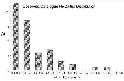
Figure 5: Distribution of $\Delta F(\mathrm{H}\alpha)$, the absolute difference between observed and catalogued H$\alpha$ flux values (log mW m^-2).

Table 5 lists the newly determined H$\alpha$ and [O iii] flux densities in column six. For comparison columns seven and eight list H$\alpha$ and [O iii] flux values (calculated from catalogued H$\beta$ flux and line intensities) and the 6 cm radio flux values from the Strasbourg - ESO Catalogue (Acker et al., 1992). Radio values in bold are for the two PNe in the Sagittarius dwarf galaxy (from Dudziak et al., 2000). Fig. 5 shows the distribution of $\Delta F(\mathrm{H}\alpha)$, the absolute difference between observed and catalogued H$\alpha$ flux values. 7 out of 60 objects are shown to have $\Delta F(\mathrm{H}\alpha)>0.4$ (log mW m^-2). A comparison of $\Delta F(\mathrm{H}\alpha)$ with $\theta_{\mathrm{line}}$ shows no evidence of a correlation between these flux differences and angular diameter.

Fig. 6 compares observed and catalogued H$\alpha$ and [O iii] flux values. Four (non-Bulge) objects (indicated in Table 5) are excluded from Figs. 5 & 6 because atmospheric conditions for those exposures were non-photometric. It can be seen that there is little evidence of any systematic differences between observed and catalogued flux values.

           

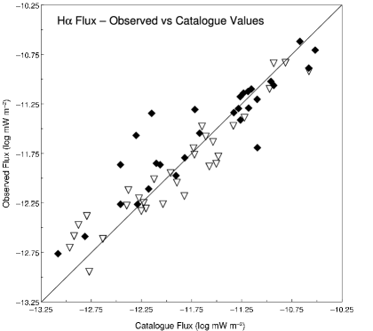
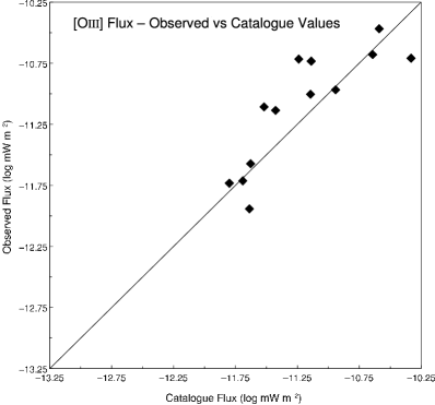
Figure 6: Comparison of observed and catalogued H$\alpha$ and [O iii] flux values (log mW m^-2). Diamonds denote objects observed on the first night, triangles the second.

Possible sources of error in our flux determinations are: poor photometry; residual stellar background flux after subtraction of the continuum; an off-centred peak in the H$\alpha$ on-band filter response curve; estimation of the flux contribution from [N ii] lines; the accuracy of transmission coefficients in the corrected filter response tables (particularly for H$\alpha$); change in passbands of filters due to their age, input beam and ambient temperature; integrating the transmission profile of the filter response curves; uncertainties in radial velocities; changes in air pressure (airmass); and the aperture correction factor. Of these, we consider the accuracy of the filter response data the most significant and therefore suggest an error factor in the calculated flux values (mW m^-2) of $\pm$5 per cent for blue-shifted objects and $\pm$10 per cent for red-shifted objects.

5 Extinction determinations

5.1 Method

Observed H$\alpha$ flux values are reduced from emitted flux values by interstellar extinction. By comparing these observed values with catalogued optical and radio fluxes, extinction values can be determined, and we now describe the methods used to arrive at the values listed in Table 5.

From Pottasch (1984, hereafter SP) the radio to H$\beta$ flux ratio is $S_{\nu}/F(\mathrm{H}\beta)=2.51\times 10^{7}T_{\mathrm{e}}^{0.53}\nu^{-0.1}Y$ (Jy/mW m^-2) where $T_{\mathrm{e}}$ is the electron temperature in K, $\nu$ is the radio frequency in GHz and $Y$ is a factor incorporating the ionized He/H ratio. Setting $T_{\mathrm{e}}=10^{4}$ K, $\nu=5$ GHz, $Y=1.1$ and converting to mJy gives

$$S_{\nu}(6\mathrm{cm})/F(\mathrm{H}\beta)_{\mathrm{0}}=3.10\times 10^{12}\;(\mathrm{mJy/mW\,m}^{-2}).$$ (5)

H$\beta$ extinction ($C_{\beta}$) can be defined as the ratio of expected to observed H$\beta$ flux:

$$C_{\beta}=\log[F(\mathrm{H}\beta)_{\mathrm{0}}/F(\mathrm{H}\beta)]$$ (6)

If an electron density of $n_{\mathrm{e}}=10^{4}$ cm^-3 is assumed, and $T_{\mathrm{e}}=10^{4}$ K, the Balmer-line intensity ratio, $F(\mathrm{H}\alpha)/F(\mathrm{H}\beta)=2.85$. Combining this factor with equations (5) & (6) gives an expression for observed H$\alpha$ extinction in terms of the observed H$\alpha$ flux (mW m^-2) and the (catalogue) radio flux (mJy):

$$C_{\alpha}=\log[2.85S_{\nu}(6\mathrm{cm})/3.10\times 10^{12}F(\mathrm{H}\alpha)].$$ (7)

In order to compare observed versus catalogue extinction values, the latter can be derived from just the catalogue H$\alpha$ and H$\beta$ flux values. We assume that the $F(\mathrm{H}\alpha)/F(\mathrm{H}\beta)$ ratio in the catalogue is accurate, even if the absolute fluxes are in doubt. We start with the full form of equation 6:

$$C_{\beta}=\log[F(\mathrm{H}\beta)_{\mathrm{0}}/F(\mathrm{H}\beta)]=A_{4861}E_{B-V}/2.5$$ (8)

where $A_{\lambda}$ is a wavelength dependent extinction coefficient. It follows that

$$C_{\alpha}=\log[F(\mathrm{H}\alpha)_{\mathrm{0}}/F(\mathrm{H}\alpha)]=A_{6561}E_{B-V}/2.5$$ (9)

Combining equations 8 & 9 with the Balmer-line intensity ratio of 2.85 gives an expression for calculating H$\alpha$ extinction values in terms of catalogue H$\alpha$ and H$\beta$ flux values:

$$C_{\alpha_{\mathrm{opt}}}=B\log[F(\mathrm{H}\alpha)_{\mathrm{cat}}/2.85F(\mathrm{H}\beta)_{\mathrm{cat}}],$$ (10)

where $B=A_{6561}/(A_{4861}-A_{6561})=2.28$ (using data from SP table V-1).

An alternate method of calculating the wavelength dependent constant $B$ in equation 10 is provided by Cardelli, Clayton & Mathis (1989, hereafter CCM) in terms of what they consider a more fundamental extinction law $A(\lambda)/A(V)$, where $A(\lambda)$ is the absolute extinction at $\lambda$ and $A(V)$ is the visual extinction. Based on empirical data, CCM provide a mean $R_{\mathrm{V}}\,[=A(V)/E(B-V)]$ extinction law with wavelength dependent coefficients ($x=\lambda^{-1}\mu\mathrm{m}^{-1}$) that takes the form

$$\langle A(\lambda)/A(V)\rangle=a(x)+b(x)/R_{\mathrm{V}},$$ (11)

where $R_{\mathrm{V}}$ is the ratio of total to selective extinction. Dividing the expression for $B$ by $A(V)$ and substituting the expression $a(x)+b(x)/R_{\mathrm{V}}$ gives

$$B=\frac{(a_{\alpha}+b_{\alpha}/R_{\mathrm{V}})}{(a_{\beta}+b_{\beta}/R_{\mathrm{V}})-(a_{\alpha}+b_{\alpha}/R_{\mathrm{V}})},$$ (12)

where $a_{\alpha}=a(1/\lambda_{\mathrm{H\alpha}})$, $a_{\beta}=a(1/\lambda_{\mathrm{H\beta}})$, etc. Using $R_{\mathrm{V}}=3.1$ and appropriate values provided by CCM (eqs. 3a & 3b) for this polynomial in $x$ gives $B=2.36$, which is slightly higher than SP’s value of $2.28$. However, $B$ is now dependent on the value of $R_{\mathrm{V}}$ so equation 10 takes the $R_{\mathrm{V}}$ dependent form:

$$C_{\alpha_{\mathrm{opt}}}=B(R_{\mathrm{V}})\log[F(\mathrm{H}\alpha)_{\mathrm{cat}}/2.85F(\mathrm{H}\beta)_{\mathrm{cat}}].$$ (13)

This enables $R_{\mathrm{V}}$ to be calculated in terms of the observed extinction $C_{\alpha}$ (equation 7) and catalogued H$\alpha$ and H$\beta$ flux ratios:

$$R_{\mathrm{V}}=\frac{C_{\alpha}(b_{\alpha}-b_{\beta})+Db_{\alpha}}{C_{\alpha}(a_{\beta}-a_{\alpha})-Da_{\alpha}}.$$ (14)

where $D=\log[F(\mathrm{H}\alpha)_{\mathrm{cat}}/2.85F(\mathrm{H}\beta)_{\mathrm{cat}}]$.

           

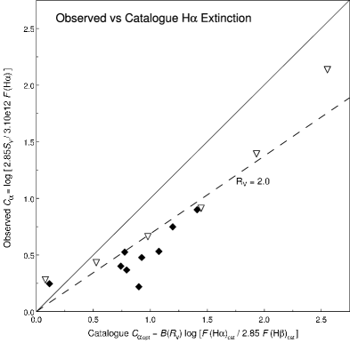
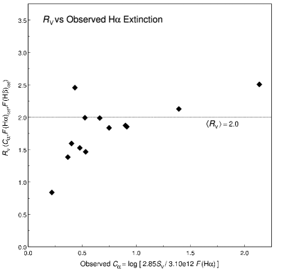
Figure 7: (a) Comparison of observed H$\alpha$ extinction values, $C_{\alpha}=\log\,[2.85\,S_{\nu}\,(6\mathrm{cm})/3.10\times 10^{12}\,F(\mathrm{H}\alpha)]$ and catalogued H$\alpha$ extinction values, $C_{\alpha_{\mathrm{opt}}}=B\,(R_{\mathrm{V}})\log\,[F(\mathrm{H}\alpha)_{\mathrm{cat}}/2.85\,F(\mathrm{H}\beta)_{\mathrm{cat}}]$ where $B\,(3.1)=2.36$, for Bulge subset B objects. Diamonds denote objects observed on the first night, triangles the second. (b) Comparison of $R_{\mathrm{V}}$ (equation 14) and observed H$\alpha$ extinction values. 004.0$-$11.1 (M3-29) and 355.1$-$06.9 (M3-21) are excluded.

5.2 Results

Our observed (equation 7) and catalogue (equation 10) extinction values are listed in columns nine and ten of Table 5. At high brightness temperatures, the optical depth of PNe reduces observed radio emission, so the observed extinction values are likely to be unreliable, as are those calculated from radio fluxes below 10 mJy (indicated in column 13). Therefore Fig. 7 (a) only compares observed and catalogue extinction values for a subset of Bulge objects (hereafter subset B) with 100 mJy $>S_{\nu}>$ 10 mJy and $T_{\mathrm{b}}<10^{3}\mathrm{K}$, where $T_{\mathrm{b}}=70.62S_{5\,\mathrm{GHz}}/{\theta_{\mathrm{line}}}^{2}$ (mJy/″). It can be seen that the values determined from our H$\alpha$ flux and catalogued radio flux tend to be lower than those calculated with $R_{\mathrm{V}}=3.1$ and catalogue H$\alpha$ and H$\beta$ fluxes. Subset B conforms to the Bulge criteria of Bensby & Lundström (2001) with the exception of 004.0$-$11.1 (M3-29) where $b=-11.1\degr$ and 350.9$+$04.4 (H2-1) where $S_{5\,\mathrm{GHz}}=61$ mJy.

Calculated values for $R_{\mathrm{V}}$ (equation 14) are listed in column 11 of Table 5. Fig. 7 (b) compares $R_{\mathrm{V}}$ with observed H$\alpha$ extinction values for subset B. The value of $R_{\mathrm{V}}$ is seen to be highly sensitive to differences between $C_{\alpha}$ and $C_{\alpha_{\mathrm{opt}}}$ with values $>10$ for objects 004.0$-$11.1 (M3-29) and 355.1$-$06.9 (M3-21) not included in the figure for the sake of clarity (regardless of method, calculated extinction values for these two objects are very low with $\Delta F(\mathrm{H}\alpha)=0.1$, suggesting a possible error in the catalogue radio values). Apart from the value for 009.4$-$09.8 (M3-32) and the above two objects, there appears to be a correlation between increasing values of $R_{\mathrm{V}}$ and observed H$\alpha$ extinction.

Because of the sensitivity of $R_{\mathrm{V}}$ to differences between observed and catalogue extinction values, and the uncertainty in these values, a reasonable error $\Delta R_{\mathrm{V}}$ has been calculated with $C_{\alpha}\pm 0.1$ using

$$\Delta R_{\mathrm{V}}=R_{\mathrm{V}}(C_{\alpha}+0.1)-R_{\mathrm{V}}(C_{\alpha}-0.1).$$ (15)

Using $\Delta R_{\mathrm{V}}$ as the error in $R_{\mathrm{V}}$, the mean value $\langle R_{\mathrm{V}}\rangle$ for subset B is found to be 2.0 (indicated on Fig. 7). Values for $\Delta R_{\mathrm{V}}$ are listed in column 12 of Table 5. For subset B a comparison of $R_{\mathrm{V}}$ with catalogue 6 cm radio values shows no evidence of a correlation between low values of $R_{\mathrm{V}}$ and low radio fluxes. In fact, radio flux values would have to increase by a factor $\sim 3$ in order for $\langle R_{\mathrm{V}}\rangle\approx 3.1$.

Fig. 8 compares $R_{\mathrm{V}}$ with Galactic distribution for subset B (again excluding 004.0$-$11.1 and 355.1$-$06.9). For the line of sight towards 351.1$+$04.8, the three objects close together on the sky (H2-1, M1-19 and M2-5) have, within their uncertainties, $\langle R_{\mathrm{V}}\rangle=1.2$. It is worth noting that the two Sagittarius dwarf galaxy objects 004.8$-$22.7 (He2-436) and 006.8$-$19.8 (Wray16-423) have $R_{\mathrm{V}}=3.1$ within their uncertainties.

Objects 352.6$+$00.1 (H1-12) and 352.8$-$00.2 (H1-13) have not been included in subset B because of their very high radio flux and being in the Galactic plane. Caswell & Haynes (1987) identify these positions with H ii regions with $S_{5\,\mathrm{GHz}}$ of 2.1 and 2.8 Jy respectively, giving higher values of $R_{\mathrm{V}}$ (2.4 and 3.5 respectively).

  

Figure 8: Comparison of $R_{\mathrm{V}}$ with Galactic distribution for Bulge subset B objects. Relative $R_{\mathrm{V}}$ is indicated by dot size with $R_{\mathrm{V}}=2.0$ scale indicated at top right. 004.0$-$11.1 (M3-29) and 355.1$-$06.9 (M3-21) are excluded.

Values for $R_{\mathrm{V\,cat}}$ and $\Delta R_{\mathrm{V\,cat}}$ were also calculated using catalogue H$\alpha$ flux values in place of our observed values. The mean catalogue value $\langle R_{\mathrm{V\,cat}}\rangle$ for subset B was found to be 2.2 and for the line of sight towards 351.1$+$04.8 it was 1.4. A comparison of observed and catalogue $R_{\mathrm{V}}$ values shows good agreement for subset B, apart from values for 009.4$-$09.8 (M3-32), 352.1$+$05.1 (M2-8) and 003.6$+$03.1 (M2-14). This suggests that in addition to our newly observed H$\alpha$ flux values, existing catalogue flux values also predict that interstellar extinction toward the Bulge is lower than that corresponding to the standard extinction curve $R_{\mathrm{V}}=3.1$. A comparison of observed and catalogue $S_{\nu}$/H$\alpha$ extinction values also shows good agreement for subset B, apart from values for 352.1$+$05.1 (M2-8) and 003.6$+$03.1 (M2-14), which have differences between observed and catalogued H$\alpha$ flux values, $\Delta F(\mathrm{H}\alpha)$ of 0.4 and 0.8 respectively. Excluding the above three objects from subset B has no effect of the calculated values of $\langle R_{\mathrm{V}}\rangle$ and $\langle R_{\mathrm{V\,cat}}\rangle$. There is no evidence for systematic differences due to time of observation or position in the sky for these three objects.

6 Discussion: Extinction

6.1 Evidence for anomalous extinction

In an optical and UV analysis of Bulge PNe, Walton, Barlow & Clegg (1993) found that $R_{\mathrm{V}}=2.29\pm 0.50$, concluding that the reddening law is steeper towards the Bulge. Stasinska et al. (1992, hereafter STAS) and Tylenda et al. (1992, hereafter TASK) discuss methods for determining the interstellar extinction of Galactic PNe and compare the two most frequently used; the Balmer decrement H$\alpha$/H$\beta$ ratio method and the radio/H$\beta$ flux ratio method. Like all methods, the Balmer decrement method depends on the adopted extinction curve (or mean interstellar extinction law). In addition, it requires good quality optical data acquired by filter photometry, or spectrophotometry that encompasses the full extent of the nebula.

In principle, the radio/H$\beta$ flux ratio method is directly capable of determining the actual value of H$\beta$ extinction, $C_{\beta}$. However, optical thickness of the nebula can lead to an underestimation of $C_{\beta}$. In addition, the predicted H$\beta$ flux depends on adopted electron temperature and He ionization. Blending of He ii Pickering 8 emission with H$\beta$ flux also adds a (very) small error. Interferometric radio data is preferred over single dish measurements because of the problem of confusion with other sources. Zijlstra, Pottasch & Bignell (1989) have noted that their VLA fluxes are systematically lower than the results from single dish observations, due to possible cutting off of emission from fainter, extended regions of PNe. However, as noted previously, for subset B these 6 cm radio fluxes would have to be underestimated by a factor of $\sim 3$ for $\langle R_{\mathrm{V}}\rangle\approx 3.1$. Allowing that radio fluxes below 10 mJy are often underestimated for many faint PN (e.g. Pottasch & Zijlstra, 1994), strong radio sources still have $C_{\mathrm{opt}}$ higher than $C_{\mathrm{rad}}$.

TASK compared the extinction values $C_{\mathrm{rad}}$ and $C_{\mathrm{opt}}$ for Bulge and Disk PNe (their figs. 6 to 11), and showed that, for all PNe, $C_{\mathrm{rad}}$ becomes systematically smaller than $C_{\mathrm{opt}}$ for increasing extinction. They proposed that one of the possible reasons (as mentioned by Cahn, Kaler & Stanghellini, 1992) may lie in the value of $R_{\mathrm{V}}$ adopted in the extinction curve. They estimated that $R_{\mathrm{V}}=2.7$ would bring $C_{\mathrm{opt}}$ to a rough agreement with $C_{\mathrm{rad}}$.

Koppen & Vergely (1998) analysed the optical extinction of 271 Bulge PNe, and found (see their figs. 1 and 2) a mean extinction around $C_{\mathrm{opt}}=2$, and a systematic decrease of the extinction (from 3.5 to 0.5) with increasing Galactic latitude, as well as a genuine scatter about the relation. Both are accounted for by a model of small dust clouds randomly distributed in an exponential disc. They found an extinction $A_{\mathrm{V}}=1.4$ in the plane, and = 27 to the centre, in agreement with far IR-studies (COBE results).

The standard extinction law for the diffuse interstellar medium is based on observations of O and B stars within a few kpc, but these stars must suffer sufficient extinction to allow measurement of their reddening. This selection effect favours denser regions of the interstellar medium in the Solar neighbourhood. For PNe the lines of sight are longer and could cross a more dilute medium while still giving measurable extinction. A lower value of $R_{\mathrm{V}}$ ($<2.5$) could be due to a different size distribution of dust particles (i.e. smaller) in these more dilute regions. For the line of sight toward HD 210121, obscured by the high-latitude cloud DBB 80, Larson et al. (1996, 2000) find $R_{\mathrm{V}}=2.1\pm 0.2$, which they attribute to an abundance of small dust grains.

More recently Udalski (2003) presents results of analysis of photometric data of Bulge fields from the OGLE II microlensing survey (Udalski et al., 2002). He shows $R_{\mathrm{V}}$ in general to be much smaller than that corresponding to the standard extinction curve $R_{\mathrm{V}}=3.1$, and that it varies considerably along different lines of sight. Popowski (2000) has also suggested that interstellar extinction toward the Bulge might be anomalous. Using CCM’s extinction law model, Udalski calculates values for $R_{\mathrm{V}}$ ranging from 1.75 to 2.50 in four small regions of the Bulge. Assumed mean brightness, metallicity distribution, and large differences in the mean distance of red clump giants are all dismissed as unlikely reasons for these highly variable values of $R_{\mathrm{V}}$.

Our results confirm these previous findings, and we find evidence for even lower vales of $R_{\mathrm{V}}$. We believe our flux and extinction determinations to be accurate because: our observed H$\alpha$ fluxes are based on filter photometry; catalogue H$\alpha$ and H$\beta$ flux ratios are normally based on single spectra and are unlikely to suffer from systematic errors (even if the absolute fluxes are in doubt); and although catalogue radio fluxes are less certain, we have used a more reliable subset of Bulge objects ($S_{\nu}>$ 10 mJy and $T_{\mathrm{b}}<10^{3}\mathrm{K}$) for calculating values for $R_{\mathrm{V}}$ and $\Delta R_{\mathrm{V}}$. However, radio fluxes should be remeasured to obtain the most accurate value for $R_{\mathrm{V}}$. Our mean value of $\langle R_{\mathrm{V}}\rangle=2.0$ provides further evidence that most lines of sight towards the Bulge cross a less dense medium containing smaller dust grains. It may be the case that the standard extinction law for the diffuse interstellar medium only applies to the local region within a few kpc of our Sun.

6.2 Extinction and the warm ionized medium

The PNe in our Bulge subset B sample have extinction up to $A_{\mathrm{V}}\approx 5$. The usual conversion between extinction and hydrogen column density, e.g.,

$$N({\rm H})\approx A_{\mathrm{V}}\,2\times\,10^{22}\,\rm cm^{-2}$$ (16)

gives column densities up to $10^{23}\,\rm cm^{-2}$. For a line of sight of 8 kpc, the average density becomes $n_{\rm H}\leq 4\,\rm cm^{-3}$.

Components of the interstellar medium are: Molecular clouds; Diffuse clouds; Warm neutral medium (WNM); Warm ionized medium (WIM); and Hot ionized medium (HIM). The warm neutral medium (WNM) has a typical density of 0.1–10 cm^-3, and scale height around 220 pc. The warm ionized medium (WIM) has a typical density of 0.3–10 cm^-3 in the Galactic plane, with a scale height of 1 kpc (Boulares & Cox, 1990). The HIM has density below 0.01 cm^-3 and a scale height of 3 kpc. The WNM, WIM and HIM account for most of the volume in the Galactic disc. The WNM is absent near the Sun (within 100 pc in most directions): the local volume is filled with a HIM with embedded cold clouds.

Our extinction values of $A_{\mathrm{V}}\leq 5$ mag suggest that the lines of sight do not intercept dense molecular clouds. The density in the HIM is too low to give appreciable extinction even out to the Bulge. The extinction to the Bulge PNe is likely to arise from a mixture of WIM and WNM. The line of sight at higher latitudes leaves the WNM within 2–3 kpc (no Bulge PNe are known within 2 degrees of the plane): the remainder will be mainly within the WIM.

The relation between $R_{\mathrm{V}}$ and $C_{\alpha}$ depicted in Fig. 7 (b) suggests that the lowest $R$ values correspond to the lower density ISM component. A large fraction of the lines of sight fall in WIM-dominated regions above/below the disc. The WNM component is more likely to cause the variable amount of additional extinction. The fact that three PNe located within a degree of each other show very similar – and very low – $R_{\mathrm{V}}$ shows that the low-density structures are similar for line of sights within approximately 100 pc: this provides support for the identification of this component with the WIM. If correct, the distribution of $R_{\mathrm{V}}$ in Fig. 7 (b) suggests that the WIM has $R_{\mathrm{V}}\approx 1.5$, and the WNM $R_{\mathrm{V}}\approx 2.5$. The latter value is close to the lowest local values found by CCM.

The anomalous extinction towards the Bulge therefore suggest that the WIM shows smaller dust grains than found in the WNM or molecular clouds. Possible explanations include dust-grain evolution, and the effects of supernovae. The ISM cycles between high-density and low-density phases. If the dust is slowly destroyed during the low-density phases, the size of the dust grains may measure the time since the last high density phase. The large scale height of the WIM suggests its contents may cycle much slower.

Supernova-driven shocks can also destroy dust grains. Supernovae are more dominant in the inner galaxy (Heiles, 1987): The low-density medium in the inner Galaxy could therefore show systematically smaller dust grains. This would limit the applicability of the standard Galactic extinction curve to quiescent regions of the Galaxy, with steeper curves found in energetic environments.

6.3 Grain sizes

         

Figure 9: Left: A plot, between 0.3 and 1.0 microns, of the absorption, scattering and extinction cross-sections for a Greenberg model with a turnover radius of 0.08 microns, $q=2$, and core radius equal to 0.042 microns. The cross-sections are measured relative to an area of $2.147\times 10^{-16}\,\rm m^{-2}$; Right: Calculated values for $R_{\mathrm{V}}$ for a Greenberg dust model, as function of the turnover radius for the size distribution.

Although different from the locally derived values of $R_{\mathrm{V}}$, it is possible to show that our low values derived above can be reproduced using dust models.

The Greenberg unified dust model (Greenburg & Li, 1996; Li & Greenberg, 1997) is capable of generating a variety of values of $R_{\mathrm{V}}$, which encompass the observational value derived in the present work, by varying the turnover radius, a key parameter of the model.

Li & Greenberg (1997) use a three component model to compute the entire interstellar extinction law: large composite grains, small carbonaceous grains and a population of PAH molecules. In the present work, we consider only the large composite grains, which consist of a silicate core and a refractory organic mantle. Addition of the smaller components would tend to increase ultraviolet extinction relative to that in the visible, and thus drive the model results in the present work to smaller values of $R_{\mathrm{V}}$. The size distribution function used for the composite grains is (Li & Greenberg, 1997)

$$n(a)=n_{0}\exp\left\{-5\left(\frac{a-a_{c}}{a_{m}}\right)^{q}\right\}$$ (17)

where $n(a)$ is the number density of grains of total radius $a$. These composite grains have a silicate core of radius $a_{c}$, and a turnover radius, $a_{m}$. The exponent, $q$, ensures that the distribution of grains falls rapidly for sizes larger than $a_{m}$. In the present work we use values of $q=2$, as in Li & Greenberg (1997), and set $a_{c}=0.042$ $\mu$m which was the radius of infinite cylinders in Li & Greenberg, but spheres in the present work. The value of $a_{m}$ was varied to generate a table of theoretical values of $R_{\mathrm{V}}$. The core material used by Greenburg & Li (1996) was based on values for an amorphous olivine (Dorschner et al., 1995). In the present work we replace the olivine by amorphous forsterite, defined by optical constants (in Scott & Duley, 1996), on the grounds that the olivine contains iron, whilst interstellar silicate is now believed to be dominated by magnesium-rich minerals (see, for example, Kimura et al., 2003). Optical constants for the organic refractory mantle were taken from Greenburg & Li (1996).

Fig. 9 (left panel) shows the optical scattering and absorption coefficients, and the extinction law, for the adopted ‘standard’ model, with one particular value of the turnover radius, $a_{m}=0.08$ $\mu$m. In Fig. 9 (right panel), we plot the value of $R_{\mathrm{V}}$ as a function of the turnover radius, $a_{m}$. The theoretical values shown encompass all values of $R_{\mathrm{V}}$ from the smallest-but-one of the observational figures obtained in the present work, through the rest of the present samples and the more traditional values of $\sim 3.1$ expected for dust in diffuse clouds, to values in excess of $5$, expected for dense, cold, clouds. We note that the key parameter is the amount of grain material found in large grains (with radii larger than $\sim 0.1$ $\mu$m).

We also note that, for any value of $a_{m}$, a smaller value of $R_{\mathrm{V}}$ may be obtained by adding the populations of small carbonaceous grains and PAHs, whilst a larger value is computable by overlaying the composite grains with layers of ices, as is likely in cold clouds. For a comparison of ice-coated and bare grains, see Gray (2001).

7 Conclusions

7.1 Angular diameters

We have calculated angular diameters for 69 PNe by deconvolving the point spread function of field stars from Gaussian FWHM profiles. A correction factor, $\gamma$, was applied to determine the true diameter. $\gamma$ was approximated by a simple analytic function and diameters were calculated using two models: a constant emissivity shell 0.8, $\theta_{\mathrm{shell}}$, and photoionization line emission, $\theta_{\mathrm{line}}$. We present the mean value derived from the two models, $\theta_{\mathrm{mean}}$, as our best estimate. For some objects the low intensity contour plots revealed an elliptical structure that was not always apparent from the FWHM measurements. Axis averaged mean angular diameters of fully resolved objects ranged from $2.8\pm 0.1$ to $12.7\pm 1.2$ arc seconds. 18 H$\alpha$ images were restored with the Richardson-Lucy algorithm and restored diameters tended to be around one arc second smaller below 4 arc seconds.

7.2 Fluxes

The total flux detected through the filters was calculated for 70 PNe. Doppler shifted H$\alpha$, [O iii] (and [N ii]) wavelengths observed at the telescope were computed from radial velocities, and filter transmission coefficients applied to arrive at actual flux densities. For H$\alpha$ and [O iii] there is little evidence of any systematic differences between observed and catalogued flux values. The accuracy of filter response data was considered the most significant source of error and estimated at between $\pm$5 to $\pm$10 per cent.

7.3 Extinction

Observed H$\alpha$ extinction in the direction of the Bulge was determined using the radio to H$\beta$ flux ratio, the expected to observed H$\beta$ flux ratio and the Balmer-line intensity ratio, giving an expression in terms of observed H$\alpha$ flux and catalogue radio flux. Catalogue H$\alpha$ extinction values were also derived from catalogued H$\alpha$ and H$\beta$ flux values in terms of the fundamental extinction law $A(\lambda)/A(V)$ by means of an $R_{\mathrm{V}}$ dependent function. We compared observed and catalogue extinction values for a subset of Bulge objects and found that values determined from observed H$\alpha$ flux and catalogued radio flux tended to be lower than those calculated with $R_{\mathrm{V}}=3.1$ and catalogue H$\alpha$ and H$\beta$ fluxes. A method for determining $R_{\mathrm{V}}$ was derived in terms of observed extinction and catalogued H$\beta$ and H$\alpha$ flux values. We found $R_{\mathrm{V}}$ to be highly sensitive to differences between observed and catalogue extinction values. There also appears to be a correlation between increasing values of both $R_{\mathrm{V}}$ and observed H$\alpha$ extinction, which is in agreement with the findings of STAS discussed above. Estimating a reasonable error in $R_{\mathrm{V}}$, we find observed $\langle R_{\mathrm{V}}\rangle=2.0$, which fits within the range calculated by Udalski and agrees with his conclusion that toward the Bulge interstellar extinction is steeper than $R_{\mathrm{V}}=3.1$. Using catalogue H$\alpha$ and $S_{\nu}$ flux values we find good agreement, with $\langle R_{\mathrm{V\,cat}}\rangle=2.2$. For one small region in our sample we find $\langle R_{\mathrm{V}}\rangle$ as low as 1.2, which suggests that $R_{\mathrm{V}}$ does indeed vary considerably along different lines of sight. We have shown that our values of $R_{\mathrm{V}}$ can be reproduced using dust models with a turnover radius of 0.08 microns. A lower value of $R_{\mathrm{V}}$ may also be obtained by adding the populations of small carbonaceous grains and PAHs.

References

- Acker et al. (1992) Acker A., Marcout J., Ochsenbein F., Stenholm B., Tylenda R., 1992, Strasbourg - ESO catalogue of galactic planetary nebulae, ESO, Garching
- Balick (1987) Balick B., 1987, AJ, 94, 671
- Bedding & Zijlstra (1994) Bedding T. R., Zijlstra A. A., 1994, A&A, 283, 955 (BZ)
- Bensby & Lundström (2001) Bensby T., Lundström, I., 2001, A&A, 374, 599
- Boulares & Cox (1990) Boulares A., Cox D. P., 1990, ApJ, 365, 544
- Cahn, Kaler & Stanghellini (1992) Cahn J. H., Kaler J. B., Stanghellini L., 1992, A&ASS, 94, 399
- Cardelli, Clayton & Mathis (1989) Cardelli J. A., Clayton G. C., Mathis J. S., 1989, ApJ, 345, 245 (CCM)
- Caswell & Haynes (1987) Caswell J. L., Haynes R. F., 1987, A&A, 171, 261
- Dorschner et al. (1995) Dorschner J., Begemann B., Henning T., Jaeger C., Mutschke H., 1995, A&A, 300, 503
- Dudziak et al. (2000) Dudziak G., Péquignot D., Zijlstra A. A., Walsh J. R., 2000, A&A, 363, 717
- Durand et al. (1998) Durand S., Acker A., Zijlstra A. A., 1998, A&ASS, 132, 13
- Gray (2001) Gray M. D., 2001, MNRAS, 324, 57
- Greenburg & Li (1996) Greenberg J. M., Li A., 1996, A&A, 309, 258
- Hamuy et al. (1994) Hamuy M., Suntzeff N. B., Heathcote S. R., Walker A. R., Gigoux P., Phillips M. M., 1994, PASP, 106, 566
- Heiles (1987) Heiles C., 1987, ApJ, 315, 555
- Kimura et al. (2003) Kimura H., Mann I., Jessberger E. K., 2003, ApJ, 583, 314
- Koppen & Vergely (1998) Koppen J., Vergely J.-L., 1998, MNRAS, 299, 567
- Larson et al. (1996) Larson K. A., Whittet D. C. B., Hough J. H., 1996, ApJ, 472, 755
- Larson et al. (2000) Larson K. A., Wolff M. J., Roberge W. G., Whittet D. C. B., He L., 2000, ApJ, 532, 1021
- Li & Greenberg (1997) Li A., Greenberg J. M., 1997, A&A, 323, 566
- Lucy (1974) Lucy L. B., 1974, AJ, 79, 745
- Minniti (1996) Minniti D., 1996, ApJ, 459, 175
- Popowski (2000) Popowski P., 2000, ApJ (Letters), 528, L9
- Pottasch (1984) Pottasch S. R., 1984, Planetary Nebulae, Reidel, Dordrecht, p. 41, 92, 95 (SP)
- Pottasch & Zijlstra (1994) Pottasch S. R. & Zijlstra A. A., 1994, A&A, 289, 261
- Reid (1993) Reid M., 1993, ARA&A, 31, 345
- Richardson (1972) Richardson W. H., 1972, Jou. Opt. Soc. Am., 62, 55
- Scott & Duley (1996) Scott A., Duley W. W., 1996, ApJS, 105, 401
- Stasinska et al. (1992) Stasinska G., Tylenda R., Acker A., Stenholm B., 1992, A&A, 266, 486 (STAS)
- Tylenda et al. (1992) Tylenda R., Acker A., Stenholm B., Koeppen J., 1992, A&ASS, 95, 337 (TASK)
- Tylenda et al. (2003) Tylenda R., Siódmiak N., Górny S. K., Corradi R. L. M., Schwarz H. E., 2003, A&A, 405, 627
- Udalski (2003) Udalski A., 2003, ApJ, 590, 284
- Udalski et al. (2002) Udalski A., Szymanski M., Kubiak M., Pietrzynski G., Soszynski I., Wozniak P., Zebrun K., Szewczyk O., Wyrzykowsk L., 2002, Acta Astron., 52, 217
- van Hoof (2000) van Hoof P. A. M., 2000, MNRAS, 314, 99 (VH)
- Walton, Barlow & Clegg (1993) Walton N. A., Barlow M. J., Clegg R. E. S., 1993, IAU Symp. 153: Galactic Bulges, 153, 337
- Zijlstra, Pottasch & Bignell (1989) Zijlstra A. A., Pottasch S. R., Bignell C., 1989, A&ASS, 79, 329