[astro-ph/0407175] The generalized Roche model

1 Introduction

The classic Roche model describes the equilibrium figure of the rotating massless liquid (gas) envelope in the gravitational field of the point mass [1,2]. It is widely used in investigation of the structure of the rotating star with a large enough value of the effective polytropic index, when there is a strong concentration of a matter to the star’s center and one may ignore the self-gravitation of the outer layers of the star as compared with the gravitation of the star’s central core. In the opposite limit of rotation of the incompressible liquid with constant density, the Maclarain ellipsoidal models are used [1,2].
The next natural generalization of the classic Roche model would be the taking into account the effects of the non-spherical gravitational field of the star’s core, still neglecting the self-gravitation of the (uniformly) rotating envelope. In this note we consider one of the possible approaches to the problem [3].

2 Basic Equations

2.1 Gravitational potential of two fixed centers

We use a common set of rectangular coordinates: $x$ - and $y$ -axes are in the equatorial plane, $z$ -axis coincides with the axis of rotation, the center of coordinate system $(0,0,0)$ coincides with the star’s center.
Let two fixed points with equal masses $m_{1}=m_{2}=M/2$ be placed at $z$ -axis such that coordinates of the ’ $centers$ ’ are $\left(0,0,z_{1}\right)$ and $\left(0,0,z_{2}\right)$ , where $z_{1}=i\,c,\;z_{2}=-i\,c,\;i^{2}=-1$ .
Then gravitational potential has the axis of symmetry, $z$ -axis, (axis of rotation), and the plane of symmetry, $z=0$ plane, (equatorial plane). For our problem it is sufficient to consider the gravitational potential in $\left(x,z\right)$ -plane (meridional plane)

V(x,z)=\frac{G\,M}{2}\,(\frac{1}{r_{1}}+\frac{1}{r_{2}}),

(1)

r_{1}^{2}=x^{2}+(z-i\,c)^{2},\ r_{2}^{2}=x^{2}+(z+i\,c)^{2},

(2)

where $G$ is the gravitational constant, $M$ is the star mass, $r_{1}$ and $r_{2}$ are distances from the point $(x,z)$ to fixed centers, $c$ is the (positive) constant of the two fixed centers problem describing the deviation of the gravitational potential from the spherical symmetry. Hereafter all formulas reduce to the classical Roche model case at the limit $c\rightarrow 0$ .

2.2 Reality of gravitational potential

Gravitational potential (1,2) is of course real (while $r_{1}$ and $r_{2}$ not), and in order to show it we introduce, instead of rectangular coordinates $\left(x,z\right)$ , two real positive variables $\lambda$ and $\mu$ defined by the following relations:

r_{1}=c\,(\lambda-i\,\mu),\ \ r_{2}=c\,(\lambda+i\,\mu),

(3)

\lambda=\frac{r_{1}+r_{2}}{2\ c},\ \ \mu=\frac{r_{2}-r_{1}}{2\ c},

(4)

x^{2}=c^{2}\,(1+\lambda^{2})\,(1-\mu^{2}),\ \ z^{2}=c^{2}\ \lambda^{2}\ \mu^{2}.

(5)

From Equations (1)–(5) we get

V(\lambda,\mu)=\frac{G\,M}{c}\frac{\lambda}{\lambda^{2}+\mu^{2}},

(6)

which is real, QED.
Note that $(\lambda,\mu)$ coordinates are sometimes called (oblate or prolate) confocal ellipsoidal coordinates, or simply ellipsoidal coordinates, or even elliptic coordinates, see e.g. [4,5]. Also notes that authors use different notations for these coordinates. At $(x,z)-$ plane, the curves $\lambda$ =const are confocal ellipses with focuses at points $(x=0,\,z=+c)$ and $(x=0,\,z=-c)$ while the curves $\mu$ =const being normal to curves $\lambda$ =const are hyperbolas.

2.3 Total potential

Potential of rotational forces is

U(x)=\frac{1}{2}\,\omega^{2}\,x^{2},

(7)

where $\omega=$ const is the angular velocity of rotation. The total potential is a sum of gravitational and rotational potentials

\Phi(x,z)=V(x,z)+U(x).

(8)

Again we note that the total potential has an axis and a plane of symmetry though we consider only $(x,z)-$ plane (meridian plane) and more specifically, first quadrant of $(x,z)-$ plane with positive $x$ and $z$ .

3 Arbitrary rotation in the classic Roche problem

The form of the equilibrium rotating massless envelope in the CRM depends on degree of rotation: non-rotating envelope has spherical form, for slow rotation the figure is spheroid (figure of rotation with meridional section as ellipse), for larger rotation the figure is more and more oblate (and not spheroid), until the critical figure is attained, when at the equator of the figure, the centrifugal force is equal to gravitational force. Note that critical figure has a cusp at equator. For arbitrary value of angular velocity $\omega$ the total potential at the equator (where $r=x=a$ ) is

\Phi_{c}=\frac{GM}{a}+\frac{1}{2}\omega^{2}a^{2}.

(9)

The equilibrium figure is defined by the equation

\frac{GM}{r}+\frac{1}{2}\omega^{2}x^{2}=\frac{GM}{a}+\frac{1}{2}\omega^{2}a^{2},

(10)

from here we find the polar radius ( $x=0,r=z=b$ )

\frac{GM}{b}=\frac{GM}{a}+\frac{1}{2}\omega^{2}a^{2};

(11)

for the ellipticity $f=1-a/b$ of the equilibrium figure and centrifugal-to-gravitational force ratio at equator $m=\omega^{2}a/(GM/a^{2})$ we have the general expression

\frac{f}{m}=\frac{1}{2+m}.

(12)

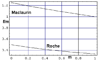
We see that, in the CRM, the ratio $f/m$ varies from maximal value of $1/2$ (for slow rotation, $m\ll 1$ ), to minimal value of $1/3$ (for maximal rotation, $m=1$ ). Note that sometimes authors use in $m$ centrifugal force at equator and mean gravitational force which is OK in the first approximation in $\omega^{2}$ but has no much sense at strong rotation.
For comparison, for Maclaurin spheroids, the $f/m$ ratio varies from 5/4 to 1 for $m$ varying from 0 to 1, see Fig. 1.

Refer to caption — Figure 1: Ellipticity of rotating fluid in Maclaurin and Roche models: abscissae is $m$ , centrifugal-to-gravitational force ratio at equator of the figure, ordinate is $f/m$ , where $f=1-b/a$ is ellipticity, and $a$ and $b$ are equatorial and polar radii.

4 Critical figure in the GRM:
Polar and equatorial radii

Let us write down the gravitational potential (1,2) and the total potential (8) on $x$ -axis, where $z=0,\ \ r_{1}=r_{2}=\sqrt{x^{2}-c^{2}},\ \ x>c>0$

V(x)=\frac{G\,M}{\sqrt{x^{2}-c^{2}}},\ \ \Phi(x)=V(x)+U(x).

(13)

The critical surface is defined by a condition of equality of centrifugal and gravitational forces, - $\partial V(x)/\partial x=\partial U(x)/\partial x$ , or by a minimum of the total potential, $\partial\Phi(x)/\partial x=0$ , at some $x=a$ . This gives the equation for the equatorial radius $a$ :

\frac{G\,M}{\left(a^{2}-c^{2}\right)^{3/2}}=\omega^{2}.

(14)

4.1 Equatorial radius

From Equation (14), the equatorial radius of the critical surface is

a=\sqrt{\left(\frac{G\,M}{\omega^{2}}\right)^{2/3}+c^{2}}.

(15)

We note that the equatorial radius of the rotating star with the same mass $M$ and angular velocity $\omega$ is larger than the equatorial radius $a_{0}$ in the classical Roche model

a_{0}=\left(\frac{G\,M}{\omega^{2}}\right)^{1/3}.

(16)

4.2 Polar radius

From equations (7)-(15), we write the total potential at the critical surface as

\Phi_{0}=\frac{G\,M}{2}\frac{3\,a^{2}-2\,c^{2}}{\sqrt{\left(a^{2}-c^{2}\right)^{3}}}=\frac{\omega^{2}}{2}\left(3\,a^{2}-2\,c^{2}\right).

(17)

On rotational, $z$ , axis, where $x=0,\ \ r_{1}=z-c\,i,\ \ r_{2}=z+c\,i,\ \ z>c>0$ , we have only the gravitational potential (because the rotational potential vanishes at $z$ -axis)

V(z)=G\ M\frac{z}{z^{2}+c^{2}}.

(18)

The polar radius of the critical figure is defined by the condition $\Phi_{0}=V(z)$ , and from equations (17) and (18), we find the polar radius of the critical figure

b=A+\sqrt{A^{2}-c^{2}},\ \ A=\frac{(a^{2}-c^{2})^{3/2}}{3a^{2}-2c^{2}}.

(19)

Note that we choose plus sign before radical in (19) such that $b>c$ , also we note that usually the value of the constant $c$ of the two fixed centers model is much less than dimensions of the figure (star or planet).
From (14) we have unequality for the equatorial radius $a>c$ , additionally from condition $b>c$ , ( $A>c$ ), and (19), we get the lower boundary for the equatorial radius

a>a_{1},\ \ \frac{a_{1}}{c}=\sqrt{4+{\left(\frac{73-\sqrt{5}}{2}\right)}^{1/3}+{\left(\frac{73+\sqrt{5}}{2}\right)}^{1/3}}.

(20)

Numerically, $a_{1}/c=3.26092$ [5].

4.3 Two limits

At limit of small deviations from the classical Roche model, $a\gg c$ , $b\gg c$ , we have for equatorial, $a$ , and polar, $b$ , radii and their ratio $b/a$

a=a_{0}\,\left(1+{\frac{1}{2}}\,{\frac{c^{2}}{a_{0}^{2}}}\right),\ \ a_{0}=\left({\frac{G\,M}{\omega^{2}}}\right)^{1/3},

(21)

b=b_{0}\,\left(1-{\frac{31}{12}}\,{\frac{c^{2}}{a_{0}^{2}}}\right),\ \ b_{0}={\frac{2}{3}}\,a_{0},

(22)

{\frac{b}{a}}=\frac{2}{3}-\frac{37}{18}\,\left(\frac{c}{a_{0}}\right)^{2}-\frac{1025}{216}\,\left(\frac{c}{a_{0}}\right)^{4}.

(23)

We note that comparing with CRM, in GRM, the equatorial radius $a$ is larger, while the polar radius $b$ and the polar-to-equatorial radius ratio $b/a$ is less. That is in GRM, the critical figure of rotating envelope is more flatten (oblate).
In another limit, at the equatorial radius $a$ close to $a_{1}$ we have

\frac{a}{c}=\frac{a_{1}}{c}+\delta,\ \ 0<\delta\leq\frac{a_{1}}{c};

(24)

\frac{b}{c}=1+\left[\frac{6a_{1}^{3}c\delta}{(a_{1}^{2}-c^{2})(3a_{1}^{2}-2c^{2})}\right]^{1/2};

(25)

\frac{b}{a}=\frac{c}{a_{1}}\left(1-\frac{c}{a_{1}}\delta+[1+\frac{6a_{1}^{3}\delta c}{(a_{1}^{2}-c^{2})(3a_{1}^{2}-2c^{2})}]^{1/2}\right).

(26)

At $\delta=0,a=a_{1}$ ,

{b\over a}=\sqrt{1-{\left(\frac{2}{5\,\left(5+{\sqrt{5}}\right)}\right)}^{\frac{1}{3}}-\frac{1}{5}{\left(\frac{2}{5\,\left(5+{\sqrt{5}}\right)}\right)}^{-\frac{1}{3}}}.

(27)

5 Isopotentials in GRM

In general form the equation for critical figure can be written down using variables $\lambda$ and $\mu$

\frac{GM}{c}\frac{\lambda}{\lambda^{2}+\mu^{2}}+\frac{1}{2}\omega^{2}c^{2}(1+\lambda^{2})(1-\mu^{2})=\Phi_{0},

(28)

where $\Phi_{0}$ and $a$ are given in (17) and (15).
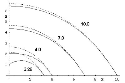
From (17) we have quadratic equation for $\mu^{2}$ as function of $\lambda$ . Further, in variables $x,z$ using (5) we get parametric equation of the complex from (with $\lambda$ as parameter). In result, we present the Fig. 2 the equilibrium critical figures for several values of the equatorial radius $a/c$ . With decreasing $a$ (this corresponding to increasing $\omega$ or increasing $c$ , increasing flatteness of the gravitational field) the deviation of the GRM critical figures from CRM increases and for small values of $a$ the figures become even concave while CRM figures are always convex.

6 Concave figure

Let us find the value $a=a_{2}$ when the equilibrium figure becomes concave first. Expanding (1,2) in the series at small $x\ll 1$ and using (7,8,17), and requiring $dz/dx=0\mbox{ at }x=0$ we have the algebraic equation of the 7th order for $y\equiv a_{2}/c$

144-1512\,y+6408\,y^{2}-14184\,y^{3}+17475\,y^{4}-11553\,y^{5}+3397\,y^{6}-171\,y^{7}=0;

(29)

similarly for corresponding polar radius $b_{2}$ we have again algebraic equations of the same order ( $t\equiv b_{2}/c$ )

81+584\,t+1278\,t^{2}+1500\,t^{3}+882\,t^{4}+195\,t^{5}-45\,t^{6}-19\,t^{7}=0.

(30)

Numerically, we get $a_{2}/c=4.00358,\,b_{2}/c=2.0376,$ and $b_{2}/a_{2}=0.508945.$
At $a>a_{2}$ the critical figures in GRM are convex, at $a<a_{2}$ the critical figures (and also inner isopotentials near the external surface!) are concave.

7 Post-classical approximation

The analysis is more easy in the limit $x\gg c,$ $z\gg c$

(more exactly, $r=(x^{2}+z^{2})^{1/2}\gg c$ ). The gravitational potential up to terms proportional to $c^{2}/r^{2}$ is

V(r,z)=\frac{GM}{r}\left[1+\frac{1}{2}\frac{c^{2}}{r^{2}}-\frac{3}{2}\frac{c^{2}}{r^{2}}\frac{z^{2}}{r^{2}}\right].

(31)

Isopotentials $V(r,z)=V_{c}$ corresponding to (31) are ellipses with larger semi-axis $a$ along $x$ -axis and minor semi-axis $b$ along $z$ -axis

a=r_{0}(1+\frac{1}{2}\frac{c^{2}}{r_{0}^{2}}),\ b=r_{0}(1-\frac{c^{2}}{r_{0}^{2}}),\ r_{0}=\frac{GM}{V_{c}}.

(32)

At $c=0$ we have the equilibrium figure of the CRM

r=\frac{G\ M}{\Phi_{c}-\frac{1}{2}\omega^{2}x^{2}},

(33)

or

r_{0}(x)=\frac{2a}{3-x^{2}/a^{2}},\,\,0\leq x\leq a,\,\,a\geq r_{0}\geq b.

(34)

If $\Phi_{c}>>\frac{1}{2}\omega^{2}x^{2}$ (slow rotation), the equilibrium figure is ellipse

r=\frac{G\ M}{\Phi_{c}}(1+\frac{1}{2}\frac{\omega^{2}x^{2}}{\Phi_{c}})

(35)

with larger semi-axes along the $x$ -axis (equatorial radius) and minor semi-axis along the $z$ -axis (polar radius).
Taking into account terms up to $c^{2}/a_{0}^{2}$ critical figure is

r(x)=r_{0}(x)(1+\beta c^{2}/a_{0}^{2}),\,0\leq x\leq a,\,b\leq r\leq a,

(36)

\beta=-\frac{1}{2t}+\frac{9}{2}t^{4}-3t^{5}-t^{2},\,t\equiv a_{0}/r_{0},

(37)

where $r_{0}(x),\,a_{0},a,\,\mbox{and }b$ are given in Eqs (21-23, 34).
Using (36,37) we may calculate the volume of the critical figure

W=4\,\pi\,\int_{0}^{a}\,z(x)\,x\,dx,\,\,z=\sqrt{r^{2}-x^{2}}.

(38)

In (38) both the integrand $z(x)$ and the upper limit $a$ can be expand in the series up to terms $c^{2}/a_{0}^{2}$

W=4\,\pi\,\left[\int_{0}^{a_{0}}\,z_{0}(x)\,x\,dx,\,+z(a_{0})\cdot a_{0}\cdot(a-a_{0})+\int_{0}^{a}\,z_{1}(x)\,x\,dx\right],

(39)

z_{0}^{2}=r_{0}^{2}-x^{2},\,z=z_{0}+z_{1}\,c^{2}/a_{0}^{2},\,z_{1}=\beta r_{0}^{2}/z_{0}.

Here the first term in W is the volume of critical figure in CRM, second term is proportional to $c^{3}/a_{0}^{3}$ and may me omitted, and third term is proportional to $c^{2}/a_{0}^{2}$ .
Both integrals can be expressed in terms of elementary functions, and we have

\int_{0}^{a_{0}}\,z_{0}(x)\,x\,dx=a_{0}^{3}\int_{0}^{1}\frac{1-x^{2}}{3-x^{2}}(4-x^{2})^{1/2}\ x\ dx=\sqrt{3}-\frac{4}{3}+\ln\left(6-3\sqrt{3}\right),

(40)

\int_{0}^{a_{0}}z_{1}(x)\ x\ dx=\frac{16-27\,{\sqrt{3}}}{210}a_{0}^{3}(c^{2}/a_{0}^{2}).

(41)

The volume of the critical figure is

W=4\,\pi\,a_{0}^{3}\,\left[0.180372-0.146502(c^{2}/a_{0}^{2})\right].

(42)

By introducing the mean density of the critical figure $\overline{\varrho}=M/W$ , we have in the post-classical approximation for parameter widely used in the theory of rotating configurations

{w^{2}\over 2\pi G\overline{\varrho}}={W\over 2\pi a_{0}^{3}}=0.360744-0.293003\,c^{2}/a_{0}^{2}.

(43)

8 Conclusion

We obtained all parameters of rotating configuration in the Roche model taking into account the effects of (small) non-sphericity of the gravitational field of the central body. As a rule any modification of the classical models leads at best to ugly non-elegant analytical or even pure numerical results.
And Roche models are of the best examples of those classical models idealized and elegant both in set up and results.

9 References

1. Kopal Z. Figures of Equilibrium of Celestial Bodies. Madison: Univ. of Wisconsin Press, 1960.
2. Tassoul J-T. Theory of rotating stars. New Jersey: Princeton Univ. Press, 1978.
3. Z.F. Seidov, 1981DoAze..37…18S; 1982DoAze..38…30S
4. Abramowitz, M. and Stegun, I. A. (Eds). ”Definition of Elliptical Coordinates.” §21.1 in Handbook of Mathematical Functions with Formulas, Graphs, and Mathematical Tables, 9th printing. New York: Dover, p. 752, 1972. The book is available also in: http://jove.prohosting.com/ skripty/
5. E. Wassermann, http://mathworld.wolfram.com/ConfocalEllipsoidalCoordinates.html

The generalized Roche model

Abstract