On the evolution of star forming galaxies

Abstract

The evolution in the comoving space density of the global average galaxy star formation rate (SFR) out to a redshift around unity is well established. Beyond $z\approx 1$ there is growing evidence that this evolution is flat or even increasing, contrary to early indications of a turnover. Some recent analyses of $z\approx 6$ photometric dropouts are suggestive of a decline from $z=3$ to $z\approx 6$, but there is still very little constraint on the extent of dust obscuration at such high redshifts. In less than a decade, numerous measurements of galaxy SFR density spanning $z=0$ to as high as $z\approx 6$ have rapidly broadened our understanding of galaxy evolution, and a summary of existing SFR density measurements is presented here. This global star formation history compilation is found to be consistent to within factors of about three over essentially the entire range $0<z\lesssim 6$, and it can be used to constrain the evolution of the luminosity function (LF) for star forming (SF) galaxies. The LF evolution for SF galaxies has been previously explored using optical source counts, as well as radio source counts at 1.4 GHz, and a well-known degeneracy between luminosity evolution ($L\propto(1+z)^{Q}$) and density evolution ($\phi\propto(1+z)^{P}$) is found. Combining the constraints from the global SFR density evolution with those from the 1.4 GHz radio source counts at sub-millijansky levels allows this degeneracy to be broken, and a best fitting evolutionary form to be established. The preferred evolution in a $H_{0}=70,\Omega_{M}=0.3,\Omega_{\Lambda}=0.7$ cosmology from these combined constraints is $Q=2.70\pm 0.60$, $P=0.15\pm 0.60$.

1 Introduction

The increase by an order of magnitude in the global comoving space density of galaxy star formation rate (SFR) from $z=0$ to $z\approx 1$ has been well established by numerous measurements in recent years (e.g., Wilson et al., 2002; Haarsma et al., 2000; Flores et al, 1999; Cowie et al., 1999; Hogg et al., 1998; Hammer et al., 1997; Lilly et al., 1996, see also the list of references in Tables 2 and 4). A large body of data has now been collected to measure this evolution, and the shape of the star formation (SF) history at higher redshifts (now approaching $z\approx 6$). As will be seen, within measurement uncertainties and the limitations of the various surveys used, this large, heterogeneous dataset is highly consistent over the entire redshift range $0<z\lesssim 6$, and constrains the SFR density to within a factor of about three at most redshifts.

With such a wealth of measurements now available, the evolution of the global galaxy SFR density can be used as a robust constraint on various simulations and semianalytic models of galaxy evolution. This is already being pursued by many authors (e.g., Somerville et al., 2001; Pei et al., 1999), and tantalising indications about the details of galaxy evolution are suggested as a result (such as collisionally induced star formation being favoured as the dominant mode of galaxy evolution, as opposed to steady ongoing star formation, Somerville et al., 2001). The richness of the available measurements offers a very strong constraint that must be met by such models, but full advantage has not yet been taken of this important resource.

To illustrate this point, a compilation drawn from the literature of SFR density measurements as a function of redshift is presented here, and constraints on the evolving luminosity function of star forming galaxies are derived. Together with constraints from radio source counts, the SF history data allow the degeneracy between rates of luminosity and density evolution to be broken, and a robust constraint on both is derived.

The details of the measurements from the literature are presented in § 2, and evolving luminosity functions for star forming galaxies are presented in the context of the SF history diagram in § 3. In § 4 the SF history compilation is used in conjunction with the radio source counts to constrain the form for the evolving LF. The results are discussed in § 5, and conclusions summarised in § 6. A flat Lambda cosmology is assumed throughout, as indicated by numerous recent measurements, with $H_{0}=70\,$km s^-1 Mpc^-1, $\Omega_{M}=0.3$, $\Omega_{\Lambda}=0.7$ (e.g., Spergel et al., 2003).

2 The measurements

Measurements of galaxy SFR density have been compiled from the literature, converted to a common cosmology and SFR calibration, and corrected for dust obscuration, where necessary, in a common fashion. This is necessary in order to consistently compare measurements made at different wavelengths. The star formation calibrations chosen are presented in Table 1, all assuming a Salpeter (1955) initial mass function (IMF) and mass range $0.1<M<100\,M_{\odot}$. The H$\alpha$, UV and far infrared (FIR) calibrations adopted are those from Kennicutt (1998). The 1.4 GHz SFR calibration chosen is that of Bell (2003), derived to be consistent with the FIR calibration from Kennicutt (1998). This calibration gives SFRs lower by about a factor of two than the calibration of Condon (1992) for $\log(L_{1.4}/{\rm W\,Hz}^{-1})\gtrsim 21.8$. As luminosity decreases the SFRs approach those of Condon (1992), and become higher for luminosities below $\log(L_{1.4}/{\rm W\,Hz}^{-1})\lesssim 20.5$.

2.1 Cosmology conversion

The conversion from the originally chosen cosmology to that assumed here is as follows. Since in a flat universe comoving volume is proportional to comoving distance cubed, $V_{c}\propto D_{c}^{3}$, the comoving volume between redshifts $z-\Delta z$ and $z+\Delta z$, $V_{c}(z,\Delta z)\propto D_{c}^{3}(z+\Delta z)-D_{c}^{3}(z-\Delta z)$. Since luminosity is proportional to comoving distance squared, $L\propto D_{c}^{2}$, then the SFR density for a given redshift range, (assuming that all galaxies lie at the central redshift),

$$\dot{\rho}_{*}\propto\frac{L(z)}{V_{c}(z,\Delta z)}\propto\frac{D_{c}^{2}(z)}{D_{c}^{3}(z+\Delta z)-D_{c}^{3}(z-\Delta z)}.$$ (1)

So, in order to convert from one cosmology to another, this expression is evaluated for both cosmologies at the appropriate redshift and the ratio used as the conversion factor. This is similarly described by Ascasibar et al. (2002), and an equivalent form used by Hogg (2002).

In the case of converting luminosity functions (LFs), the conversion of the luminosity and volume components need to be done separately. When applying a luminosity-dependent obscuration correction, as described below, the LF being used must first be corrected for the cosmology to ensure that the obscuration corrections applied correspond to the correct luminosities in the final cosmology. To convert the LF, the characteristic luminosity and the volume normalisation factors ($L^{*}$ and $\phi^{*}$ in the Schechter (1976) or Saunders et al. (1990) parameterisations) are converted. This is done in a similar fashion to that described above, using the proportionalities already given.

This procedure for converting cosmologies, with the coarse assumption that all galaxies lie at the central redshift, is only approximate. The expected uncertainties introduced by this assumption, though, even in the case of the measurements spanning the largest redshift ranges, are at most of the order of $10\%$, which is small compared to the factors of two to three by which the actual measurements may differ from each other, as seen below.

2.2 Obscuration corrections

Obscuration by dust is well known to affect measurements of galaxy luminosity at UV and optical wavelengths. Correcting for this effect is not always straightforward, however, since measurements of an obscuration sensitive parameter, such as the Balmer decrement or UV spectral slope, are not always easy to obtain. It has become a standard procedure to make an approximate obscuration correction by assuming an average level of expected obscuration (such as $A_{V}=1\,$mag) and uniformly correcting all objects. This procedure has the advantage that it is straightforward to apply either to a luminosity function or a luminosity density, being simply a scaling factor. Recently, though, it has been shown that galaxies with high luminosities or SFRs tend, on average, to suffer greater obscuration than faint or low SFR systems (Hopkins et al. 2001a; Sullivan et al. 2001; Pérez-González et al. 2003; Afonso et al. 2003; Hopkins et al. 2003c; but see also Buat et al. 2002). Correcting for such a luminosity-dependent (or SFR-dependent) effect is not as straightforward as for a common obscuration, though, since a knowledge of the full LF is necessary. It is further complicated by the fact that the specific relation describing the luminosity-dependent effect is strongly dependent on the selection criteria of the sample being investigated (Afonso et al., 2003; Hopkins et al., 2003c).

These issues are not insurmountable, however, and both a common obscuration and a luminosity-dependent obscuration are explored below. In some cases actual measurements of the obscuration (such as the Balmer decrement) have already been used by the original authors, with obscuration curves consistent with those assumed below, to correct the LFs or the SFR density estimate. These results are always used in favour of invoking less reliable average corrections. It must also be emphasised that although different average obscurations are assumed below for the common obscuration correction, depending on the wavelength used to select the sample being corrected, these are not necessarily inconsistent. They are based on observed average obscurations for similarly selected samples in the literature. Some issues regarding the use of average obscuration corrections are discussed further below, but it should be clear that for surveys that detect only relatively low obscuration systems, for example, a relatively small average obscuration correction is appropriate. The corresponding LF derived from such a sample is then used (by fitting a Schechter function, for example) to infer the details of brighter but more heavily obscured systems that fall below the detection threshold, as well as systems below the survey limit that are fainter and possibly less obscured.

In all obscuration corrections used herein for emission line SFR measurements (H$\alpha$, H$\beta$, [Oii]) the galactic obscuration curve from Cardelli et al. (1989) is used. For continuum measurements (primarily UV wavelengths from 1500 Å to 2800 Å) the starburst obscuration curve from Calzetti et al. (2000) is used (see also Calzetti, 2001). When applying a common obscuration correction, $A_{\rm H\alpha}=1.0\,$mag is assumed for emission line measurements, often found as the average obscuration to H$\alpha$ emission in samples of local galaxies (e.g., Kennicutt, 1992; Hopkins et al., 2003c). Similarly, for UV-selected samples a typical obscuration is found to be $A_{V}=1.0\,$mag (e.g., Sullivan et al., 2000; Tresse et al., 1996), although this value is based on galactic obscuration curves rather than the starburst curves from Calzetti assumed here. To convert this to the appropriate $A_{V}$ for the Calzetti curve, the mean Balmer decrement corresponding to this value is first inferred. The analysis of Sullivan et al. (2000) is used as a reference here, and those authors base their obscuration corrections on the Seaton (1979) galactic obscuration curve. Since $R=A_{V}/E(B-V)$ and $R=3.2$ is assumed, the mean value of $A_{V}=1.0$ (from Sullivan et al., 2000), gives $E(B-V)=0.313$. But $E(B-V)$ also depends on the choice of obscuration curve,

$$E(B-V)=\frac{\log[(f({\rm H\alpha})/f({\rm H\beta}))/2.86]}{0.4(k({\rm H\beta})-k({\rm H\alpha}))}.$$ (2)

(Calzetti et al., 1996). Here $f({\rm H\alpha})/f({\rm H\beta})$ is the Balmer decrement, and $k({\rm H\beta})-k({\rm H\alpha})$ is the difference between the values of the obscuration curve at the wavelengths of H$\beta$ and H$\alpha$. The latter quantity is 1.19 for the Seaton (1979) curve, and gives a Balmer decrement of $4.03$ corresponding to the mean $A_{V}=1$. For the Calzetti et al. (2000) curve, $k({\rm H\beta})-k({\rm H\alpha})=1.27$, and this Balmer decrement gives $E(B-V)_{\rm gas}=0.293$, similar to the above value. Indeed, $A_{V\rm gas}=k(V)E(B-V)_{\rm gas}=1.19$ (with $k(V)=4.05$), a little higher than the 1 mag from the galactic curve. To correct the stellar continuum the relation $E(B-V)_{\rm star}=0.44E(B-V)_{\rm gas}$ is used (Calzetti et al., 2000). The subscript notation “gas” and “star” refer to nebular and stellar continuum obscuration respectively. Finally, $A_{V\rm star}=0.44k(V)E(B-V)_{\rm gas}=0.52$. Note that in Equation 2 it is necessary to use $k(\lambda)$ appropriate for nebular obscuration (Equation 4 of Calzetti et al., 2000). Hence, $A_{V}=1.0$ for the Seaton (1979) curve becomes $A_{V\rm star}=0.52$ for the Calzetti (2001) curve. It would simplify comparisons such as this to have obscuration sensitive quantities presented as observables, such as Balmer decrement or UV spectral slope. These should be elementary to provide in addition to derived values dependent on the chosen obscuration curve, like $A_{V}$ and $E(B-V)$.

To summarise, when a common obscuration correction is performed below, emission line measurements are corrected using $A_{\rm H\alpha}=1.0$ and the Cardelli et al. (1989) galactic obscuration curve, and continuum UV measurements are corrected using $A_{V\rm star}=0.52$ and the Calzetti et al. (2000) starburst obscuration curve.

It is interesting to note that an obscuration at the wavelength of H$\alpha$ of $A_{H\alpha}=1.0\,$mag corresponds to $A_{V}=1.22$, using the galactic obscuration curve of Cardelli et al. (1989), or $A_{V}=1.29$ using the curve of Seaton (1979), compared to $A_{V}\approx 1.0$ (using galactic obscuration curves) found for UV selected samples. This observation is consistent with the expected result that the average obscuration of galaxies selected at redder wavelengths (around H$\alpha$) can be greater than those selected at UV wavelengths where the more heavily obscured systems will not enter the sample. This effect is seen quite strikingly in the radio-selected sample of star forming galaxies analysed by Afonso et al. (2003) who find systematically higher median obscurations at all luminosities than in the optically selected sample explored by Hopkins et al. (2003c).

The analysis of Massarotti et al. (2001), in addition, emphasises the important result that making obscuration corrections based on an average observed $A_{V}$ or $E(B-V)$ will result in an underestimate of the true measurement. They explain that the effective mean obscuration is larger than the mean of the observed obscurations. This implies that the SFR densities obtained using the common obscuration corrections above will be underestimates of the true SFR densities.

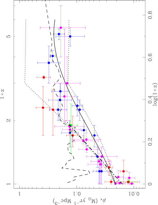
Figure 2: As for Figure 1, with a luminosity-dependent obscuration correction. Symbols and lines as in previous Figure. The least squares fit to the $z<1$ data points (dot-dashed line) in this Figure is $\log(\dot{\rho}_{*})=3.29\log(1+z)-1.80$.

The analyses of SFR-dependent obscuration (Hopkins et al., 2001a; Sullivan et al., 2001; Afonso et al., 2003; Hopkins et al., 2003c) clearly indicate that using such empirical trends to make obscuration corrections should only be done in the absence of more direct measurements. In the case of measurements in the literature that have been obscuration corrected directly using Balmer decrements and obscuration curves consistent with those adopted here, these obscuration corrected results are taken directly (with appropriate cosmology and SFR calibration conversions where necessary). Where no obscuration correction has been made but an observed LF published, an SFR-dependent obscuration correction can be performed. For the form of this correction herein, the relation between obscuration and SFR from Hopkins et al. (2001a) is adopted (after conversion to the presently assumed cosmology). This relation is illustrated briefly for obscuration at the wavelength of H$\alpha$, as follows. Objects with $\log(L_{H\alpha}/{\rm W})<33$, or equivalently ${\rm SFR}_{H\alpha}<0.08\,M_{\odot}$ yr^-1, are assumed to suffer no obscuration. Above this level the effect of obscuration increases to, e.g., a factor of 2 at an observed (prior to obscuration correction) $\log(L_{H\alpha}/{\rm W})=34.1$ corresponding to an apparent ${\rm SFR}_{H\alpha}=1\,M_{\odot}$ yr^-1. This increases again to a factor of 5 at an observed $\log(L_{H\alpha}/{\rm W})=36.4$, or ${\rm SFR}_{H\alpha}=198\,M_{\odot}$ yr^-1, and continues increasing indefinitely for higher luminosities (compare with Figures 2a and 3a of Hopkins et al., 2001a).

It is important to note that this form appears to be appropriate for optically selected samples, particularly those restricted to higher equivalent width systems. A similar relation was found by Sullivan et al. (2001), although Pérez-González et al. (2003) finds a relation with a steeper slope, and Hopkins et al. (2003c) show that when lower equivalent width systems enter the sample the median obscurations for a given luminosity or SFR can be notably higher. In a radio-selected sample, free from obscuration based selection biases, Afonso et al. (2003) find a relation with significantly higher median obscurations for a given SFR compared to optically selected samples (see discussion in Hopkins et al., 2003c). Since the samples to be corrected herein are UV or H$\alpha$ selected, the form from Hopkins et al. (2001a) was deemed appropriate. It should be noted that if other published relations were used, this would result in larger obscuration corrections than applied here. If a galactic obscuration curve is used for the UV continuum corrections rather than that of Calzetti et al. (2000), the obscuration corrections for the UV SFR density measurements would again be larger.

2.3 [Oii] SFR calibrations

The issue of SFR calibrations for [Oii] luminosities is a complex one. In particular, the [Oii] to H$\alpha$ flux ratio of 0.45 (Kennicutt, 1992, 1998) for local galaxies is now recognised to be strongly luminosity-dependent (Jansen et al., 2001), as well as having metallicity and obscuration dependencies. Aragón-Salamanca et al. (2002) compared observed and obscuration corrected [Oii]/H$\alpha$ line flux ratios in two different local galaxy samples, the H$\alpha$ selected Universidad Complutense de Madrid (UCM) survey (Gallego et al., 1996) and the $B$-band selected Nearby Field Galaxy Survey, NFGS, (Jansen et al., 2001). They find that the luminosity dependence is primarily due to obscuration effects, and for the UCM survey the obscuration corrected [Oii]/H$\alpha$ ratio has considerably smaller scatter than the observed ratio, with a median value close to unity. The obscuration corrected ratio is also largely independent of luminosity, although they caution that sample selection effects still need to be carefully accounted for. Tresse et al. (2002) explore the [Oii]/H$\alpha$ flux ratio for different redshift ranges using the Canada-France Redshift Survey (CFRS). They find little evidence for evolution in the luminosity dependence of the observed flux ratio out to $z\approx 1$. The important conclusion is that an [Oii]/H$\alpha$ flux ratio appropriate to the sample, given the sample selection effects, should be chosen when converting [Oii] luminosities to H$\alpha$ and to SFR.

Of the [Oii]-based SFR density estimators compiled here, Teplitz et al. (2003) adopts the relation of (Jansen et al., 2001) in deriving the SFR density at $z=0.9$, and they comment that the average value of the [Oii]/H$\alpha$ ratio is close to 0.45 for their sample. Hammer et al. (1997) presents observed [Oii] luminosity densities for the CFRS sample. Over the redshift range spanned by these measurements, Tresse et al. (2002) find a median observed [Oii]/H$\alpha$ ratio of 0.46 for CFRS galaxies. This ratio is adopted here in converting the [Oii] luminosity densities of Hammer et al. (1997) to SFR densities. The [Oii]-derived SFR densities from Hogg et al. (1998) assume the local ratio of 0.45, although this is not constrained by independent estimates for the sample used. Since higher luminosities will dominate the sample at higher redshifts, lower [Oii]/H$\alpha$ flux ratios may be more appropriate at high redshifts. This would act to steepen the slope of the SFR density with redshift defined by these points.

2.4 The compilation

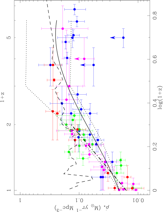
Figure 1: Evolution of SFR density with redshift, using a common obscuration correction where necessary. The points are color-coded by rest-frame wavelength as follows. Blue: UV; Green: [Oii]; Red: H$\alpha$ and H$\beta$; Pink: X-ray, FIR, sub-mm and radio. The solid line is the evolving 1.4 GHz LF derived by Haarsma et al. (2000). The dot-dashed line shows the least squares fit to all the $z<1$ data points, $\log(\dot{\rho}_{*})=3.10\log(1+z)-1.80$. The dotted lines show pure luminosity evolution for the Condon (1989) 1.4 GHz LF, at rates of $Q=2.5$ (lower) and $Q=4.1$ (upper). The dashed line is the “fossil” record from Local Group galaxies (Hopkins et al., 2001b).

The collection of measurements from the literature is presented in Table 2, with $\dot{\rho}_{*}$ given for both methods of obscuration correction, common and luminosity-dependent. The same values appear in both these columns for measurements not requiring obscuration correction (IR, sub-mm and radio), or for those where Balmer decrement measurements were used directly by the original authors to correct the data prior to deriving luminosity functions. This table also indicates the effective factors used in performing the cosmology correction from the original reference, and in both types of obscuration correction. A total of 33 references provide data here, giving a total of 66 points measured in the $(z,\dot{\rho}_{*})$ plane. These are shown in Figure 1. Of these points, 41 have measured obscuration corrections, are able to have an SFR-dependent obscuration correction applied, or have no need of obscuration corrections, and these results are shown in Figure 2. Adjacent data points from the [Oii] derived measurements of Hogg et al. (1998) are not independent, having been constructed in overlapping bins.

The LF parameters, where available, are given in Table 3 after converting to the cosmology assumed here. This table indicates whether the published LF includes obscuration corrections based on observed obscuration estimates or not. If not, integrations over these LFs are performed in order to apply the SFR-dependent obscuration correction detailed above. A fixed luminosity range is used for these integrations, depending on the wavelength at which the LF is estimated. For H$\alpha$ LFs, the integration is over $30.0\leq\log(L_{\rm H\alpha}/{\rm W})\leq 40.0$. For UV LFs the range is $15.0\leq\log(L_{\rm UV}/{\rm W\,Hz^{-1}})\leq 25$. For 1.4 GHz LFs the range is over $15.0\leq\log(L_{\rm 1.4}/{\rm W\,Hz^{-1}})\leq 28.0$. The data from the Great Observatories Origins Deep Survey (GOODS, Giavalisco et al., 2004), which include the two highest redshift UV-based data points, come from an integration of their derived luminosity functions that has an imposed absolute magnitude cutoff brighter than the limits assumed here for the other surveys. As a result the points corresponding to this survey shown in Figure 1 are actually lower limits to the total SFR density that would have been derived with the luminosity range indicated above. Integration of the LF over a magnitude range comparable with the above luminosity range is likely to increase these estimates by a factor of two or so. This would improve the level of consistency with the high redshift sub-mm measurement, and the evolving radio luminosity function results (see § 3 below). It is worth emphasising here, as an aside, that many high-redshift studies of the comoving SFR density (some of which are discussed further in § 5.2 below) impose a luminosity or magnitude limit on the integration of the LF, to avoid strong biases from the assumption of a faint end slope poorly constrained by observation. When comparing measurements in the literature it is obviously desirable to be consistent in the extent of the LF integrations being compared as, depending on the limits chosen, the results can vary by factors of two to four or so.

A common parameterisation for the evolution of the SFR density with redshift is a simple power law, $\dot{\rho}_{*}\propto(1+z)^{\beta}$, for $z\lesssim 1$, where $\beta$ has been estimated in the literature to range from around 1.5 (Cowie et al., 1999) to 3.9 (Lilly et al., 1996), with most favoured values around 3, for an Einstein-de Sitter (EdS) cosmology. The “meta-analysis” of Hogg (2002) gives a robust measurement of of $\beta=3.3\pm 0.8$ for an EdS cosmology, and a weighted mean fit of $\beta=2.74\pm 0.28$ for the cosmology assumed here. Using the current data compilation, restricted to measurements for $z\leq 1.0$, an ordinary least squares (OLS, Isobe et al., 1990) regression of $\log(\dot{\rho}_{*})$ on $\log(1+z)$ is performed to estimate both $\beta$ and $\log[\dot{\rho}_{*}(z=0)]$. For the assumption of a common obscuration this gives

$$\log(\dot{\rho}_{*})=(3.10\pm 0.25)\log(1+z)-(1.80\pm 0.04).$$ (3)

(Although both overlapping binnings for the data of Hogg et al., 1998, are shown in Figure 1, only the independent bins at $z=0.2,0.4,0.6,0.8,1.0$ have been used in this fit.) This result is consistent with that of Hogg (2002), although somewhat higher. The main reason for this is that the measurements of Mobasher et al. (1999) have been neglected in the current compilation. If that result is omitted from the analysis of Hogg (2002), a value of $\beta=3.15\pm 0.29$ would have been derived, highly consistent with the present estimate. The measurements of Mobasher et al. (1999) are omitted here primarily because of the significant incompleteness affecting their estimates, particularly for the higher redshift bin. For the case of the luminosity-dependent obscuration, the OLS regression gives

$$\log(\dot{\rho}_{*})=3.29\pm 0.26\log(1+z)-1.80\pm 0.04.$$ (4)

The consistency of these two results should not be too surprising, given that the 1.4 GHz and FIR derived data remain unchanged from one to the other. Both these relations are presented as dot-dashed lines in Figures 1 and 2 respectively. It is worth emphasising the similarity, though, between many of the data points at $z<1$ when corrected for obscuration using the two different methods. For these points the difference between the two different methods ranges from $\approx-20\%$ (Treyer et al., 1998; Tresse & Maddox, 1998), where the SFR dependent obscuration corrected value is lower than with the common obscuration, to $\approx+30\%$ (Connolly et al., 1997, the point at $z=0.75$).

2.5 Surface brightness dimming

The question of whether any given survey is complete over the full range of galaxy sizes for each interval of fixed luminosity is complex to address comprehensively. In most cases flux (or flux density) limits imposed in constructing source catalogues are effectively surface brightness thresholds (witness the so-called “resolution correction” made to radio galaxy source counts, e.g., Hopkins et al., 2003a, when constructed from peak flux density selected samples, to account for missing low surface brightness sources). Different methods used by different authors to address (or ignore) this issue, which affects both low and high redshift samples, may contribute to some extent to the scatter in the values seen for the estimated SFR density at each redshift.

Photometric redshifts have been used with large, deep samples of galaxies to estimate the SF history consistently over a very broad redshift range (Pascarelle et al., 1998; Lanzetta et al., 2002). The issue of correctly accounting for surface brightness dimming is of particular concern with this method, as a fixed flux limit corresponds to dramatically different surface brightness limits at different redshifts, and this can strongly bias the inferred SF history results. This problem is explored in detail by Lanzetta et al. (2002), in which the SFR intensity distribution, $h(x)$, is introduced. The evolution of $h(x)$ is explored by assuming three different models, one corresponding to luminosity evolution, one to a surface-density evolution, and an intermediate model defined by allowing the break point of the double-power-law distribution to evolve. The results of that analysis are shown in Figure 3, and presented in Table 4, after incorporating obscuration corrections using the common obscuration assumptions described above. It can be seen that the three models explored by Lanzetta et al. (2002) are highly consistent with the range of values measured in the other studies compiled here. The central model seems to be most consistent, and this is also apparently the most consistent with the data derived in Lanzetta et al. (2002) from the neutral hydrogen column density measured from damped Ly$\alpha$ absorption systems between redshifts $2.5<z<5$. There is also an apparent underestimate for all three models around $z\approx 1.5$ compared to the numerous other measurements in this region, as well as when compared to the lower limit inferred from the radio source counts, (lower dotted line, see § 3 below). There is also a continual increase above $z\approx 5$, counter to the assumptions made in the evolving radio LF modelling below. It is possible that the photometric redshift estimation erroneously identifies extreme redshifts (higher than $z\approx 6$ or 7) for objects whose true redshifts are around $z\approx 1.5$, where the 4000 Å break (an important feature in constraining photometric redshifts) is shifted out of the optical spectral window.

Apart from this issue, the SFR density evolution measured from photometric redshift estimates, when corrected for obscuration effects, appears highly consistent with all the other measurements and with the constraints from radio source counts. This is an encouraging result, suggesting that possible surface brightness related biases in the other estimates of SFR density compiled here are at most similar to the scatter seen between different measurements at similar redshifts. They may well be somewhat less given the other sources of uncertainty involved. This does not suggest that these effects should be ignored, but rather that more or less appropriate corrections have been used by most authors in accounting for these effects.

3 Evolving luminosity functions

In order to have a reference for interpreting these results and the overall compilation, evolving LFs for star forming (SF) galaxies have been explored.

Numerous measurements of evolutionary parameters or forms for galaxy LF exist in the literature. For the current exploration the evolving 1.4 GHz LF for star forming (SF) galaxies from Haarsma et al. (2000) is particularly relevant, as are the constraints on 1.4 GHz SF LF evolution from deep radio source counts (e.g., Hopkins et al., 1998; Rowan-Robinson et al., 1993). The SF history analysis of Haarsma et al. (2000) provides measurements at discrete redshifts in addition to the derived evolving LF. These points cannot be converted directly to the chosen SFR calibration, since this is luminosity-dependent. In order to be able to show these results, however, the ratio of each of these points to the measured evolving LF at the appropriate redshift was noted. These factors were then applied to the evolving LF after the cosmology and SFR calibration conversions, and the resulting data points are those given in Table 2 and shown in Figures 1 and 2. This is a somewhat coarse way to make the conversion, but it seems unlikely to have introduced an error of more than about $15\%$ given the locations of these points with respect to the nearby FIR data points from Flores et al (1999) both before and after the conversion.

To convert evolving LFs to the assumed cosmology, in order to compare with the current data compilation, the following relation is used (see discussion of Equation 4 from Dunlop & Peacock, 1990):

$$\phi_{1}(L_{1},z)\frac{dV_{c1}}{dz}=\phi_{2}(L_{2},z)\frac{dV_{c2}}{dz}$$ (5)

where $L_{1}$ is the luminosity derived from a given flux density and the luminosity distance corresponding to $z$ in the first cosmology, and $L_{2}$ is the luminosity derived from the same flux density with the luminosity distance for $z$ in the second cosmology. In other words, $L_{2}=L_{1}\times d_{l2}^{2}/d_{l1}^{2}$, with the $d_{l}$ being the luminosity distances in the respective cosmologies.

The evolving 1.4 GHz SF galaxy LFs, after the cosmology conversion, are converted to SFR densities at each redshift. This is done simply by integrating the LF at each redshift after converting luminosity to SFR. As well as the evolving LF of Haarsma et al. (2000), the local 1.4 GHz LF for SF galaxies from Condon (1989) is also used by invoking pure luminosity evolution, $L\propto(1+z)^{Q}$, having a cutoff at $z=2$. Constraints from faint radio source counts suggest that $2.5\lesssim Q\lesssim 4.1$ (e.g., Hopkins et al., 1998), and the evolution of the SFR density corresponding to these two extremes is calculated. The cosmology conversion in both cases is performed after the application of the appropriate evolutionary factors, since the derivation of these parameters was performed assuming an EdS cosmology. The resulting SF histories derived assuming $Q=2.5$ and $Q=4.1$ (in the EdS cosmology) are shown as dotted lines in Figures 1, 2 and 3.

4 Constraints on the LF evolution

The above comparisons illustrate the utility of the SF history to provide constraints on the form of the LF evolution for SF galaxies. Earlier studies have used the 1.4 GHz radio sources counts with some success to constrain the rate of pure luminosity evolution ($L\propto(1+z)^{Q}$) for the SF galaxy population (e.g., Rowan-Robinson et al., 1993; Hopkins et al., 1998; Seymour et al., 2004), while assuming no density evolution ($\phi\propto(1+z)^{P}$, with $P=0$). The constraints on these forms of evolution from radio source counts suffer from a degeneracy between luminosity and density evolution (Hopkins et al., 2003b) in the same fashion as found for the optical source counts (e.g., Lin et al., 1999). By itself, the SF history diagram, when used to constrain the evolution of the LF, suffers from a similar degeneracy. Together, though, the source counts and the star formation history can be combined to break this degeneracy, and this is explored here.

The local luminosity function for star forming galaxies of Sadler et al. (2002) was adopted. This was allowed to evolve assuming combinations of density evolution spanning $-6\leq P\leq 6$ in steps of 0.31, and luminosity evolution spanning $-1\leq Q\leq 7$ in steps of 0.21. In addition a cutoff in luminosity evolution was imposed above $z=2$ such that for higher redshifts $L\propto(1+2)^{Q}$. This is the same cutoff as used in earlier estimates of pure luminosity evolution (Rowan-Robinson et al., 1993; Hopkins et al., 1998). The constraint derived from the source counts does not turn out to depend strongly on this cutoff or, indeed, on the assumed cosmology (this was also recently shown by Seymour et al., 2004), although this is not true for the SF history constraint. For each value of $(P,Q)$ both the source counts and the star formation history were predicted and $\chi^{2}=\Sigma_{i}(y_{\rm model}-y_{i})^{2}/\sigma_{i}^{2}$ calculated. Here $y_{i}$ and $\sigma_{i}$ are either the source count measurements and uncertainties, respectively, or the SFR density measurements and uncertainties. The radio source counts used in the $\chi^{2}$ estimation are those from the Phoenix Deep Survey (PDS) data of Hopkins et al. (2003a) for flux densities $S_{1.4}<5\,$mJy and from the FIRST survey (White et al., 1997) for flux densities $3.1<S_{1.4}<502\,$mJy. In addition to the star forming galaxies, to fit the source counts an active galactic nucleus (AGN) population is also necessary. The evolving AGN LFs from Dunlop & Peacock (1990) were adopted, again as used in earlier studies, with appropriate cosmology conversion.

The SF history measurements used to estimate $\chi^{2}$, (where now each $y_{i}$ and $\sigma_{i}$ is an SFR density and uncertainty) are those derived using the common obscuration correction. Only the independent data points from Hogg et al. (1998) from this compilation were used, and the data point derived from Condon (1989) was excluded as its very small uncertainty otherwise dramatically affects the resulting $\chi^{2}$. The GOODS data points at high redshift were also excluded as they are effectively lower limits, due to the incomplete LF integration, as described above. The resulting $\chi^{2}$ arrays were converted to reduced $\chi^{2}$ values using 58 degrees of freedom (there are 6 parameters in the model, 4 from the LF and the 2 evolutionary parameters) for the source counts (with 64 measurements) and 48 for the SF history (with 54 measurements). These reduced $\chi^{2}$ arrays were then converted to log-likelihoods using $\log(L)\propto-0.5\chi^{2}$.

The joint likelihood for each $(P,Q)$ pair (assuming the measurements for the source counts and the SF history can be treated as independent) is simply the product of the likelihoods (the sum of the log-likelihoods) derived from the source counts and the SF history. The assumption of independence is not trivial, since both the SF history and the source counts involve integrations over the same luminosity function (weighted, in the case of the SF history, by the luminosity). For the SF history, the integration is over luminosity, while for the source counts it is over redshift. As an analogy, this can be thought of as taking a distribution of points in flux density/redshift space, and projecting them as distributions over either redshift or flux density. This would correspond to the integrations over flux density (or luminosity, for a fixed redshift), or redshift, respectively. If the distribution of points in flux density/redshift space is not correlated, the resulting projections are independent, and the corresponding probability distributions can be assumed to be independent. Since this is true for deep radio surveys such as the PDS, the assumption of independence is likely to be reasonable.

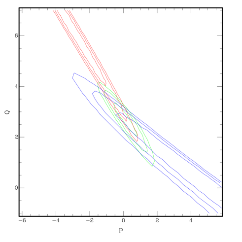
Figure 4: Probability contours showing $1\,\sigma$, $2\,\sigma$ and $3\,\sigma$ likelihood regions in the $P-Q$ plane. Blue contours are the constraint from the sub-mJy radio source counts, red are from the star formation history diagram, and green are the joint constraint.

Figure 4 shows the 1, 2 and $3\,\sigma$ contours for the constraints from both the source counts and the SF history, as well as the joint constraint. These contours are defined by subtracting 0.5, 1.0 and 1.5 respectively from the maximum of $\log(L)$, and the constraints from the SF history and the source counts seem to be consistent with each other at about the $2\,\sigma$ level. The maximum likelihood evolutionary parameters resulting from the joint constraint is $Q=2.70\pm 0.60$, $P=0.15\pm 0.60$.

To provide some further context for this result, the predicted redshift distributions for radio sources are shown in Figure 5, with the SF galaxy contribution derived assuming these rates of evolution. Four flux density limits are shown, ranging from 1 mJy, above which almost all radio sources are AGN dominated, to 0.05 mJy, the level to which the 1.4 GHz source counts are currently robustly measured, and where SF galaxies dominate the source numbers. It can be seen in Figure 5(d), corresponding to the flux density limit relevant for the current analysis, that SF galaxies dominate the distribution for redshifts below about $z\approx 0.7$, while AGNs contribute a significant proportion only at higher redshifts. This, along with the other limitations on this analysis at higher redshift (such as the assumed redshift cutoff in the SF galaxy evolution and the lack of a large number of SF history estimates), implies that the current analysis is perhaps less sensitive to the nature of galaxy evolution at high redshifts, and is constrained most strongly by the nature of low to moderate redshift SF galaxies. Altering the parameters of the assumed AGN luminosity function within a small range (constrained to retain the consistency with the observed radio source counts), for example, has the effect of modestly changing the shape of the predicted redshift distribution for the AGNs. Since these predominantly lie at high redshift and bright flux densities, the radio source count constraints for the evolution of the SF galaxy population are not significantly affected.

The assumed redshift cutoff in the SF galaxy evolution above $z=2$ can be seen as a sharp turnover in the SF galaxy numbers at this redshift, most noticable in Figure 5(c) and 5(d). This type of artifact is unlikely to appear in more realistic models of galaxy evolution and reflects the illustrative nature of the current investigation, which obviously leaves some room for refinement. The other aspect that must be taken into account in any interpretation of the distributions in this Figure is the effect of the optical counterpart brightness in constraining any observational redshift distributions that may be obtained. Models of bivariate radio-optical LFs and corresponding forms of evolution have been used to predict such distributions, (e.g., Hopkins, 1998; Hopkins et al., 1999), although such analysis is beyond the scope of the present work.

The likelihood contours for the SF history and source count constraints seen in Figure 4 show fairly well defined slopes, corresponding to degeneracies in $(P,Q)$. The reasons for these degeneracies can be understood in a little more detail by considering the dependence on $P$ and $Q$ of the calculations used to produce the SF history and the source counts. The source counts are considered here first, and can be written as:

$$SN(S)\propto\int dz\frac{dV_{c}}{dz}L\phi(L)$$ (6)

where $L=4\pi S[(1+z)D_{c}(z)]^{2}$, and $V_{c}=4\pi D_{c}^{3}/3$, and the subscript $c$ indicates the comoving distance or volume. The adopted forms for the luminosity and density evolution, $L^{*}(z)=L^{*}_{0}(1+z)^{Q}$ and $\phi^{*}(z)=\phi^{*}_{0}(1+z)^{P}$, mean that $L\phi(L)$ can be written as $(1+z)^{P}\phi^{*}_{0}f(y)$, where $y=L/L^{*}(z)$. Now, the comoving distance can be approximated as $D_{c}(z)=D_{EdS}(z)(1+z)^{\gamma}$ with the Einstein-de Sitter comoving distance $D_{EdS}(z)=2(c/H)(1-1/\sqrt{1+z})$, and $\gamma$ being a function of $\Omega$ and $\Lambda$. The expression $y$ is then a complicated function of $(1+z)$. Transforming the integral over $z$ into one over $y$ gives

$$SN(S)\propto\int dy{{dz}\over{dy}}{{dD_{c}}\over{dz}}{{dV_{c}}\over{dD_{c}}}\,(1+z)^{P}f(y).$$ (7)

Then, since

$$y = {{4\pi S}\over{L^{*}_{0}}}{{(1+z)^{2}\,D_{c}^{2}(z)}\over{(1+z)^{Q}}},$$

$${{dy}\over{dz}} = {{y}\over{1+z}}\left({{1}\over{\sqrt{1+z}-1}}+2\gamma+2-Q\right),$$

$${{dD_{c}}\over{dz}} = {{D_{c}(z)}\over{1+z}}{{1+2\gamma(\sqrt{1+z}-1)}\over{2(\sqrt{1+z}-1)}},\qquad{\rm and}$$

$${{dV_{c}}\over{dD_{c}}} = 4\pi D_{c}^{2},$$

the expression for the source counts becomes

$$SN(S) \propto \int{{dy}\over{2y}}\,f(y)\left[{{1+2\gamma(\sqrt{1+z}-1)}\over{1+(2\gamma+2-Q)(\sqrt{1+z}-1)}}\right]$$ (8)

$$\times(1+z)^{P}\,D_{c}^{3}.$$

This is a relation that can now be used to estimate the form of the degeneracy between $P$ and $Q$, given the observed source counts. The observed source count slope is close to Euclidean for small $z$, i.e., the differential source count $N(S)\propto S^{-5/2}$, or $SN(S)\propto S^{-3/2}$, and this should be independent of $z$ for small $z$. Now $D_{c}^{3}\propto(y/S)^{3/2}(1+z)^{3Q/2-3}$, and at small $z$ the term above in square brackets is $(1+\gamma z)/(1+(\gamma+1-Q/2)z)\approx(1+z)^{Q/2-1}$, so

$$SN(S)\propto\int{{dy}\over{2y}}\,\left({{y}\over{S}}\right)^{3/2}\,f(y)(1+z)^{P+3Q/2-3+Q/2-1},$$ (9)

at least in the regime in which the counts are dominated by objects at relatively small redshifts. Since there should be no dependence on $(1+z)$ in this regime, it might thus be expected that the constraint from the number counts scales as

$$P+2Q\approx 4.$$ (10)

This is independent of $\gamma$ since at small $z$ all cosmologies have similar $D_{c}(z)$ relations. The degeneracy indicated by the actual numerical estimates giving the likelihood contours in Figure 4 is $P+2Q\approx 5.4$. The difference from the scaling derived above is because, as might be expected, the contribution to the source counts from higher redshifts is not negligible.

The evolution of the SF history is somewhat simpler to understand. Since most SFR indicators are proportional to luminosity, $\dot{\rho}_{*}(z)$ is just the evolution of the luminosity density,

$$\dot{\rho}_{*}(z) \propto \int dL\,\phi(L|z)\,L$$ (11)

$$\propto L^{*}(z)\int dL\,\phi(L|z)\,{{L}\over{L^{*}(z)}}$$

$$\propto L^{*}_{0}\,(1+z)^{Q}\,\phi^{*}_{0}\,(1+z)^{P}\,\int dy\,f(y).$$

The observed slope of $\log{\dot{\rho}_{*}(z)}$ with $\log(1+z)$ thus constrains the value of the sum $(P+Q)$. This slope has been seen to be about 3 (up to $z=1$), so $P+Q\approx 3$, which is in excellent agreement with the degeneracy in $(P,Q)$ seen in Figure 4 for the SF history likelihood contours.

This analysis suggests that there are understandable reasons for the degeneracies seen between $P$ and $Q$, and the measurements are consistent with what might be expected from this analysis. The form of the degeneracies are fortunately different for the source counts and the SF history, and the degeneracies can be broken by combining these constraints. More detailed investigation along these lines might usefully identify additional observables that could similarly be used to break such degeneracies, yet further constraining the form of evolution of the star forming galaxy luminosity function.

5 Discussion

5.1 Limitations of this analysis

There appears to be a large discrepancy (factors of two) in the local SFR density derived from integrating various local radio LFs. When the actual LFs are compared, however, the measurements are highly consistent (compare, e.g., the LF and parameterisations of Sadler et al. (2002) and Machalski & Godlowski (2000)). The discrepancy here occurs because of the different LF parameters derived, (even for the same functional form), which when integrated over the complete luminosity range give different results. This is in part a contribution of the poorly constrained tails of the LFs, but there is also a contribution from the different values for $L^{*}$ which translate to different locations for the peak in the luminosity density as a function of luminosity, and hence to the derived total SFR densities. It is known that LF parameters are not independent, and the effect of this is that the uncertainty in the LF integral requires the incorporation of the LF parameter error ellipse, in addition to the Poisson uncertainties typically quoted. The result is that at least some of the scatter in the SF history diagram will be due to different choices for LF parameterisation (not only for radio LFs, but also at other wavelengths).

This systematic uncertainty is clearly not accounted for in the published uncertainties for the SFR density measurements. These typically reflect only assumed Poisson counting uncertainties, while neglecting other systematics that may be important for any particular survey, typically because these effects are difficult to quantify. As a result the quoted uncertainties for most data points are likely to be lower limits to the true uncertainties. This has not been accounted for in the $\chi^{2}$ calculations used above to constrain the SF galaxy LF evolution. One way to minimise any bias introduced by this issue might be to bin the measured SFR density points in redshift, summing in quadrature their published uncertainties. By combining adjacent data points as an average or median, the most extreme outlying points as well as those with the least representative uncertainties, will have their disproportionate effects on the $\chi^{2}$ statistic minimised. This has been explored using several different binnings of the data, ranging from including as few as 5 points per bin to as many as 8 points per bin (coarser binning leaves the problem unconstrained as there are then fewer data points than free parameters, while finer binning eliminates the advantage of this method as there are then too few points per bin to smooth out the more extreme measurements). The joint constraint with the source counts when using this method is changed only marginally, although the likelihood peak in the constraint from the SF history alone moves along the line of degeneracy to smaller $Q$ and larger $P$ values. This suggests that the apparent marginal consistency (at the $2\,\sigma$ level) between the SF history and source count datasets separately is likely to be an artifact of a few measurements contributing disproportionately to the $\chi^{2}$ estimate for the former, and the true consistency could be much better.

The preferred value for the luminosity evolution, $Q=2.70\pm 0.60$, is highly consistent with a recent estimate from models incorporating luminosity evolution only (no density evolution) when constrained by the 1.4 GHz source counts (Seymour et al., 2004). It is worth noting, though, that is somewhat lower than the fitted slope to the SF history data points for $z<1$, $\beta=3.10\pm 0.25$. This cannot be completely explained by the small contribution from the density evolution ($P=0.15\pm 0.60$), since even together these effects produce a slightly flatter slope compared with $\beta$. This is a result both of including points at $z>1$ in the $\chi^{2}$ calculation as well as the effect of the constraint from the source counts (the constraint from the SF history alone seems to favour somewhat higher values of $Q$ with negative values for $P$). Regarding the choice of local SF galaxy LF for the investigation of the evolutionary parameters, choosing a different LF from that of Sadler et al. (2002) would produce slightly different results for the best-fitting values of $(P,Q)$. The LF from Condon et al. (2002) (producing one of the lowest values for the local SFR density) would favour somewhat higher rates of luminosity or density evolution, and a correspondingly steeper slope in the global SF history diagram. When the constraints from the source counts are incorporated, though, the resulting preferred values still do not change much from those derived above.

Apart from the factors of two uncertainty in the local estimate for the SFR density, the other most strikingly outlying points include the lowest redshift UV-derived points (Sullivan et al., 2000; Treyer et al., 1998), and the [Oii] data from Hogg et al. (1998). The latter is explained by that author simply as the effect of the small numbers contributing to each redshift bin, and the choice of bin location (prompting the use of the overlapping bins chosen to emphasise the extent of this effect). The UV-derived estimates at $z=0.15$ appear to be high compared with other estimates from H$\alpha$, [Oii] or radio luminosities at similar redshifts. It is likely that this is actually a result of an overestimated obscuration correction, both with the common obscuration and the SFR-dependent obscuration methods used, which can be seen to produce similar corrections. The underlying reason for this is a combination of lower luminosity systems having lower obscurations, and low-redshift UV-selected samples being dominated primarily by such relatively low luminosity systems. This is supported by the fact that the SFR density derived for the samples of Tresse & Maddox (1998) and Treyer et al. (1998) using the SFR dependent obscuration gives a lower value than that using the common obscuration correction. Further, as can be seen from Figure 1 of Sullivan et al. (2000), for example, although the mean obscuration is close to $A_{V}=1\,$mag for this sample, the median is somewhat lower (probably closer to $A_{V}=0.8\,$mag). The effective obscuration correction for this sample, in terms of a common obscuration, should thus be somewhat lower than assumed. For the luminosity-dependent obscuration, similarly, the curve from Hopkins et al. (2001a) is again less appropriate, having been derived from a sample containing more heavily obscured systems at all luminosities than are likely to be found in the local UV-selected samples. When these effects are accounted for, the UV-derived points at $z=0.15$ will be moved lower, more consistent with the rest of the compilation around this redshift.

5.2 The shape of the $z>3$ SF history

Recent investigations of $z\approx 6$ $i^{\prime}$-band dropouts have suggested that the SF history is steadily dropping from $z=3$ to $z\approx 6$ (Bouwens et al., 2003; Fontana et al, 2003; Stanway et al., 2004). These analyses compare the comoving SFR density for objects with high SFRs ($\gtrsim 15\,M_{\odot}$yr^-1, Stanway et al., 2004), and find a decrease in this SFR density of almost an order of magnitude from $z=3$ to $z\approx 6$. The reason for limiting the analysis to objects with high SFRs is to avoid the extrapolations made in assuming a particular faint end slope ($\alpha$) for the LF. If the faint end slope is assumed to be $\alpha=-1.6$ (Yan et al., 2003; Bouwens et al., 2003), and the LF integrated over all luminosities, the derived SFR density is a factor of about four greater than for just the high SFR objects alone (Bouwens et al., 2003). The value established assuming this faint end slope by Bouwens et al. (2003) (after conversion to the UV SFR calibration adopted here) is $0.04\,M_{\odot}$yr^-1. If obscuration corrections are then made (assuming the common obscuration correction used herein), the SFR density is increased by another factor of about 3.4, to $0.14\,M_{\odot}$yr^-1 at $z\approx 6$, highly consistent with the other estimates shown in Figure 1. It should be emphasised that the estimated $\approx 40\%$ decrease in comoving SFR density from $z=3$ to $z\approx 6$ claimed by Bouwens et al. (2003) lies entirely within the scatter of the measurement compilation, and associated uncertainties, over this redshift range. The much lower $z\approx 6$ SFR densities derived by Fontana et al (2003) and Stanway et al. (2004), indicating an order of magnitude drop from $z=3$, are less consistent, being significantly lower than the estimates of Bouwens et al. (2003). These apparent inconsistencies are related to the small numbers of objects in the samples (at most about 30, with as few as 6 galaxies contributing to some analyses), the assumptions involved in correcting for incompleteness, and the uncertainty in the faint end slope of the luminosity function. Requiring an absolute magnitude limited sample, for example, seems to imply constant SFR densities up to $z\approx 6$ (Fontana et al, 2003). There is evidence, too, for faint end LF slopes as steep as $\alpha=-1.6$ or steeper (Yan et al., 2003) at these redshifts, which would also support relatively little evolution.

Given these uncertainties, it is clear that larger samples are needed at these high redshifts, probing to fainter luminosities to robustly determine the faint end slope of the LF, before it is possible to reliably constrain the shape of the SFR density evolution beyond $z\approx 3$.

6 Summary

An extensive compilation from the literature of SFR density measurements as a function of redshift has been presented. These data have been converted to a consistent set of SFR calibrations, common cosmology, and consistent dust obscuration corrections where necessary. The compilation thus produced gives a highly consistent description of the evolution in galaxy SFR density with redshift, constrained to within factors of about three at most redshifts up to $z\approx 6$. In producing this compilation, different assumptions regarding obscuration have been explored. For those measurements requiring obscuration corrections the assumptions used were those deemed most likely to be appropriate. Alternative assumptions regarding the obscuration corrections, however, will act to increase the SFR densities derived compared with those presented here (with the possible exception of the poorly known obscuration properties of high redshift systems, $z\gtrsim 1$).

This rich compilation of SFR density evolution provides a robust constraint for many investigations of galaxy evolution, and this has been illustrated by constraining the evolution of the SF galaxy LF. In combination with constraints from the radio source counts, the SF galaxy LF is found to evolve with luminosity and density evolutionary parameters $Q=2.70\pm 0.60$ and $P=0.15\pm 0.60$ respectively. An analysis has been performed of the degeneracies between $P$ and $Q$ seen in the separate constraints from the source counts and the SF history. This suggests that the origin of these degeneracies is reasonably well understood, and this methodology may be a useful tool for identifying additional observables that could be used as additional constraints for breaking such degeneracies.

While every effort has been made to be as thorough as possible in the current compilation, it is possible that some datasets or measurements may have been inadvertently omitted. It seems unlikely, though, that such omissions will significantly alter the above conclusions. At the same time, it is the author’s hope that a complete and expansive review of this topic (more so than possible in the present case) will be able to do justice to the wealth of current and ongoing measurements contributing to our understanding of this aspect of galaxy evolution.

Table 1: SFR calibrations. SFR is in units of $M_{\odot}\,$yr^-1. 1.4 GHz and UV luminosities are in units of W Hz^-1. FIR and H$\alpha$ luminosities are in units of W.

Wavelength	Calibration
1.4 GHz	${\rm SFR}=\left\{\begin{array}[]{l}L_{1.4}/1.81\times 10^{21}\hskip 140.84114ptL_{1.4}>6.4\times 10^{21}\,{\rm W\,Hz}^{-1}\\ L_{1.4}/[1.81\times 10^{21}(0.1+0.9(L_{1.4}/6.4\times 10^{21})^{0.3}]\hskip 8.53581ptL_{1.4}<6.4\times 10^{21}\,{\rm W\,Hz}^{-1}\end{array}\right.$
FIR	${\rm SFR}=L_{\rm FIR}/2.22\times 10^{36}$
H$\alpha$	${\rm SFR}=L_{\rm H\alpha}/1.26\times 10^{34}$
UV	${\rm SFR}=L_{\rm UV}/7.14\times 10^{20}$

Table 2: Measurements of SFR density, $\dot{\rho}_{*}$, in units of $M_{\odot}\,$yr^-1 Mpc^-3, as a function of redshift.

Reference	Estimator	Redshift	$C_{1}$	$\log(\dot{\rho}_{*{\rm com}})\tablenotemark{b}$	$C_{2}$	$\log(\dot{\rho}_{*{\rm sfrd}})\tablenotemark{d}$	$C_{3}$
Giavalisco et al. (2004)	1500 Å	$3.780\pm 0.340$	1.0	$-0.772\pm 0.060$	…
		$4.920\pm 0.330$	1.0	$-0.963\pm 0.140$	…
		$5.740\pm 0.360$	1.0	$-0.923\pm 0.190$	…
Wilson et al. (2002)	2500 Å	$0.350\pm 0.150$	1.0	$-1.449\pm 0.078$	2.53	$-1.366\pm 0.097$	3.06
		$0.800\pm 0.200$	1.0	$-1.183\pm 0.080$	2.53	$-1.129\pm 0.043$	2.87
		$1.350\pm 0.250$	1.0	$-1.034\pm 0.143$	2.53	$-1.016\pm 0.093$	2.64
Massarotti et al. (2001)	1500 Å	$1.500\pm 0.500$	0.822	$-0.709\pm 0.200$	…	$-0.709\pm 0.200$	…
		$2.750\pm 0.750$	0.784	$-0.512\pm 0.200$	…	$-0.512\pm 0.200$	…
		$4.000\pm 0.500$	0.774	$-0.886\pm 0.250$	…	$-0.886\pm 0.250$	…
Sullivan et al. (2000)	2000 Å	$0.150\pm 0.150$	0.611	$-1.403\pm 0.050$	2.86	$-1.402\pm 0.050$	2.87
Steidel et al. (1999)	1700 Å	$3.040\pm 0.250$	0.389	$-0.795\pm 0.050$	3.15	$-0.585\pm 0.050$	5.11
		$4.130\pm 0.300$	0.387	$-0.905\pm 0.100$	3.15	$-0.693\pm 0.100$	5.13
Cowie et al. (1999)	2000 Å	$0.700\pm 0.200$	0.717	$-1.318\pm 0.104$	2.86	$-1.316\pm 0.052$	2.88
		$1.250\pm 0.250$	0.646	$-1.186\pm 0.117$	2.86	$-1.057\pm 0.060$	3.86
Treyer et al. (1998)	2000 Å	$0.150\pm 0.150$	0.611	$-1.369\pm 0.150$	2.86	$-1.439\pm 0.150$	2.44
Connolly et al. (1997)	2800 Å	$0.750\pm 0.250$	0.917	$-0.992\pm 0.150$	2.37	$-0.887\pm 0.150$	3.01
		$1.250\pm 0.250$	0.841	$-0.864\pm 0.150$	2.37	$-0.679\pm 0.150$	3.63
		$1.750\pm 0.250$	0.812	$-0.974\pm 0.150$	2.37	$-0.717\pm 0.150$	4.29
Lilly et al. (1996)	2800 Å	$0.350\pm 0.150$	1.07	$-1.539\pm 0.070$	2.37
		$0.625\pm 0.125$	0.953	$-1.266\pm 0.080$	2.37
		$0.875\pm 0.125$	0.892	$-0.979\pm 0.150$	2.37
Madau et al. (1996)	1600 Å	$2.750\pm 0.750$	0.784	$>-1.217$	3.27
		$4.000\pm 0.500$	0.774	$>-1.723$	3.27
Teplitz et al. (2003)	[Oii]	$0.900\pm 0.500$	1.0	$-1.005\pm 0.110$	2.51	$-0.902\pm 0.110$	3.18
Gallego et al. (2002)	[Oii]	$0.025\pm 0.025$	0.677	$-1.913\pm 0.150$	…	$-1.913\pm 0.150$	…
Hogg et al. (1998)	[Oii]	$0.200\pm 0.100$	0.588	$-1.640^{+0.163}_{-0.118}$	2.51
		$0.300\pm 0.100$	0.551	$-1.712^{+0.101}_{-0.094}$	2.51
		$0.400\pm 0.100$	0.522	$-1.067^{+0.105}_{-0.085}$	2.51
		$0.500\pm 0.100$	0.499	$-0.826^{+0.075}_{-0.067}$	2.51
		$0.600\pm 0.100$	0.480	$-1.003^{+0.072}_{-0.062}$	2.51
		$0.700\pm 0.100$	0.466	$-1.094^{+0.088}_{-0.073}$	2.51
		$0.800\pm 0.100$	0.454	$-1.076^{+0.081}_{-0.071}$	2.51
		$0.900\pm 0.100$	0.444	$-0.982^{+0.090}_{-0.074}$	2.51
		$1.000\pm 0.100$	0.436	$-0.783^{+0.107}_{-0.087}$	2.51
		$1.100\pm 0.100$	0.429	$-0.893^{+0.199}_{-0.136}$	2.51
		$1.200\pm 0.100$	0.423	$-0.919^{+0.301}_{-0.176}$	2.51
Hammer et al. (1997)	[Oii]	$0.375\pm 0.125$	1.06	$-1.705^{+0.070}_{-0.080}$	2.51
		$0.625\pm 0.125$	0.953	$-1.226^{+0.110}_{-0.150}$	2.51
		$0.875\pm 0.125$	0.892	$-0.855^{+0.200}_{-0.380}$	2.51
Pettini et al. (1998)	H$\beta$	$2.750\pm 0.750$	0.784	$-0.557\pm 0.150$	3.71
Pérez-González et al. (2003)	H$\alpha$	$0.025\pm 0.025$	1.0	$-1.604\pm 0.110$	…	$-1.604\pm 0.110$	…
Tresse et al. (2002)	H$\alpha$	$0.700^{+0.400}_{-0.200}$	0.933	$-0.931\pm 0.110$	2.51	$-0.933\pm 0.110$	2.50
Moorwood et al. (2000)	H$\alpha$	$2.200\pm 0.050$	0.790	$-0.576\pm 0.120$	2.51	$-0.426\pm 0.120$	3.54
Hopkins et al. (2000)	H$\alpha$	$1.250\pm 0.550$	0.561	$-0.629\pm 0.026$	2.51	$-0.588\pm 0.064$	2.76
Sullivan et al. (2000)	H$\alpha$	$0.150\pm 0.150$	0.611	$-1.820\pm 0.060$	…	$-1.820\pm 0.060$	…
Glazebrook et al. (1999)	H$\alpha$	$0.900\pm 0.100$	0.89	$-0.972^{+0.150}_{-0.140}$	…
Yan et al. (1999)	H$\alpha$	$1.300\pm 0.600$	0.837	$-0.553\pm 0.120$	2.51	$-0.412\pm 0.120$	2.41
Tresse & Maddox (1998)	H$\alpha$	$0.200\pm 0.100$	1.17	$-1.489\pm 0.060$	2.51	$-1.571\pm 0.060$	2.09
Gallego et al. (1995)	H$\alpha$	$0.022\pm 0.022$	1.37	$-1.900\pm 0.200$	…	$-1.900\pm 0.200$	…
Flores et al (1999)	$15\,\mu$m	$0.350\pm 0.150$	1.07	$-1.438\pm 0.270$	…	$-1.438\pm 0.270$	…
		$0.625\pm 0.125$	0.953	$-1.169\pm 0.250$	…	$-1.169\pm 0.250$	…
		$0.875\pm 0.125$	0.892	$-0.874\pm 0.260$	…	$-0.874\pm 0.260$	…
Barger et al. (2000)	$850\,\mu$m	$2.000\pm 1.000$	0.615	$-0.831^{+0.220}_{-0.230}$	…	$-0.831^{+0.220}_{-0.230}$	…
		$4.500\pm 1.500$	0.594	$-0.721^{+0.360}_{-0.430}$	…	$-0.721^{+0.360}_{-0.430}$	…
Hughes et al. (1998)	$850\,\mu$m	$3.000\pm 1.000$	0.39	$>-1.087\pm 0.170$	…
Condon et al. (2002)	1.4 GHz	$0.005\pm 0.005$	1.0	$-1.964\pm 0.030$	…	$-1.964\pm 0.030$	…
Sadler et al. (2002)	1.4 GHz	$0.080\pm 0.080$	1.30	$-1.728^{+0.080}_{-0.090}$	…	$-1.728^{+0.080}_{-0.090}$	…
Serjeant et al. (2002)	1.4 GHz	$0.010\pm 0.010$	1.39	$-1.753^{+0.080}_{-0.100}$	…	$-1.753^{+0.080}_{-0.100}$	…
Machalski &	1.4 GHz	$0.070\pm 0.070$	1.31	$-1.920\pm 0.100$	…	$-1.920\pm 0.100$	…
Godlowski (2000)
Haarsma et al. (2000)	1.4 GHz	$0.280^{+0.121}_{-0.270}$	0.60	$-1.389^{+0.140}_{-0.210}$	…	$-1.389^{+0.140}_{-0.210}$	…
		$0.460^{+0.058}_{-0.050}$	0.52	$-1.176^{+0.140}_{-0.200}$	…	$-1.176^{+0.140}_{-0.200}$	…
		$0.600^{+0.098}_{-0.052}$	0.48	$-1.117^{+0.160}_{-0.260}$	…	$-1.117^{+0.160}_{-0.260}$	…
		$0.810^{+0.074}_{-0.086}$	0.44	$-0.881^{+0.130}_{-0.180}$	…	$-0.881^{+0.130}_{-0.180}$	…
		$1.600^{+2.820}_{-0.640}$	0.40	$-0.785^{+0.120}_{-0.180}$	…	$-0.785^{+0.120}_{-0.180}$	…
Condon (1989)	1.4 GHz	$0.005\pm 0.005$	1.55	$-1.679\pm 0.001$	…	$-1.679\pm 0.001$	…
Georgakakis et al. (2003)	X-ray	$0.24^{+0.06}_{-0.24}$	0.88	$-1.417^{+0.219}_{-0.182}$	…	$-1.417^{+0.219}_{-0.182}$	…
	($0.5-2\,$keV)

Table 3: Luminosity function parameters, converted to the currently assumed cosmology.

Reference	$z$	$\log(L^{*})$	$\phi^{*}$	$\alpha$	$\sigma$	Note
Wilson et al. (2002)	0.35	21.182, 21.806	$5.52$, $1.06$	$-1.0$, $-1.5$	…
	0.80	21.286, 21.474	$7.96$, $4.22$	$-1.0$, $-1.5$	…
	1.35	21.198, 21.290	$11.9$, $10.5$	$-1.0$, $-1.5$	…
Sullivan et al. (2000)	0.15	21.342	$2.48$	$-1.51$	…
Steidel et al. (1999)	3.04	22.072	$1.39$	$-1.6$	…
	4.13	22.076	$1.07$	$-1.6$	…
Cowie et al. (1999)	0.70	21.05, 21.17	$8.4$, $5.8$	$-1.0$, $-1.5$	…
	1.25	21.48, 21.56	$4.1$, $3.3$	$-1.0$, $-1.5$	…
Treyer et al. (1998)	0.15	21.285	$2.37$	$-1.62$	…
Connolly et al. (1997)	0.75	21.65	$5.30$	$-1.3$	…
	1.25	22.01	$3.10$	$-1.3$	…
	1.75	22.35	$1.10$	$-1.3$	…
Teplitz et al. (2003)	0.90	35.60	$0.90$	$-1.35$	…	1.
Gallego et al. (2002)	0.025	36.33	$0.0636$	$-1.17$	…	1., 2.
Pérez-González et al. (2003)	0.025	35.43	$1.00$	$-1.2$	…	2.
Tresse et al. (2002)	0.7	34.97	$4.80$	$-1.31$	…
Moorwood et al. (2000)	2.2	35.88	$1.27$	$-1.35$	…	3.
Hopkins et al. (2000)	1.25	35.87, 36.34	$0.766$, $0.088$	$-1.60$, $-1.86$	…
Sullivan et al. (2000)	0.15	35.42	$0.313$	$-1.62$	…	2.
Yan et al. (1999)	1.3	35.83	$1.50$	$-1.35$	…
Tresse & Maddox (1998)	0.20	34.61	$2.89$	$-1.35$	…
Gallego et al. (1995)	0.0225	34.87	$1.65$	$-1.3$	…	2.
Sadler et al. (2002)	0.08	19.29	$22.9$	$0.84$	0.94	4.
Serjeant et al. (2002)	0.01	22.16	$1.32$	$-1.29$	…
Machalski & Godlowski (2000)	0.07	21.468	$2.38$	$1.22$	0.61	4.

Note. — Units of $L^{*}$ are W for H$\alpha$ LFs, or W Hz^-1 for UV or 1.4 GHz LFs. Units of $\phi^{*}$ are $10^{-3}$ Mpc^-3. The 1.4 GHz LFs from Condon et al. (2002) and Condon (1989) use a parameterisation corresponding to “hyperbolic” visibility functions. These are parameterised using $Y=3.06$, $B=1.9$, $X=22.35$, $W=0.67$ (for Condon et al., 2002) and $Y=2.88$, $B=1.5$, $X=22.108$, $W=0.667$ (for Condon, 1989), after conversion to the currently assumed cosmology.

1. Effective H$\alpha$ LF inferred from observed [Oii] LF.

2. Obscuration corrected by original authors using measured values of obscuration for individual objects.

3. This LF was not fitted to the observations. Rather the observations at $z=2.2$ appear consistent with the $z=1.3$ LF of Yan et al. (1999), in the cosmologies assumed by those authors, so that LF is adopted for this higher redshift. Note that the cosmology conversions at the different redshifts give rise to different $L^{*}$ and $\phi^{*}$ values for the currently assumed cosmology.

4. The form of the LF here is that of Saunders et al. (1990), where $\alpha$ has a slightly different definition from that in the Schechter (1976) LF, and the $\sigma$ parameter effectively broadens the bright end of the LF.

Table 4: Measurements of $1500\,$Å SFR density based on photometric redshift estimation in the HDF and HDF-S.

Redshift	$\log(\dot{\rho}_{*})$	$\log(\dot{\rho}_{*})$	$\log(\dot{\rho}_{*})$	$\log(\dot{\rho}_{*})$
	Pascarelle et al. (1998)		Lanzetta et al. (2002)
$0.25\pm 0.25$	$-1.242^{+0.310}_{-0.220}$	$-1.807^{+0.041}_{-0.058}$	$-1.760^{+0.030}_{-0.023}$	$-1.713^{+0.023}_{-0.041}$
$0.75\pm 0.25$	$-1.195^{+0.230}_{-0.140}$	$-1.631^{+0.029}_{-0.059}$	$-1.543^{+0.017}_{-0.053}$	$-1.526^{+0.018}_{-0.064}$
$1.25\pm 0.25$	$-1.042^{+0.240}_{-0.120}$	$-1.526^{+0.024}_{-0.093}$	$-1.485^{+0.029}_{-0.053}$	$-1.456^{+0.018}_{-0.093}$
$1.75\pm 0.25$	$-1.030^{+0.240}_{-0.120}$	$-1.508^{+0.035}_{-0.059}$	$-1.473^{+0.023}_{-0.041}$	$-1.391^{+0.046}_{-0.053}$
$2.25\pm 0.25$		$-1.152^{+0.030}_{-0.076}$	$-1.000^{+0.023}_{-0.064}$	$-0.690^{+0.070}_{-0.070}$
$2.50\pm 0.50$	$-1.251^{+0.280}_{-0.210}$
$2.75\pm 0.25$		$-1.181^{+0.035}_{-0.082}$	$-0.883^{+0.035}_{-0.053}$	$-0.526^{+0.129}_{-0.175}$
$3.50\pm 0.50$	$-1.288^{+0.340}_{-0.270}$	$-1.040^{+0.035}_{-0.094}$	$-0.585^{+0.058}_{-0.064}$	$-0.082^{+0.175}_{-0.316}$
$4.50\pm 0.50$	$-1.180^{+0.440}_{-0.370}$	$-1.052^{+0.035}_{-0.094}$	$-0.567^{+0.088}_{-0.094}$	$-0.058^{+0.228}_{-0.415}$
$5.50\pm 0.50$	$-1.542^{+0.590}_{-0.380}$	$-0.977^{+0.070}_{-0.093}$	$-0.433^{+0.199}_{-0.275}$	$0.158^{+0.357}_{-0.918}$
$8.00\pm 2.00$		$-0.784^{+0.064}_{-0.111}$	$-1.088^{+0.228}_{-0.322}$	$0.678^{+0.386}_{-0.865}$

Figure 3: Lines are as in previous Figures, although note the different scales on the axes. The points show the data from Figure 4 of Lanzetta et al. (2002) (circles correspond to the green data points of that Figure, squares to the blue points and triangles to the red points), after correction for a common obscuration. This emphasises the high level of consistency between the current compilation and the UV estimates at high redshift, even when the effects of surface brightness dimming are taken into account.

Figure 5: Redshift distributions predicted from the evolving radio LFs for four different radio flux density limits. The SF galaxy LF assumes the best-fitting luminosity and density evolution derived from the previous Figure ($Q=2.70$, $P=0.15$). In each panel the dot-dashed line is the contribution from AGN galaxies, the dashed line is that from SF galaxies, and the solid line is the total galaxy redshift distribution.

References

- Afonso et al. (2003) Afonso, J., Hopkins, A., Mobasher, B., Almeida, C. 2003, ApJ, 597, 269
- Aragón-Salamanca et al. (2002) Aragón-Salamanca, A., Alonso-Herrero, A., Gallego, J., García-Dabó, C. E., Pérez-González, P. G., Zamorano, J., Gil de Paz, A. 2002, in “Star Formation through Time” (astro-ph/0210123)
- Ascasibar et al. (2002) Ascasibar, Y., Yepes, G., Gottlöber, S., Müller, V. 2002, A&A, 387, 396
- Barger et al. (2000) Barger, A. J., Cowie, L. L., Richards, E. A. 2000, AJ, 119, 2092
- Bell (2003) Bell, E. 2003, ApJ, 586, 794
- Bouwens et al. (2003) Bouwens, R. J., et al. 2003, ApJ, 595, 589
- Buat et al. (2002) Buat, V., Boselli, A., Gavazzi, G., Bonfanti, C. 2002, A&A, 383, 801
- Calzetti (2001) Calzetti, D. 2001, PASP, 113, 1449
- Calzetti et al. (2000) Calzetti, D., Armus, L., Bohlin, R. C., Kinney, A. L., Koornneef, J., Storchi-Bergmann, T. 2000, ApJ, 533, 682
- Calzetti et al. (1996) Calzetti, D., Kinney, A. L., Storchi-Bergmann, T. 1996, ApJ, 458, 132
- Cardelli et al. (1989) Cardelli, J. A., Clayton, G. C., Mathis, J. S. 1989, ApJ, 345, 245
- Condon (1989) Condon, J. J. 1989, ApJ, 338, 13
- Condon (1992) Condon, J. J. 1992, ARA&A, 30, 575
- Condon et al. (2002) Condon, J. J., Cotton, W. D., Broderick, J. J. 2002, AJ, 124, 675
- Connolly et al. (1997) Connolly, A. J., Szalay, A. S., Dickinson, M., SubbaRao, M. U., Brunner, R. J. 1997, ApJ, 486, L11
- Cowie et al. (1999) Cowie, L. L., Songaila, A., Barger, A. J. 1999, AJ, 118, 603
- Dunlop & Peacock (1990) Dunlop, J. S., Peacock, J. A. 1990, MNRAS, 247, 19
- Flores et al (1999) Flores, H., et al. 1999, ApJ, 517, 148
- Fontana et al (2003) Fontana, A., Poli, F., Menci, N., Nonino, M., Giallongo, E., Cristiani, S., D’Odorico, S. 2003, ApJ, 587, 544
- Gallego et al. (2002) Gallego, J., García-Dabó, C. E., Zamorano, J., Aragón-Salamanca, A., Rego, M. 2002, ApJ, 570, L1
- Gallego et al. (1996) Gallego, J., Zamorano, J., Alonso, O., Vitores, A. G. 1996, A&AS, 120, 323
- Gallego et al. (1995) Gallego, J., Zamorano, J., Aragón-Salamanca, A., Rego, M. 1995, ApJ, 455, L1
- Georgakakis et al. (2003) Georgakakis, A., Hopkins, A. M., Sullivan, M., Afonso, J., Georgantopoulos, I., Mobasher, B., Cram, L. 2003, MNRAS, 345, 939
- Giavalisco et al. (2004) Giavalisco, M., et al. 2004, ApJ, 600, L103
- Glazebrook et al. (1999) Glazebrook, K., Blake, C., Economou, F., Lilly, S., Colless, M. 1999, MNRAS, 306, 843
- Haarsma et al. (2000) Haarsma, D. B., Partridge, R. B., Windhorst, R. A., Richards, E. A. 2000, ApJ, 544, 641
- Hammer et al. (1997) Hammer, F., et al. 1997, ApJ, 481, 49
- Hogg (2002) Hogg, D. W. 2002, PASP(submitted; astro-ph/0105280)
- Hogg et al. (1998) Hogg, D. W., Cohen, J. G., Blandford, R., Pahre, M. A. 1998, ApJ, 504, 622
- Hopkins (1998) Hopkins, A. M., PhD Thesis, 1998, University of Sydney
- Hopkins et al. (2003c) Hopkins, A. M., et al. 2003c, ApJ, 599, 971
- Hopkins et al. (2003a) Hopkins, A. M., Afonso, J., Chan, B., Cram, L. E., Georgakakis, A., Mobasher, B. 2003a, AJ, 125, 465
- Hopkins et al. (2003b) Hopkins, A. M., Afonso, J., Georgakakis, A., Sullivan M., Cram, L. E., Mobasher, B. 2003b, in “Multiwavelength Galaxy Evolution” Mykonos, (astro-ph/0309147)
- Hopkins et al. (2001a) Hopkins, A. M., Connolly, A. J., Haarsma, D. B., Cram, L. E. 2001a, AJ, 122, 288
- Hopkins et al. (1999) Hopkins, A. M., Cram L., Mobasher B., Georgakakis A., 1999, in “Looking Deep in the Southern Sky” eds. R. Morganti & W.J. Couch, (Springer:Berlin), 120
- Hopkins et al. (2000) Hopkins, A. M., Connolly, A. J., Szalay, A. S. 2000, AJ, 120, 2843
- Hopkins et al. (2001b) Hopkins, A. M., Irwin, M. J., Connolly, A. J. 2001b, ApJ, 558, L31
- Hopkins et al. (1998) Hopkins, A. M., Mobasher, B., Cram, L., Rowan-Robinson, M. 1998, MNRAS, 296, 839
- Hughes et al. (1998) Hughes, D. H., et al. 1998, Nature, 394, 241
- Isobe et al. (1990) Isobe, T., Feigelson, E. D., Akritas, M. G., Babu, G. J. 1990, ApJ, 364, 104
- Jansen et al. (2001) Jansen, R. A., Franx, M., Fabricant, D. 2001, ApJ, 551, 825
- Kennicutt (1998) Kennicutt, R. C., Jr. 1998, ARA&A, 36, 189
- Kennicutt (1992) Kennicutt, R. C., Jr. 1992, ApJ, 388, 310
- Lanzetta et al. (2002) Lanzetta, K. M., Yahata, N., Pascarelle, S., Chen, H.-W., Fernández-Soto, A. 2002, ApJ, 570, 492
- Lilly et al. (1996) Lilly, S. J., Le Fèvre, O., Hammer, F., Crampton, D. 1996, ApJ, 460, L1
- Lin et al. (1999) Lin, H., Yee, H. K. C., Carlberg, R. G., Morris, S. L., Sawicki, M. Patton, D. R., Wirth, G., Shepherd, C. W. 1999, ApJ, 518, 533