Submillimeter Observations of Titan: Global Measures of Stratospheric Temperature, CO, HCN, HC₃N, and the Isotopic Ratios ¹²C/¹³C and ¹⁴N/¹⁵N

Abstract

Interferometric observations of the atmosphere of Titan were performed with the Submillimeter Array on two nights in February 2004 to investigate the global average vertical distributions of several molecular species above the tropopause. Rotational transitions of CO, isomers of HCN, and HC₃N were simultaneously recorded. The abundance of CO is determined to be 51$\pm$4 ppm, constant with altitude. The vertical profile of HCN is dependent upon the assumed temperature but generally increases from 30 ppb at the condensation altitude ($\sim$83 km) to 5 ppm at $\sim$300 km. Further, the central core of the HCN emission is strong and can be reproduced only if the upper stratospheric temperature increases with altitude. The isotopic ratios are determined to be ¹²C/¹³C=132$\pm$25 and ¹⁴N/¹⁵N=94$\pm$13 assuming the Coustenis & Bézard (1995) temperature profile. If the Lellouch (1990) temperature profile is assumed the ratios decrease to ¹²C/¹³C=108$\pm$20 and ¹⁴N/¹⁵N=72$\pm$9. The vertical profile of HC₃N  is consistent with that derived by Marten et al. (2002).

1. Introduction

The atmosphere of Titan is cold, dense and nitrogen-dominated. Water, CO, nitriles and hydrocarbons have been detected by Voyager spacecraft and from Earth. Understanding this unique atmosphere is a major focus in planetology, particularly with the imminent arrival of the Cassini spacecraft with the Huygens probe destined for Titan. Studies of the photochemistry of Titan’s atmosphere have been ongoing since the Voyager era, and have become increasingly sophisticated (e.g. Yung, Allen, & Pinto 1984; Toublanc et al. 1995; Lara et al. 1996; Lebonnois et al. 2001; Lebonnois et al. 2003). These models rely on accurate observational data as primary constraints.

Trace molecules such as CO and nitriles contribute many emission features that can be used to probe the vertical structure of its atmosphere. As access to the millimeter and submillimeter wavelength bands has improved, there has been an series of ground-based observational studies of Titan’s atmosphere (e.g. Muhleman, Berge, & Clancy 1984; Tanguy et al 1990; Gurwell & Muhleman 1995; Hidayat et al. 1997 & 1998; Gurwell & Muhleman 2000; Marten et al 2002). The Submillimeter Array (SMA) is well suited for observing Titan.

2. Observations and Data Reduction

We utilized the SMA to obtain high precision spectroscopy of the atmosphere of Titan on 1 Feb 2004 and 21 Feb 2004. Parameters for these observations are in Table 1; we briefly discuss here a few important points.

The nearly 2 GHz total bandwidth/sideband allowed for several molecular transitions to be observed. The lower sideband (LSB) includes the CO(3-2), H¹³CN(4-3), HC¹⁵N(4-3), and HC₃N(38-37) rotational transitions. The upper sideband (USB) covered both the ground and vibrationally excited HCN(4-3) $\nu_{2}=0,1$ transitions, and the HC₃N(39-38) transition.

The large separation between Saturn and Titan relative to the primary beam size severely downweighted the integrated flux of Saturn. In addition, Saturn is highly resolved on the baselines used, further reducing any contribution from Saturn. We consider any contamination from Saturn is negligible.

Data from each night were independently calibrated to remove instrumental gain drifts over time and to correct the complex bandpass response. Titan’s signal strength was sufficient for application of phase self-calibration. The flux scale was initially determined using relatively line free regions of the Titan spectrum. In the absence of molecular lines, the emission from Titan in the submillimeter band comes from the region near the tropopause ($\sim$40 km, 71 K), and this ’continuum’ emission provided the primary flux calibration reference. Further adjustments to the flux scale were performed during analysis.

Spatially unresolved (e.g. “zero-spacing”) spectra for each night were obtained by fitting the visibility data for each channel with a model, correcting for the spatial sampling of the interferometer. To minimize errors associated with this model fitting only baselines less than 125 m (corresponding to angular scales greater than 1.4^′′) were used. The relative sideband scale in the average spectra is better than 0.5%. The spectra from the two days were scaled to reflect a common apparent size of 0.866^′′, then added to increase the signal to noise ratio. Figure 1 presents the final calibrated spectra.

Table 1Titan Observational Parameters

Parameter	Value
LO Frequency	349.95 GHz
Total bandwidth/sideband	1968 MHz
Channel spacing	0.8125 MHz
Primary beam HPBW	$33^{\prime\prime}$
Synthesized resolution	$\sim 0.5^{\prime\prime}$
Calibration sources	Ceres, Callisto
Observing dates	01 Feb 2004	21 Feb 2004
Number of antennas	5	6
Integration time	257 m	232 m
Zenith atmospheric opacity	0.18-0.28	0.15-0.20
Titan diameter	0.866′′	0.841′′
Separation from Saturn	$171^{\prime\prime}-182^{\prime\prime}$	$113^{\prime\prime}-126^{\prime\prime}$
Subearth Longitude	$233.4-240.5$	$324.4-331.1$
Subearth Latitude	-25.66	-25.82

3. Analysis, Results, and Discussion

The measured lineshape from a planetary atmosphere is a complex function of the vertical profiles of temperature and absorber abundances. This information is “encoded” in the lineshape through pressure broadening, and can be retrieved within certain bounds through suitable numerical inversion or radiative transfer modeling. We updated and expanded our iterative least squares inversion algorithm, previously used to measure the atmospheric abundance of CO on Titan (Gurwell & Muhleman 1995; Gurwell & Muhleman 2000), to allow analysis of the rotational lines observed for this work.

The base thermal profile model was the equatorial profile A determined by Coustenis and Bézard (1995) based upon Voyager 1/IRIS spectra of methane and the Voyager radio occultation results; we refer to this as profile A as well. We investigated two ad hoc temperature profiles related to profile A. Profile B is isothermal at 180 K above 230 km, and profile C is isothermal at 180 K from 230 to 350 km, with a positive temperature gradient above 350 km. Profile D is an older profile from a reanalysis of the Voyager radio occultation data (Lellouch 1990; see Fig. 2a). The base molecular abundance model has CO uniformly mixed at 52 ppm (Gurwell & Muhleman 2000), the HCN and HC₃N profiles following the results of Marten et al (2002), and isotopic ratios of ¹²C/¹³C=89 (Hidayat et al 1997) and ¹⁴N/¹⁵N=65 (Marten et al 2002).

3.1. CO

CO has a long chemical lifetime in the atmosphere of Titan ($\sim 10^{9}$ years; Yung, Allen & Pinto 1984) and is expected to be uniformly mixed from the surface to high altitude. Observational evidence has shown this to be the case, though there is disagreement regarding the value (Gurwell & Muhleman 1995; Hidayat et al 1998; Gurwell & Muhleman 2000). Here we assumed that the CO profile is constant with altitude, and iteratively fit the LSB spectrum for the stratospheric CO abundance.

There is a modest error associated with the overall flux scale of the spectrum, which was set using a basic model of the Titan spectrum in a relatively line free region near 344.0 GHz. This error was calibrated by scaling the current model spectrum to best fit the observed spectrum at each iterative step. This essentially eliminates the effect of an overall error in the flux density scale by forcing a best fit to the normalized lineshape rather than to a fixed flux scale spectrum. This calibration is robust for interferometric observations, which preserve the relative line to continuum of the source emission. The output of the iterative inversion is the best-fit CO abundance, and a best-fit correction to the overall flux scale. This scale factor is applicable to both sidebands.

The best fit CO abundance is insensitive to the different temperature models, with solutions of 50.6, 51.5, 51.8, and 52.0 ppm (all $\pm$2.7) obtained with temperature models A, B, C, and D, respectively. Taking the uncertainty of the upper atmospheric temperature, we consider all of these solutions as equally valid, and adopt a mean stratospheric CO abundance of 51$\pm$4 ppm. This agrees well with the previous stratospheric CO measurements of Gurwell & Muhleman (2000; 52$\pm$6 ppm), Gurwell & Muhleman (1995; 50$\pm$10 ppm), and Muhleman, Berge, & Clancy (1984; 60$\pm$40 ppm), as well as the initial measurement of CO on Titan from near IR observations (Lutz, de Bergh, & Owen, 1983; 48${}^{+100}_{-32}$ in the troposphere). However, these values are at odds with other recent measurments, such as Hidayat et al. (1998; 27$\pm$5 ppm in the stratosphere), Noll et al. (1996; 10${}^{+10}_{-5}$ in the troposphere), and Lellouch et al. (2003; 32$\pm$10 ppm in the troposphere).

3.2. HCN: Abundance Profile

HCN is expected to saturate in the cold lower stratosphere, with a condensation altitude near 83 km (see Marten et al 2002). Solutions for the vertical profile of HCN determined assuming the four temperature models are shown in Fig. 2b, along with the most recent published HCN determination by Marten et al (2002). Model calculations are compared to the SMA data in Figs. 2c and 2d.

HCN profiles obtained assuming temperature models A, B, and C are nearly identical, with an exponential increase from 30 ppb at the condensation altitude to 5 ppm at $\sim$300 km. The profile corresponding to model D is similar but less abundant below 300 km. All solutions are inconsistent with previous analyses showing a nearly constant HCN abundance above 180-200 km (Hidayat et al. 1997, Marten et al. 2002). Radiative transfer modeling using the HCN profile of Marten et al. (2002) results in a poor fit to the HCN line wings, indicating that profile is overabundant in HCN below $\sim$180 km. The nearly constant HCN profile above 180 km does not provide enough contribution to the central $\pm$50 MHz of the HCN lineshape, resulting in a poor fit to the line center (see Fig. 2c). Our results strongly favor a steadily increasing HCN mixing ratio from the condensation altitude to at least 300 km.

3.3. HCN: Upper Atmospheric Temperature

None of the calculations using temperature models A or D provide a good fit to the HCN(4-3) line core, which exhibits strong emission in the central 5 MHz. We find no manipulation of the HCN mixing ratio profile that can reproduce this line core assuming these standard temperature profiles.

Yelle and Griffith (2003) present a reanalysis of 3$\mu$m HCN fluorescence observations obtained by Geballe et al (2003). They find the observations can be fit assuming the HCN profile determined by Marten et al (2002) up to 450 km and a temperature profile similar to model A. Their temperature model (from Yelle et al. 1997) was constructed to satisfy a variety of observational and theoretical constraints. In relation to this work, a key component of this temperature profile is a smooth decrease from about 180 K near 250 km (250 $\mu$bar) to a mesopause temperature of $\sim$135 K near 600 km (0.2 $\mu$bar), a trait shared with model A below 450 km.

The HCN spectrum presented here is clearly incompatible with the Yelle et al (1997) and model A temperature profiles. A negative temperature gradient above 250 km results in a line core in absorption (see Fig. 2d). An isothermal upper atmosphere (model B) can account for some of the strong core emission, but not all. The progression of model fits shown in Fig. 2d suggests that the only way to fit the intense line core is to have an upper stratosphere that is warmer than the stratosphere near 250 km. Model C has such a profile and provides the closest fit to the data.

There is little observational evidence for a temperature maximum occuring only near 250 km (250 $\mu$bar). The thermal profile below 180 km (1 mbar) is measured from IR and radio observations (e.g. Coustenis et al. 2003), and the thermospheric temperatures are constrained by UV occultation measurements (Smith et al. 1983). Several lines of evidence point to a mesopause around 600 km, above 1 $\mu$bar. Thermal profiles determined from observations of the occultation of star 28 Sgr by Titan do sense the 300-500 km altitude range (Hubbard et al 1993), and especially for the southern hemisphere are relatively consistent with an isothermal atmosphere below $\sim$350 km, though the large scatter in the inversion results for different data sets makes a definitive statement difficult, and a positive temperature gradient from 300 to 350 km is possible.

We propose here that the strong HCN emission core is solid evidence for a significantly warmer atmosphere above 250 km compared to the profiles from Yelle et al (1997) and Coustenis et al (2003). The possibility of a mesopause above 1 $\mu$bar is not precluded, but we find that the profile likely cannot have a negative temperature gradient below roughly 450 km.

3.4. Isotopic Ratios

Iterative solutions for the ratios of HCN/H¹³CN  and HCN/HC¹⁵N  were obtained assuming the less abundant isomers had the same vertical profile shape as HCN, and that the isomer ratios reflect the overall ratios of ¹²C/¹³C and ¹⁴N/¹⁵N in the atmosphere. The solutions we obtain show that retrievals of H¹³CN  and HC¹⁵N  are less sensitive than that of HCN to the assumed temperature profile below 300 km. Therefore, there is a dependence of the isotopic ratios on the assumed temperature profile. For models A, B, and C (which are identical below 230 km) we find ¹²C/¹³C=132$\pm$25 and ¹⁴N/¹⁵N=94$\pm$13. Both ratios decrease assuming model D to ¹²C/¹³C=108$\pm$20 and ¹⁴N/¹⁵N=72$\pm$9.

Terrestrial values for the carbon and nitrogen isotopic ratios are 89 and 272, respectively (Fegley 1995). Our observations are consistent with nitrogen being enriched in the heavier isotope by a factor of 2.9 and carbon being depleted in the heavier isotope by a factor of 0.5, relative to terrestrial values. In contrast, using model A, Hidayat et al (1997) derived ¹²C/¹³C=95$\pm$25 and Marten et al (2002) derived ¹⁴N/¹⁵N=65$\pm$5. These previously measured isotopic ratios are consistent with results we obtain assuming temperature profile D, but are not consistent with results for profiles A, B, and C.

3.5. HC₃N

Previous observations of HC₃N have shown it is most abundant above 300 km (Marten et al 2002). The observations presented here are unresolved at a resolution of 0.8125 MHz, which is consistent with an abundance limited to altitudes above 300 km. Since we did not resolve the lineshapes retrieval of a profile was not practical. We instead modeled the overall column abundance assuming that the shape of the profile determined by Marten et al (2002) was correct. We find that the HC₃N transitions we observed are consistent with the Marten et al. (2002) profile for all the model temperature profiles.

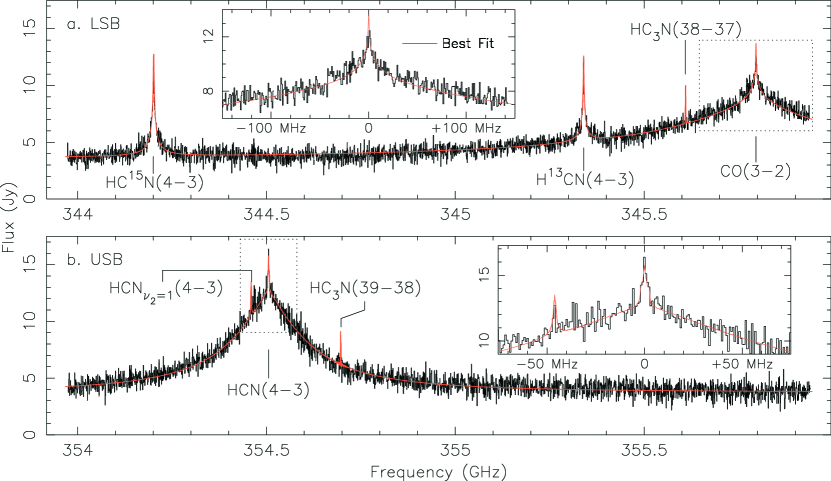
Figure 1.— Submillimeter whole-disk spectrum of Titan obtained with the SMA, with an overlayed best fit model spectrum. (a) Lower sideband containing CO(3-2), H¹³CN(4-3), HC¹⁵N(4-3), and HC₃N(38-37) rotational transitions. (b) Upper sideband with both the ground and vibrationally excited HCN(4-3) $\nu_{2}=0,1$ transitions, and the HC₃N(39-38) transition.

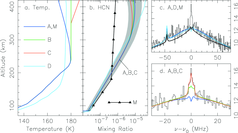
Figure 2.— (a) Model temperature profiles used in inversion analysis. (b) HCN best fit profile solutions assuming temperature models A, B, C, and D, and the HCN profile (M) determined by Marten et al. (2002). Grey scale represents the error envelope for solutions A, B, and C. (c) Observed and best fit HCN line center spectra for HCN profiles A, D, and M. (d) Observed and best fit HCN line core spectra for HCN profiles A, B, C.

References

- (1)
- (2) Courtin, R. 1988, Icarus 75, 245
- (3)
- (4) Coustenis, A., & Bézard, B. 1995, Icarus 115, 126
- (5)
- (6) Coustensis, A., et al. 2003, Icarus 161, 383
- (7)
- (8) Fegley, B. 1995, in Global Earth Physics: A Handbook of Physical Constants, ed. T.J. Ahrens (Washington, D.C.:AGU)
- (9)
- (10) Geballe, T.R., Kim, S.J., Noll, K.S., & Griffith, C.A. 2003, ApJ583, L39
- (11)
- (12) Gurwell, M.A., & Muhleman, D.O. 1995, Icarus 117, 375
- (13)
- (14) Gurwell, M.A., & Muhleman, D.O. 2000, Icarus 145, 653
- (15)
- (16) Hidayat, T., et al. 1997, Icarus 126, 170
- (17)
- (18) Hidayat, T., et al. 1998, Icarus 133, 109
- (19)
- (20) Hubbard, W.B., et al. 1993, A&A 269, 541
- (21)
- (22) Lara, L.M., et al. 1996, J. Geophys. Res. 101, 23261
- (23)
- (24) Lebonnois, S., et al. 2001, Icarus 152, 384
- (25)
- (26) Lebonnois, S., et al. 2003, Icarus 163, 164
- (27)
- (28) Lellouch, E. 1990, Ann. Geophys. 8, 653
- (29)
- (30) Lellouch, E., Romani, P.N., & Rosenqvist, J. 1994, Icarus 108, 112
- (31)
- (32) Lellouch, E., et al. 2003, Icarus 162, 125
- (33)
- (34) Lindal, G.F., et al. 1983, Icarus 53, 348
- (35)
- (36) Lutz, B.L., de Bergh, C., & Owen, T. 1983, Science 220, 1374
- (37)
- (38) Marten, A., et al. 1988, Icarus 76, 558
- (39)
- (40) Marten, A., et al. 2002, Icarus 158, 532
- (41)
- (42) Muhleman, D.O., Berge, G.L., & Clancy, R.T. 1984, Science 223, 393
- (43)
- (44) Noll, K., et al. 1996, Icarus 124, 625
- (45)
- (46) Smith, G.R. et al. 1983, J. Geophys. Res.87, 1351
- (47)
- (48) Tanguy, L., et al. 1990, Icarus 85, 43
- (49)
- (50) Toublanc, D. et al. 1995, Icarus, 113, 2
- (51)
- (52) Yelle, R.V. et al. 1997, in Huygens Science, Payload, and Mission, ESA SP, Vol. 1177 (Noordwijk, the Netherlands:Estec Publications Division, ESTEC)
- (53)
- (54) Yelle, R.V. & Griffith, C.A. 2003, Icarus 166, 107
- (55)
- (56) Yung, Y.L., Allen, M., & Pinto, J.P. 1984, ApJS 55, 465
- (57)