Emissione di alta energia da galassie starburst
(High energy emission from starburst galaxies)

Preface

The star formation (SF) can be regarded as an engine powering the light emission of spiral galaxies at several wavelengths. Massive, young stars emit the bulk of their light in the UV band; a large fraction of the UV radiation is absorbed by cold ($T\sim 40$K) dust and reradiated in the far infrared band. Massive stars explode as supernovae, and supernova remnants accelerate the electrons which in turn power the radio emission through the synchrotron mechanism. Binary systems composed by a collapsed star with a massive companion, emit X-rays through Comptonization of thermal photons coming from the accretion disc.

The star formation activity may go on for very long times at low paces, or be significantly enhanced for short times as conquence of perturbations in the gravity potential, which trigger the collapse of gas clouds. Mergers, or cannibalization of small galaxies, are often the reason for episodes of enhanced star formation.

The intensity of an episode of star formation can be classified on the basis of its sustainability for long times. If we define the Star Formation Rate (SFR, usually expressed in $M_{\odot}/$yr) as the mass of gas converted into stars per unit time, we may also consider the depletion time $\tau_{\rm d}=M_{\rm gas}/$SFR which measures the time needed to convert into stars all the mass $M_{\rm gas}$ of gas present in a galaxy if the star formation continues at a constant rate. If the depletion time is very short (much shorter than, say, a Hubble time) we may call the present SF episode a starburst episode. The galaxies with an undergoing starburst episode can be called starburst galaxies. Note, however, that in the literature the term “starburst galaxy” is also found to be loosely referred to large galaxies with quiescent SF but large SFR values.

The star formation activity plays a significant role in the evolution of galaxies. The production of heavy chemical elements results both in the build up of different stellar populations and in the pollution of the insterstellar medium (ISM). Intense starburst episodes also may form bubbles of hot ionized gas, with a pressure larger than that of the surrounding cold ISM. The bubbles may be able to expand in a direction normal to the plane of the galaxy disc, eventually releasing their gas content into the intergalactic medium (IGM). Depending on the strength of gravitational potential of the galaxy, the gas may definitely escape into the IGM or fall back (a galactic fountain is then formed).

Star formation has also undergone a strong cosmological evolution, since the average density of SFR was about ten times larger at redshifts larger than 1, and has been declining since then (Lilly et al. 1996; Madau et al. 1996). Thus the study of galaxies in the local universe with a strong star formation activity may act as a guide to understand the evolution of galaxies in the early universe.

In the following, we focus on the study of ‘normal’, spiral, star forming galaxies. The term ‘normal’ will be referred to galaxies whose energy output is dominated by all the processes related with star formation and evolution, with no contribution from a possible active galactic nucleus.

The first chapter is devoted to a review of the infrared, radio and X-ray emission from star forming galaxies. In the second chapter we explore the quantitative relationships between the total X-ray, radio and infrared luminosities for a sample of 23 star forming galaxies. It is found that linear correlations hold between the luminosities in the above bands. In the third chapter we show, by analyzing a sample of 11 high redshift galaxies in the Hubble Deep Field, that the linear correlations may be extended up to $z\sim 1$. In the fourth chapter we turn to an analysis of the luminosity function and number counts of star forming galaxies; we show that the number density of normal galaxies at faint X-ray fluxes ($10^{-17}$–$10^{-15}$ erg s^-1 cm^-2) is very well defined.

The fifth chapter offers a first insight into a different aspect of galaxy evolution, i.e. whether is it possible to determine the metallicity enhancements in a starburst episode. An interesting, yet problematic, picture of metal enrichment of the interstellar matter arises from an analysis of the X-ray and near infrared spectra of M82. Finally, a summary is offered of the work here described.

Chapter 0 Light emission from star forming galaxies

Two main stellar population are usually found in spiral galaxies: one made up by old dwarf stars, and one made up by young, blue, massive stars. While the former builds the bulk of the galaxy stellar mass and of the energetic output in the optical band, the latter powers the light emission in many different bands throughout the whole energy spectrum. In the following, it will be shown how the processes of star formation and death can be invoked to explain the light emission properties of galaxies at radio, far infrared and X-ray wavelengths.

1 Infrared emission from spiral galaxies

The far infrared luminosity ($\sim 3$–300$\mu$) of a star forming galaxy is commonly interpreted as due to starlight reradiation by dust grains. The early evidence for a link between infrared emission and dust was based on several arguments (Harwit & Pacini 1975; Telesco & Harper 1980; Devereux & Young 1990):

• H ii regions are associated with knots of infrared emission;

• the far infrared luminosities may exceed the optical luminosities, consistent with the view that the FIR radiation is generated by heavily obscured star clusters;

• the high luminosity-to-mass ratios derived from the comparison of FIR luminosities and dynamical masses, consistent with the view that the obscured star clusers are composed primarily of young massive stars;

• the FIR luminosities are well correlated with masses of the molecular gas, which is the component of the interstellar medium from which stars form.

The observations made with the Infrared Astronomical Satellite (IRAS) showed that infrared emission is ubiquitous among spiral galaxies, thus reinforcing the view that the far infrared luminosity of spiral galaxies is thermal dust emission. A comparison of the H$\alpha$ and FIR luminosities in a sample of 124 galaxies (Devereux & Young 1990) showed that the mean ratio of extinction-corrected H$\alpha$ to bolometric FIR luminosity in spiral galaxies is comparable to that expected for H ii regions powered by massive stars. This led Devereux & Young (1990) to support the view that high mass stars required to ionize the hydrogen gas can easily generate the far infrared luminosities.

However, the presence of galaxies with a low level of infrared emission that is energetically comparable to the optical luminosity also led de Jong et al. (1984) to suggest later type stars as a significant dust heating source, particularly in spirals with a cool $S_{60\mu}/S_{100\mu}$ dust temperature. It was also suggested (Lonsdale-Persson & Helou 1987; de Jong & Brink 1987) that the emission at $60\mu$ and $100\mu$ measured by IRAS could be deconvolved in two components: a warm component with temperatures of 50–60K, and a cool component (the cirrus) at 10–20K. An interpretation of the two-component model which considered the warm component as radiation from dust heated by young stars, while the cool component is heated by older, late type stars, was considered as the possible explanation for a slight non-linearity of the radio/FIR correlation (Fitt et al. 1988; however, the latest studies point toward almost exact linearity, Yun et al. 2001; see Sect. 3).

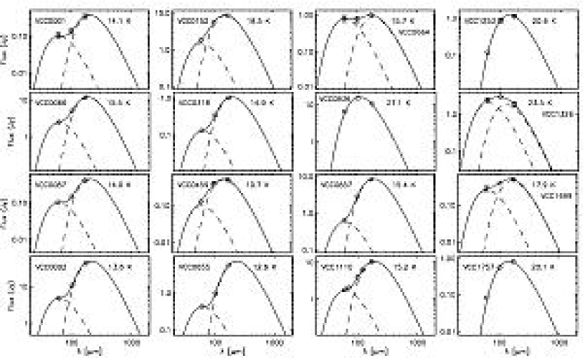
   Figure 1: Far infrared spectral energy distributions for a sample of spiral galaxies in Virgo, from Popescu et al. (2002). The points are ISOPHOT data, while the lines show the two-temperature model fit to the data (see text).

   Figure 2: Fractional contribution of ultraviolet light from different sources (H ii regions and the diffuse old stellar component) to dust heating for the spiral galaxy NGC 891, from Tuffs & Popescu (2003).

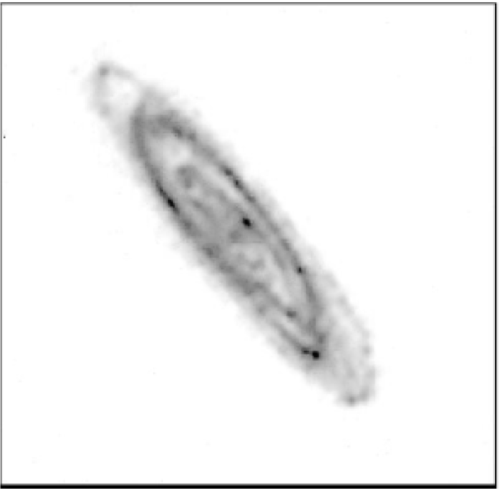
   Figure 3: ISOPHOT mapping of the M31 galaxy at 170$\mu$, from Haas et al. (1998). The darker areas show the emission due to the cold ($\sim 20$ K) dust. The angular resolution is $1.3\hbox{${}^{\prime}$}$, the field size $2.9\hbox{${}^{\circ}$}\times 2.9\hbox{${}^{\circ}$}$.

Since the peak in the thermal spectrum of dust with temperatures below $\sim 30$K falls longwards of 100$\mu$ —thus outside the IRAS bands—, a clear separation of the warm and cool components was only possible with the launch of the Infrared Space Observatory (ISO), whose spectral coverage extended up to wavelengths of $\sim 180\mu$. Popescu et al. (2002) studied a sample of 38 galaxies with the ISOPHOT instrument at 60, 100 and 170$\mu$. Most of these galaxies were discovered to contain a cold dust emission component which could not have been detected by IRAS. The FIR Spectral Energy Distributions (SEDs) of these objects were fitted with a combination of two modified blackbody functions, one physically identified with the emissions from a localised warm dust component, with a fixed temperature of 47K, and one other with a diffuse cold dust component (Figs. 2, 2). The cold dust temperatures were found to span a broad range, with a median of 18K.

Imaging of the cold component has been so far possible, with ISOPHOT, only for very extended objects such as M31 (Fig. 3). Detailed studies of the FIR emission will be routinely possible in the immediate future with the Spitzer Space Telescope. Among the first images taken with this new observatory, the pictures of M81 at different wavelengths (Plates  Emissione di alta energia da galassie starburst (High energy emission from starburst galaxies),LABEL:plate:m81longw) show the details in the spiral structure of the cold dust at 170$\mu$.

2 Radio emission

Radio sources exist in nearly all normal spiral and dwarf irregular galaxies, and in many peculiar or interacting systems. The morphology of the radio emission found in normal galaxies is various (Condon 1992, and references therein). The faintest dwarf irregulars have radio luminosities comparable with the Galactic Supernova Remnant (SNR) Cassiopea A and little or no detectable emission extending beyond known H ii regions and SNRs. Their radio morphologies are lumpy and irregular (see IC 10 in Fig. 4), and their radio spectra are often relatively flat. The thick radio disk/halo of the edge-on galaxy NGC891 and the fairly smooth radio disk with bright spiral arms of the face-on galaxy NGC6946 are typical of the larger spiral galaxies. The central radio sources in normal galaxies like NGC6946 have a larger brightness but are usually much less luminous than the disk-like sources. Luminous radio sources with complex morphologies may be found in colliding galaxies (e.g. NGC1144). There is a tendency for fairly compact (diameter $D\lesssim 1$ kpc) central starbursts to dominate at higher radio luminosities, as in M82. The most luminous radio sources in normal galaxies are frequently quite compact ($D\sim 200$ pc), and confined to the nuclei of strongly interacting systems (e.g. IC694+NGC3690). Numerical simulations show that a collision involving a disk galaxy can drive about half of the disk gas ($\lesssim 10^{10}M_{\odot}$) within 200 pc of the nucleus (Hernquist 1989; Barnes & Hernquist 1991) where the gas density becomes quite high before a powerful starburst is triggered (Kennicutt 1989). The resulting massive stars and their SNRs then produce intense radio emission.

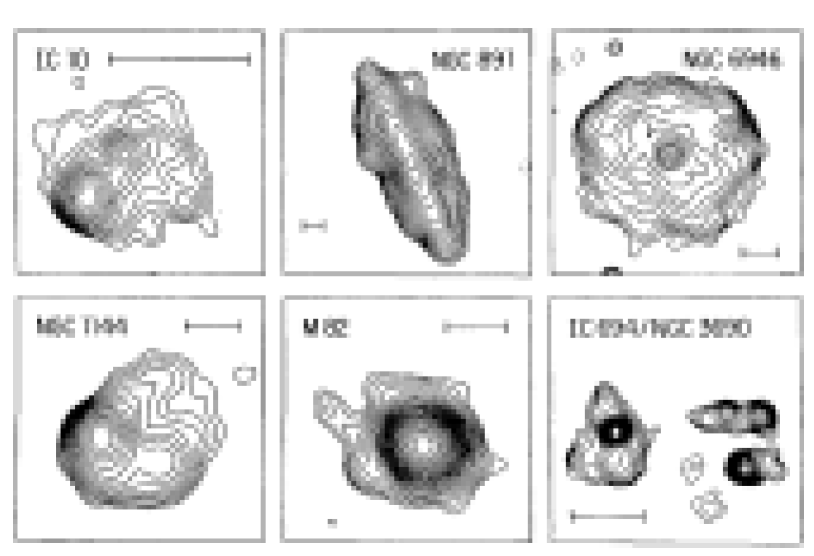
   Figure 4: Contour maps illustrating the range of radio source morphologies, sizes, and luminosities found in normal galaxies, from Condon (1992). The bars are 2$h^{-1}$ kpc long. The logarithmic contours are separated by $\sqrt{2}$ in brightness, and the 1.49 GHz brightness temperatures $T_{\rm b}$ of the lowest contours are 0.25K (IC10, NGC891, NGC6946), 0.5K (M82), 8K(NGC1144), and 128K (IC694+NGC3690).

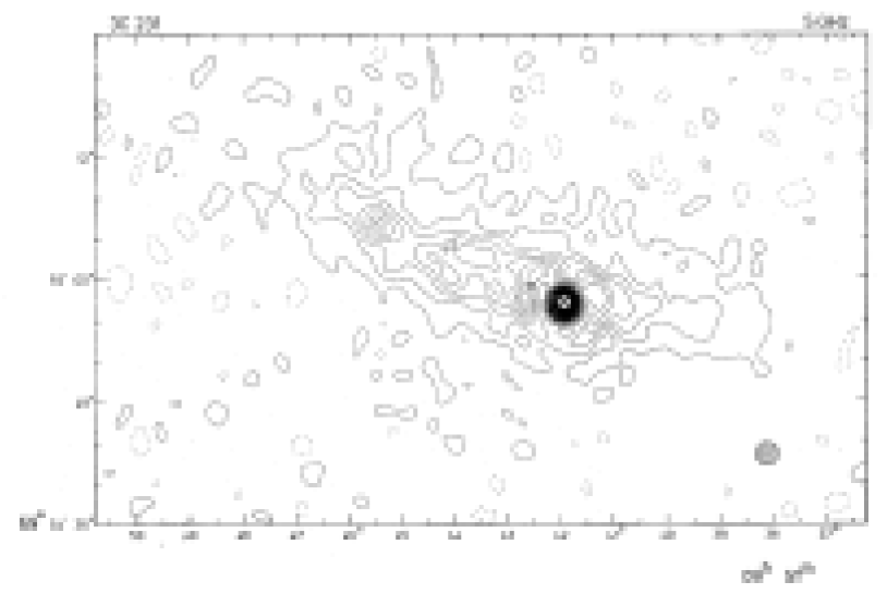
   Figure 5: Radio emission from M82. Upper panel: medium resolution image at 5GHz (Cambridge 5km radio telescope), from Hargrave (1974). Lower panel: high resolution Merlin image at 5GHz, from Muxlow et al. (1994). As normal with interferometer images, the lower the resolution, the higher the sensitivity to diffuse emission.

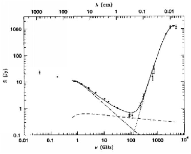
   Figure 6: Radio-FIR spectrum of M82, from Condon (1992). Dashed line: thermal contribution to the spectrum from the H ii regions. Dot-dashed line: nonthermal emission. Dotted line: black body emission from the dust. The continous line shows the fitted spectrum resulting from the sum of the previous three components.

Nearly all of the radio emission from normal galaxies is synchrotron radiation from relativistic electrons and free-free emission from H ii regions (Condon 1992). Thermal reradiation of starlight by dust quickly overwhelms these components above $\nu\sim 200$GHz, defining a practical separation between the radio and infrared bands. Typical intensities of synchrotron radiation, free-free emission, and dust reradiation are shown in the radio/FIR spectrum of M82 (Fig. 6); the radio continuum only accounts for $\lesssim 10^{-4}$ of its bolometric luminosity.

However, determining the amount of the thermal fraction is highly controversial. In principle, the relatively flat spectrum ($S(\nu)\propto\nu^{-\alpha}$ with $\alpha\lesssim 0.1$) thermal emission should be distinguishable from the steeper spectrum ($\alpha\sim 0.8$) nonthermal emission via total flux densities or maps obtained at two or more frequencies. In practice, most normal galaxies are not bright enough to be detected at frequencies much higher than $\nu\sim 10$ GHz ($\lambda\sim 3$ cm). Moreover, if integrated flux densities at only three or four frequencies are used to fit the (unknown) nonthermal spectral index and the thermal emission simultaneously, the resulting nonthermal spectral index and thermal fraction are strongly correlated. An upper limit $S_{\rm T}/S\lesssim 0.4$ to the thermal-to-total flux ratio was estimated by Klein & Emerson (1981) and Gioia et al. (1982) from the lack of a flattening of the radio spectrum in two samples of nearby spiral galaxies. The thermal fraction is highly uncertain even in the brightest and best observed galaxies such as M82 because the nonthermal component may not have a straight spectrum. By assuming a power law spectrum for M82, Klein et al. (1988) calculated a thermal flux density $S_{\rm T}=0.15$ Jy at $\nu=32$ GHz. Using practically the same data but assuming that the nonthermal spectrum steepens at high frequencies, Carlstrom & Kronberg (1991) obtained $S_{\rm T}=0.5$ Jy (and thus a thermal fraction of $\sim 70\%$, cfr. Fig. 6) at $\nu=92$ GHz, where $S_{\rm T}=0.17$ Jy (thermal fraction $\sim 25\%$) would be expected by extrapolating Klein’s estimate at 92GHz with a typical slope $\alpha=0.1$. This simple consideration shows that the estimates of the thermal fraction at high frequencies may have un uncertainty of (at least, since M82 is among the best studied galaxies) a factor of three.

Since the nonthermal spectrum has a steeper slope, the uncertainty on the thermal fraction becomes a minor issue at lower frequencies (e.g. at 1.4 GHz), where the majority of the radio emission is of nonthermal origin (cfr. Fig. 6). The nonthermal radiation is usually explained as synchrotron radiation from relativistic electrons. Only stars more massive than $\sim 8M_{\odot}$ produce the core-collapse supernovae whose remnants (SNRs) are thought to accelerate most of the relativistic electrons in normal galaxies; these stars ionize the H ii regions as well. Their lifetime is $\lesssim 3\cdot 10^{7}$ yr, while the relativistic electrons probably have lifetimes $\lesssim 10^{8}$ yr. Radio observations are therefore probes of very recent star formation activity in normal galaxies.

Supernova remnants become radio sources about 50 years after the explosion, as Rayleigh-Taylor instabilities develop in the boundary between the shock and the ambient interstellar medium, and remain visibile for hundreds or thousands of years. About 40 young SNRs are conspicuos in high resolution maps of M82 at 5 GHz (Kronberg et al. 1985; Muxlow et al. 1994, Fig. 5). Although SNRs are probably responsible for cosmic ray acceleration, discrete remnants themselves emit only a small fraction ($\lesssim 10\%$) of the integrated flux (Pooley 1969; Ilovaisky & Lequeux 1972; Biermann 1976; Helou et al. 1985). This also means that $\gtrsim 90\%$ of the nonthermal emission must be produced long after the individual supernova remnants have faded out. Most of the nonthermal emission is so smoothed by cosmic ray transport that the spatial distribution of its sources cannot be deduced in detail. Thus a various number of other possible sources for cosmic ray acceleration has been proposed, but none of them was really convincing (a review is in Condon 1992). A five-band (radio, FIR, near infrared, blue, and X-ray) study of luminosity correlations in spirals led Fabbiano et al. (1988) to conclude that the radio emission from starbursts must originate in the young stellar population but no clear conclusion can be drawn from the luminosity correlations in less active spiral galaxies.

3 The radio/FIR correlation

A correlation between the $\lambda=10\mu$ mid infrared and 1415 MHz radio luminosities of Seyfert galaxies was discovered by van der Kruit (1971) and soon extended to normal spiral galaxies (van der Kruit 1973). At first both the infrared and radio emission were thought to be synchrotron radiation from relativistic electrons accelerated by nuclear monsters (e.g. massive black holes in Seyfert galaxies or other AGN). Then Harwit & Pacini (1975) proposed that the infrared is thermal reradiation from dusty H ii regions, while the 1415 MHz is dominated by synchrotron radiation from relativistic electrons accelerated in SNRs from the same population of massive stars that heat and ionize the H ii regions. This is still the current interpretation (cfr. Sect. 1 and 2).

The real significance of the FIR/radio correlation for normal galaxies —its tightness and universality— was not appreciated until the large IRAS survey appeared (Dickey & Salpeter 1984; De Jong et al. 1985; Helou et al. 1985). The correlation has a linear slope and spans $\sim 5$ orders of magnitude in luminosity with less than 50% dispersion (Yun et al. 2001; Wunderlich et al. 1987), making it one of the tightest correlations known in astronomy (Fig. 7). It has been also tested for high redshift objects, and holds up to $z\sim 1.3$ (Garrett 2002). The correlation not only holds on global scales but is also found to hold within the disks of galaxies, down to scales of the order of a few hundreds of pc (Beck & Golla 1988).

What is most extraordinary about this relationship is that its slope is unity (the most up-to-date result gives $L_{1.4}\propto L_{60\mu}^{0.99\pm 0.01}$, Yun et al. 2001), although it couples four different radiative processes: i) thermal emission in the FIR from warm dust around H ii regions; ii) thermal emission in the FIR from cool dust (the ‘cirrus’) associated with dust heated by the old stellar population; iii) synchrotron emission at radio wavelengths; iv) thermal free-free emission at radio wavelengths.

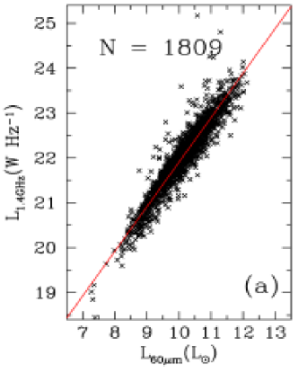
   Figure 7: The radio/FIR correlation for a sample of 1809 galaxies from the IRAS 2 Jy catalogue, from Yun et al. (2001). The correlation spans five orders of magnitude in luminosity with a best fit slope of $0.99\pm 0.01$.

Several studies have thus been devoted to investigate the correlation by focusing on one or more of these processes. Cox et al. (1988) correlated the luminosities at 60$\mu$ and 151 MHz (where the contribution of the free-free emission to the radio luminosity should be negligible) and found a non-linear slope of $L_{\rm FIR}\propto L_{151}^{0.86\pm 0.03}$. After deconvolving the FIR luminosity into two temperature components (Fitt et al. 1988), the best fits yielded $L_{\rm FIR,warm}\propto L_{151}^{0.97\pm 0.06}$ for the warm component, and $L_{\rm FIR,cool}\propto L_{151}^{\sim 0.6}$. Thus they suggested that the warm dust component was correlated with the nonthermal radio luminosity, while the link between the cool dust and the synchrotron radiation remained unexplained.

However, decoupling the warm and cool components from IRAS data alone should be taken with care, because the cool dust becomes visible only at wavelengths longer than 100$\mu$. The PHOT instrument onboard the ISO satellite was better suited for this task, because of the availability of a $170\mu$ channel. Pierini et al. (2003) thus used PHOT data taken at 60, 100 and $170\mu$ for a sample of 72 galaxies and found (note that here ‘FIR’ indicates the bolometric luminosity for the dust)

$$L_{1.4}\propto L_{\rm FIR}^{1.10\pm 0.03}\qquad L_{1.4}\propto L_{\rm FIR,warm}^{1.03\pm 0.03}\qquad L_{1.4}\propto L_{\rm FIR,cool}^{1.13\pm 0.04}$$ (1)

thus confirming the view that the warm dust and the nonthermal radio luminosity are linearly correlated. Also their best-fit slope for the cool dust/radio correlation is consistent, within the errors, with Fitt et al. (1988).

Theoretical models for the radio/FIR correlation

One of the earliest theories, the ‘optically-thick’ or ‘calorimeter’ theory (Völk 1989; Völk & Xu 1994; Lisenfeld et al. 1996), is based on three main assumptions. First, that all the far ultraviolet (i.e. $\sim 5$–13.6 eV) radiation from massive stars is absorbed by the dust grains within a galaxy. Second, that the energetic electrons produced by the supernova explosions of these stars lose most of their energy within the galaxy due to synchrotron and inverse Compton process. As both these processes are proportional to the number of massive stars, these calorimetric assumptions lead to the linear correlation. Finally, the tightness of the correlation is provided by the third assumption that the energy density of the interstellar radiation field, $U_{\rm rad}$, is in a constant ratio with the magnetic field energy density, $U_{B}$.

An alternative theory put forward by Helou & Bicay (1993) assumes the opposite extreme, an ‘optically-thin’ model, in which the cosmic rays and UV photons both have high escape probabilities. To provide the correlation in these optically- and cosmic ray thin galaxies they rely on the assumptions that the UV or dust heating photons and the radio emitting cosmic rays are created in constant proportion to each other, which is again related to star formation. Then, to obtain a linear correlation, it is required by the theory that the magnetic field strength and the gas density are coupled.

A challenge to both these theories is the model by Niklas & Beck (1997). In this work they argue that observations indicate that within most galaxies, the cosmic ray electrons lose very little energy before they escape. These same galaxies are optically thick to UV photons, thus both the calorimetric and optically thin models are not supported by the observations. In the Niklas & Beck (1997) model, the controlling factor they put forward for the correlation is the gas density: they assume that both the star formation rate (and thus dust heating) and the magnetic field strength (which determines the synchrotron emission) are correlated with the gas volume density.

All these models require a sort of fine tuning between the magnetic field strength and another parameter (the radiation field or the gas density). As a way out from the fine tuning hypoteses, two mechanisms have been proposed. Bressan et al. (2002) suggested that, in a ‘calorimeter’ theory, the radio/FIR correlation may arise if the SFR remains contant for a time longer than the synchrotron-loss timescale. Under this hypothesis, the nonthermal radio luminosity of a galaxy is proportional to the integral of the synchrotron power over the electron lifetime, and an increase of the former in a larger magnetic field is compensated by a shortening of the latter.

Another mechanism was proposed by Groves et al. (2003). Following the Niklas & Beck (1997) model, Groves et al. (2003) proposed magneto-hydrodynamic turbulence as a possible mechanism to provide coupling between the gas density and the magnetic field strength, under the requirement that the radio and FIR emission is produced in the same volume element.

A ‘definitive’ model has not yet emerged. Further work is needed, as the current models do not explain the (non-linear) correlation between the radio emission and the cool dust emission. Also, the possibility that both the FIR and radio emission increase more than linearly with increasing SFR has been invoked (Bell 2003). Possible reasons might be that low luminosity galaxies have significantly less dust absorption (hence their infrared emission misses most of the star formation), and that the thermal fraction of radio emission increases with the SFR. Thus the radio/FIR correlation would arise as a sort of conspiracy.

   Figure 8: A comparison of SFR estimates from radio, infrared, H$\alpha$ and ultraviolet emission, from Cram et al. (1998). The radio/FIR correlation (upper panel) has the least scatter.

4 SFR indicators

Here we will present some very simple considerations, on which the models reviewed in Sect. 3 are based, on how to link the luminosity and the star formation rate. If we assume that the dust surrounding the SF region is optically thick to the UV radiation emitted by young stars, and there is no other process leading to far infrared emission, we may write

$$L_{\rm FIR}\propto\int_{M_{\mathrm{l}}}^{M_{\mathrm{u}}}k\Psi(M)\,\tau(M)\,L(M)\,{\rm d}M$$ (2)

where $\Psi(M)$ is the (time independent) Initial Mass Function (IMF), i.e. the probability that a star of mass $M$ is formed in an episode of SF, $k$ is a normalization for the IMF giving the actual number of stars formed per unit time, and $\tau(M)$ and $L(M)$ are the lifetime and UV luminosity of a star with mass $M$, respectively. Under the hypothesis of continous star formation, or if a burst is long enough to reach a steady state in the mass distribution of stars, then $k\Psi(M)\tau(M)$ is the number of stars with mass $M$ actually present. $M_{\rm l}$ may be taken as the lowest possible mass for a star which emits most of its luminosity in the UV band ($6M_{\odot}$, Devereux & Young 1990; however in the following the SFR calibrations will be given for $M_{\rm l}=5M_{\odot}$). $M_{\rm u}$ is upper bound of the IMF; it is usually assumed $M_{\rm u}=100M_{\odot}$ or $120M_{\odot}$, however for a Salpeter IMF ($\Psi(M)\propto M^{-2.35}$) the integral is not really dependent on this parameter. The life time for a main sequence star may be written as

$$\tau\propto\frac{qMX}{L}$$ (3)

where $q$ is the hydrogen fraction actually burned, and $X$ is the hydrogen abundance. Thus $L(M)\tau(M)\propto M$. Since we define

$$\mathrm{SFR}\,(M>M_{\mathrm{i}})=\int_{M_{\mathrm{i}}}^{M_{\mathrm{u}}}\,M\,k\Psi(M)\,dM$$ (4)

then we get that $L_{\rm FIR}\propto\,$SFR.

Thus we may take (Cram et al. 1998)

$${\rm SFR}_{60\mu}(M>5M_{\odot})=2.0\cdot 10^{-31}L_{60\mu}$$ (5)

with $L_{60\mu}$ in erg s^-1 Hz^-1. Another calibration (Kennicutt 1998; Cram et al. 1998)

$$\mathrm{SFR}_{FIR}(M>5M_{\odot})=4.5\cdot 10^{-44}L_{\mathrm{FIR}}\quad M_{\odot}\,\mathrm{yr}^{-1}$$ (6)

makes use of the $FIR$ parameter(Helou et al. 1985)

$$FIR=1.26\cdot 10^{-11}(2.58S_{60\mu}+S_{100\mu})\quad\mathrm{erg}\,\mathrm{s}^{-1}\,\mathrm{cm}^{-2}$$ (7)

with $S_{60\mu}$ and $S_{100\mu}$ in Jy. The $FIR$ parameter estimates the flux which would be measured by a theoretical detector with flat response between 42.5$\mu$ and 122.5$\mu$ if the underlying spectrum is a modified black body law

$$B(\nu,T)=\frac{2h\nu^{3}}{c^{2}}\frac{1}{e^{\frac{h\nu}{kT}}-1}\left(1-e^{-\left(\frac{\nu}{\nu_{0}}\right)^{\beta}}\right)$$ (8)

with $20{\rm K}\lesssim T\lesssim 80$K and $0\lesssim\beta\lesssim 2$.

If, on the other hand, we assumed that the dust and gas are optically thin for the emission in the ultraviolet band and the H$\alpha$ line, a similar reasoning might have been made by changing $L_{\rm FIR}$ with $L_{\rm UV}$ or $L_{{\rm H}\alpha}$ in Eq. (2). Balmer line emission from star-forming galaxies is formed in H ii regions ionized by early-type stars. Kennicutt (1983) has determined the theoretical relationship between the H$\alpha$ luminosity and the current rate of star formation in a galaxy in a form corresponding to

$${\rm SFR}_{{\rm H}\alpha}(M>5M_{\odot})=\frac{L_{\mathrm{H}\alpha}}{1.5\cdot 10^{41}\ \rm erg\ s^{-1}}\quad M_{\odot}\,\mathrm{yr}^{-1}.$$ (9)

The use of far-UV or U-band luminosities to infer the current SFR rests on the idea that UV emission contains a substantial contribution of light from the photospheres of young, massive stars (Cowie et al. 1997). However, the calibration of a UV indicator is less straightforward than those listed above, because of the large numbers of relatively old stars that also contribute to the actual U-band luminosity of disk galaxies. To avoid this problem, Cram et al. (1998) used the relationship between SFR and far-UV luminosity given by Cowie et al. (1997), scaled from 250 nm to the U-band using relevant synthesized spectra, to derive

$${\rm SFR}_{\rm UV}(M>5M_{\odot})=\frac{L_{\rm UV}}{1.5\cdot 10^{29}\ \rm erg\ s^{-1}}\quad M_{\odot}\,\mathrm{yr}^{-1}.$$ (10)

The two hypotheses made above (the dust and gas being optically thick or thin to UV radiation) are obviously at odds. Here we will not venture into details, but rather remind that in a patchy distribution of dust/gas clouds (a “leaky cloud” model, Devereux & Young 1990; Boulanger & Perault 1988), a fraction of the ultraviolet/H$\alpha$ radiation produced in an H ii region may still be able to escape. Clearly, extinction corrections will be needed to recover the SFR from UV/H$\alpha$ observations. SFR estimates from UV and H$\alpha$ vs. radio are shown in Fig. (8), middle and lower panel respectively. If we assume that the radio luminosity is a good SFR indicator (see next paragraph), then the high scatter and the non-linearity of the (UV, H$\alpha$)-radio relation cleary shows the effects of extinction. Note that Eq. (9) incorporates a correction for the average extinction suffered in spiral galaxies (Kennicutt 1983), thus the scatter is entirely due to the individual variations of the amount of absorption in individual galaxies.

The radio emission may be linked to the SFR with similar arguments (Condon 1992). If all stars with mass $M\geq M_{\rm sn}$ end their life as core-collapse supernovae, then the supernova rate may be defined as

$$\nu_{\rm SN}=\int_{M_{\rm SN}}^{M_{\rm u}}k\Psi(M)\,{\rm d}M$$ (11)

and, assuming that SNR are radio sources only during their adiabatic lifetime, the nonthermal luminosity might be written as

$$L_{\rm NT}\propto E^{-1/17}n^{-2/17}\nu_{\rm SN}.$$ (12)

where $E$ is the supernova explosion energy, and $n$ is the ambient particle density. However, it is impossible to reconcile the supernova rates needed by Eq. (12) with those observed in galaxies, since the former are about ten times larger. Thus it was proposed (Pooley 1969; Ilovaisky & Lequeux 1972) that SNRs may accelerate the relativistic electrons producing the nonthermal radio emission, but $\gtrsim 90\%$ of this emission must be produced long after the individual supernova remnants have faded out and the electrons have diffused throughout the galaxy. Thus it may be better to use the empirical relation observed in the Milky Way

$$L_{\rm NT}\sim 13\,\nu^{-\alpha}\,\nu_{\rm SN}$$ (13)

whit $L_{\rm NT}$ in units of $10^{29}$ erg/s, $\nu$ in GHz and $\nu_{\rm SN}$ in yr^-1; the average $\alpha$ found in spiral galaxies is $\sim 0.75$ (Condon 1992). Eq. (13) probably applies to most normal galaxies, since significant variations in the ratio $L_{\rm NT}/\nu_{\rm SN}$ would violate the observed radio/FIR correlation. Also, Völk et al. (1989) argued that the cosmic ray energy production per supernova is the same in M82 as in the Galaxy. Thus we have, in terms of the SFR:

$$L_{\rm NT}\sim 5.3\cdot 10^{28}\nu^{-\alpha}SFR.$$ (14)

5 X-ray emission: the Chandra and XMM-Newton revolution

It has been known since the late eighties that star forming galaxies are luminous sources of X-ray emission, due to a number of X-ray binaries, young supernova remnants, and hot plasma associated to star forming regions and galactic winds (Fabbiano 1989). The X-ray emission is a key tool in understanding the star formation processes, since it traces the most energetic phenomena (mass accretion, supernova explosions, gas heating, cosmic rays acceleration), and it is a probe into the dense and dusty star forming regions.

In the last few years —i.e. after the launch of Chandra and XMM-Newton—, the ‘common picture’ of normal galaxies underwent a dramatic review, thanks to the quantum leap in sensitivity, angular and spectral resolution achieved by the new observatories (cfr. Table 1). As an example, in LABEL:plate:antennaeX-raya the images of the Antennae galaxy (NGC3038/9) taken with ROSAT and ASCA are shown beside an optical image from the Digitized Sky Survey. The improvement provided by Chandra (LABEL:plate:antennaeX-rayb) is striking, since it provides a ten-fold increase in angular resolution with respect to ROSAT, while still offering a spectral resolution comparable to ASCA.

Telescope	PSF	Effective area	Spectral resolution	Bandpass
(instrument)	(FWHM)	(cm-2 at 1 keV)	($E/\Delta E$ at 1 keV)	(keV)
Einstein (IPC)	$60\hbox{${}^{\prime\prime}$}$	100	0.7	0.4-3.5
ROSAT (PSPC-B)	$25\hbox{${}^{\prime\prime}$}$	200	2.5	0.1–2.4
ROSAT (HRI)	$3\hbox{${}^{\prime\prime}$}$	80	—	0.1–2.4
ASCA⋆	$50\hbox{${}^{\prime\prime}$}$	420	10	0.5–10
BeppoSAX†	$90\hbox{${}^{\prime\prime}$}$	60	5	0.1–300
Chandra (ACIS)	$0.5\hbox{${}^{\prime\prime}$}$	350	10	0.5–8
XMM-Newton (EPIC)‡	$6\hbox{${}^{\prime\prime}$}$	1500	13	0.5–10
XMM-Newton (RGS)	($\sim 15\hbox{${}^{\prime\prime}$}$)	100	300	0.3–2.0

   Table 1: Characteristics of past and current X-ray telescopes. ^⋆effective area: GIS+SIS; energy resolution: SIS. ^†effective area: LECS; PSF: MECS. ^‡effective area: MOS+PN; energy resolution: MOS.

Point sources (X-ray binaries and young SNRs) have emerged as the dominant contributors to the overall X-ray emission, especially in the hard band (i.e. 2.0–10 keV); diffuse emission is nonetheless significant in the soft band (0.5–2.0 keV) for the galaxies with the largest SFRs, such as M82 (Griffiths et al. 2000) where the diffuse emission accounts for $\sim 30\%$ of the soft emission. In the following, the main characteristics of the different kinds of sources will be briefly discussed.

X-ray binaries are the brightest class of point sources in galaxies (reviews may be found in White et al. 1995; van Paradijs 1998; Persic & Rephaeli 2002); they are formed by a collapsed star (black hole or neutron star) with a normal companion (main sequence or giant). Although the properties of their X-ray emission (luminosity, variability, spectrum, whether the emission is persistent or transient) depend on a number of parameters (mainly the masses of the two stars and the accretion rate), an essentially full characterization of X-ray binaries can be made on the basis of the mass of the donor star. We have High Mass X-ray Binaries (HMXB) when the donor is a main sequence star with $M\gtrsim 8M_{\odot}$, and Low Mass X-ray Binaries (LMXB) when the donor is a post main sequence star with $M\lesssim 1M_{\odot}$ (binary systems with intermediate mass donor stars turn out not to be effective X-ray emitters). This main distinction has to do with the nature of the mass transer — wind accretion in HMXB, transfer via Roche-lobe overflow in LMXB.

The spectral shape of X-ray binaries may be basically seen as the sum of two components: a black body with $kT\gtrsim 1$ keV (‘soft component’, associated with an accretion disc) and a power law $S(E)\propto E^{1-\Gamma}$ with slope $\Gamma\sim 1.2$ for the HMXB and $\sim 1.4$ for the LMXB (‘hard component’, arising from Comptonization of the photons form the accretion disc); the relative weight of the two components may vary with time, and one of the components may even completely dominate the overall emission — a transition occurs between the so-called soft (or high) and hard (or low) states (cfr. Sect. 6). The overall X-ray luminosity is usually comprised in the $10^{37}$–$10^{39}$ erg/s interval, with the HMXBs somewhat brighter on average, and depends for both types on how close the normal star is to fill its Roche lobe: the closer, the brighter.

Supernova remnants are moderately luminous sources ($L_{\rm X}\sim 10^{37}$ erg/s) in the early part of their life, namely during the free expansion phase and the beginning of the adiabatic expansion phase (Woltjer 1972; Chevalier 1977). Their spectrum can be described as a thermal plasma with decreasing temperature, from $kT\sim 40$ to $\sim 0.4$ keV in about $10^{3}$ yr, as the remnant expands (assuming a rather dense ISM as should be the case in the most actively star forming galaxies; namely $n\sim 10^{3}$ cm^-3, following Chevalier & Fransson 2001; see also Draine & Woods 1991). This rather short lifetime makes SNRs a minor component among X-ray sources in galaxies, accounting for $\lesssim 10\%$ of the total number of point sources (Pence et al. 2001; Persic & Rephaeli 2002). It is nonetheless interesting to note that since the radio-emitting phase only begins $10^{4}$ yr after the supernova explosion, X-ray and radio SNRs represent two different evolutive phases of the same population of objects; indeed the comparison of Chandra and radio images has shown that sources emitting in both bands are very rare (Chevalier & Fransson 2001).

The interstellar medium (ISM) itself, when heated by supernova explosions, turns into an X-ray source. Soft, diffuse emission in galaxies was already observed with Einstein, and at least one thermal component with a temperature around $\sim 1$ keV was required to fit the ASCA and BeppoSAX data (Ptak et al. 1997; Cappi et al. 1999). Its spectrum may be described as a Bremsstrahlung component plus a number of atomic recombination lines. Depending on the ISM density, the SFR, and the gravity potential of the galaxy, the hot high-pressure plasma may eventually find a way out of the galaxy disc and escape into the intergalactic medium — thus creating an outflow (LABEL:plate:M82chandra). Observations conducted with the ROSAT HRI instrument showed a spatial overlap of the X-ray emission with H$\alpha$ emission from the outflow (Della Ceca et al. 1996, 1997). It was not clear, however, if the X-ray emission came from the interface between the ambient material and the wind, or from the wind itself. Chandra observations showed that the X-ray emission has a conical, shell-like shape (LABEL:plate:NGC253xmmchandrab; Strickland et al. 2000). It can be explained as the hot rarefied and expanding wind heats the surrounding material which in turn produces the X-ray emission. XMM-Newton observations (LABEL:plate:NGC253xmmchandraa) have shown that also the galactic disc is an X-ray emitter. An interesting and yet unresolved question is the fate of the metals produced in the supernova explosions: whether they mix with the ISM or escape from the galaxy; cfr. Chap. 4.

   Figure 9: X-ray spectrum of M82. Upper panel: observed data from the pn instrument onboard XMM-Newton, rebinned to achieve a significance of at least $15\sigma$ per energy bin. The continous line shows the model, folded with the instrumental response. Lower panel: model spectrum (continous line) composed by a hot plasma (dashed line) plus an absorbed power law (dot-dashed line).

The total spectrum of a star forming galaxy is thus made up by the sum of a thermal spectrum from hot plasma and of a power law representing the emission from the X-ray binaries. While a detailed discussion of the relative contribution of the different classes of sources to the total spectrum may be found in Persic & Rephaeli (2002), we will focus here on two simple considerations: i) the power law component is often found to be absorbed, with column densities aroud $10^{21-22}$ cm^-2 (Ptak et al. 1999; Moran et al. 1999); ii) the thermal component has a steeper slope than the power law. The joint effect of the steeper slope of the thermal component, and of absorption on the power law, makes the two components mainly emit in different energy bands: the plasma dominates at softer energies ($\lesssim 1$–2 keV) and the binaries at harder ones. As an example, the spectrum of the galaxy M82 obtained with the pn instrument onboard XMM-Newton is shown in Fig. (9). It is interesting to notice that, although the individual spectrum of X-ray binaries has a slope around $\Gamma\sim 1.2$–1.4, the resulting total spectrum of a galaxy may have a flatter slope if a number of binaries is present with different absorbing column densities; cfr. the Chandra spectrum of the point sources in M82, Fig. 3. Conversely, if the spectrum of the X-ray binaries is not heavily absorbed, the more intense the plasma emission, the more steep the overall spectrum of a galaxy. As a consequence, a relatively large spread may be found in the average hard X-ray spectrum of starburst galaxies (Ptak et al. 1999).

An active galactic nucleus (AGN) may also be present in star forming galaxies. While it has been proposed that nuclear activity might be related to enhanced star formation (the ‘starburst/AGN connection’) as a consequence of the disposal of large quantities of gas, nuclear activity is not truly a star formation related process. If present, moreover, an AGN tends to dominate over the X-ray emission from the rest of the galaxy. A typical AGN luminosity ($L_{\rm X}\gtrsim 10^{42}$ erg/s) exceeds by (at least) a few orders of magnitude the emission from a normal galaxy ($L_{\rm X}\sim 10^{40\pm 1}$ erg/s). Thus the main concern about AGN in X-ray studies of starburst galaxies has been so far to exclude them from the galaxy samples (cfr. Sect. 1). The high resolution of Chandra allows to resolve most nearby galaxies, so that AGN may be identified and properly accounted for in data analysis (Ho et al. 2001). However, the problem still arises for more distant, hence unresolved, galaxies.

Optical spectroscopy is the main tool used in the classification of Seyfert vs. star forming galaxies. The equivalent widths of emission lines from the centre of a galaxy are used in diagnostic diagrams to determine the excitation and ionization states of the nebular gas, which in turn are determined by the nature of the energy source (Veilleux & Osterbrock 1987). Although a determination of the X-ray luminosity and/or an optical spectrum usually suffice, this can prove to be a difficult task, especially for luminous dusty objects (such as NGC 3256, NGC 3690, NGC 6240, Arp220) in which the overall luminosity is still sustainable by star formation, and AGN signatures may be hidden by absorption. NGC 3690 (Della Ceca et al. 2002) and NGC 6240 (Vignati et al. 1999) are emblematic cases: both of them are currently undergoing a powerful starburst (100–200 $M_{\odot}$/yr), and the optical spectrum does not show clear AGN signatures; however when observed with the PDS instrument onboard BeppoSAX they have shown the emergence at energies larger than 10 keV of a heavily absorbed ($N_{\rm H}\sim 10^{24}$ cm^-2) nuclear component.

At high redshifts ($z\sim 1$), the use the diagnostic diagrams in separating Seyfert galaxies from star forming ones has to be treated with caution because of two effects: a possibly lower signal/noise ratio, and the shift of emission lines outside the observing spectral band. Moreover, because of the little angular size (a few arcsec) of high redshift galaxies, it is not possible to obtain a spectrum of the central regions only. Thus the signatures of a low luminosity AGN may be diluted in the overall radiation of the galaxy. With this caveat, optical spectroscopy may still be regarded as an effective method in selecting candidate star forming galaxies at high redshifts.

Chapter 1 The X-ray luminosity as a SFR indicator

While radio continuum and far infrared (FIR) luminosities of star-forming galaxies are known to show a tight linear relationship spanning four orders of magnitude in luminosity and up to a redshift $\sim 1.3$ (Sect. 3), a relation between FIR and X-ray luminosities was found in the early nineties but its details remained somewhat controversial. A non linear ($L_{\rm X}\propto L_{\rm FIR}^{0.6}$) and highly scattered (dispersion of about 2 dex) relation was found between FIR and soft (0.5–3.0 keV) X-ray luminosities of IRAS-bright and/or interacting/peculiar galaxies measured by the Einstein satellite (Griffiths & Padovani 1990). A somewhat different result was found by David et al. (1992), i.e. a linear relation between FIR and 0.5–4.5 keV luminosities for a sample of starburst galaxies observed by Einstein. A large number of upper limits to the X-ray flux (12 upper limits vs. 11 detections for Griffiths & Padovani 1990) along with high uncertainties in the X-ray and FIR fluxes may explain this discrepancy. Moreover, these studies suffered by the lack of knowledge about spectral shapes and internal absorption in star forming galaxies caused by the limited sensitivity and spectral capabilities of the IPC detector onboard Einstein.

In this chapter, with the high sensitivity and the broad-band spectral capabilities of the ASCA and BeppoSAX satellites, we extend these studies to the 2–10 keV band which is essentially free from absorption. In the following paragraphs a sample of nearby star forming galaxies is assembled (Sect. 1) and linear relations among radio, FIR and both soft and hard X-ray luminosities are found (Sect. 2). Possible biases are discussed and the use of X-ray luminosities as a SFR indicator is proposed (Sect. 3). In Chap. 2 we present a study of star-forming galaxies in the Hubble Deep Field North and test the validity of the X-ray SFR law. Implications for the contribution of star-forming galaxies to the X-ray counts and background are discussed in Chap. 3.

Throughout this thesis we assume, unless otherwise stated, $H_{0}=70$, $\Omega_{\rm M}=0.3$ and $\Omega_{\Lambda}=0.7$.

1 The local sample

The atlas of optical nuclear spectra by Ho et al. (1997) (hereafter HFS97) represents a complete spectroscopic survey of galaxies in the Revised Shapley-Ames Catalog of Bright Galaxies (RSA; Sandage & Tammann 1981) and in the Second Reference Catalogue of bright galaxies (RC2; de Vaucouleurs et al. 1976) with declination $\delta>0\hbox{${}^{\circ}$}$ and magnitude $B_{T}<12.5$. Optical spectra are classified in HFS97 on the basis of line intensity ratios according to Veilleux & Osterbrock (1987); galaxies with nuclear line ratios typical of star-forming systems are labeled as “H ii nuclei”. This sample of H ii galaxies contains only spirals and irregulars from Sa to later types, except for a few S0 which were excluded from our analysis since their properties resemble more those of elliptical galaxies.

A cross-correlation of the HFS97 sample with the ASCA archive gives 18 galaxies clearly detected in the 2–10 keV band with the GIS instruments. Since most of these galaxies were observed in pointed observations (rather than in flux-limited surveys) it is unlikely that the results hereafter shown are affected by a Malmquist bias. Four additional objects in the field of view of ASCA observations were not detected: the 2–10 keV flux upper limits are too loose to add any significant information, and thus we did not include them in the sample. The cross-correlation of the HFS97 sample with the BeppoSAX archive does not increase the number of detections. When a galaxy was observed by both satellites, the observation with better quality data was chosen.

Far infrared fluxes at 60$\mu$ and 100$\mu$ were taken from the IRAS Revised Bright Galaxy Sample (RBGS, Sanders et al. 2003) which is a reprocessing of the final IRAS archive with the latest calibrations. While the RBGS measurements should be more accurate, we checked that the use of the older catalogue of IRAS observations of large optical galaxies by Rice et al. (1988), coupled with the Faint Source Catalogue (FSC, Moshir et al. 1989) for smaller galaxies, does not significantly change our statistical analysis. FIR fluxes for NGC 4449 were taken from Rush et al. (1993). Radio (1.4 GHz) fluxes were obtained from the Condon et al. (1990, 1996) catalogues (except for NGC 4449, taken from Haynes et al. 1975). Distances were taken from Tully (1988) and corrected for the adopted cosmology.

Part of the X-ray data have already been published; in the cases where published data were not available in a form suitable for analysis, the original data were retrieved from the archive and reduced following standard procedures and with the latest available calibrations. Images and spectra were extracted from the pipeline-screened event files. The images were checked against optical (Digital Sky Survey) and, where available, radio (1.4 GHz) images in order to look for possible source confusions. Fluxes were calculated in the 0.5–2.0 and 2–10 keV bands from best-fit spectra for the GIS2 and GIS3 instruments and corrected for Galactic absorption only. The uncertainty on the fluxes is of the order of 10$\%$. Depending on the quality of data, the best-fit spectrum is usually represented by a two-component model with a thermal plasma plus a power-law or just a power-law.

The galaxies IC 342 and M82 have shown some variability, mainly due to ultraluminous X-ray binaries. For the two of them we summarize in Sect. 6 the results from several X-ray observations and estimate time-averaged luminosities.

One object (M33) was not included in the sample since its broad-band (0.5–10 keV) X-ray nuclear spectrum is dominated by a strong variable source (M33 X-8) identified as a black hole candidate (Parmar et al. 2001).

Therefore, the sample (hereafter local sample) consists of the 17 galaxies listed in Table 1. Since it is not complete in a strict sense due to the X-ray selection, we have checked for its representativeness with reference to the SFR. The median SFR value for HFS97 was computed from the FIR luminosities and resulted SFR${}_{\rm med}\sim$ 1.65 M_⊙/yr. Considering objects with SFR $>{\rm SFR}_{\rm med}$ there are 14 galaxies in the local sample out of 98 in HFS97 (14$\%$), while there are 3 objects with SFR $<{\rm SFR}_{\rm med}$ (3$\%$). Thus the high luminosity tail is better sampled than the low luminosity one.

We also include data for 6 other well-known starburst galaxies which were not in the HFS97 survey because they are in the southern emisphere. On the basis of their line intensity ratios they should be classified as H ii nuclei. In Table 1 we label them as supplementary sample.

Fluxes and Luminosities: Main Sample
Galaxy	$D$	$F_{0.5-2}$	$L_{0.5-2}$	$F_{2-10}$	$L_{2-10}$	$F_{\rm FIR}$	$L_{\rm FIR}$	$F_{1.4}$	$L_{1.4}$	Refs.
M82*	5.6	97	3.6	290	11	67	25	7.7	2.9	1
M101	5.7	5.4	0.22	6.8	0.27	6.0	2.4	0.75	0.30	this work
M108	15	4.4	1.2	6.0	1.6	2.0	5.4	0.31	0.83	this work
NGC891	10	8.3	0.99	19	2.3	4.5	5.4	0.70	0.84	this work
NGC1569	1.7	5.4	0.019	2.2	0.0077	2.5	0.088	0.41	0.014	2
NGC2146	18	8.2	3.4	11	4.5	7.3	30	1.1	4.5	3
NGC2276	39	2.1	3.9	4.4	8.1	0.85	16	0.28	5.2	this work
NGC2403	4.5	16	0.39	9.3	0.23	2.7	0.65	0.33	0.080	this work
NGC2903	6.7	7.9	0.43	7.0	0.38	3.7	2.0	0.41	0.22	this work
NGC3310	20	7.4	3.5	2.1	1.0	1.7	8.1	0.38	1.8	4
NGC3367	46	1.8	4.5	1.6	4.0	0.38	9.5	0.10	2.5	this work
NGC3690	49	5.7	17	11	32	5.3	150	0.66	19	4
NGC4449	3.2	8.3	0.10	4.8	0.060	1.9	0.23	0.6	0.074	5
NGC4631	7.1	9.4	0.57	9.3	0.57	4.9	3.09	1.2	0.73	6
NGC4654	18	0.6	0.2	0.9	0.3	0.93	3.5	0.12	0.46	this work
NGC6946	5.9	30	1.2	12	0.49	7.9	3.2	1.4	0.57	this work
IC342	4.2	18	0.38	110	2.3	11	2.3	2.3	0.49	this work
Supplementary Sample
NGC55	1.4	18	0.040	6.8	0.015	4.7	0.10	0.38	0.0084	6
NGC253*	3.2	25	0.31	50	0.62	49	6.1	5.6	0.69	1
NGC1672	16	5.8	1.7	6.1	1.8	2.3	6.8	0.45	1.3	this work
NGC1808	11	6.5	1.0	7.6	1.2	5.3	8.2	0.52	0.81	this work
NGC3256	40	9.0	17	6.2	12	4.8	92	0.66	13	7
Antennae	27	7.2	6.3	5.3	4.7	2.6	23	0.57	5.0	8

   Table 1: Data for galaxies in our local samples. All galaxies were observed with ASCA, except those marked with * observed by BeppoSAX. Distances in Mpc; X-ray fluxes in $10^{-13}$ erg s^-1 cm^-2, FIR fluxes in $10^{-9}$ erg s^-1 cm^-2 and radio fluxes in Jy; X-ray luminosities in $10^{40}$ erg s^-1, FIR luminosities in $10^{43}$ erg s^-1 and radio luminosities in $10^{29}$ erg s^-1 Hz^-1. The uncertainty on fluxes and luminosities is of the order of 10$\%$.
References: 1 Cappi et al. (1999); 2 Della Ceca et al. (1996); 3 Della Ceca et al. (1999); 4 Zezas et al. (1998); 5 Della Ceca et al. (1997); 6 Dahlem et al. (1998); 7 Moran et al. (1999); 8 Sansom et al. (1996).

2 The radio/FIR/X-rays correlation

As a preliminary test, we perform a least-squares analysis for the well-known radio/FIR correlation, which yields

$$\mbox{Log}(L_{\rm FIR})=(0.98\pm 0.06)~{}\mbox{Log}(L_{\rm 1.4})+15.4\pm 1.6$$ (1)

The dispersion around the best-fit relation is given as the estimate $s$ of the standard deviation $\sigma$:

$$s=\frac{1}{N-\nu}\cdot\sqrt{\sum\left(\mbox{Log}~{}L_{\rm obs}-\mbox{Log}~{}L_{\rm pred}\right)^{2}}$$ (2)

where $\nu$ is the number of free parameters and $N$ is the number of points in the fit), $L_{\rm pred}$ is the luminosity expected from the best fit relation and $L_{\rm obs}$ the observed one. For the radio/FIR correlation (Eq. 1) we find $s=0.18$.

Following Helou et al. (1985) we also calculate the mean ratio $q$ between the logarithms of FIR and radio fluxes, obtaining $q\sim 2.2\pm 0.2$. This value is consistent with the mean $q=2.34\pm 0.01$ for the 1809 galaxies in the IRAS 2 Jy sample by Yun et al. (2001).

Soft X-rays

A test for the soft X-ray/FIR/radio relations (Fig. 1) yields

$$\mbox{Log}(L_{0.5-2}) = (0.87\pm 0.08)~{}\mbox{Log}(L_{\rm FIR})+2.0\pm 3.7$$ (3)

$$\mbox{Log}(L_{0.5-2}) = (0.88\pm 0.08)~{}\mbox{Log}(L_{\rm 1.4})+14.6\pm 2.2\vskip 6.0pt plus 2.0pt minus 2.0pt$$ (4)

with $s\sim 0.26$ and 0.24 respectively.

Our result is consistent with the $L_{0.5-4.5}\propto L_{\rm FIR}^{0.95\pm 0.06}$ relation found by David et al. (1992) for normal and starburst galaxies from the IRAS Bright Galaxy Sample, but it is only marginally consistent with the much flatter and more dispersed relationship obtained by Griffiths & Padovani (1990) for a sample of IRAS selected galaxies ($L_{0.5-3\rm keV}\propto L_{60\mu}^{0.62\pm 0.14}$) and for a sample of starburst/interacting galaxies ($L_{0.5-3\rm keV}\propto L_{60\mu}^{0.70\pm 0.12}$).

The inclusion of the objects of the supplementary sample (Table 1) does not significantly change the slopes, i.e. $L_{0.5-2.0\rm keV}\propto L_{\rm FIR}^{0.88\pm 0.07}$; likewise, if we use the $60\mu$ luminosity instead of FIR, we obtain $L_{0.5-2.0\rm keV}\propto L_{60\mu}^{0.85\pm 0.07}$.

By assuming an exactly linear slope, the best fit relations for the local (local+supplementary) sample become:

$$\mbox{Log}(L_{\rm 0.5-2}) = \mbox{Log}(L_{\rm FIR})-3.68~{}~{}(3.70)$$ (5)

$$\mbox{Log}(L_{\rm 0.5-2}) = \mbox{Log}(L_{\rm 1.4})+11.08~{}~{}(11.10)$$ (6)

with $s\sim 0.27$ and 0.24 respectively.

By applying the F-test we find that the free-slope fits are not significantly better than those with the linear slope, the improvement being significant only at the $1\sigma$ level.

   Figure 1: The 0.5–2.0 keV luminosity of local star-forming galaxies vs. radio and FIR ones. Squares: local sample; crosses: supplementary sample; dotted lines: eqs.(5, 6).

   Figure 2: The 2.0–10 keV luminosity of local star-forming galaxies vs. radio and FIR ones. Symbols as in Fig. (1); dotted lines: Eqs. (9,10).

Hard X-rays

In Fig. (2) we plot 2–10 keV luminosities versus FIR and radio ones. Least-squares fits yield:

$$\mbox{Log}(L_{\rm 2-10}) = (1.08\pm 0.09)~{}\mbox{Log}(L_{\rm FIR})-7.1\pm 4.2$$ (7)

$$\mbox{Log}(L_{\rm 2-10}) = (1.08\pm 0.09)~{}\mbox{Log}(L_{\rm 1.4})+8.8\pm 2.7$$ (8)

with $s\sim 0.30$ and 0.29 respectively. The linearity and the dispersion are not significantly changed neither by the inclusion of the supplementary sample ($L_{2-10}\propto L_{\rm FIR}^{1.04\pm 0.07}$ and $L_{2-10}\propto L_{\rm 1.4}^{1.01\pm 0.07}$, $s\sim 0.27$ and 0.26 respectively), nor by the use of the $60\mu$ luminosity ($L_{2-10}\propto L_{60\mu}^{1.01\pm 0.07}$).

By assuming an exactly linear slope, the best fit relations for the local (local+supplementary) sample become:

$$\mbox{Log}(L_{\rm 2-10}) = \mbox{Log}(L_{\rm FIR})-3.62~{}~{}(3.68)$$ (9)

$$\mbox{Log}(L_{\rm 2-10}) = \mbox{Log}(L_{\rm 1.4})+11.13~{}~{}(11.12)$$ (10)

with $s\sim 0.29$ for both fits. There is no significant improvement (less than $1\sigma$) in the free-slope fits with respect to the linear slope ones.

3 X-rays and the Star Formation Rate

The existence of a tight linear relation implies that the three considered bands all carry the same information. Since the radio and far infrared luminosities are indicators of the SFR, the 0.5–2 keV and 2–10 keV luminosities should also be SFR indicators. However, before attempting to calibrate such relationships, we should consider the possible existence of selection effects.

Ho et al. (1995) made a special effort in obtaining nuclear nebular spectra, so that a reliable spectral classification of the central engine could be derived. The main concern is the possibility that the H ii galaxies in the HFS97 sample could host a Low Luminosity AGN (LLAGN), which might significantly contribute to the overall energy output. To check for this possibility, Ulvestad & Ho (2002) observed with the VLA at 1.4 GHz a complete sample of 40 Sc galaxies in HFS97 with H ii spectra and did not find any compact luminous radio core. Instead, they found that the radio powers and morphologies are consistent with star formation processes rather than by accretion onto massive black holes; thus they suggest that H ii nuclei intrinsically lack AGN. Therefore we believe that the HFS97 classification is reliable and that our sample is not polluted by AGN.

It is also worth noticing that the soft X-rays relationships may involve some further uncertainties related to the possible presence of intrinsic absorption (negligible in the 2–10 keV band for column densities usually found in normal galaxies). An example of this effect is the southern nucleus of NGC 3256 (Sect. 5), a dusty luminous merger remnant with two bright radio-IR cores where star formation is ongoing: while both of them fall on the radio/hard X-ray relation, only the northern core is on the radio/soft X-ray relation because the southern one lies behind a dust lane which absorbes at all wavelengths from $\sim 1\mu$ to $\sim 2$ keV. The quasi-linearity of the soft X-ray relations suggests that absorption is unlikely to be relevant for the majority of the objects in our sample; however this effect may become significant at cosmological distances ($z\gtrsim 1-2$) where galaxies have more dust and gas at their disposal to form stars.

Thus we feel confident to propose the use of X-ray luminosities as SFR indicators. From eqs.(5,6,9,10) and from the calibrations of SFR_FIR and SFR_radio (Sect. 4) we derive:

$${\rm SFR}~{}= 2.2\cdot 10^{-40}~{}L_{\rm 0.5-2keV} M_{\odot}{\rm/yr}$$ (11)

$${\rm SFR}~{}= 2.0\cdot 10^{-40}~{}L_{\rm 2-10keV} M_{\odot}{\rm/yr}.$$ (12)

We also notice that there is growing evidence that star formation could play a major role even among those objects classified as LLAGN. The preliminary results of the Chandra LLAGN survey (Ho et al. 2001) show that only about one third of LLAGN have a compact nucleus dominating the X-ray emission, while in the remaining objects off-nuclear sources and diffuse emission significantly contribute to the overall emission.

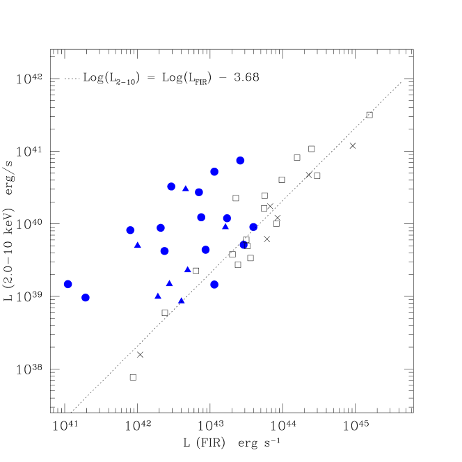
   Figure 3: 2.0–10 keV vs. FIR luminosities of star-forming galaxies and LLAGN. Filled triangles: LINERs, filled circles: Seyfert galaxies. Open symbols as in Fig. (1); line: Eq. (9).

Following this investigation, we have analyzed the relations between radio/FIR/X-ray luminosities for the spiral galaxies in the Terashima et al. (2002) sample of LLAGN, drawn from HFS97 and observed with ASCA, comprising 7 LINERs and 15 Seyfert’s with $4\cdot 10^{39}\lesssim L_{2-10}\lesssim 5\cdot 10^{41}$ erg s^-1. We find that the X-ray/FIR and X-ray/radio luminosity ratios generally exceed those of star-forming galaxies, but about one third of the objects have ratios falling on the same locus of the star-forming galaxies (Fig. 3). Therefore, the nuclear X-ray emission of these last LLAGN must be comparable to or weaker than the emission from star formation related processes. Moreover, the infrared (IRAS band) colours of these objects are also similar to those of star-forming galaxies, and completely different from those of QSOs, thus suggesting that the FIR luminosities of LLAGN may be powered by star formation.

4 Comparison with other X-ray based SFR indicators

Our inference of using the 2–10 keV luminosity as a SFR indicator is consistent with a study on Lyman-break galaxies by Nandra et al. (2002) who have extrapolated the David et al. (1992) FIR/soft X-ray relation to the hard X-ray band obtaining a SFR/2–10 keV luminosity relation within $10\%$ of our Eq. (12). From a stacking analysis of Chandra data for a sample of optically selected Lyman-break and Balmer-break galaxies in the HDFN they find a good agreement of the average SFR as estimated from X-ray and extinction-corrected UV luminosities.

A similar derivation of an $L_{\rm X}$-SFR relation has been performed by Bauer et al. (2002), using 0.5–8.0 keV and 1.4 GHz luminosities of a joint sample of 102 nearby late-type galaxies observed with Einstein (Shapley et al. 2001) and of 20 galaxies with emission line spectra in the Chandra Deep Field North.

Grimm et al. (2003); (see also Gilfanov et al. 2004b) have recently shown that the luminosity function of High Mass X-ray Binaries (HMXB) can be derived from a universal luminosity function whose normalization is proportional to the SFR. They also show that, due to small numbers statistics, a regime exists, in which the total X-ray luminosity grows non-linearly with the number of point sources. This has the consequence that also the total X-ray luminosity vs. SFR relationship is non-linear in the same regime, namely for SFR below $4-5M_{\odot}$/yr. Although this might seem at odds with our findings of Sect. 2, it is not really so, since Grimm et al. (2003) analysis only refers to the contribution from HMXB. It has been shown (Gilfanov et al. 2004a) that once the Low Mass X-ray Binaries are taken into account, their result are in agreement with the X-ray/radio/FIR correlations we found. However, the number of LMXB should be related with the integrated star formation over a much longer time than the HMXB (e.g. several Gyr) and thus not trace the current SFR. Mantaining both the radio/FIR/X-ray correlations, and the interpretation of the emission in these bands as powered by recent star formation, should require that also the FIR and radio emission are non-linearly related with the SFR; this has indeed been suggested for the radio (Bell 2003). As to the FIR emission, further investigations will be required to clarify its relation with the warm and dust component; thus at present the question stays open.

Author	SFR estimate	Method
Ranalli et al. (2003)	SFR$=2.0\cdot 10^{-40}L_{2-10}$	radio/FIR/X-ray correlations,
	SFR$=2.2\cdot 10^{-40}L_{0.5-2}$	23 galaxies obs. w. ASCA
Nandra et al. (2002)	SFR$=1.8\cdot 10^{-40}L_{2-10}$	0.5–4.5 keV/FIR correlation
		in David et al. (1992)
Bauer et al. (2002)	SFR$=(1.7\pm 0.5)\cdot 10^{-43}\cdot$	102 galaxies with Einstein
	$\cdot L_{0.5-8}^{1.07\pm 0.08}$	+20 galaxies in the CDFN
Grimm et al. (2003)	SFR$=1.5\cdot 10^{-40}L_{2-10}$	theory + 23 nearby
	($M>4.5M_{\odot}$/yr)	galaxies (mainly Chandra
	SFR$=(3.8\cdot 10^{-40}L_{2-10})^{0.6}$	data)
	($M<4.5M_{\odot}$/yr)

   Table 2: A comparison of different SFR indicators based on the X-ray luminosity.

5 NGC 3256: a case for intrinsic absorption

We present the test case of NGC 3256, a luminous dusty merger remnant included in the supplementary sample. Detailed studies at several wavelengths (radio: Norris & Forbes 1995, IR: Kotilainen et al. 1996, optical: Lípari et al. 2000, X-ray: Moran et al. 1999, Lira et al. 1999) have shown that the energetic output of this galaxy is powered by star formation occurring at several locations, but mainly in the two radio cores discovered by Norris & Forbes (1995) and also detected with Chandra (LABEL:fig_3256).

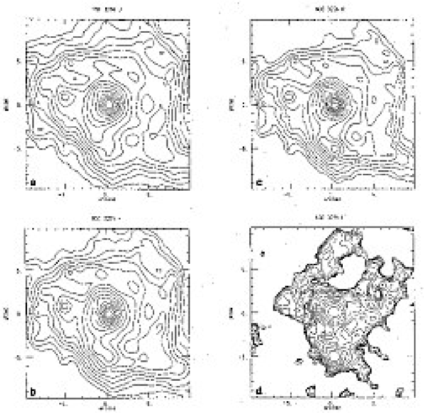
   Figure 4: A sequence of infrared images of the centre of NGC3256 at increasing wavelenghts, from Kotilainen et al. (1996). The southern nucleus lies behind a dust lane, and becomes visible in the L^′ band. The two nuclei are the brightest sources in NGC3256 in the radio and 2.0–10 keV bands (cfr. LABEL:fig_3256).

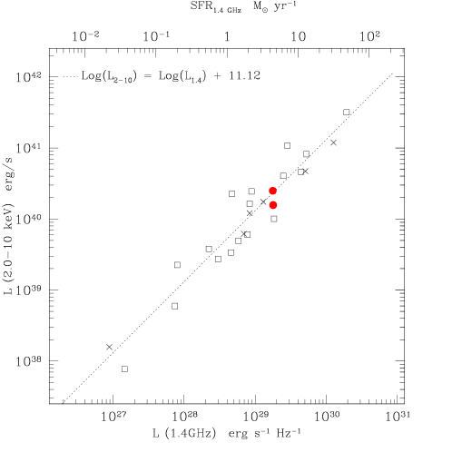
   Figure 5: 2.0–10 keV vs. radio luminosities of the two nuclei of NGC 3256 (filled circles). The upper and lower circles represent the north and south nucleus, respectively. The other symbols (same as in Fig. 1) represent the other galaxies in the sample.

The 3 and 6 cm radio maps (Norris & Forbes 1995) reveal two distinct, resolved (FWHM $\sim 1.2\hbox{${}^{\prime\prime}$}$) nuclei and some fainter diffuse radio emission. Separated by $5\hbox{${}^{\prime\prime}$}$ in declination, the two cores dominate the radio emission, the northern one being slightly (15%) brighter. They share the same spectral index ($\alpha\sim 0.8$). Chandra observations (LABEL:fig_3256) have shown that they also have similar 2–10 keV fluxes. Both of them follow the radio/hard X-ray correlation (Fig. 5), while only the northern one follows the radio/soft X-ray correlation. At other wavelengths the northern core is the brightest source in NGC 3256, while the southern one lies behind a dust lane and is only detected in the far infrared ($\lambda>10\mu$m), as clearly shown in the sequence of infrared images at increasing wavelengths in Kotilainen et al. (1996).

Although the southern core appears as a bright source in the hard X-rays ($E>2$ keV), there are not enough counts to allow an accurate spectral fitting. However, it is still possible to constrain the absorbing column density by assuming a template spectrum, such as a simple power-law or the spectrum of the northern core, leading (after standard processing of the Chandra archival observation of NGC 3256) to an intrinsic $N_{\rm H}=(2.2\pm 1.0)\cdot 10^{22}$ cm^-2 ($N_{\rm H,Gal}=9.5\cdot 10^{20}$ cm^-2), fully consistent with the $A_{\rm V}=10.7$ estimated by Kotilainen et al. (1996) from infrared observations. We note that 84% of the 2–10 keV flux and only 10% of the 0.5–2 keV one are transmitted through this column density. Thus, while the flux loss in the hard band is still within the correlation scatter, the larger loss in the soft band throws the southern nucleus off the correlation of Eq. (6).

6 Effect of variability on the flux estimate

IC 342: variability of ULXs

In the ASCA observations, the X-ray emission of IC 342 (a face-on spiral galaxy at 3.9 Mpc) is powered by three main sources; two of them (source 1 and 2 according to Fabbiano & Trinchieri 1987) are ultraluminous X-ray binaries (ULX) while source 3 is associated with the galactic centre. Observations with higher angular resolution (ROSAT HRI, Bregman et al. 1993) showed that sources 1 and 2 are point-like while source 3 is resolved in at least three sources. Our main concern in determining the flux of this galaxy is the variability of the two ULX, which was assessed by a series of observations spanning several years: IC342 was first observed by Einstein in 1980 (Fabbiano & Trinchieri 1987), then by ROSAT in 1991 (Bregman et al. 1993), by ASCA in 1993 (Okada et al. 1998) and 2000 (Kubota et al. 2001), and by XMM-Newton in 2001.

In Table 3 we report soft X-ray fluxes for sources 1 and 2. We have chosen the soft X-ray band due to the limited energy band of both Einstein and ROSAT; the fluxes observed with these satellites were obtained from the count rates reported in Fabbiano & Trinchieri (1987) and Bregman et al. (1993) assuming the powerlaw and multicolor disk examined in Kubota et al. (2001) for source 1 and 2 respectively; we take ASCA 1993 and 2000 fluxes from Kubota et al. (2001). XMM-Newton archival observations were reduced by us with SAS 5.3 and the latest calibrations available.

Source 1 was in a low state ($F_{0.5-2}\sim 3-5\cdot 10^{-13}$ erg s^-1) during the 1980, 1991, 2000 and 2001 observations, and in a high state ($F_{0.5-2}\sim 16\cdot 10^{-13}$ erg s^-1) during the 1993 observation. The broad-band (0.5-10 keV) spectrum changed, its best-fit model being a disk black-body in 1993 and a power-law in 2000 and 2001. Source 2 has also shown variability, its 0.5-2.0 keV flux oscillating between $0.52\cdot 10^{-13}$ (ASCA 2000) and $2.56\cdot 10^{-13}$ (ASCA 1993) erg s^-1; the main reason for this variability being the variations in the strongly absorbing column density, which was $9.9\cdot 10^{21}$ cm^-2 in 1993 and $18\cdot 10^{21}$ cm^-2 in 2000. The spectrum was always a power-law.

The high state for source 1 seems thus to be of short duration, and we feel confident that its time-averaged flux may be approximated with its low state flux. We thus choose to derive our flux estimate for IC 342 from the ASCA 2000 observation, estimating the variation for the total flux of the galaxy caused by source 2 variability to be less than 10%.

		Src 1 Flux		Src 2 Flux
Year	Mission	bb	po	po
1980	Einstein	2.7	4.1	0.85
1991	ROSAT	3.3	2.7	1.3
1993	ASCA	16		2.6
2000	ASCA		5.0	0.52
2001	XMM-Newton		4.1	1.3

   Table 3: 0.5–2.0 keV fluxes (in $10^{-13}$ erg s^-1 cm^-2) for sources 1 and 2 in IC 342 for a blackbody (bb) and a power-law (po) model.

Variability in M82

Hard (2–10 keV) X-ray variability in M82 was reported in two monitoring campaigns with ASCA (in 1996, Ptak & Griffiths 1999) and RXTE (in 1997, Rephaeli & Gruber 2002). M82 was found in “high state” (i.e. $4\cdot 10^{-11}\lesssim f_{2-10}\lesssim 7\cdot 10^{-11}$) in three out of nine observations with ASCA and in 4 out of 31 observations with RXTE. In all the other observations it was in a “low state” ($2\cdot 10^{-11}\lesssim f_{2-10}\lesssim 3.5\cdot 10^{-11}$). A low flux level was also measured during the observations with other experiments: HEAO 1 in 1978 (Griffiths et al. 1979); Einstein MPC in 1979 (Watson et al. 1984); EXOSAT in 1983 and 1984; BBXRT in 1990; ASCA in 1993 (Tsuru et al. 1997); BeppoSAX in 1997 (Cappi et al. 1999); Chandra in 1999 and 2000, XMM-Newton in 2001. No variability was instead detected in the 0.5–2.0 keV band (Ptak & Griffiths 1999).

The high state has been of short duration: less than 50 days in 1996, when it was observed by ASCA, and less than four months in 1997. A monitoring campaign was also undertaken with Chandra, which observed M82 four times between September 1999 and May 2000. We reduced the archival data, and found that the galaxy was always in a low state, with its flux slowly increasing from $1.2\cdot 10^{-11}$ to $2.9\cdot 10^{-11}$.

We do not attempt a detailed analysis of the variability (see Rephaeli & Gruber 2002); however, we feel confident that, given the short duration of the high states and the fact that the difference between high- and low state flux is about a factor 2, the time-averaged flux of M82 can be approximated with its low state flux. We thus choose to derive our flux estimate for M82 from the BeppoSAX 1997 observation ($f_{2-10}=2.9\cdot 10^{-11}$ erg s^-1 cm^-2), estimating the uncertainty caused by variability to be around $30\%$.

Chapter 2 Star-forming galaxies in the Hubble Deep Field

The X-ray and radio observations in deep fields reach limiting fluxes deep enough to detect star-forming galaxies at large redshifts $z\gtrsim 1$. Thus they can be used to check whether the radio/X-ray relation holds also for distant galaxies.

We consider the surveys performed in the Hubble Deep Field North (HDFN), a region of sky at a high Galactic latitude which was selected because of the very low extinction due to our Galaxy, centred at the (J2000) coordinates $12^{\rm h}\ 36^{\rm m}\ 49.5^{\rm s}\ +62^{\circ}\ 12^{\prime}\ 58\hbox{${}^{\prime\prime}$}$. The Chandra survey centred on the HDFN region (also called Chandra Deep Field North, CDFN) was initially performed for an assigned time of 1 million seconds (Brandt et al. 2001) and then extended with one other million secondes (Alexander et al. 2003). It is customary to refer to the intermediate data release as the ‘1 Ms survey’ and to the final one as the ‘2 Ms survey’. The final survey reaches a limiting flux of $2.5\cdot 10^{-17}$ erg s^-1 cm^-2 in the 0.5–2.0 keV band for sources in the centre of the field. The HDFN was also imaged at radio wavelengths, with the Very Large Array (VLA) at 8.4 GHz (Richards et al. 1998) and at 1.4 GHz (Richards 2000), and with the Westerbork Synthesis Radio Telescope (WSRT) at 1.4 GHz (Garrett 2000). The limiting fluxes for these radio surveys are all around 0.05 mJy.

We searched for X-ray counterparts of radio sources in the Richards et al. (1998) catalogue which contains optical and IR identifications allowing the selection of candidate star-forming galaxies. Our selection criterium has been to include all galaxies with Spiral or Irregular morphologies, known redshifts and no AGN signatures in their spectra (from Richards et al. 1998 or Cohen et al. 2000). The X-ray counterparts were initially searched for in the 1 Ms catalogue (Brandt et al. 2001). When the final data release was made available, we reduced the X-ray data, generated a catalogue, and we looked for X-ray counterpars of the radio sources. Our data reduction method followed rather closely the one described in Brandt et al. (2001). Unless otherwise stated, all data reported here come from reduction of the complete 2 Ms CDFN survey.

The mean positional uncertainties of both Chandra (for on-axis sources) and the VLA are $\sim 0.3\hbox{${}^{\prime\prime}$}$, which added in quadrature give $\sim 0.5\hbox{${}^{\prime\prime}$}$. Using this value as the encircling radius for coordinate matching 5 galaxies were found in Brandt et al. (2001). However, there are two effects that may increase this value:

1. the shape and width of the Chandra PSF strongly depend on the off-axis and azimutal angles. Since the 2 Ms HDFN data consist of 20 observations with different pointing directions and position angles, there is no unique PSF model even for near on-axis sources;

2. a displacement between the brightest radio and X-ray positions, induced e.g. by an ultraluminous X-ray binary placed in a spiral arm and dominating the X-ray emission.

Thus, by making cross-correlations with increasing encircling radii we found that the number of coincidences increases up to a radius of $1.0\hbox{${}^{\prime\prime}$}$, yielding 7 matchings. There are no further coincidences up to a radius of several arcsecs, indicating that the sample should not be contamined by chance coincidences.

By performing the same cross-correlation on the 2 Ms CDFN data, we added 4 more galaxies with coincidences within $1.0\hbox{${}^{\prime\prime}$}$, thus totalling 11 sources. One of these the 11 galaxies was dropped since it is probably an AGN on the basis of X-ray spectral and variability properties, as discussed below. The selected objects are listed in Table 1. Fluxes at 1.4 GHz and spectral slopes were retrieved from Richards (2000) in 9 cases, and from Garrett (2000) in one case.

Chandra	VLA
CXOHDFN J123634.4+621212 (134)	3634+1212
CXOHDFN J123634.5+621241 (136)	3634+1240
CXOHDFN J123637.0+621134 (148)	3637+1135
CXOHDFN J123651.1+621030 (188)	3651+1030
CXOHDFN J123708.3+621055 (246)	3708+1056
CXOHDFN J123716.3+621512 (278)	3716+1512
not present in Brandt et al. (2001)	3644+1249
id.	3701+1146
id.	3638+1116
id.	3652+1354

   Table 1: Identification of candidate star-forming galaxies in the Richards et al. (1998) catalogues with their X-ray counterpart (Brandt et al. 2001). Where applicable, the entry number in the Chandra catalogue is shown in parenthesis.

   Figure 1: Observer’s-frame hardness ratios for the 7 galaxies in the CDFN catalogue by Brandt et al. (2001); there are only upper limits since none is detected in the 2–8 keV band. The dotted lines show the loci for power-law spectra with slope $\Gamma=2.1$ and different intrinsic rest-frame absorption; the dashed lines are for spectra of different slopes and no intrinsic absorption.

While the rest-frame 0.5–2.0 and 2.0–10 keV luminosities could be obtained by K-correcting the observer’s frame counts, this would imply the assumption of a spectral shape; but none of the deep field galaxies is individually detected in the hard band, so that any constraint on their spectra obtained with the use of a hardness ratio diagram is too loose to be significant (Fig. 1). However this problem may be partially circumvented by resizing the X-ray bands in the observer’s frame according to the redshift of the objects – i.e. the counts extracted with this method correspond to the photons actually emitted in the rest-frame 0.5–2.0 and 2–8 keV bands. It is therefore possible to give better constraints to the spectra of the deep field galaxies and derive better estimates of their luminosities.

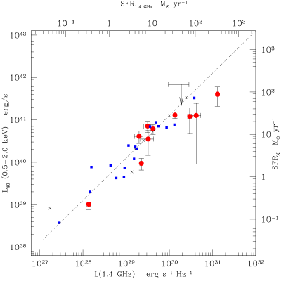
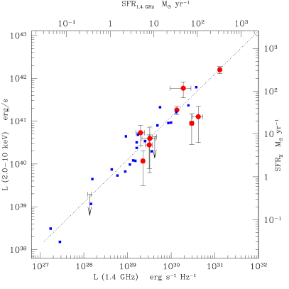
   Figure 2: The radio/X-ray luminosity relation for galaxies in the Hubble Deep Field (filled circles). Squares: local galaxies as in Fig. (1); dotted lines: linear fits for local galaxies (Eq. 6). Besides the 10 deep field galaxies discussed in the text, here is shown also the point relative to the galaxy hd2-264.1 (in the Hubble Deep Field, at $z=0.475$) which is the only galaxy from the sample of Cardiel et al. (2003) to have an X-ray detection ($L_{0.5-2}=1.5\cdot 10^{41}$ erg/s, $L_{2-10}=5\cdot 10^{40}$ erg/s, $L_{1.4}=6\cdot 10^{29}$ erg/s/Hz).

Thus, we have redefined the soft and hard bands as the [0.5; $2.0/(1+z)$] and [$2.0/(1+z)$; $8/(1+z)$] intervals, respectively. Another advantage of this procedure is that the higher the redshift, the more akin the new hard band is to the zone of maximum sensitivity of Chandra ($\sim 1-4$ keV). Note that since the ACIS-I detector has almost no sensitivity below 0.5 keV, we fixed this energy as the lower limit for count extraction. For the two highest redshift galaxies, this reduces the soft band to 0.5–0.9 keV, still significantly larger than the ACIS-I energy resolution (FWHM $\lesssim 100$ eV).

We extracted counts in circular regions (with radii of 5 pixel, i.e. $\sim 2.5\hbox{${}^{\prime\prime}$}$) around our selected targets; the background counts were taken in circular annuli surrounding the targets, with outer radii of 12 pixels ($\sim 6\hbox{${}^{\prime\prime}$}$), respectively. Counts and rates are reported in Table 2. Best-fit slopes reproducing the soft/hard count ratio were derived by assuming a power-law spectrum with Galactic absorption. We find that all objects have spectral slopes falling in the range $\Gamma\sim 1.5$–$2.7$ (Table 2). To check whether these spectra are consistent with those of the galaxies in the local sample we calculated the observed soft/hard flux ratio for galaxies in the local sample of Sect. 1: the median value for this flux ratio is 0.95 leading to a slope $\Gamma\sim 2.1$. The count ratios for each of the six deep field galaxies are consistent within 1–2$\sigma$ with the $\Gamma\sim 2.1$ slope.

One of the sources (#194 in Brandt et al. 2001, not shown in Table 2, with $z=1.275$) has an upper limit on the soft X-ray counts and a count ratio not consistent at the $5\sigma$ level with the unabsorbed $\Gamma\sim 2.1$ spectrum: it requires an inverted spectrum ($\Gamma<0.1$) if no absorption is assumed, otherwise, if we assume $\Gamma=2.1$, the intrinsic absorbing column has to be $N_{\rm H}\gtrsim 3.4\cdot 10^{22}$ cm^-2. We also find that the flux of this source is strongly variable, since all detected counts were recorded in the first half of the survey, and no one in the second half which was performed about one year later. Thus, from its spectral and variability properties, we classified this source as an AGN and dropped it from the sample considered here.

With the best-fit slopes we derived soft and hard band fluxes and luminosities (Fig. 2). The linear radio/X-ray correlations hold also for the Deep Field galaxies; the dispersion of the relations given in Sect.2 is not changed by the inclusion of the deep field objects.

A similar result was also found by Bauer et al. (2002) by analyzing a sample of 20 galaxies selected at 1.4 GHz in the Chandra Deep Field North. Their sample is partly overlapping with the one here described (not identical, since ours was selected at 8.4 GHz).

Fluxes and Luminosities: Deep Sample
			Soft X-rays			Hard X-rays				Radio
Source		$z$	Net Cts.	$F$	$L$	Net Cts.	$F$	$L$	$\Gamma$	$F$	$L$	$\alpha$
134	3634+1212	0.456	55	20	13	39	28	18	1.9	210	1.4	0.7
136	3634+1240	1.219	11	5.6	40	44	22	160	1.4	180	13	0.7
148	3637+1135	0.078	27	7.2	0.10	—	$<$4.6	$<$0.065	—	96	0.014	0.6
188	3651+1030	0.410	24	12	6.1	4.3	$<$2.8	$<$1.4	—	83	0.42	0.6
246	3708+1056	0.423	22	7.5	4.1	13	9.8	5.3	1.4	36	0.20	0.4
278	3716+1512	0.232	22	6.6	0.94	8.7	8.2	1.2	1.4	160	0.23	0.2
new	3644+1249	0.557	9.2	3.4	3.5	7.3	3.8	3.9	2.1	31	0.32	0.7
new	3701+1146	0.884	6.7	3.8	12	6.9	2.8	8.9	3.4	93	3.0	0.5
new	3638+1116	1.018	4.6	2.8	13	7.4	2.8	13	2.2	92	4.2	1.1
new	3652+1354	1.355	3.8	$<$2.4	$<$23	16	6.2	59	—	20	1.9	—

   Table 2: Data for deep field galaxies (counts, fluxes, luminosities). $\Gamma$ is the best fit X-ray slope (photon index), $\alpha$ the radio slope (energy index). Sources are identified via their entry number in the Brandt et al. (2001) catalogue (cfr. Table 1) and their denomination in the VLA catalogue (Richards et al. 1998). X-ray fluxes in $10^{-17}$ erg s^-1 cm^-2, radio fluxes in $\mu$Jy. X-ray luminosities in $10^{40}$ erg s^-1, radio luminosities in $10^{30}$ erg s^-1 Hz^-1. X-ray counts are extracted in redshifted bands (soft band $:=0.5$–$2.0/(1+z)$ keV, hard band $:=2.0/(1+z)$–$8/(1+z)$ keV); the counts shown here are already background subtracted. X-ray fluxes and luminosities are in rest-frame 0.5–2.0 and 2.0–10 keV bands, radio ones at rest-frame 1.4 GHz. For source #194, the absorbed flux and luminosity are quoted. The unabsorbed luminosity is $\lesssim 4\cdot 10^{42}$ erg s^-1. Upper limits on fluxes and luminosities were assigned whenever the estimated error on the flux was of the same magnitude of the flux.

Chapter 3 The X-ray number counts and luminosity function of galaxies

An estimate of the contribution of star-forming galaxies to the cosmic X-ray background (XRB) has been attempted several times (e.g. Bookbinder et al. 1980, Griffiths & Padovani 1990, Moran et al. 1999). The main purpose for the earlier studies was the possibility to explain the flatness of the XRB spectrum via the X-ray binaries powering the X-ray emission of these galaxies (High Mass X-ray Binaries have flat spectra with slopes $\Gamma\sim 1.2$). Although AGN have since a long time been recognized to provide by far the most important contribution to the XRB (Setti & Woltjer 1989; Comastri et al. 1995), the ongoing deep Chandra and XMM-Newton surveys offer unique opportunities to both test the AGN models and pin down the contribution from other kind of sources.

A study of the X-ray number counts and of the luminosity function (LF) of galaxies is also valuable in the perspective of studying the evolution of the X-ray luminosity function (XLF) and the cosmic star formation history. In this chapter, the X-ray luminosity function and number counts of star forming galaxies are determined making use of different approaches, such as objects selection from X-ray surveys, conversion of radio and FIR LFs and number counts. An estimate is also performed of the contribution to the XRB. Finally, the possibilities to use X-ray observations to determine the cosmic star formation history are discussed.

1 The X-ray luminosity function of galaxies

The availability of multiwavelength photometry and spectral information (Barger et al. 2003; Szokoly et al. 2004) for the X-ray objects in the Chandra Deep Fields allows a direct identification of the star forming galaxies in these surveys. This is however a difficult task, for two reasons: i) at the limiting fluxes of current X-ray surveys, the majority of detected sources are AGN; ii) it may prove to be difficult, for objects at redshifts $z\sim 1$, to distinguish a bright starburst galaxy from a low luminosity type-2 Seyfert galaxy (cfr. Sect. 5). Thus, in order to pick up normal galaxies in the X-ray survey samples, extreme care has to be put in the choice of the selection tools. We will not venture into a comprehensive discussion of the selection tools (good starting points for this might be Machalski & Condon 1999 and Norman et al. 2004), but just briefly illustrate a few of them that will be used throughout this chapter.

A direct determination of the X-ray luminosity function (XLF) of galaxies has been recently attempted in Norman et al. (2004), where a sample was defined containing 210 galaxies with known redshift from the Chandra Deep Field catalogues (Alexander et al. 2003; Giacconi et al. 2002). A Bayesian approach was chosen to derive a selection probability from the values of three different parameters:

• the 0.5–2.0 keV X-ray luminosity for star forming galaxies is usually less than $\sim 10^{42}$ erg/s;

• star forming galaxies have a softer spectrum than AGN; this translates in selecting objects with an hardness ratio $HR\lesssim-0.8$ (with $HR=(H-S)/(H+S)$, where $H$ and $S$ represent the 2.0–10 and 0.5–2.0 keV fluxes respectively);

• an X-ray/optical flux ratio $\mbox{Log}(F_{{\rm X-ray}}/F_{{\rm opt}})<-1$ (see below).

The optical flux is defined as

$$\mbox{Log}\ F_{\rm opt}=-0.4R-5.5$$ (1)

were $R$ is the red magnitude in the Kron-Cousins system. An X-ray/optical flux ratio equal (in logarithm) to $-1$ is usually taken as an approximate boundary between normal galaxies and Seyferts (Maccacaro et al. 1988; see also McHardy et al. 2003).

We will consider the local differential luminosity function $\varphi(L){\rm d}\mbox{Log}L$, which is the comoving number density of sources per logarithmic interval of luminosity. A binned luminosity function (LF) was derived with the method developed in Page & Carrera (2000), which is a variant on the classical $1/V_{\rm max}$ method by Schmidt (1968). In a given bin of redshift and luminosity, the density of galaxies may be written as

$$\varphi\sim\frac{N}{\int_{L_{\rm min}}^{L_{\rm max}}\int_{z_{\rm min}}^{z_{{\rm max}(L)}}\int_{0}^{4\pi}\frac{{\rm d}V}{{\rm d}z\,{\rm d}\Omega}\,{\rm d}\Omega\,{\rm d}z\,{\rm d}L}$$ (2)

where ${\rm d}V/{\rm d}z{\rm d}\Omega$ is the comoving volume per unit steradian sampled by the surveys. For a flat universe with non-zero cosmological constant we may take

$$\frac{{\rm d}V}{{\rm d}z}=4\pi\left(\frac{c}{H_{0}}\right)^{3}\frac{1}{E(z)}\left[\int_{0}^{z}\frac{{\rm d}z^{\prime}}{E(z^{\prime})}\right]^{2}$$ (3)

with

$$E(z)=\sqrt{\Omega_{\rm M}(1+z)^{3}+\Omega_{\Lambda}}.$$ (4)

The redshift distribution of the Norman et al. (2004) sample is shown in Fig. (2). Two redshift bins were considered, $z\leq 0.5$ and $0.5<z\leq 1.2$, with mean redshifts $z=0.27$ and 0.79 respectively, in order to have a comparable number of galaxies in both bins.

   Figure 1: Redshift distribution for the Bayesian sample of X-ray selected normal galaxies defined in Norman et al. (2004). Dotted and dashed line: redshift distributions for galaxies in the Chandra Deep Fields South and North, respectively. Continous line: sum of the North and South subsamples.

   Figure 2: X-ray luminosity function for the galaxies in the Bayesian sample by Norman et al. (2004). Triangles: LF of objects with $z\leq 0.5$; circles: LF of objcts with $z>0.5$. The median redshift of the two bins are $z=0.27$ and 0.79 respectively, thus the two data sets may be regarded as the XLFs at the median redshifts; the evolution of the LF from $z=0.27$ to $z=0.79$ is clearly visible.

The XLF is shown in Fig. (2). Norman et al. (2004) also determined the evolution of the LF, by fitting the XLFs in the two redshift bins with two power laws. Considering a pure luminosity evolution, they found $L(z)/L(0)=(1+z)^{2.7}$. This result will be checked in the following sections against FIR- and radio-based determinations of the XLF.

2 Determining the XLF from the FIR and radio luminosity functions

Infrared surveys are a powerful method to select star forming, spiral galaxies, since the bulk of the far and near infrared emission is due to reprocessed light from star formation, with AGN representing only a minor population (de Jong et al. 1984; Franceschini et al. 2001; Elbaz et al. 2002). In the following, we summarize the current determinations of the FIR luminosity functions, which are then converted to the X-rays.

We will only consider a pure density evolution of the form $(1+z)^{\eta}$, which is the simplest and most used form by the authors of the papers from which we draw the FIR LFs. This is equivalent, in a more rigorous formalism, to a bivariate LF of the form $\varphi_{\rm b}(L,z)\,{\rm d}\mbox{Log}L\,{\rm d}z$ with the assumption that the LF is separable for $L$ and $z$, so that we may write $\varphi_{\rm b}(L,z)=\varphi(L)(1+z)^{\eta}$.

   Figure 3: Left panel: Redshift distribution for galaxies in the IRAS PSC$z$ survey, from Saunders et al. (2000). Right panel: Luminosity-redshift relation for galaxies in the ELAIS survey, from Serjeant et al. (2004).

Saunders et al. (1990) defined a sample of 2,818 galaxies matching common selection criteria from different IRAS samples, with a flux limit around 0.6 mJy at 60$\mu$, completeness at 98% level, redshifts $z\lesssim 0.05$, and derived a $60\mu$ luminosity function. The best-fit model has the shape

$$\varphi(L)=\varphi^{*}\left(\frac{L}{L^{*}}\right)^{1-\alpha}\exp\left[-\frac{1}{2\sigma^{2}}\mbox{Log}^{2}_{10}\left(1+\frac{L}{L^{*}}\right)\right]\quad\rm{Mpc}^{-3}$$ (5)

with parameters at present epoch

$$\varphi^{*}=(2.6\pm 0.8)\cdot 10^{-2}\,h^{3}\,{\rm Mpc}^{-3},\alpha=1.09\pm 0.12,$$

$$\sigma=0.72\pm 0.03\mbox{ and }L^{*}=(2.95_{-1.21}^{+3.06})\cdot 10^{8}\,h^{-2}\,L_{\odot}$$ (6)

(shown as the dotted curve in Fig. 5) and the evolution (parameterized as pure density evolution)

$$(1+z)^{6.7\pm 2.3}.$$ (7)

   Figure 4: IRAS and ISO local (i.e. $z=0$) luminosity functions. Solid curve: IRAS 60$\mu$ LF from Takeuchi et al. (2003). Dotted curve: IRAS 60$\mu$ LF from Saunders et al. (1990). The two IRAS LFs coincide at bright luminosities. Dashed curve: ISO 90$\mu$ LF from Serjeant et al. (2004); the shaded area corresponds to the 1$\sigma$ errorbar. While the IRAS LFs are well constrained in the whole range of luminosities shown here, the ISO LF suffers from incompleteness for $L\lesssim 10^{9}L_{\odot}$. The monocromatic luminosities have been converted to bolometric ones by assuming $\nu L_{\nu}={\rm cost}$. $H_{0}=70$ is assumed.

   Figure 5: IRAS, ISO, and radio luminosity functions converted to the X-rays. Solid curve: IRAS 60$\mu$ LF from Takeuchi et al. (2003). Dotted curve: IRAS 60$\mu$ LF from Saunders et al. (1990). Points: ISO 90$\mu$ LF from Serjeant et al. (2004). Dashed curve: radio LF from Machalski & Godlowski (2000).

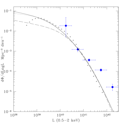
   Figure 6: Comparison of the X-ray luminosity function with the FIR- and radio-derived ones. Symbols as in Figs. (2, 5). The FIR- and radio-based LFs have been evolved (see text) to the median redshifts of the two bins in which the XLF was calculated (i.e. $z=0.27$ in the left panel, $z=0.79$ in the right panel). For the Saunders et al. (1990) IRAS LF, the milder evolution determined by Takeuchi et al. (2003) was used.

The $60\mu$ luminosity function was revised by Takeuchi et al. (2003) by enlarging the galaxy sample. 15,411 galaxies from the Point Source Catalog Redshift (PSC$z$) were used, covering 84% of the sky with a flux limit of 0.6 mJy at $60\mu$. Using the same parameterization of Eq. (5), Takeuchi et al. (2003) found

$$\varphi^{*}=(2.60\pm 0.30)\cdot 10^{-2}\,h^{3}\,{\rm Mpc}^{-3},\alpha=1.23\pm 0.04,$$

$$\sigma=0.724\pm 0.01\mbox{ and }L^{*}=(4.4\pm 0.9)\cdot 10^{8}\,h^{-2}\,L_{\odot}.$$ (8)

In Fig. 5 it is shown as the dotted curve. They also found that the $(1+z)^{6.7}$ density evolution proposed by Saunders et al. (1990) is not consistent with their sample. A milder evolution $(1+z)^{3.4}$ is reported to be the best-fit description of the data. Note however that the redshift distribution of the PSC$z$ galaxies only span a very limited range (Fig. 3), thus the evolution exponent is very poorly constrained; this may also explain the factor-of-two difference in evolution between Takeuchi’s and Saunders’ results.

The LF at $90\mu$ was recently determined by the ELAIS survey team (Serjeant et al. 2001, 2004) with the PHOT and CAM instruments onboard the ISO satellite. It has not been fitted to a parametric form. Serjeant et al. (2004) also found that the evolution, if parameterized as a $(1+z)^{\eta}$ pure density form for $z\leq 1$ and no evolution beyond $z\sim 1$, has an exponent $2.4<\eta<4.6$ at 68% confidence; in the following we will assume $\eta=3$. The ELAIS LF is shown in Fig. 5 as the dashed curve, along with $1\sigma$ errors.

Conversion of the LF to the X-rays

The FIR luminosity functions may be converted to the X-rays using the approach first developed in Avni & Tananbaum (1986) (see also Georgantopoulos et al. 1999 and Norman et al. 2004).

$$\varphi_{\rm X}(\mbox{Log}\ L_{\rm X})=\int\limits_{0}^{+\infty}\varphi_{60\mu}(\mbox{Log}\ L_{60\mu})\,P\left(\mbox{Log}\ L_{\rm X}|\mbox{Log}\ L_{60\mu}\right){\rm d}\mbox{Log}\ L_{60\mu}$$ (9)

where $P\left(\mbox{Log}\ L_{\rm X}|\mbox{Log}\ L_{60\mu}\right)$ is the probability distribution for observing $L_{\rm X}$ for a given $L_{60\mu}$. Considering the radio/FIR relationship of Sect.2, this may be taken as a gaussian, yielding (for the 0.5-2 keV band)

$$P\left(\mbox{Log}\ L_{0.5-2}|\mbox{Log}\ L_{60\mu}\right)=\frac{1}{\sqrt{2\pi}\sigma}\,e^{-\frac{{\rm Log}\ L_{60\mu}+9.05-{\rm Log}\ L_{0.5-2}}{2\sigma^{2}}}$$ (10)

where $\sigma\sim 0.30$ as estimated in Sect. 2. To convert the ELAIS LF, a $S_{60\mu}/S_{90\mu}=0.66$ flux ratio may be derived by assuming $\nu L_{\nu}={\rm cost}$. The same figure can be obtained by considering a grey body law (Eq. 8) with $\beta=1$ and temperature $T=40$ K. The converted luminosity functions are shown in Fig. 5.

The XLF from the radio LF

Information from the radio surveys may also be used to derive an XLF. We consider the sample of radio detected galaxies in the Las Campanas Redshift Survey (Machalski & Condon 1999), which comprises 1157 galaxies with magnitude $R\leq 18.0$ and detected in the NRAO VLA Sky Survey (NVSS), i.e. brighter than 2.5 mJy beam^-1 at 1.4 GHz. These galaxies were classified as “starburst” (502 galaxies) or “AGN” (655 galaxies) on the basis of their FIR-radio flux ratios, 25$\mu$–60$\mu$ spectral indices and radio-optical flux ratios. Machalski & Godlowski (2000) derived the LFs for both classes of objects; here we consider only the “starbursts”.

For a LF with the functional form of Eq. (5), Machalski & Godlowski (2000) give the set of parameters

$$\varphi^{*}=(7.9_{-2.6}^{+3.8})\cdot 10^{-3}\,h^{3}\ {\rm Mpc}^{-3}{\rm dex}^{-1},\alpha=1.22\pm 0.27,$$

$$\sigma=0.61\pm 0.05\mbox{ and }\mbox{Log}\ L^{*}=(28.13\pm 0.37)\,h^{-2}\,{\rm\ erg\ s}^{-1}{\rm\ Hz}^{-1}.$$ (11)

We converted the radio LF into an XLF following the same method as in the previous paragraph, and considering the radio/X-ray relation of Sect. 2. The resulting XLF is shown in Fig. (5) along with the ones derived from the infrared surveys. The radio-based LF agrees well with the FIR-based ones for $L_{\rm X}\gtrsim 10^{40}$ erg/s, while it lies a factor of $\sim 2$ below the FIR-based LFs at lower luminosities.

The redshifts of the Las Campanas “starburst” galaxies are in the range $0.01\leq z\leq 0.075$. As in the case of the IRAS galaxies, this redshift range is too small to allow a reliable estimation of the evolution. The constraints on the evolution found by Machalski & Godlowski (2000) are too loose to either confirm of reject cosmic evolution for the Las Campanas galaxies.

3 Comparison with the XLF

To compare the pure luminosity evolution determined by Norman et al. (2004) with the pure density forms used above, we assume that the XLF may be well represented by a power law whose slope remains constant with varying redshifts. We remind, in fact, that for a power law shaped LF the two forms of evolution cannot be distinguished. In fact, it may easily be shown that a LF with pure luminosity evolution with the shape

$$\varphi_{0}L(z)^{-\alpha}=\varphi_{0}\left[L_{0}/(1+z)^{\eta}\right]^{-\alpha}$$ (12)

transforms into a pure density form as

$$\varphi(z)L_{0}^{-\alpha}=\varphi_{0}(1+z)^{\eta\alpha}L_{0}^{-\alpha}.$$ (13)

Since the XLF derived by Norman et al. (2004) has $\alpha\sim 1.1$, their $(1+z)^{2.7}$ luminosity evolution is equivalent to a $(1+z)^{2.9}$ density evolution — which agrees well with the evolution exponents found for the FIR LFs.

A comparison between the Norman et al. (2004) LF and the FIR/radio derived ones is made in Fig. (6). To make the comparison the easiest possible, the FIR/radio derived XLFs were evolved with their own evolution exponents, up to the mean redshifts of the two bins in which the Norman et al. (2004) was calculated. We found that the X-ray derived LF is in agreement with the FIR-radio derived LFs for $L_{\rm X}\lesssim 10^{41.5}$, but it is significantly flatter at its bright end ($L_{\rm X}\gtrsim 10^{41.5}$), where it has a density of galaxies which is one order of magnitude larger than that of the FIR-radio galaxies. This may be symptomatic of a residual fraction of low luminosity AGN in the sample used by Norman et al. (2004).

4 The observed X-ray Log $N$–Log $S$ of galaxies

We turn now to an analysis of the X-ray number counts of galaxies, since they represent the most direct testbed for both the selection criteria for normal galaxies in X-ray surveys, and for the shape and evolution of different LFs.

First we considered the Log $N$–Log $S$ of the sample defined in Norman et al. (2004) and discussed in Sect. 1, which is shown in Fig. (7) as the long-dashed histogram.

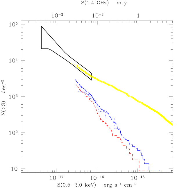
   Figure 7: X-ray counts in the Chandra Deep Fields. The thick, upper line and the horn-shaped symbol show the observed Log $N$–Log $S$ for all X-ray sources in the Deep Fields (Moretti et al. 2003) and the limits from the fluctuation analysis (Miyaji & Griffiths 2002a, b). The histograms show the Log $N$–Log $S$ for normal galaxies. Short-dashed (lower) histogram: sources with Log (X-ray/optical flux ratio) $<-1$. Dotted (middle) histogram: X-ray sources with a radio detection and an optical spectrum compatible with ion excition by H ii regions (Bauer et al. 2002). Long-dashed (upper) histogram: sources from the Bayesian sample of Norman et al. (2004).

Then we considered a sample defined in Bauer et al. (2002), who investigated the link between the faint X-ray and radio sources in the Chandra Deep Field North (CDFN); 11 sources from their catalogue could be reliably selected as star formation powered systems, on the basis of the reported optical spectrum (i.e. classified as “emission line galaxies”). By considering the sky coverage of the CDFN survey, as reported in Alexander et al. (2003), we derived the Log $N$–Log $S$ for these sources, which is shown in Fig. (7) as the dotted histogram.

We also considered 97 CDFN sources from Barger et al. (2003), which were selected for having an X-ray/optical flux ratio $\lesssim-1$. Although this selection criterium may be regarded as somewhat crude, it is indeed useful since it allows an immediate object selection with the least possible number of parameters. The resulting Log $N$–Log $S$ is plotted as the short-dashed histogram in Fig. (7).

We found that there is a quite good agreement (within a factor of 2–3) between the three observed Log $N$–Log $S$ described above. In the following sections, the X-ray Log $N$–Log $S$ will be checked against predictions made on the basis of the radio counts for the sub-mJy population and from the FIR and radio LFs.

5 X-ray number counts from radio surveys

We consider the radio sub-mJy population associated with faint blue galaxies at high redshifts ($22\lesssim V\lesssim 27$, $0.5\lesssim z\lesssim 1.5$; Windhorst et al. 1990) representing an early era of star formation in the universe (Haarsma et al. 2000). This strongly evolving population (Franceschini et al. 2001) accounts for the majority of the number counts below $\sim 0.5$ mJy (Windhorst et al. 1985) and contributes about half of the radio cosmic background at 1.4 GHz (Haarsma et al. 2000). The deepest radio surveys have been performed at 1.4 GHz (Richards 2000), 5 GHz (Fomalont et al. 1991) and 8.4 GHz (Richards et al. 1998). In order to derive the X-ray counts from the radio ones a full knowledge of the redshift distribution and spectra of the sources would be required. Under the simplifying assumption that the sub-mJy population lies at a redshift $\bar{z}$, so that the K-correction term is the same for all sources, the differential counts are obtained as

$$n(S_{\rm X})=n(S_{1.4}\cdot\kappa^{\rm X}_{1.4})$$ (14)

where $n(S)$ are the differential number counts, and $\kappa^{\rm X}_{1.4}=\kappa^{\rm X}_{1.4}(\bar{z},\alpha,\Gamma)$ is the X-ray band/1.4 GHz luminosity ratio (eqs.6,10) which depends on the redshift and on the radio and X-ray spectral indices via the K-correction:

$$\kappa^{\rm X}_{1.4}(\bar{z},\alpha,\Gamma)=\left.\kappa^{\rm X}_{1.4}\right|_{z=0}\cdot(1+\bar{z})^{-(\Gamma-1)+\alpha}$$ (15)

where, as customary, $\alpha$ denotes the radio spectral index (‘energy index’, defined by $S(\nu)\propto\nu^{-\alpha}$) and $\Gamma$ is the X-ray spectral index (‘photon index’, $S(\nu)\propto\nu^{1-\Gamma}$).

Concerning the sub-mJy Log $N$–Log $S$, Richards (2000) gives $n(S)=(2.51\pm 0.13)\cdot 10^{-3}S^{-2.38\pm 0.13}$ deg^-2 Jy^-1 as a best-fit to the differential number counts at 1.4 GHz in the range 45–1000$\mu$Jy, while Fomalont et al. (1991) find $n(S)=1.2\cdot 10^{-3}S^{-2.18\pm 0.19}$ at 5 GHZ in the range 16–1500 $\mu$Jy. The number density at 4 $\mu$Jy (as estimated from fluctuation analysis) is consistent with extrapolation of the 16–1500 $\mu$Jy slope.

The mean radio spectral index is in the range $\alpha=0.3$–0.7. Fomalont et al. (1991) report their distribution as having a moda of $\alpha=0.5$, a median of $\alpha=0.38$, and an average of $\alpha=0.28$ (indices measured between 1.5 and 5 GHz). From Richards (2000) data we find an average $\alpha=0.47$ (between 1.4 and 8.4 GHz), when we consider detections at both frequencies, and $\alpha=0.67$ when we consider only detections at 1.4 GHz and treat upper-limits at 8.4 GHz as detections. The latter, steeper slope is also more consistent with the average index of our HDFN sample (Table 2). Here we assume $\alpha=0.5$, and estimate the uncertainty in the K-correction due to the radio spectral index to be around a $15-20\%$.

According to the results of Sect.2, we further assume an average X-ray spectral slope $\Gamma=2.1$. For the sake of simplicity we also assume that the objects are placed at $\bar{z}\sim 1$, the mean redshift for the sub-mJy galaxies which, according to Windhorst et al. (1990), are distributed in the redshift interval 0.5–1.5 with a peak at $z\sim 1$. To estimate the effect on the counts due to the actual distribution of the sources in this redshift interval we consider a simplified case in which they are equally distributed at redshifts $z=0.5$, 1.0 and 1.5. Since the effect enters in the computations via the K-correction term, we find that the predicted number counts would increase by only $\sim 10\%$. As a last remark we notice that a fraction, as yet undefined, of the X-ray spectra might steepen at energies $\gtrsim 10$ keV, thus entailing a decrease in the predicted source counts; however, given the redshift range under consideration, the predicted soft X-ray source counts should not be affected.

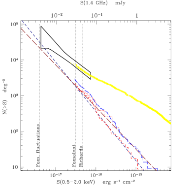
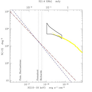
   Figure 8: X-ray counts derived from deep radio Log $N$–Log $S$ in the 0.5–2.0 (upper panel) and 2.0–10 keV (lower panel) bands. Histograms as in previous figures. The short-dashed lines represent the 1.4 GHz Log $N$–Log $S$ (Richards 2000) with K-corrections assuming $\bar{z}=1$, $\Gamma=2.1$ and $\alpha=0.5$. The long-dashed lines represent the Log $N$–Log $S$ by Fomalont et al. (1991) reported at 1.4 GHz with $\alpha=0.5$ (K-corrections like for the 1.4 GHz one). Thick line and horn-shaped symbols: total X-ray number counts and resuls from fluctuation analysis, respectively (see Fig. 7). The vertical dotted lines show the limiting sensitivities for the radio surveys. For easier reading, the horizontal scale is shown both in radio and X-ray fluxes, assuming the conversion factors of Sect. 2.

The X-ray number counts predicted with the above assumptions (i.e. $\alpha=0.5$, $\Gamma=2.1$) from Richards (2000) and Fomalont et al. (1991) Log $N$–Log $S$ are shown in Fig. (8), along with observed counts from Moretti et al. (2003) and limits from fluctuation analysis (Miyaji & Griffiths 2002a, b). The extrapolations of the radio Log $N$–Log $S$ below $\sim 50\mu$Jy and down to a few $\mu$Jy at 1.4 GHz ($\sim 6\cdot 10^{-18}$ erg s^-1 cm^-2 in the 0.5–2.0 keV band) are consistent with the limits from fluctuation analysis (Miyaji & Griffiths 2002b) and do not exceed the X-ray expected number counts. It should be noted, however, that eqs.(6,10) may not apply to the entire sub-mJy population. For instance, a fraction (up to a $15-20\%$, Haarsma et al. 2000) of the sources may still present a sizable contribution from an AGN. It follows that the derived Log $N$–Log $S$ should be regarded as an upper limit to the X-ray counts from star-forming galaxies.

As a final remark it should be pointed out that our results depend on the basic assumption of a strict linearity between the radio and X-ray luminosities. Had we assumed a non-linear relationship, such as Eq. (4) for the soft X-rays or Eq. (8) for the 2-10 keV band, we would have found an increase or decrease, respectively, of about $50\%$ in the predicted counts at a flux level around $10^{-17}$ erg s^-1 cm^-2.

6 X-ray counts from integration of the FIR and radio LFs

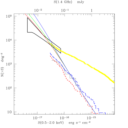
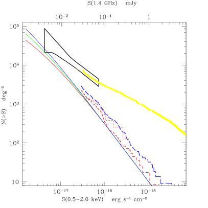
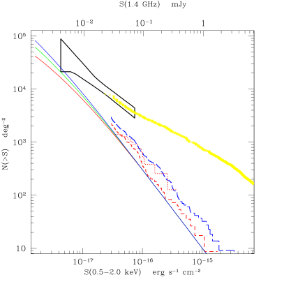
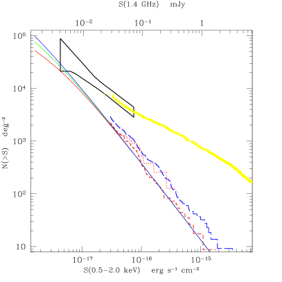
   Figure 9: X-ray counts derived from the IRAS luminosity function by Saunders et al. (1990). Left panel: $(1+z)^{6.7}$ density evolution; right panel: $(1+z)^{3.4}$ density evolution (see text). Thick line, horn shaped symbol and histograms as in the previous figures. The three thin curves, which converge at fluxes $\gtrsim 10^{-16}$ erg s^-1 cm^-2, show the number counts from the integral of the LF; lower curve: the LF was integrated with $z_{\rm max}=1.1$ and evolution as described in the text; upper curve: $z_{\rm max}=2$; middle curve: $z_{\rm max}=2$ but evolution stopped at $z=1$.

   Figure 10: X-ray counts derived from the IRAS luminosity function Takeuchi et al. (2003). Symbols as in Fig. (11).

   Figure 11: X-ray counts derived from the ELAIS luminosity function by Serjeant et al. (2004). Symbols as in Fig. (11).

The observed X-ray counts may also be checked against the number counts obtained by integrating the FIR- and radio based luminosity functions. However, it should be noted that the galaxies considered in the IRAS and ELAIS surveys lie at redshifts much lower than the Chandra Deep Fields ones. The redshift distributions for the PSC$z$ and ELAIS surveys (Fig. 3) show that the bulk of the galaxies considered in these surveys is placed at $z\lesssim 0.05$ (PSC$z$) or $z\lesssim 0.3$ (ELAIS), while the X-ray faint galaxies are usually placed at $z\sim 1$ (cfr. Chap. 2 and Sect. 5). Thus a comparison of the X-ray counts with the FIR-derived ones involves an extrapolation of the luminosity function at higher redshifts. Although this introduces a further source of uncertainty, it may be regarded as a possibility to test for the maximum sustainable evolution.

The number counts are given by:

$$N(>S)=\int\limits_{z_{\rm min}}^{z_{\rm max}}\int\limits_{L_{\rm min}(z)}^{L_{\rm max}}\varphi(L,z)\,\frac{{\rm d}V}{{\rm d}z}\,\,{\rm d}L\,{\rm d}z$$ (16)

where ${\rm d}V/{\rm d}z$ is the comoving volume between $z$ and $z+{\rm d}z$. In the following the integration will performed in the luminosity interval $10^{39}\leq L_{\rm X}\leq 10^{42}$ erg/s and for two different intervals in $z$: $0\leq z\leq 1.1$ (cfr. Sect. 1) and over the enlarged redshift range $0\leq z\leq 2$. We also considered as an intermediate possibility to stop the evolution at $z=1$.

The Log $N$–Log $S$ resulting from the integration of the infrared luminosity functions are shown in Fig.s (11), (11), and (11).

In the left panel of Fig (11) we plot the counts obtained from the Saunders et al. (1990) LF with the evolution $(1+z)^{6.7}$. It is immediately clear that this evolution is too strong, since the predicted counts lie much above the observed Log $N$–Log $S$ at fluxes $\lesssim 4\cdot 10^{-17}$ erg s^-1 cm^-2. If we assume a milder evolution (e.g. the one found by Takeuchi et al. 2003, $(1+z)^{3.4}$), then the predicted counts are consistent with the observed ones. In this case, a good agreement is also found with the predictions from the radio Log $N$–Log $S$ of Sect. 5 (cfr. Fig. 8, upper panel).

Integrating the ELAIS LF gives number counts which are very similar to the Takeuchi et al. (2003) case (Fig. 11) The X-ray number counts obtained by integrating the Las Campanas LF (not shown) are also very similar to the IRAS (Takeuchi et al. 2003) and ELAIS LFs (for the radio LF we considered a pure density evolution with $(1+z)^{3}$, i.e. the same evolution of the ELAIS galaxies).

7 Final remarks on the X-ray counts

We have derived estimates for the X-ray number counts at faint fluxes ($5\cdot 10^{-18}\lesssim S_{\rm X}\lesssim 10^{-15}$ erg s^-1 cm^-2) with various methods (selection of galaxies in X-ray deep surveys, conversion of FIR and radio LFs, conversion of radio counts). We note that all of them agree in two points:

• the fraction of normal galaxies at the current flux limit ($\sim 5\cdot 10^{-17}$ erg s^-1 cm^-2in the 0.5–2.0 keV band) of the Chandra Deep Field surveys is about the $20\%$ of the total number of objects;

• the X-ray number counts of normal galaxies should overcome the counts from AGN at fluxes below $1$–$2\cdot 10^{-17}$ erg s^-1 cm^-2. Since Miyaji & Griffiths (2002b) suggested the emergence of a new population (beyond that of AGN which dominates at brighter fluxes) in the 0.5–2.0 keV band at fluxes around $10^{-17}$ erg s^-1 cm^-2, it is tempting to identify this new population with the sub-mJy galaxies.

We also note that it is unlikely that the X-ray Log $N$–Log $S$ of normal galaxies could sustain its slope much below 2–3$\cdot 10^{-18}$ erg s^-1 cm^-2, for two reasons: i) because of radio/X-ray correlation, the integrated radio emission from weak sources would diverge (cfr. Fomalont et al. 1991); ii) a much stronger evolution of the luminosity functions would be required for the counts not to flatten below $\sim 10^{-18}$ erg s^-1 cm^-2; but this would be at odds with the limits from the fluctuation analysis (Miyaji & Griffiths 2002b).

8 The contribution to the X-ray background

The derived X-ray number counts can be integrated to estimate the contribution to the XRB. For the observed 2–10 keV background we take the XMM-Newton value of $2.15\cdot 10^{-11}$ erg s^-1 cm^-2 (Lumb et al. 2002), which is comprised between the ASCA (Gendreau et al. 1995) and BeppoSAX (Vecchi et al. 1999) figures. The integration of counts derived from the 1.4 GHz Log $N$–Log $S$ (Richards 2000), performed in its validity range ($5.9\cdot 10^{-17}-1.3\cdot 10^{-15}$ erg s^-1 cm^-2, corresponding to 45-1000 $\mu$Jy at 1.4 GHz), yields a contribution to the XRB of $4.0\cdot 10^{-13}$ erg cm^-2 s^-1 ($\lesssim 2\%$ of the observed background). By extrapolating to $10^{-18}$ erg s^-1 cm^-2 ($\sim 1\mu$Jy) the contribution would increase to $2.3\cdot 10^{-12}$ erg cm^-2 s^-1 ($11\%$). Integration of counts from the flatter Fomalont et al. (1991) Log $N$–Log $S$ in the 1-1000 $\mu$Jy range yields a contribution of $1.4\cdot 10^{-12}$ erg cm^-2 s^-1 ($6.4\%$). We also note that 1 $\mu$Jy at 1.4 GHz is a limit $\sim 3-5$ times fainter than the constraint from radio fluctuation analysis, and it is unlikely that the radio Log $N$–Log $S$ could sustain its slope below this limit (cfr. previous section).

9 An X-ray estimate of the cosmic star formation history

   Figure 12: Estimates of the cosmic star formation history based on different SFR idnicators, after Norman et al. (2004). The black squares represent the X-ray estimates derived in Norman et al. (2004) at the median redshifts $z=0.27$ and $z=0.79$. The triangles represent the H$\alpha$ SFR values from Gallego et al. (1995) at z $\sim 0$, Gronwall (1999) at z$\sim 0.05$, and Hopkins et al. (2000) at z$\sim 1.3$. The empty square represents the UV-selected H$\alpha$ Pascual et al. (2001) value at z$\sim 0.24$. The filled circles show the SFR densities from Tresse et al. (2002). The star gives the UV-selected z=0.15 SFR density from Sullivan et al. (2000). The open circles give 2800Å  CFRS points from Lilly et al. (1996), without dust correction. We also plot the SFR history based on the 60 $\mu$m LF luminosity density at z $\sim 0$, including (1+z)³ evolution. The 60 $\mu$m luminosity density was computed from Saunders et al. (1990, solid line) and Takeuchi et al. (2003, dotted line).

The current determinations of the cosmic star formation rate density (CSFRD) show a rapid increase of the size of one order of magnitude from $z=0$ to $z\sim 1$ (Lilly et al. 1996; Madau et al. 1996). At larger redshifts, either a peak at $z\sim 1$–2 and a slow decrease, or a plateau are found, if UV and H$\alpha$ data are taken at their face value, or if they are corrected for extinction, respectively.

The main advantage in estimating the CSFRD from X-ray surveys would be that the X-ray emission from star forming galaxies does not suffer from absorption, so that one of the main sources of uncertainty in the CSFRD determinations is removed. However, the current X-ray surveys do not detect galaxies beyond redshifts $\sim 1.2$, nor any deeper survey is currently planned. Thus the most interesting part of the cosmic time ($z\sim 3$–5) is precluded to these studies. Nonetheless, it is still a good exercise to check if an X-ray estimate of the CSFRD is consistent with the determinations from data taken at other wavelengths.

A determination of the cosmic star formation rate in a redshift interval can be obtained by (cfr. eq. 11)

$${\rm SFR}(z)=2.2\cdot 10^{-40}\int_{z_{\rm min}}^{z_{\rm max}}\varphi(L)L\,{\rm d}L.$$ (17)

In Fig. (12) we show the results for the cosmic SFR at the mean redshift considered for the Norman et al. (2004) sample, along with compilation of SFR estimates from Tresse et al. (2002). The overall agreement of the X-ray derived points with the ones estimated from infrared and H$\alpha$ observations is very good. This may not be surprising, because the X-ray and FIR LFs agree quite well and the CSFRD conveys the same information contained in a luminosity function, but this result indeed confirms that X-ray observations may successfully be used to derive an estimate of the CSFRD and of its evolution.

Chapter 4 Metallicity enhancement in starbursts: the case of M82

The signature of the star formation (SF) history of a galaxy is imprinted in the abundance patterns of its stars and gas. Determining the abundance of key elements released in the interstellar medium (ISM) by stars with different mass progenitors and hence on different time scales, will thus have a strong astrophysical impact in drawing the global picture of galaxy formation and evolution (McWilliam 1997).

Determining the abundances of SB galaxies is not only relevant to constrain their SF history, but also offers the unique chance of directly witnessing the enrichment of the ISM (Maeder & Conti 1994). Metals locked into stars give a picture of the enrichment just prior to the last burst of SF, while the hot gas heated by SNe II explosions and emitting in the X-rays should trace the enrichment by the new generation of stars. Nebular metallicities from the cold gas should potentially trace the stellar ones if the cooling and mixing timescales are slow (up to 1 Gyr), as suggested by some models (Tenorio-Tagle 1996) since the gas enriched by the ongoing burst is still too hot to be detected in the optical lines. On the contrary, if rapid (a few Myr) cooling and mixing occur as suggested by other models (Recchi, Matteucci & D’Ercole 2001), the nebular abundances could trace the gas enriched by the new population of stars (similarly to X-rays). Hence, important constraints on the cooling and mixing timescales of the gas can be provided by comparing the metallicity inferred from stars and hot plasma with those of the cold gas.

So far, the metallicities of distant starburst (SB) galaxies have been mainly derived by measuring the nebular lines associated to their giant HII regions (Storchi-Bergmann, Calzetti & Kinney 1994; Coziol et al. 1999; Henry, Edmunds & Köppen 2000). Direct determination of O and N abundances can be obtained once electron temperature ($T_{e}$) is well established (McCall 1984). At high metallicities $T_{e}$ decreases due to strong lines cooling and its major diagnostic (the weak [OIII] $\lambda$4636) is no longer observable. Several alternative methods based on other strong lines were proposed in the past years (Pagel et al. 1979; Dopita & Evans 1986; McGaugh 1991) to derive $T_{e}$, but all of them rely on a large number of physical parameters and model assumptions for the geometry and the nature of the ionizing populations (Stasinska 2001). Depending on the adopted calibrations, quite different abundance sets can reproduce the observed line ratios. Moreover, stellar abundances can be poorly constrained from optical spectra, since the nebular emission strongly dilutes the absorption lines and dust can heavily obscure the central regions where most of the burst activity is concentrated.

However, abundances in SB galaxies can be also measured from absorption stellar features in the near IR and/or emission lines in the hot X-ray gas. In the near IR the stellar continuum due to red supergiants (RSGs) usually largely dominates over the possible gas and dust emission (Oliva & Origlia 1998; Origlia & Oliva 2000), while the X-ray emission from SB galaxies at energies lower than $\sim 2$ keV is mainly due to hot plasma heated by SN explosions (Dahlem et al. 1998) (Sect. 5).

In order to test the above discussed enrichment scenario we have started a pilot project to measure the metallicity enhancement in a sample of starburst galaxies, for which we obtained high resolution infrared (J and H band) spectra with the 3.6 m Italian Telescopio Nazionale Galileo (TNG) and archival data from the XMM-Newton and Chandra missions. Our sample comprises M82, NGC253, NGC4449 and the Antennae, sampling a difference of two orders of magnitude in star formation, as it ranges from the 0.3 $M_{\odot}$/yr of NGC4449 to the 30 $M_{\odot}$/yr of the Antennae.

The preliminary results which have been achieved for M82 with the available XMM-Newton archival data (a 20 ks exposure which provides high resolution data, although with a low signal to noise ratio) will be presented throughout this chapter. Sect. 1 briefly reviews the nebular abundance estimates of M82, as published so far in the literature. Sect. 2 shows our near IR spectra of the nuclear region of M82 and the derived stellar abundances. Sect. 3 presents a re-analysis of the XMM-Newton and Chandra nuclear X-ray spectra and the hot gas-phase abundances. Sect. 4 summarized the overall chemical enrichment scenario in M82 as traced by the stellar, cold and hot gas-phase abundances.

1 Nebular abundances of M82 from the literature

M82 is a prototype of SB galaxies (Rieke et al. 1980), experiencing a major SF formation episode in its nuclear regions, with strong super-wind and SN activity (Wills et al. 1999). Despite the many multi-wavelength studies (Golla, Allen & Kronberg 1996, and references therein), only few measurements of nebular abundances, mainly derived from mid/far IR forbidden lines, have been published so far. From the analysis of the [SiII] 35$\mu$ line in the central 300 pc in radius at the distance of M82 ($\sim 3.6$ Mpc), Lord et al. (2001) suggest an indicative $\rm[Si/H]\sim-0.4$ dex relative to the Solar value of Grevesse & Sauval (1998).

Förster Schreiber et al. (2001), by analyzing the nuclear spectra of M82 taken with the Short Wavelength Spectrometer (SWS) onboard the Infrared Space Observatory (ISO) within an aperture corresponding to $100\times 200$ pc on the sky, give cold gas-phase abundances of [Ne/H]$=+0.1$, [Ar/H]$=+0.3$ and [S/H]$=-0.7$ dex relative to the Solar values of Grevesse & Sauval (1998), with an overall uncertainty between 0.2 and 0.3 dex.

By taking the line ratios listed by Alloin, Collin-Souffrin, & Joly (1979) which refer to the central $\sim 100$ pc of M82 (Peimbert & Spinrad 1970), and the empirical calibrations of McGaugh (1991) which give N and Fe abundances as a function of [O/H] (see e.g. their Figure 11, equations 9 and 10a), one can also obtain rough estimates of [O/H]$=+0.1$, [N/H]$=0.0$ and [Fe/H]$=-0.3$ dex relative to the Solar values of Grevesse & Sauval (1998), with an overall uncertainty of $\pm 0.3$ dex.

The first attempt to measure hot gas-phase abundances in M82 has been made quite recently by Ptak et al. (1997) and slightly revised by Umeda et al. (2002), by analyzing ASCA X-ray (0.5–10.0 keV) spectra. Fe and O abundances as low as 1/20 Solar and significantly higher (by a factor between 3 and 10) Si, S, Mg, Ca ones have been obtained, also consistent with BeppoSAX results (Cappi et al. 1999).

More recently, Read & Stevens (2002) by analyzing the spectra obtained with the Reflection Grating Spectrometer (RGS) onboard XMM-Newton found near-Solar Fe and O and super-Solar (between a factor of 2 and 5) Mg, Si, Ne, N abundances. While the abundance ratios are in reasonable agreement within $\pm 0.3$ dex with Ptak et al. (1997), there is one order magnitude difference between the zero-point of the two calibrations.

2 IR spectra and stellar abundances

Near-IR spectroscopy is a fundamental tool to obtain accurate abundances of key elements like Fe, C, O and other metals (e.g. Si, Mg, Ca, Na, Al, Ti) in cool stars ($\rm T_{eff}\lesssim 5000$ K). Several atomic and molecular lines are strong, not affected by severe blending, hence also measurable at low-medium resolution (Kleinmann & Hall 1986; Origlia et al. 1993; Wallace & Hinkle 1997; Joyce et al. 1998; Frogel et al. 2001), making them powerful abundance tracers not only in stars but also in more distant stellar clusters and galaxies and in a wide range of metallicities and ages (Origlia et al. 1997; Oliva & Origlia 1998). Abundance analysis from integrated spectra of galaxies requires full spectral synthesis techniques to properly account for line blending and population synthesis to define the dominant contribution to the stellar luminosity.

In SB galaxies the stellar IR continuum usually dominates over the possible gas and dust emission. This represents a major, conceptual simplification in population and spectral synthesis techniques, making possible and easier the interpretation of integrated spectra from distant stellar clusters and galaxies.

   Figure 1: Near-IR spectra of the nuclear region of M82. Histograms: observed spectra; solid lines: synthetic stellar best-fit solution and two other models with $\pm$0.3 dex abundance variations. A few major stellar and nebular lines are also marked.

Since the near IR continuum of SB galaxies is dominated by luminous RSGs (Origlia & Oliva 2000), their integrated spectrum can be modeled with an equivalent, average star, whose stellar parameters (temperature $T_{\rm eff}$, gravity $\mbox{Log}\ g$ and microturbulence velocity $\xi$) mainly depend on the stellar age and metallicity. Both observations and evolutionary models (Keller 1999; Origlia et al. 1999; Origlia 2003, and references therein) suggest that RSGs of ages between $\sim$6 and 100 Myr and metallicities between 1/10 and Solar are characterized by low gravities ($\mbox{Log}\ g<1.0$), low temperatures ($\leq 4000$ K) and relatively high microturbulence velocity ($\xi\geq 3$ km/s). A variation in the adopted stellar parameters for the average RSG population by $\Delta$T${}_{\rm eff}\pm 200$ K, $\Delta\mbox{Log}\ g=\pm 0.5$ and $\Delta\xi\mp 0.5$ km s^-1 implies a $\leq\pm 0.1$ dex change in the abundances estimated from atomic lines, and $\leq\pm 0.2$ dex in those estimated from the molecular lines, which are more sensitive to stellar parameters.

The 1.0–1.8$\mu$ longslit spectra (see Fig. 1) at R=2,500 of the nuclear region of M82 were obtained with the Near IR Camera Spectrometer (NICS) mounted at the Italian Telescopio Nazionale Galileo (TNG) on December 2002. The spectra were sky-subtracted, flat-fielded and corrected for atmospheric absorption using an O-star spectrum as reference. They were wavelength calibrated by using a Ne-Ar lamp and the monodimensional spectra were extracted by summing over the central $0.5\hbox{${}^{\prime\prime}$}\times 3.0\hbox{${}^{\prime\prime}$}$, corresponding to an aperture projected on the source of $9\times 52$ pc at the distance of M82. The spectra have been normalized to the continuum, which was determined applying a low-pass smoothing filter to each spectrum. Total integration times of 72 and 32 min in the J and H bands, respectively, were used, providing a final signal to noise ratio $\geq$40.

By measuring the absorption line broadening a stellar velocity dispersion $\sigma\sim 105\pm 20$ km/s has been derived, in perfect agreement with the estimate by Gafney, Lester & Telesco (1993) and in the typical range of values measured in other massive SB galaxies (Oliva et al. 1999).

   Figure 2: Left panel: probability of a random realization of our best-fit full spectral synthesis solution with varying the elemental abundances $\Delta[X/H]$ of $\pm$0.2 and 0.3 dex with respect to the best-fit (see Sect. 2). Right panel: average difference between the model and the observed equivalent widths of a few selected lines (see Sect. 2 and Fig. 1).

A grid of synthetic spectra of red supergiant stars for different input atmospheric parameters and abundances have been computed, using an updated (Origlia et al. 2002, 2003) version of the code described in Origlia et al. (1993). Briefly, the code uses the LTE approximation and is based on the molecular blanketed model atmospheres of Johnson, Bernat & Krupp (1980). It includes several thousands of near IR atomic lines and molecular roto-vibrational transitions due to CO, OH and CN. Three main compilations of atomic oscillator strengths are used, namely the Kurucz’s database, and those published by Bièmont & Grevesse (1973) and Meléndez & Barbuy (1999).

The code provides full spectral synthesis over the 1-2.5 $\mu$m range. Given the high degree of line blending, the abundance estimates are mainly obtained by best-fitting the full observed spectrum and by measuring the equivalent widths of a few selected features (cf. Fig. 1), dominated by a specific chemical element, as a further cross-check. The equivalent widths have been measured by performing a Gaussian fit with $\sigma$ equal to the measured stellar velocity dispersion, typical values ranging between 0.5 and 3 Å, with a conservative error of $\pm$200 mÅ to also account for a $\pm$2% uncertainty in the continuum positioning.

	Stellar abundances			hot gas-phase
$\rm[Fe/H]$	$-0.34\pm 0.20$			$-0.37\pm 0.11$
Fe/Fe⊙	$0.46^{+0.26}_{-0.17}$			$0.43^{+0.12}_{-0.08}$
$\rm[O/H]$	$+0.00\pm 0.16$			$-0.58\pm 0.19$
O/O⊙	$1.00^{+0.46}_{-0.32}$			$0.26^{+0.15}_{-0.09}$
$\rm[Ca/H]$	$+0.05\pm 0.28$			—
Ca/Ca⊙	$1.11^{+1.01}_{-0.52}$			—
$\rm[Mg/H]$	$+0.02\pm 0.15$			$+0.13\pm 0.09$
Mg/Mg⊙	$1.06^{+0.44}_{-0.31}$			$1.36^{+0.32}_{-0.26}$
$\rm[Si/H]$	$+0.04\pm 0.28$			$+0.17\pm 0.08$
Si/Si⊙	$1.09^{+0.99}_{-0.52}$			$1.49^{+0.32}_{-0.26}$
$\rm[Al/H]$	$+0.23\pm 0.20$			—
Al/Al⊙	$1.69^{+0.97}_{-0.62}$			—
$\rm[C/H]$	$-0.60\pm 0.10$			—
C/C⊙	$0.25^{+0.06}_{-0.05}$			—
$\rm[Ne/H]$	—			$-0.35\pm 0.14$
Ne/Ne⊙	—			$0.45^{+0.17}_{-0.12}$
$\rm[S/H]$	—			$+0.15\pm 0.13$
S/S⊙	—			$1.42^{+0.48}_{-0.40}$

   Table 1: Element abundances in Solar units as derived from our analysis of the IR and X-ray spectra. The solar reference from Grevesse & Sauval (1998) was used. Stellar abundances from TNG/NICS near IR absorption spectra of red supergiants (see Fig. 1 and Sect. 2). Hot gas-phase abundances from XMM/RGS and pn spectra (see Figs. 4, 6 and Sect. 3).

By fitting the full observed IR spectrum and by measuring the equivalent widths of selected lines, we obtained the following best-fit stellar parameters and abundance patterns for M82: $T_{\rm eff}=4000$, $\mbox{Log}\ g=0.5$, $\xi=3$, [Fe/H]$=-0.34$; [O/Fe]$=+0.34$, [$<$Si, Mg, Ca$>$/Fe]$=+0.38$; [Al/Fe]$=+0.5$; [C/Fe]$=-0.26$; ¹²C/¹³C$<$10. Table 1 lists the derived abundances and their associated random errors at 90% confidence. Reference Solar abundances are from Grevesse & Sauval (1998).

Synthetic spectra with lower element abundances are systematically shallower than the best-fit solution, while the opposite occurs when higher abundances are adopted. In order to check the statistical significance of our best-fit solution, as a function of merit we adopt the difference between the model and the observed spectrum (hereafter $\delta$). In order to quantify systematic discrepancies, this parameter is more powerful than the classical $\chi^{2}$ test, which is instead equally sensitive to random and systematic scatters (Origlia et al. 2003).

Since $\delta$ is expected to follow a Gaussian distribution, we compute $\overline{\delta}$ and the corresponding standard deviation ($\sigma$) for the best-fit solution and 6 test models with abundance variations $\Delta[X/H]=\pm$0.1, 0.2 and 0.3 dex with respect to the best-fit. We then extract 10000 random subsamples from each test model (assuming a Gaussian distribution) and we compute the probability $P$ that a random realization of the data-points around a test model display a $\overline{\delta}$ that is compatible with the best-fit model. $P\sim 1$ indicates that the model is a good representation of the observed spectrum.

The left panel of Fig. 2 shows the average results for the observed J and H band spectra of M82. It can be easily appreciated that the best-fit solution provides in all cases a clear maximum in $P$ ($>$99%) with respect to the test models. More relevant, test models with an abundance variation $\Delta[X/H]\geq\pm 0.2$ dex lie at $\sim 1.5\sigma$ from the best-fit solution, while test models with $\Delta[X/H]\geq\pm 0.3$ dex lie at $\sigma\geq 2$ from the best-fit solution.

The analysis of the line equivalent widths provide fully consistent results. The right panel of Fig. 2 shows the average difference between the model and the observed equivalent width measurements. Models with $\pm 0.2$ dex abundance variations from the best-fit solution are still acceptable at a $\sim 1.5\sigma$ significance level, while those with $\pm 0.3$ dex variations are only marginally acceptable at a $2-3\sigma$ level.

Models with stellar parameters varying by $\Delta T_{\rm eff}\pm 200$ K, $\Delta\mbox{Log}~{}g=\pm 0.5$ and $\Delta\xi\mp 0.5$ km s^-1 and abundances varying accordingly by 0.1-0.2 dex, in order to still reproduce the deepness of the observed features, are also less statistical significant (on average only at $\geq 2\sigma$ level) with respect to the best-fit solution. Hence, as a conservative estimate of the systematic error in the derived best-fit abundances, due to the residual uncertainty in the adopted stellar parameters, one can assume a value of $\leq\pm 0.1$ dex.

By taking into account the overall uncertainty in the definition of the average population and the statistical significance of our spectral synthesis procedure, we can safely conclude that the stellar abundances can be constrained well within $\pm 0.3$ dex and their abundance ratios down to $\sim 0.2$ dex, since some (if not all) of the stellar parameter degeneracy is removed.

3 X-ray spectra and hot gas-phase abundances

The determination of the abundances of the hot X-ray emitting gas in SB galaxies has traditionally suffered from large uncertainties. Indeed, the low angular and spectral resolution of the various X-ray telescopes in the pre-XMM-Newton/Chandra era did not allow to disentangle between point sources and hot gas emission, making abundance determinations severely model-dependent (Dahlem et al. 2000). The problem lies in the fact that the X-ray spectrum of SB galaxies contains two major components: the emission from hot diffuse gas and the integrated contribution of point sources. The first is described by an optically thin thermal spectrum plus emission lines, the latter by a power-law. If the angular resolution is not good enough, it is not possible to reliably subtract the point sources from the total spectrum, so that the equivalent widths of the emission lines (and thus the element abundances) are not unambiguously defined.

On the other hand, high angular resolution alone is not enough: recent Chandra studies (Strickland et al. 2002; Martin, Kobulnicky & Heckman 2002) demonstrated that the relatively low spectral resolution of the ACIS detector makes individual element abundance analysis still problematic. The high spectral resolution of the Chandra gratings rapidly degrades for sources which are much more extended than the instrumental Point Spread Function (PSF) and thus these gratings are almost useless for the study of nearby SB galaxies. However, by coupling the high angular resolution ($0.5\hbox{${}^{\prime\prime}$}$ PSF) of Chandra with the high spectral resolution ($\lambda/\Delta\lambda\sim 400$) of the XMM/RGS, which is not sensitive to the source extension, it is possible to overcome the above described difficulties.

M82 was observed several times by Chandra; we consider the two longest exposures, of 33 ks and 15 ks respectively, both obtained on September 1999. A cumulative spectrum of the brightest point sources was extracted from the two Chandra ACIS-I observations; the best-fit model was an absorbed power-law with $\rm N_{{H}}=7.9\pm 0.7\times 10^{21}$ cm^-2, $\Gamma=0.84\pm 0.07$, $\chi_{{\rm r}}^{2}=0.4$, which is typical of High Mass X-ray Binaries (see Persic & Rephaeli 2002, and reference therein). The 0.5–10 keV flux was $4.2\times 10^{-12}$ erg s^-1 cm^-2, which represented $\sim 25\%$ of the total (point source plus diffuse) flux (but notice that M82 is a variable source, Ptak & Griffiths 1999, Rephaeli & Gruber 2002).

   Figure 3: Total spectrum of the most luminous point sources in M82, obtained with Chandra.

   Figure 4: XMM-RGS spectrum of the nuclear region of M82. Upper panel: data points (lower spectrum - open circles: RGS1; filled triangles: RGS2; upper spectrum: pn) along with the best-fit model. Lower panel: residuals in units of $\sigma$.

M82 was observed by XMM-Newton for 30 ks in May 2001; in the XMM-Newton observation, after light-curve cleaning, $\sim 20$ ks of data were available for scientific analysis. We extracted the EPIC pn spectrum from a circular region centered on the starbursting core of M82 and with a $15\hbox{${}^{\prime\prime}$}$ radius, which approximately matches the RGS PSF; the standard recipe for EPIC spectra extraction suggested in the XMM web pages was followed. The XMMSAS software version 5.3.0 was used. A background spectrum was taken from standard background files provided by the XMM-Newton SOC. RGS spectra were extracted with standard settings (i.e. including events within 90% confidence and rejecting as background events those outside 95% of the PSF figure); this procedure is similar to the one used by Read & Stevens (2002) but with more recent calibrations. After visual inspection, we discarded the 2nd-order spectra because of low signal/noise ratio. We included in the fit only the 1st-order channels comprised in the 6–20 Å interval, since outside the S/N ratio rapidly drops. A systematic error up to 10% in the 14–18 Å channels was included (XMM calibration document XMM-SOC-CAL-TN-0030 Issue 2).

The hard-band (2–7 keV) Chandra images show that the point sources emission largely exceeds that of the hot gas, while the hard part (3–7 keV) of the pn spectrum can be well described by a power-law whose best-fit slope resulted in the same value previously determined for the Chandra point sources. Thus, making use of information from both Chandra and XMM-Newton observations, we have been able to constrain the point source slope, absorption and normalization at the moment of the XMM-Newton observation.

We jointly fitted the pn and RGS spectra with XSPEC (Fig. 4) with a two component model which is the sum of: i) an absorbed power-law (accounting for point sources) with the slope and absorption parameters fixed at the best fit values obtained with Chandra while normalization was left free to account for variability; ii) an absorbed, optically-thin thermal plasma emission, with variable line intensities and differential emission measure (DEM) distribution. The DEM distribution was modeled with a 6${}^{\textrm{th}}$ order Chebyshev polynomial (c6pvmkl model in XSPEC); with the best-fit parameters it resembles a bell-shaped curve with a peak at $kT\sim 0.7$ keV and FWHM $\sim 0.65$ keV (i.e. the plasma temperatures range from $\sim$0.35 keV to $\sim$1 keV), in agreement with Read & Stevens (2002). The thermal component is absorbed by cold gas with best-fit column density $N_{H}\sim 3.8\times 10^{21}$ cm^-2.

The confidence contours of the Iron abundance versus normalization of the thermal component are reported in Fig. 5. As expected the two parameters are well correlated as the higher is the normalization of the continuum spectrum the lower is the intensity of the emission lines and in turn the element abundances. The derived abundances and their associated 90% confidence error are shown in Table 1. We notice that these abundances are about a factor 2 below those reported in Read & Stevens (2002); we attribute the discrepancy to the different modeling of the continuum emission (Read & Stevens 2002 did not include pn data, neither considered the contribution from point sources). However, it is worth of mentioning that both sets of abundances indicate a low O abundance compared to the other $\alpha$-elements.

   Figure 5: 68, 90 and 99% confidence contours of the Iron abundance vs intensity of the thermal component. For ease of reading the y-axis is shown both in linear and logarithmic scale.

   Figure 6: Best-fit element abundances of the hot gas for different models. Filled circles: fit of both RGS and pn data, thermal plus power-law model. Open squares: RGS data alone, thermal plus power-law model. Filled triangles: RGS data alone, thermal model alone. For ease of reading the y-axis is shown both in linear and logarithmic scale.

To further check the consistency and robustness of our estimates, we repeated the fit two times considering only the RGS data and using i) the above described thermal plus power-law model and ii) a thermal model alone. This last check, in particular, most closely matches the analysis previously made by Read & Stevens (2002) to the point that the discrepancies are within the errors and can be attributed to the differences in the used instrument calibration. The abundances derived from the three different models are plotted in Fig. 6. Those obtained combining pn and RGS have significantly smaller uncertainties. One can see that different models have mainly the effect to almost rigidly scale all the abundances, with minor impact on the abundance ratios.

   Figure 7: Hot gas-phase Oxygen abundance vs absorption. For ease of reading the y-axis is shown both in linear and logarithmic scale. The correlation, if any, is rather weak, and the Oxygen abundance can be well constrained.

The low Oxygen abundance is somehow difficult to explain in the framework of $\alpha$-element enhancement by type II SN explosions. Thus, to check its reliability we included in the fit also the channels corresponding to the 20–23 Å interval, where the O vii triplet is observed (although with very few counts). We find no significant difference neither in Oxygen abundance nor in DEM distribution (the O viii $\lambda$19/O vii $\lambda$22 ratio is extremely sensitive to the plasma temperature). Ne is also somewhat under-abundant. We checked for possible instrumental effects, such as variations in the RGS effective area in proximity of the Ne and O lines; however the effective area in this region is a rather smooth function of the wavelength, so that there should be no instrumental issues and these low abundances are likely to be real.

Since M82 is observed edge-on, the X-ray emission of its nuclear region is subject to quite heavy absorption which could affect the O lines detected at low energies. However, as shown in Fig. 7, the contour plot of the Oxygen abundance towards the foreground absorption, suggest a rather weak correlation. In the next section we discuss other physical possibilities to explain the O under-abundance issue.

   Figure 8: Stellar, hot and cold gas abundance ratios relative to Iron. Cold gas-phase abundances are from different data sets in the literature, hence they are not homogeneously determined. The dashed line indicates the solar values. For ease of reading the y-axis is shown both in linear and logarithmic scale.

4 Discussion

In M82 all the three components, namely hot and cold gas-phases and stars trace a very similar Iron abundance, the average value being [Fe/H]$\sim-0.35$ dex. Indeed, since Iron is mainly produced by SNe Ia, it is expected to be released in the ISM only after $\sim 1$ Gyr from the local onset of SF.

At variance, $\alpha-$elements (O, Ne, Mg, Si, S, Ca, Ti) are predominantly released by SNe II with massive progenitors on much shorter timescales. Stars trace an average [$<$Si,Mg,Ca$>$/Fe]$\sim 0.4$ dex, while the hot gas suggests an average [$<$Si,Mg,S$>$/Fe]$\sim 0.5$ dex. Such an overall [$\alpha$/Fe] enhancement in M82 is fully consistent with a standard chemical evolution scenario, where the ISM in the nuclear regions of massive SB galaxies is mainly enriched by the products of SNe II explosions (see e.g. Arnett 1995 for a review) occurring in recursive bursts of SF of relatively short duration.

Fig. 8 shows the various abundance ratios relative to Iron, as measured in stars, hot and cold gas-phases. Since the cold gas-phase abundances are from different data sets in the literature, hence not homogeneously determined, the inferred abundance ratios should be regarded with caution.

When comparing the hot and cold gas-phase abundances, one finds Ne over-abundant, Si and especially S significantly under-abundant in the cold gas. Förster Schreiber et al. (2001) suggests S and to a lower level Si depletion onto interstellar dust grains. However, other metals like Fe in particular, with even higher degree of incorporation into dust (Savage & Sembach 1996), should be severely depleted in the cold gas, which does not seem the case. A possible explanation is that the optical lines used to infer Fe and O abundances (Alloin, Collin-Souffrin, & Joly 1979) and the the mid/far IR lines used to infer Ne and S abundances (Lord et al. 2001; Förster Schreiber et al. 2001) trace different nebular sub-structures within the central few hundreds pc, somewhat chemically dishomogeneous or with different dust content.

The [O/Fe] abundance ratio in M82 is even more puzzling to interpret. Before the onset of the current burst of SF, the ISM was enriched in O as well as in the other $\alpha$-elements, as suggested by our stellar and cold gas-phase abundances. The O under-abundance measured in the hot gas cannot be modeled with a standard nucleosynthesis from the present generation of SNe II. Umeda et al. (2002) suggested explosive nucleosynthesis in core-collapse hypernovae but they predicted a large under-abundance of Ne and Mg as well, which is not observed. [O/Fe] under-abundance can be also explained with a major Fe enrichment by current SN-Ia explosions from previous generations of stars, but in this case all the [$\alpha$/Fe] ratios should be low, again contrary to what observed. O might be also locked into dust grains. Indeed, SNe II are known to produce significant amounts of dust (Todini & Ferrara 2001) and O, being a basic constituent of dust grains, is expected to suffer of severe dust depletion. However, other metals like Fe in particular, but also Si and Mg should be depleted into dust (Savage & Sembach 1996), leaving almost unchanged or eventually further enhancing the [$\alpha$/Fe] ratio.

Chapter 5 Summary

We have analyzed a small, but well defined sample of 17 star-forming galaxies, extracted from the HFS97 catalogue, for which there is a homogeneous information on optical, FIR, radio and X-ray bands (local sample). In agreement with previous work (David et al. 1992) we find that the logarithms of the soft (0.5–2 keV) X-ray luminosities (corrected for Galactic absorption only) are linearly correlated with the logarithms of both radio (1.4 GHz) and FIR luminosities. We have extended our analysis to the harder X-ray band, essentially free from internal absorption which may affect the soft X-ray fluxes, and found that there is a tight linear correlation between the X-ray luminosities in the 2–10 keV interval with both the radio and the FIR luminosities, normally assumed as the indicators of the star formation rate. The addition of 6 galaxies (supplementary sample) homogeneous with, but not included in HFS97, does not modify these results. We conclude that the origin of the hard X-ray emission must be closely related to star formation and calibrate an X-ray SFR indicator.

Candidate starburst galaxies have been selected in the HDF North, with redshifts up to $z\,\sim\,1.3$, and their rest-frame X-ray luminosities are computed by extracting counts in redshifted bands from the Chandra observation of the HDFN. With this approach we have shown that the 2–10 keV/radio linear correlation holds up to $z\sim 1.3$, encompassing five orders of magnitude in luminosity, up to $L_{2-10}\sim$ a few $10^{42}$ erg s^-1 and a corresponding star formation rate $\sim 1000~{}{\rm M}\odot$ yr^-1 — but at such large luminosities some contribution from nuclear activity might be present. The fit to the 0.5–2.0 keV/radio data is also linear up to $z\sim 1.3$.

As an additional investigation we have also analyzed a sample of LLAGN (LINERs and Seyfert’s) included in HFS97 (Terashima et al. 2002): while, as expected, the X-ray luminosities are generally in excess with respect to star-forming galaxies for the same FIR luminosity, the distribution of the objects in the X-ray vs. FIR luminosity diagram is bounded from below from the region occupied by the star-forming galaxies, indicating that the X-ray emission of LLAGN falling in this border-line region could be mainly due to star formation processes, rather than being of nuclear origin.

We used the radio/FIR/X-ray correlations to convert the local ($z=0$) FIR and radio luminosity functions (LFs) into X-ray LFs, which were compared with the one recently derived in Norman et al. (2004) for objects at intermediate redshifts ($0.1\lesssim z\lesssim 1.2$). A quite good agreement was found for $L_{\rm X}\lesssim 10^{41}$ erg/s, while at larger luminosities there is almost an order of magnitude of difference. Tho possible explanations may be proposed: i) a fraction of AGN is contaminating the high-luminosity tail of the sample of galaxies used in deriving the X-ray LF; ii) the infrared and radio surveys do not sample a sufficiently large volume to find rare, high luminosity objects.

X-ray number counts for the normal galaxies were predicted both by integrating the radio- and FIR-based luminosity functions, and by converting the radio Log $N$–Log $S$ for the sub-mJy population. The expected counts extend much below the limiting fluxes of the deepest X-ray surveys (about one order of magnitude in the soft band, one and a half for the hard band), and are within the limits set by the fluctuations analysis in the Chandra deep fields (Miyaji & Griffiths 2002a, b). They are also consistent with the predictions based on the evolution of the cosmic SFR density by Ptak et al. (2001). Since the results from fluctuations analysis in the soft X-rays suggest an excess of sources with respect to AGN synthesis models at fluxes below $\sim 10^{-17}$ erg s^-1 cm^-2, it may be possible that the sub-mJy galaxies represent the dominant population in the X-rays at very faint fluxes. Our analysis of the X-ray number counts also allows a determination of the fraction of normal galaxies among the X-ray sources detected in the deepest X-ray surveys. Namely, we estimate that $20\%$ of the X-ray sources with fluxes larger than $5\cdot 10^{-17}$ erg s^-1 cm^-2 in the 0.5–2.0 keV band are star forming galaxies.

The contribution to the cosmic X-ray background in the 2–10 keV band is estimated by integration of the derived X-ray number counts. The contribution from galaxies detected in the deepest radio surveys is $\lesssim 2\%$. This estimate may rise up to 11$\%$ by extrapolating the radio counts down to 1 $\mu$Jy, or $\sim 10^{-18}$ erg s^-1 cm^-2 in the X-ray band. However, since a fraction of the sub-mJy objects may not be star-forming galaxies, these figures for the time being should be regarded as upper limits.

Making use of our calibration of the X-ray luminosity as a SFR indicator, it was also possible to rescale the X-ray luminosity function into a cosmic star formation rate density. This definitely assesses the possibility of using X-ray observations to obtain an absorption-free estimate of the cosmic star formation history. However, the deepest surveys available do not detect normal galaxies beyond $z\sim 1.3$; the most interesting period of the cosmic history (from $z\sim 2$ to $z\sim 4$, where it is still debated if the cosmic star formation rate density declined or stayed constant) will remain precluded to study until future X-ray telescopes, such as XEUS, will be launched.

Our abundance analysis of the stellar and hot gas-phase components in the nuclear region of M82 indicate an Iron abundance about half Solar and an overall $\alpha-$enhancement by a factor between 2 and 3 with respect to Iron. These abundance patterns can be easily explained within a standard nucleosynthesis scenario where the ISM is mainly enriched by SNe II on relative short timescales and with a star formation process occurring in recursive bursts.

Oxygen behaves in a strange fashion. It is over-abundant in stars and cold gas, similarly to the other $\alpha$-elements, while is significantly under-abundant in the hot gas. Major calibrations and/or modeling problems seem unlikely. Hypernovae nucleosynthesis, dust depletion, SN-Ia enrichment can somehow explain an Oxygen under-abundance but other metals should follow the same pattern, while they do not. Somewhat exotic threshold effects and/or depletion mechanisms preferentially affecting Oxygen could be at work in the nuclear region of M82, but presently this issue remains controversial. The situation will be probably clarified in the next future, since we were recently granted a five-times-deeper reobservation of M82 with XMM-Newton.

List of publications Refereed papers

• P. Ranalli, A. Comastri, G. Setti “The 2-10 keV luminosity as a Star Formation Rate indicator”, 2003, A&A 399, 39

• L. Origlia, P. Ranalli, A. Comastri, R. Maiolino “Stellar and gaseous abundances in M82”, 2004, ApJ 606, 862

• C. Norman, …, P. Ranalli, et al. “The X-ray derived cosmological star formation history and the galaxy X-ray luminosity functions in the Chandra Deep Fields North and South”, 2004, ApJ 607, 721

Conference proceedings published on refereed journals

• P. Ranalli “The faintest star forming galaxies”, 2003, Proc. Workshop “X-ray surveys in the light of the new observatories”, Santander. Astron. Nachr. 324, 143

Other conference proceedings

• P. Ranalli, A. Comastri, G. Setti “The 2-10 keV luminosity as a Star Formation Rate indicator”, Proc. Symp. “New visions of the X-ray universe in the XMM-Newton and Chandra era”, 2001, ESTEC, Noordwijck (NL), astro-ph/0202241

• P. Ranalli, A. Comastri, G. Setti “X-ray number counts of star forming galaxies”, Proc. Symp. “Multiwavelength AGN Surveys”, 2003, Cozumel, Mexico, astro-ph/0404087

• A. Comastri, P. Ranalli, M. Brusa “Beyond the X-ray background with XEUS”, Proc. Workshop ”XEUS - studying the evolution of the hot universe”, astro-ph/0211309

• N. Cardiel, …, P. Ranalli “Comparing SFR indicators from multiwavelength data in galaxies at intermediate redshifts” V Scientific Meeting of the “Sociedad Española de Astronomia”, held in Toledo, September 9-13, 2002

Colour plates

[p] Spitzer observation of M81. The $3.6\mu$ emission is mainly due to red supergiant stars, while the emission at longer wavelenghts is progressively dominated by dust in H ii regions.

References

- Alexander et al. (2003) Alexander D. M., Bauer F. E., Brandt W. N., et al. 2003, AJ, 126, 539
- Alloin, Collin-Souffrin, & Joly (1979) Alloin, D., Collin-Souffrin, S., & Joly, M. 1979, A&AS, 37, 361
- Arnett (1995) Arnett, D. 1995, ARA&A, 33, 115
- Avni & Tananbaum (1986) Avni, Y. & Tananbaum, H. 1986, ApJ, 305, 83
- Barger et al. (2003) Barger A. J., Cowie L. L., Capak P., et al. 2003, AJ, 126, 632
- Barnes & Hernquist (1991) Barnes, J. E. & Hernquist, L. 1991, ApJ 370, L65.
- Bauer et al. (2002) Bauer F.E., Alexander D.M., Brandt W.N. et al. 2002, AJ, 124, 2351
- Beck & Golla (1988) Beck, R. & Golla, G. 1988, A&A 191, L9
- Bell (2003) Bell E. F. 2003, ApJ, 586, 794
- Bièmont & Grevesse (1973) Bièmont, E., & Grevesse, N. 1973, Atomic Data and Nuclear Data Tables, 12, 221
- Biermann (1976) Biermann, P. 1976, A&A 53, 295
- Bookbinder et al. (1980) Bookbinder J., Cowie L.L., Ostriker J.P., Krolik J.H. & Rees M. 1980, ApJ 237, 647
- Boulanger & Perault (1988) Boulanger, F. & Perault, M. 1988, ApJ 330, 964
- Brandt et al. (2001) Brandt W.N., Alexander D.M., Hornschmeier A.E. et al. 2001, AJ 122, 2810
- Bregman et al. (1993) Bregman J.N., Cox C.V. & Tomisaka K. 1993, ApJ 415, L79
- Bressan et al. (2002) Bressan A., Silva L., Granato G. L. 2002, A&A, 392, 377
- Cappi et al. (1999) Cappi M., Persic M., Bassani L. et al. 1999, A&A 350, 777
- Cardiel et al. (2003) Cardiel N., Elbaz D., Schiavon R. P., et al. 2003, ApJ, 584, 76
- Carlstrom & Kronberg (1991) Carlstrom, J. E. & Kronberg, P. P. 1991, ApJ 366, 422
- Chevalier (1977) Chevalier, R. A. 1977, ARA&A 15, 175
- Chevalier & Fransson (2001) Chevalier R. A., Fransson C. 2001, ApJ, 558, L27
- Cohen et al. (2000) Cohen J., Hogg D.W., Blandford R. et al. 2000, ApJ 538, 29
- Comastri et al. (1995) Comastri A., Setti G., Zamorani G. & Hasinger G. 1995, A&A 296, 1
- Condon (1992) Condon J.J. 1992, ARA&A 30, 575
- Condon (1989) Condon, J. J. 1989, ApJ 338, 13
- Condon et al. (1990) Condon J.J., Helou G., Sanders D.B. & Soifer B.T. 1990, ApJS 73, 359
- Condon et al. (1996) Condon J.J., Helou G., Sanders D.B. & Soifer B.T. 1996, ApJS 103, 81
- Cowie et al. (1997) Cowie L. L., Hu E. M., Songaila A., Egami E. 1997, ApJ, 481, L9
- Cox et al. (1988) Cox M. J., Eales S. A. E., Alexander P., Fitt A. J. 1988, MNRAS, 235, 1227
- Coziol et al. (1999) Coziol, R., Reyes, R. E. C., Considere, S., Davoust, E., & Contini, T. 1999, A&A, 345, 733
- Cram et al. (1998) Cram, L., Hopkins, A., Mobasher, B. & Rowan-Robinson, M. 1998, ApJ 507, 155
- Dahlem et al. (2000) Dahlem M., Parmar A., Oosterbroek T., Orr A. et al. 2000, ApJ 538, 555
- Dahlem et al. (1998) Dahlem M., Weaver K.A. & Heckman T.M. 1998, ApJS 118, 401
- David et al. (1992) David L.P., Jones C. & Forman W. 1992, ApJ 388, 82
- de Jong & Brink (1987) de Jong, T. & Brink, K. 1987, in Proceedings of Star Formation in Galaxies, ed. C. Lonsdale (Washington, D.C.: NASA), p. 323
- de Jong et al. (1984) de Jong T., Clegg P. E., Rowan-Robinson M., et al. 1984, ApJ, 278, L67
- De Jong et al. (1985) de Jong T., Klein U., Wielebinski R. & Wunderlich E. 1985, A&A 147, L6
- Della Ceca et al. (1996) della Ceca R., Griffiths R. E., Heckman T. M., MacKenty J. W. 1996, ApJ, 469, 662
- Della Ceca et al. (2002) Della Ceca R., Ballo L., Tavecchio F., et al. 2002, ApJ, 581, L9
- Della Ceca et al. (1997) Della Ceca R., Griffiths R.E. & Heckman T.M 1997, ApJ 485, 581
- Della Ceca et al. (1999) Della Ceca R., Griffiths R.E., Heckman T.M, Lehnert M.D. & Weaver K.A. 1999, ApJ 514, 772
- de Vaucouleurs et al. (1976) de Vaucouleurs G., de Vaucouleurs A. & Corwin H.G. 1976, Second Reference Catalogue of Bright Galaxies, University of Texas Press, Austin (RC2)
- Devereux & Young (1990) Devereux, N.A. & Young, J.S. 1990 ApJ 350, L25
- Dickey & Salpeter (1984) Dickey, J. M. & Salpeter, E. E. 1984, ApJ 284, 461
- Dobrodiy & Pronik (1979) Dobrodiy O.A. & Pronik I.I. 1979, Izv. Astrof. Obs. Krim. (Simeis) LX, 66
- Dopita & Evans (1986) Dopita, M. A., & Evans, I. M. 1986, ApJ, 307, 431
- Draine & Woods (1991) Draine B. T., Woods D. T. 1991, ApJ, 383, 621
- Elbaz et al. (2002) Elbaz D., Cesarsky C. J., Chanial P., et al. 2002, A&A, 384, 848