NEAR-IR SUB-ARCSECOND OBSERVATIONS OF
ULTRA-COMPACT H ii REGIONS 

Abstract

We present adaptive-optics (AO) assisted $J$, $H$ and $K/K^{\prime}$ images of 8 ultra-compact H ii regions (UC H iis) taken with the ALFA and ADONIS AO systems at Calar Alto and La Silla observatories. The images show details of the stellar population and the near-IR morphology of UC H iis with unprecedented resolution. We have searched for the ionizing sources of the regions using near-IR photometry. The spectral type of the ionizing and most luminous stars inferred from our photometry has been compared with spectral type estimates from IRAS and published radio-continuum measurements. We find that the photometric near-IR spectral types are earlier than estimates from radio and IRAS data. This difference is alleviated when stellar spherical models including line blanketing and stellar winds instead of non-LTE plane-parallel models are used to derive the radio- and IRAS-based spectral types. We also made an attempt to correlate the properties of the near-IR ionizing population with MSX data and published CS measurements. No correlation was found. We note that in two of the regions (G309.92+0.48 and G61.48+0.09B1), the best candidate to ionize the region is possibly a super-giant.

1 INTRODUCTION

The formation of massive stars ($M\geq 8\,\mathrm{M}_{\odot}$) is a major open problem in astrophysics. In contrast to the formation of low-mass stars, the Kelvin-Helmholtz time scale for the onset of nuclear fusion within massive protostars is shorter than the accretion time scale. In other words, massive stars reach the Zero-Age Main Sequence (ZAMS) while still being embedded in their natal molecular clouds. It is commonly argued that during this phase the radiation pressure is so high that it can substantially decrease or even halt the infall (e.g Wolfire & Cassinelli 1987). However, this scenario contradicts the existence of stars with masses up to $100\,\mathrm{M}_{\odot}$.

Quite a number of loopholes from this dilemma have been proposed: mass build-up through disc accretion (e.g. McKee & Tan 2002; Yorke & Sonnhalter 2002), accretion with extremely large (e.g. Nakano et al. 2000) or increasing (e.g. Behrend & Maeder 2001) infall rates, or – as a completely different approach – coalescence of less massive stars in young and dense cluster environments (Bonnell et al., 1998). Each model provides specific predictions which, in principle, can be tested observationally, e.g. the presence of accretion discs, the existence of relations in the infall-outflow dynamics, or an enhanced binarity/multiplicity frequency.

Observationally, however, we still know little about the early stages of massive star formation. Massive stars are rare and hence statistically located at larger distances than sites of low-mass star formation. Additionally, massive stars tend to form in clusters and associations. They have a strong impact on their environment producing outflows, large and bright ionized regions, clumps of heated dust, and reflection nebulae. To disentangle these complex, far-away regions, very high sensitivity and resolution are required. Moreover, the natal molecular clouds these objects are still embedded in, produce tens to hundreds of magnitudes of visual extinction, which makes them accessible only at long wavelengths.

To overcome these observational limitations, early surveys of sites of massive star formation focused on using the Very Large Array (VLA) to detect the radio continuum emitted from so-called ultra-compact H ii regions (UC H iis). UC H iis represent a relatively evolved phase in the young massive star’s life, when it has already ionized a substantial amount of surrounding gas (e.g. Wood & Churchwell 1989). For long years, this was the earliest phase of massive stars’ lifes accessible to astronomers, and only at wavelengths longer than 1 mm.

Only since a few years, adaptive optics (AO) systems working in the near-infrared (NIR) provide high enough resolution to start disentangling individual stars. At these wavelengths, the visual extinction towards some of the embedded central ionizing stars can just be overcome. AO-assisted imaging of this kind allowed the identification of the ionizing objects and the stellar content in a number of sites of massive star formation (Feldt et al., 1998, 1999; Henning et al., 2001, 2002).

In this paper, we present the results of a mini survey of AO-assisted NIR observations towards 8 UC H iis. The sample (see Table 2.2) was selected from the catalogues of Bronfman et al. (1996), Wood & Churchwell (1989) and Kurtz et al. (1994). All sources are located within 30^′′ of a bright optical star to be used as wavefront sensor reference for the AO observations. We present the photometry of sources found to be embedded in, or close to the known sites of massive star formation. Basic stellar properties derived from the resulting colour information are also discussed. The stellar population inferred from the near-IR photometry, and in particular, the population of possible ionizing stars is compared with existing predictions based on radio, millimetre and mid-IR data.

2 OBSERVATIONS AND DATA REDUCTION

2.1 ALFA Observations

The observations using the AO system ALFA (Hippler et al., 1998) on the 3.5 m telescope at the German-Spanish astronomical centre on Calar Alto (Spain), were part of the ALFA science verification programme. This programme was carried out from fall 1999 to fall 2000. The data for the catalogue presented here were taken in the month of September in both years. Individual dates are given in Table 2. The science verification programme ensured that the $K$-band seeing was always better than 1″, partly reaching values as good as 0$\farcs$3.

Omega-Cass (Lenzen et al., 1998) served as infrared camera. The camera pixel scale was 0$\farcs$04 for G11.11-0.40 (catalog GAL 011.11-00.40) and G77.96-0.01 (catalog GPSR 77.965-0.007), and 0$\farcs$08 for the rest of the targets. These scales result in a field of view (FOV) of 40″$\times$40″and 80″$\times$80″, respectively.

The layout of the observations was generally as follows. The AO system was locked onto the AO guide star and a first frame was taken. Then, the telescope was moved to an offset position of about 5″- 10″ with respect to the original position. The AO guide star was re-centred on the wavefront sensor using the field-selecting mirror (FSM) of the AO system. The AO loop was re-locked and another image taken with the same total integration time. This process was repeated for a total of 5 dither positions to provide for a “moving sky”. An overall integration time of 10 minutes was achieved in each of the 3 filters ($J$, $H$ and $K^{\prime}$).

2.2 ADONIS Observations

The ADONIS (Beuzit et al., 1994) observations were carried out in March 2000. The general strategy was the same as for the ALFA observations. However, for the dither pattern, it was not necessary to move the telescope, since for the ADONIS system, the FSM moves the field of view of the IR camera, instead of the wavefront sensor. The SHARP camera (Hofmann et al., 1995) was used at a pixel scale of 0$\farcs$1. The images were taken in the $J$, $H$ and $K$ bands, with a total integration time of 10 minutes per filter.

Table 1: Target List

Object	IRAS	$\alpha$ ($\fh$ $\fm$ $\fs$)	$\delta$ ($\fdg$ $\farcm$ $\farcs$)	$l$ ($\fdg$)	$b$ ($\fdg$)	Ref	Type	Other Names
G309.92+0.48 (catalog $$BE83$$ IR 309.92+00.48)	13471-6120	13 50 41.8	-61 35 11	309.92	0.48	1,2,3,7,9	UN	GL 4182
G351.16+0.70 (catalog $$BE83$$ IR 351.16+00.70)	17165-3554	17 19 58.2	-35 57 32	351.16	0.70	1,4,7,9	$\cdots$	NGC 6334V
G5.89-0.39 (catalog GAL 005.89-00.39)	17574-2403	18 00 30.4	-24 04 00	5.89	-0.40	3,4,6,7,9,12	SH	W28 A2
G11.11-0.40 (catalog GAL 011.11-00.40)	18085-1931	18 11 33.2	-19 30 39	11.11	-0.40	3,10,13	IR	$\cdots$
G18.15-0.28 (catalog GPSR5 18.147-0.284)	18222-1317	18 25 01.0	-13 15 40	18.15	-0.29	3,4,10,13	CO	$\cdots$
G61.48+0.09 (catalog GAL 061.48+00.09)	19446+2505	19 46 46.6	+25 12 31	61.47	0.09	3,4,7,10,12	$\cdots$	Sh2-88B
G70.29+1.60 (catalog GAL 070.29+01.60)	19598+3324	20 01 45.6	+33 32 44	70.29	1.60	3,4,5,6,7,8,13	CH	K 3-50 A
G77.96-0.01 (catalog GPSR 77.965-0.007)	20277+3851	20 29 36.7	+39 01 22	77.96	-0.01	3,4,13	IR	$\cdots$

References. — (1) Walsh et al. 1997; (2) Braz et al. 1983; (3) Bronfman et al. 1996; (4) Lockman 1989; (5) Roelfsema et al. 1988; (6) Afflerbach et al. 1996; (7) Braz and Epchtein 1983; (8) Blitz et al. 1982; (9) Walsh et al. 1998; (10) Solomon et al. 1987; (11) Churchwell et al. 1978; (12) Wood & Churchwell 1989; (13) Kurtz et al. 1994

Table 2: Observations and Data Quality

Object	Date	Instrument /	Photometric	Bands	SR / FWHM	SR / FWHM
	Observed	Telescope	Calibrator	Available	(Guide Star)	(Target)
G309.92+0.48 (catalog $$BE83$$ IR 309.92+00.48)	2000 Mar 14	ADONIS/ 3.6 LS	1719581-355732	$J$, $H$, $K$	– / –	0.03 / 0$\farcs$24
G351.16+0.70 (catalog $$BE83$$ IR 351.16+00.70)	2000 Mar 15	ADONIS/ 3.6 LS	1719581-355732	$J$, $H$, $K$	– / –	0.14 / 0$\farcs$13
G5.89-0.39 (catalog GAL 005.89-00.39)	2000 Sep 8	ALFA / 3.5 CA	1800310-240409	$J$, $H$, $K^{\prime}$	0.04 / 0$\farcs$44	0.03 / 0$\farcs$55
G11.11-0.40 (catalog GAL 011.11-00.40)	1999 Sep 22	ALFA / 3.5 CA	AS 31-0	$J$, $H$, $K^{\prime}$	0.21 / 0$\farcs$16	0.02 / 0$\farcs$39
G18.15-0.28 (catalog GPSR5 18.147-0.284)	2000 Sep 9	ALFA / 3.5 CA	FS 117	$J$, $H$, $K^{\prime}$	0.05 / 0$\farcs$48	0.01 / 0$\farcs$53
G61.48+0.09 (catalog GAL 061.48+00.09)	2000 Sep 16	ALFA / 3.5 CA	AS 34-0	$J$, $H$, $K^{\prime}$	0.10 / 0$\farcs$5	0.03 / 0$\farcs$57
G70.29+1.60 (catalog GAL 070.29+01.60)	2000 Sep 10	ALFA / 3.5 CA	AS 35	$J$, $H$, $K^{\prime}$	0.20 / 0$\farcs$22	0.14 / 0$\farcs$22
G77.96-0.01 (catalog GPSR 77.965-0.007)	1999 Sep 22	ALFA / 3.5 CA	AS 31-0	$J$, $H$, $K^{\prime}$	0.06 / 0$\farcs$31	0.02 / 0$\farcs$37

2.3 Data Reduction

The data were sky-subtracted, flat-fielded and bad pixel-corrected following the standard near-IR reduction procedures. Dome flat-fields were taken with three different levels of illumination, using always the same integration time. In this way, the response of each individual pixel can be fitted against the median response of the detector, resulting in a good representation of small- and large-scale variations of pixel responses. Bad pixels were identified when the individual response was differing from 1.0 by more than a factor of 1.5.

A sky image was constructed for each object by median combination of several dithered frames after being corrected from flatfield. Each object frame was sky-subtracted, shifted and averaged to produce a final mosaic. For locations were a pixel was flagged as “bad” in one (or more) of the overlapping frames, only the values from the corresponding “good” frames were taken into account. The remaining bad pixels -where no overlapping good frame could be found at all- were corrected by interpolating between neighbouring pixels.

2.4 Data Quality

Table 2 shows the quality of the data in terms of resolution and Strehl ratio. Both numbers are given for the actual targets and for the AO guide star (where available). The comparison illustrates the general property of (classical) AO observation of suffering from anisoplanatism, i.e. the image quality varies across the field and it is generally worse on the targets than on the guide stars. Our best-quality target is G351.16+0.70 (catalog

$$BE83$$

IR 351.16+00.70), with a resolution of 0$\farcs$13 and a Strehl ratio of 0.14 (on-source).

The FWHM was measured on unresolved sources only. When the target region does not contain such a source, the nearest available unresolved star was used. The number given corresponds to the average diameter of the PSF at half the maximum intensity measured along profiles extracted at ten different angles.

Determining the Strehl number is slightly more complicated, since it requires the knowledge of the total flux of the unresolved source. Once the total flux is determined, a model PSF is created from the telescope properties (diameters of primary and secondary mirror, width of the spiders). The Strehl ratio is the ratio between the peak intensities of the measured and the modelled PSFs. For all images taken with the ALFA system at a sampling of 0$\farcs$08 per pixel, the Strehl estimates should be seen as a lower limit due to the possibility of placing the PSF peak in between two pixels, which slightly reduces the peak flux. Generally, the Strehl numbers should be seen as estimates only due to the difficulty of determining total stellar flux levels in crowded regions.

2.5 Photometry

Rough photometric zero points were obtained by observing standard stars immediately before and after each UC H ii region. For some targets, no separate standard stars were observed. In these cases, a point source inside the images was identified from the 2MASS All-Sky Catalog of Point Sources (Cutri et al., 2003) and used for the flux calibration. The names are also listed in column (4) of Table 2.

Magnitudes were calculated using PSF-fitting photometry (DAOPHOT in IRAF). The fitting radius was set to the FWHM of the PSF. The PSF was best fitted with a Gaussian core and Lorentzian wings. A quadratic variable PSF across the field of view was used to account for the anisoplanatism of the AO images. When the number of PSF stars available in the field of view was less than 9, (e.g. G309.92+0.48 (catalog

$$BE83$$

IR 309.92+00.48)) a linear variation of the PSF was used. In addition, aperture photometry was performed on isolated bright sources covering each field. The aperture was chosen to be large enough to include the full PSF flux. The mean difference between the magnitudes obtained with the aperture photometry and the magnitudes resulting from PSF fitting photometry in the isolated stars was utilised to calculate an aperture correction for each image. The aperture correction was subtracted from the PSF-fitting magnitudes, to determine the final software magnitudes. Errors in these magnitudes were calculated from the maximum between the error given by the PSF-fitting algorithm and the standard deviation of the aperture correction. In a further step, software magnitudes were transformed into 2MASS magnitudes to uniform the data set. Stars in common in our images and in the 2MASS All-Sky Catalog of Point Sources were used to determine the photometric transformation. Table 3 shows the final $J$, $H$ and $K_{s}$ magnitudes in the 2MASS system for some selected stars in each UC H ii region. The final errors, shown in Table 3, are the result of propagating the errors in the software magnitudes and the errors from the linear fit used in the colour transformation. Limiting magnitudes in the range between 18.5 and 19.5 mag at $J$, 15.8 and 17.9 mag at $H$, and 15.4 and 16.8 mag at $K_{s}$ were achieved.

Table 3: Photometry

Source	ID	$\alpha$	$\delta$	mJ	mH	m${}_{K_{s}}$
		(h m s)	(∘ ′ ′′)	(mag)	(mag)	(mag)
G309.92+0.48 (catalog $$BE83$$ IR 309.92+00.48)	3	13 50 42.97	-61 34 56.2	$9.6\pm 0.1$	$9.1\pm 0.1$	$9.0\pm 0.2$
	4	13 50 42.76	-61 34 58.4	$12.9\pm 0.1$	$12.3\pm 0.1$	$12.0\pm 0.2$
	12	13 50 42.36	-61 35 08.0	$14.5\pm 0.1$	$12.2\pm 0.1$	$11.2\pm 0.2$
	13	13 50 42.07	-61 35 09.9	$15.8\pm 0.1$	$13.7\pm 0.1$	$12.8\pm 0.2$
	14	13 50 41.84	-61 35 10.6	$\cdots$	$15.1\pm 0.2$	$11.3\pm 0.2$
	17	13 50 40.90	-61 35 06.8	$17.7\pm 0.1$	$13.8\pm 0.1$	$11.3\pm 0.2$
	39	13 50 41.78	-61 35 11.5	$18.7\pm 0.2$	$13.6\pm 0.2$	$10.2\pm 0.2$
G351.16+0.70 (catalog $$BE83$$ IR 351.16+00.70)	20	17 19 58.16	-35 57 32.1	$11.39\pm 0.05$	$11.2\pm 0.2$	$11.1\pm 0.3$
	24	17 19 58.10	-35 57 44.8	$15.45\pm 0.05$	$14.7\pm 0.2$	$14.2\pm 0.3$
	25	17 19 58.50	-35 57 48.6	$16.04\pm 0.04$	$15.5\pm 0.2$	$14.5\pm 0.3$
	27	17 19 57.67	-35 57 41.7	$13.99\pm 0.06$	$12.5\pm 0.2$	$11.8\pm 0.3$
	29	17 19 57.85	-35 57 50.3	$14.64\pm 0.08$	$12.7\pm 0.2$	$10.7\pm 0.4$
	33	17 19 57.22	-35 57 26.4	$\cdots$	$15.8\pm 0.4$	$13.4\pm 0.5$
	34	17 19 57.31	-35 57 23.0	$14.23\pm 0.05$	$13.3\pm 0.2$	$12.9\pm 0.3$
	36	17 19 57.19	-35 57 20.7	$\cdots$	$15.3\pm 0.4$	$13.4\pm 0.3$
	45	17 19 57.07	-35 57 23.8	$18.0\pm 0.2$	$12.7\pm 0.4$	$10.0\pm 0.5$
	46	17 19 56.85	-35 57 27.3	$15.9\pm 0.1$	$13.1\pm 0.3$	$11.4\pm 0.4$
G5.89-0.39 (catalog GAL 005.89-00.39)	1	18 00 31.01	-24 04 08.9	$11.95\pm 0.06$	$10.8\pm 0.2$	$10.4\pm 0.1$
	3	18 00 30.90	-24 04 02.5	$17.27\pm 0.07$	$15.5\pm 0.2$	$14.3\pm 0.1$
	4	18 00 30.90	-24 03 58.8	$\cdots$	$17.2\pm 0.2$	$15.4\pm 0.1$
	5	18 00 30.87	-24 04 04.1	$16.39\pm 0.08$	$14.0\pm 0.2$	$13.0\pm 0.1$
	8	18 00 30.81	-24 04 00.8	$\cdots$	$16.9\pm 0.2$	$15.0\pm 0.1$
	12	18 00 30.59	-24 04 02.0	$15.99\pm 0.06$	$15.2\pm 0.2$	$14.8\pm 0.1$
	14	18 00 30.44	-24 04 00.4	$\cdots$	$16.2\pm 0.2$	$13.3\pm 0.2$
	16	18 00 30.69	-24 03 56.0	$\cdots$	$17.1\pm 0.3$	$12.1\pm 0.3$
	17	18 00 30.46	-24 03 57.5	$\cdots$	$16.0\pm 0.2$	$13.6\pm 0.2$
	20	18 00 30.31	-24 04 00.2	$18.3\pm 0.1$	$15.2\pm 0.2$	$13.0\pm 0.2$
	24	18 00 31.28	-24 03 59.9	$18.4\pm 0.1$	$17.1\pm 0.2$	$15.3\pm 0.1$
	25	18 00 31.36	-24 04 08.7	$18.3\pm 0.1$	$16.1\pm 0.2$	$14.8\pm 0.1$
	26	18 00 31.50	-24 04 09.9	$18.3\pm 0.1$	$16.6\pm 0.2$	$15.6\pm 0.1$
	70	18 00 29.91	-24 04 06.3	$17.07\pm 0.08$	$14.3\pm 0.2$	$12.9\pm 0.1$
	76	18 00 29.31	-24 03 57.1	$10.85\pm 0.06$	$10.5\pm 0.2$	$10.2\pm 0.1$
	81	18 00 32.35	-24 04 27.8	$16.9\pm 0.1$	$12.2\pm 0.2$	$9.8\pm 0.2$
	82	18 00 32.32	-24 04 26.2	$16.08\pm 0.08$	$13.1\pm 0.2$	$11.8\pm 0.1$
	83	18 00 32.14	-24 04 27.3	$18.6\pm 0.2$	$13.5\pm 0.2$	$11.7\pm 0.1$
	86	18 00 32.33	-24 04 09.5	$18.4\pm 0.1$	$16.2\pm 0.2$	$13.9\pm 0.2$
	120	18 00 31.65	-24 04 14.9	$14.40\pm 0.07$	$12.1\pm 0.2$	$11.0\pm 0.1$
G11.11-0.40 (catalog GAL 011.11-00.40)	2	18 11 32.35	-19 30 52.8	$13.3\pm 0.2$	$10.7\pm 0.1$	$9.6\pm 0.2$
	3	18 11 32.20	-19 30 49.7	$15.2\pm 0.1$	$14.1\pm 0.1$	$13.8\pm 0.1$
	4	18 11 31.54	-19 30 41.4	$17.4\pm 0.2$	$14.9\pm 0.1$	$14.1\pm 0.2$
	8	18 11 32.07	-19 30 42.7	$\cdots$	$17.3\pm 0.2$	$14.6\pm 0.4$
	9	18 11 31.98	-19 30 40.9	$\cdots$	$16.3\pm 0.2$	$14.6\pm 0.3$
	10	18 11 32.71	-19 30 44.8	$16.4\pm 0.2$	$14.2\pm 0.1$	$13.1\pm 0.2$
	11	18 11 32.65	-19 30 43.7	$14.1\pm 0.1$	$13.4\pm 0.1$	$13.2\pm 0.1$
	12	18 11 31.85	-19 30 38.7	$18.6\pm 0.4$	$14.1\pm 0.2$	$12.3\pm 0.3$
	15	18 11 32.18	-19 30 38.3	$16.5\pm 0.1$	$15.5\pm 0.1$	$15.5\pm 0.1$
	22	18 11 31.40	-19 30 28.5	$\cdots$	$15.8\pm 0.2$	$13.2\pm 0.5$
	33	18 11 33.14	-19 30 31.3	$9.4\pm 0.1$	$9.05\pm 0.09$	$9.0\pm 0.1$
G18.15-0.28 (catalog GPSR5 18.147-0.284)	31	18 25 01.96	-13 16 13.4	$14.22\pm 0.08$	$13.0\pm 0.1$	$12.44\pm 0.09$
	49	18 25 01.82	-13 16 10.5	$16.08\pm 0.09$	$14.3\pm 0.1$	$13.2\pm 0.1$
	59	18 25 00.93	-13 16 06.8	$17.0\pm 0.1$	$14.9\pm 0.1$	$13.7\pm 0.1$
	63	18 25 01.21	-13 16 03.1	$14.52\pm 0.08$	$13.2\pm 0.1$	$12.71\pm 0.09$
	79	18 25 00.14	-13 15 56.1	$16.2\pm 0.1$	$14.0\pm 0.2$	$13.2\pm 0.1$
	85	18 25 00.40	-13 15 54.9	$11.90\pm 0.07$	$11.1\pm 0.1$	$10.80\pm 0.09$
	92	18 25 02.24	-13 15 54.3	$17.4\pm 0.1$	$15.2\pm 0.2$	$14.3\pm 0.1$
	113	18 25 01.15	-13 15 48.9	$9.35\pm 0.06$	$8.8\pm 0.1$	$8.71\pm 0.09$
	119	18 25 01.71	-13 15 46.4	$15.06\pm 0.09$	$13.5\pm 0.1$	$12.8\pm 0.1$
	120	18 25 00.58	-13 15 45.5	$17.5\pm 0.1$	$15.4\pm 0.2$	$14.2\pm 0.1$
	121	18 25 01.12	-13 15 44.4	$15.0\pm 0.1$	$13.1\pm 0.1$	$11.9\pm 0.1$
	143	18 25 01.65	-13 15 41.4	$12.23\pm 0.08$	$10.8\pm 0.1$	$10.09\pm 0.09$
	144	18 25 01.12	-13 15 40.1	$16.8\pm 0.1$	$13.5\pm 0.2$	$11.6\pm 0.1$
	147	18 25 00.50	-13 15 37.9	$15.47\pm 0.07$	$14.5\pm 0.1$	$13.85\pm 0.09$
	153	18 25 01.99	-13 15 32.9	$12.69\pm 0.06$	$12.1\pm 0.1$	$11.84\pm 0.09$
	155	18 24 58.38	-13 15 29.7	$14.6\pm 0.1$	$12.4\pm 0.2$	$11.7\pm 0.1$
	159	18 24 59.09	-13 15 27.5	$17.7\pm 0.1$	$14.8\pm 0.2$	$13.5\pm 0.1$
	169	18 25 02.33	-13 15 19.6	$12.48\pm 0.08$	$11.3\pm 0.1$	$10.95\pm 0.09$
	173	18 25 01.43	-13 15 17.9	$15.2\pm 0.1$	$13.3\pm 0.1$	$12.4\pm 0.1$
	175	18 25 00.17	-13 15 14.7	$12.98\pm 0.08$	$11.7\pm 0.1$	$11.38\pm 0.09$
G61.48+0.09 (catalog GAL 061.48+00.09)	13	19 46 49.13	25 12 07.2	$15.7\pm 0.1$	$13.54\pm 0.08$	$12.2\pm 0.1$
	19	19 46 46.92	25 12 13.4	$10.3\pm 0.1$	$9.65\pm 0.08$	$9.34\pm 0.09$
	50	19 46 47.83	25 12 30.2	$16.6\pm 0.1$	$14.31\pm 0.09$	$12.7\pm 0.1$
	61	19 46 47.12	25 12 34.1	$14.7\pm 0.1$	$13.01\pm 0.08$	$12.1\pm 0.1$
	82	19 46 47.60	25 12 45.6	$16.1\pm 0.1$	$12.2\pm 0.1$	$9.4\pm 0.2$
	83	19 46 47.32	25 12 45.6	$13.4\pm 0.1$	$11.84\pm 0.08$	$10.8\pm 0.1$
	84	19 46 47.05	25 12 45.8	$14.4\pm 0.1$	$13.17\pm 0.08$	$12.3\pm 0.1$
	111	19 46 47.29	25 12 59.8	$15.9\pm 0.1$	$13.52\pm 0.09$	$12.0\pm 0.1$
	112	19 46 49.05	25 13 00.7	$11.9\pm 0.1$	$11.35\pm 0.08$	$11.07\pm 0.09$
	116	19 46 48.35	25 13 02.9	$18.2\pm 0.1$	$14.83\pm 0.09$	$12.7\pm 0.1$
G70.29+1.60 (catalog GAL 070.29+01.60)	11	20 01 46.93	33 32 52.2	$15.82\pm 0.06$	$14.82\pm 0.06$	$14.5\pm 0.1$
	29	20 01 46.32	33 32 35.1	$13.64\pm 0.06$	$12.86\pm 0.06$	$12.7\pm 0.1$
	47	20 01 45.98	33 32 37.6	$19.4\pm 0.1$	$17.11\pm 0.07$	$15.6\pm 0.1$
	52	20 01 45.61	33 32 32.7	$19.09\pm 0.09$	$16.17\pm 0.08$	$14.4\pm 0.1$
	67	20 01 45.87	33 32 43.7	$16.66\pm 0.06$	$15.22\pm 0.07$	$13.7\pm 0.1$
	68	20 01 45.69	33 32 43.4	$15.96\pm 0.09$	$12.46\pm 0.09$	$9.1\pm 0.2$
	76	20 01 44.95	33 32 38.4	$9.73\pm 0.06$	$9.14\pm 0.06$	$9.1\pm 0.1$
	126	20 01 42.30	33 32 37.7	$12.86\pm 0.06$	$12.05\pm 0.06$	$11.9\pm 0.1$
	137	20 01 42.48	33 32 20.8	$13.75\pm 0.06$	$13.33\pm 0.06$	$13.3\pm 0.1$
	181	20 01 45.75	33 32 24.7	$18.25\pm 0.08$	$15.28\pm 0.08$	$13.8\pm 0.1$
	198	20 01 44.49	33 32 03.2	$11.22\pm 0.06$	$10.58\pm 0.06$	$10.5\pm 0.1$
G77.96-0.01 (catalog GPSR 77.965-0.007)	4	20 29 37.29	39 01 18.5	$17.7\pm 0.1$	$16.29\pm 0.05$	$14.41\pm 0.09$
	7	20 29 36.95	39 01 22.5	$12.07\pm 0.08$	$10.84\pm 0.05$	$10.21\pm 0.06$
	9	20 29 36.78	39 01 22.6	$15.5\pm 0.2$	$13.99\pm 0.04$	$12.94\pm 0.05$
	10	20 29 36.90	39 01 26.0	$\cdots$	$15.83\pm 0.06$	$14.33\pm 0.08$
	11	20 29 36.66	39 01 22.0	$\cdots$	$15.38\pm 0.06$	$12.27\pm 0.05$
	16	20 29 36.54	39 01 04.4	$17.09\pm 0.09$	$14.28\pm 0.07$	$12.94\pm 0.08$
	19	20 29 35.54	39 00 54.5	$14.66\pm 0.09$	$12.50\pm 0.06$	$10.84\pm 0.09$
	23	20 29 35.97	39 01 12.7	$9.16\pm 0.08$	$8.46\pm 0.05$	$8.17\pm 0.06$
	30	20 29 35.09	39 01 10.5	$10.88\pm 0.08$	$10.74\pm 0.05$	$10.59\pm 0.06$
	45	20 29 37.38	39 01 13.8	$12.08\pm 0.08$	$11.01\pm 0.05$	$10.38\pm 0.06$

2.6 Astrometry

Astrometry was performed by matching the positions of stars in common in our images and in the 2MASS survey images. The astrometric accuracy in our images is the result of propagating the error from the fit to obtain the plate solution, and the absolute astrometric accuracy of the 2MASS catalogue. The first term ranges from 0$\farcs$03 to 0$\farcs$3 depending on the number of stars that were available to perform the fit (never less than 4). The second term is 0$\farcs$07 - 0$\farcs$08 following the explanatory supplement of the 2MASS survey. Hence our astrometric accuracy ranges between 0$\farcs$08 and 0$\farcs$3. Positions of selected stars are given in columns (3) and (4) of Table 3.

3 PHYSICAL PARAMETERS

3.1 Distances

Table 3.2.1 shows the kinematical distances to our sources. The radial velocities were obtained from the literature. The velocity tracers used were CO, CS, CH₃OH and H₂O masers, and H i radio recombination lines. The Galactic rotation curve given by Wouterloot & Branz (1989) was applied ($\mathrm{\theta(R)=\theta_{\sun}(R_{\sun})^{0.0362}}$). The values R_☉ = 8.5 kpc and $\theta_{\sun}$ = 220$\>\mathrm{\>km~{}s^{-1}}$ were used for the distance from the Sun to the Galactic Centre and the tangential solar velocity, respectively.

The calculated values for the distance to the Sun (D_☉) and the distance to the galactic centre (D_gal) are listed in Table 3.2.1. In some cases, the distances quoted in the literature are slightly different from the values shown here. This can be due, for instance, to the use of a different Galactic rotation curve. For the sources within the solar circle, we chose always the solution of the near distance, since the solution of the far distance would lead to unrealistic (over-luminous) spectral types for most of the stars in the field of view.

For all sources but G11.11-0.40 (catalog GAL 011.11-00.40) and G61.48+0.09 (catalog GAL 061.48+00.09), an average of the values given in Table 3.2.1 was adopted as the distance to the region, since all velocity tracers are in reasonable agreement with each other. We used the standard deviation of the average as the error in the distance. For G11.11-0.40 (catalog GAL 011.11-00.40), our calculation of the kinematical distance yields only one value, 17 kpc. The adoption of this distance would imply unrealistically bright magnitudes for most of the stars in the field of view of G11.11-0.40 (catalog GAL 011.11-00.40). Hence, we use the distance of 5.2 kpc from Kurtz et al. (1994). For G61.48+0.09 (catalog GAL 061.48+00.09), we found rather discrepant velocities depending on the tracers. We adopt a distance of 2.7 kpc, which is close to the most accepted values (see Deharveng et al., 2000).

3.2 Ionizing Sources

3.2.1 Near-IR Photometry

The definition of a near-IR source as a possible ionizing source of the UC H ii region is somewhat dependent on the region. This is in part due to the fact that some H ii regions, defined as ultra-compact in a high-resolution configuration of the VLA, are in fact extended over a few parsecs (e.g. Kurtz et al., 1999; Kim & Koo, 2001) at lower spatial resolution configurations, which are more sensitive to larger spatial scales. Uncertainties in the distance and in the spectral type derived from our photometry also affect the determination of sources possibly ionizing the UC H ii region. We consider a source to be candidate for ionizing an H ii region when it is located within a projected distance of 0.5 pc from the radio-emission peak. This value corresponds to the upper limit for the size of compact H ii regions. Another condition is that the spectral type inferred from our photometry should be earlier than B5V. However, these requirements are not sufficient. Potential ionizing sources should appear as point-like in our near-IR images. There should also be features in the images that link them with the radio peak, e.g. near-IR nebulosities. We discard as possible ionizing sources any bright stars whose colours and low extinction indicate their being foreground stars (see Sec. 4.2.1). Finally, we associate a spectral type to each source in the FOV based on its location in colour-colour (C-C) ($J-H$ vs. $H-K_{s}$) and colour-magnitude (C-M) ($K_{s}$ vs. $H-K_{s}$) diagrams.

Table 4: Distance Estimates

Object	VLSR ($\>\mathrm{\>km~{}s^{-1}}$)	Tracer	Dgal(kpc)	D☉(kpc)		Ref
G309.92+0.48 (catalog $$BE83$$ IR 309.92+00.48)	-58.4	CS	6.5	5.5	$\cdots$	3
	-60	CH3OH	6.5	5.5	$\cdots$	1
	-74	H2O	6.5	5.5	$\cdots$	7
	-59.9	CH3OH	6.5	5.5	$\cdots$	9
G351.16+0.70 (catalog $$BE83$$ IR 351.16+00.70)	-5	CH3OH	7.3	1.2	(15.6)	1
	-3.4	H85$\alpha$	7.7	0.8	(16.0)	4
	-6	H2O	7.2	1.3	(15.5)	7
	-6.3	CH3OH	7.1	1.4	(15.4)	9
G5.89-0.39 (catalog GAL 005.89-00.39)	9.3	CS	5.9	2.6	(14.3)	3
	10.1	H100$\alpha$	5.8	2.7	(14.2)	4
	5.0	H76$\alpha$	6.9	1.6	(15.3)	6
	14	H2O	5.1	3.4	(13.5)	7
	9.6	H2O	5.9	2.6	(14.3)	9
G11.11-0.40 (catalog GAL 011.11-00.40)	-1.1	CS	8.8	$\cdots$	16.9	3
	-2	CO	9.0	$\cdots$	17.1	10
G18.15-0.28 (catalog GPSR5 18.147-0.284)	54.9	CS	4.6	4.3	(11.9)	3
	53.9	H85$\alpha$	4.6	4.3	(11.9)	4
	54	CO	4.6	4.3	(11.9)	10
	53.5	H109$\alpha$	4.7	4.2	(11.9)	11
G61.48+0.09 (catalog GAL 061.48+00.09)	21.9	CS	7.6	2.7	(5.5)	3
	27.3	H85$\alpha$	7.5	4.1	$\cdots$	4
	30	H2O	7.5	4.1	$\cdots$	7
	22	CO	7.6	2.7	(5.5)	10
G70.29+1.60 (catalog GAL 070.29+01.60)	-25.2	CS	9.7	8.4	$\cdots$	3
	-24.5	H85$\alpha$	9.7	8.3	$\cdots$	4
	-27.5	H110$\alpha$	9.8	8.4	$\cdots$	5
	-19	H2O	9.4	7.8	$\cdots$	7
	-24.5	CO	9.7	8.3	$\cdots$	8
G77.96-0.01 (catalog GPSR 77.965-0.007)	-2.9	CS	8.6	4.1	$\cdots$	3
	-5.5	H85$\alpha$	8.7	4.4	$\cdots$	4

References. — (1) Walsh et al. 1997; (2) Braz et al. 1983; (3) Bronfman et al. 1996; (4) Lockman 1989; (5) Roelfsema et al. 1988; (6) Afflerbach et al. 1996; (7) Braz & Epchtein 1983; (8) Blitz et al. 1982; (9) Walsh et al. 1998; (10) Solomon et al. 1987; (11) Churchwell et al. 1978

In each diagram, we plot the theoretical Main Sequence (MS) and the giant and super-giant branches, at the assumed distance for each UC H ii region. Intrinsic stellar colours were taken from Tokunaga (2000) . The earliest dwarf for which intrinsic colours are available has a spectral type O6V, and therefore, in the C-M diagrams we plot the Main Sequence up to this spectral type. For the giant and super-giant branches, we also plot only the spectral-type ranges available in Tokunaga (2000). Ducati et al. (2001) show more recent stellar intrinsic colours, but they do not reach dwarf spectral types earlier than B0V. We therefore adopt the colours from Tokunaga rather than those from Ducati et al. for consistency, since the later lack of spectral types for OV stars.

Absolute visual magnitudes were taken from Aller et al. (1982). The association between $\mathrm{M_{v}}$ and the intrinsic colours was made by matching the spectral types of Aller et al. (1982) with those of Tokunaga (2000). Hence, we used the calibration of the $\mathrm{M_{v}}$ – spectral type relation given in Aller et al. (1982). Other possible calibrations of $\mathrm{M_{v}}$ as a function of the spectral type are available in Vacca et al. (1996) and Smith et al. (2002). For early type stars (O3,O4,O5), a calibration is also available in Crowther & Dessart (1998). However, the latter three were not used in our C-C and C-M diagrams, since they only have a limited spectral-type coverage compared with the calibration by Aller et al. (1982). The typical errors associated to the $\mathrm{M_{v}}$ are $\sim$ 0.5 mag (see Vacca et al., 1996), which is larger than the typical error in our photometry. Hence, our spectral type classification based on near-IR photometry is not strongly affected by the $\mathrm{M_{v}}$ – spectral type relation.

The following procedure was used to determine spectral types based on the near-IR photometry. From the location of a star in the C-C diagram with respect to the unreddened Main Sequence, its intrinsic colour excess and extinction were estimated. In most of the cases, sources with intrinsic near-IR excess appear to the right of the reddened MS. This $H-K_{s}$ excess was assumed to be only due to a $K_{s}$ excess, probably due to emission lines associated with photoionization and/or wind shocks, and/or continuum excess due to accretion luminosity. Hence, we consider this excess independent of the extinction. The $K_{s}$ excess was evaluated by measuring the distance along the line $J-H$ constant for the star between the point representing the star in the C-C diagram and the extincted Main Sequence. The extinction towards this star was then obtained by measuring the length of the reddening vector between the unreddened MS and the line $J-H$ constant for the star. Once intrinsic $K_{s}$ excess and reddening were known for a given star, its $K_{s}$ excess was firstly removed along the $H-K_{s}$ and $K_{s}$ axes in the C-M diagram, to obtain a new point representing the star without intrinsic near-IR excess. Secondly, this point was projected onto the unreddened MS (and giant and super-giant branches) following a line parallel to the reddening vector. The spectral type was then read directly from the unreddened MS (and giant and super-giant branches).

This method of spectral type determination, even though it is rather qualitative, it is reasonable for the given the typical uncertainties associated with the distances and with our measurements. A 25% decrease in the distance, for instance, implies a shift of the MS of about 0.5 mag towards brighter magnitudes, which in turn implies a shift of $\sim$ 5 sub-types in the spectral type classification of a star. Typical errors in our measurements are slightly smaller yielding similar uncertainties in the classification. Other sources of uncertainty are due to the $\mathrm{M_{v}}$ – spectral type relation used ($\sim$ 0.5 mag, see above) and due to the assumption of a universal extinction law. The latter is difficult to estimate, but different extinction laws towards each region due to different dust properties, would yield changes on the reddening vector slope in the C-C and C-M diagrams, which would affect the spectral type determination.

Table 5: Physical Parameters

Object	D☉	Sp Ty	log(NL)	Refs	Sp Ty	Sp Ty	LTOT	Sp Ty	Sp Ty	LMSX
	(kpc)	(This work)			(Radio)	(Radio)	($10^{4}$ L☉)	(IRAS)	(IRAS)	($10^{4}$ L☉)
G309.92+0.48 (catalog $$BE83$$ IR 309.92+00.48)	5.5	$>$O6V/OI	48.0	(1)	B0V	O9V	32$\pm$2	O6.5V	O5V	11$\pm$3
G351.16+0.70 (catalog $$BE83$$ IR 351.16+00.70)	1.2$\pm$0.2	O6V	47.3	(2)	$<$B0.5V	B0V	4$\pm$1	$<$B0.5V	$<$B0V	0.9$\pm$0.4
G5.89-0.39 (catalog GAL 005.89-00.39)	2.6$\pm$0.6	O3V	48.6	(3)	O9V	O8V	27$\pm$13	O7V	O7V	5$\pm$3
G11.11-0.40 (catalog GAL 011.11-00.40)	5.2	O6V	47.8	(4)	$<$B0.5V	O9V	7.4$\pm$0.8	B0V	O9V	1.4$\pm$0.4
G18.15-0.28 (catalog GPSR5 18.147-0.284)	4.3$\pm$0.1	O6V	46.8	(4)	$<$B0.5V	B0.5V	23$\pm$2	O7V	O7V	0.71$\pm$0.04
G61.48+0.09 (catalog GAL 061.48+00.09)B1	2.7	O9I	48.4	(5)	O9.5V	O8V	17$\pm$1	O8V	O7.5V	5$\pm$1
G61.48+0.09 (catalog GAL 061.48+00.09)B2	2.7	B0V	46.5	(3)	$<$B0.5V	B0V	17$\pm$1	O8V	O7.5V	5$\pm$1
G70.29+1.60 (catalog GAL 070.29+01.60)	8.2$\pm$0.2	$>$O6V/A0I	49.2	(4)	O6.5V	O5V	200$\pm$16	$>$O3V	$>$O3V	52$\pm$15
G77.96-0.01 (catalog GPSR 77.965-0.007)	4.2$\pm$0.2	O8V	46.5	(4)	$<$B0.5V	B1V	9.6$\pm$1	O9.5V	O8V	4$\pm$1

References. — (1) Walsh et al. 1998; (2) Jackson & Kraemer 1999; (3) Wood & Churchwell 1989; (4) Kurtz et al. 1994; (5) Deharveng et al. 2000

3.2.2 Radio

In Table 3.2.1, we give the spectral type of the ionizing star derived from radio-continuum observations found in the literature, taking our distances into account. For half of regions but (G5.89-0.39 (catalog GAL 005.89-00.39), G18.15-0.28 (catalog GPSR5 18.147-0.284), G61.48+0.09 (catalog GAL 061.48+00.09), and G70.29+1.60 (catalog GAL 070.29+01.60)), the spectral type given by the authors in the references of column (5) was transformed into a Lyman continuum photon rate (N_L) using the same stellar model grids as those adopted by the original authors (normally, Panagia, 1973 or Vacca et al., 1996). This number was scaled to our assumed distance (column (2)) for each source. The scaled log(N_L) is listed in column (4). The log(N_L) – spectral type relation given in the stellar model grids from Vacca et al. (1996) and Smith et al. (2002) was used to infer our new estimate of the spectral type for the ionizing source (columns (6) and (7), respectively). In the case of G309.92+0.48 (catalog

$$BE83$$

IR 309.92+00.48), G351.16+0.70 (catalog

$$BE83$$

IR 351.16+00.70) and G77.96-0.01 (catalog GPSR 77.965-0.007), for which there are no previous estimates of the Lyman photon rate, the N_L was calculated directly from the radio flux densities given in Walsh et al. (1998), Jackson & Kraemer (1999) and Kurtz et al. (1994), respectively. Eqs. (1) and (3) in Kurtz et al. (1994) for optically thin H ii regions were applied. For G11.11-0.40 (catalog GAL 011.11-00.40), we also used these equations to estimate the log(N_L) from the radio flux density given in Kurtz et al. (1994). In these four sources, the same log(N_L) – spectral type relations as for the rest of the UC H iis was applied to determine the spectral type of the ionizing source. No error is given in the log(N_L) for any of the UC H iis because the original references for the radio data do not provide any error in the N_L or in the integrated radio fluxes. An error based only on the statistical uncertainties would be negligible compared with the systematic errors implicit in the equations used to calculate the log(N_L) (e.g distance, assumption of optically thin emission or assumption of a geometry).

3.3 IRAS and MSX Luminosities

In Table 3.2.1, we also list the spectral type deduced from the mid- and far-IR luminosity of the IRAS source associated with each UC H ii region. In all sources, we firstly apply the standard procedure to estimate the total luminosity (L_TOT) based on the IRAS fluxes taken from the IRAS Point Source Catalogue (PSC, version 2.0). This consists of adding the total flux in each of the IRAS bands using the formula given in Walsh et al. (1997) (see also Henning et al., 1990). The total flux was divided by a correction factor that accounts for the flux at longer wavelengths than the IRAS 100-µm band. We assumed a value of 0.61$\pm$0.02 for this factor (Walsh et al., 1997). The luminosity (L_TOT in column (8)) was calculated at the distances listed in column (2). This luminosity was then used to derive a spectral type (columns (9) and (10)), assuming one single heating star. The spectral type for a given L_TOT was read directly off Tables 5, 6 and 7 in Vacca et al. (1996) to yield the entries of column (9). From the Smith et al. grid, the L_TOT was firstly transformed into a stellar effective temperature ($\mathrm{T_{eff}}$) by using the grid of Vacca et al. (1996). Secondly, the $\mathrm{T_{eff}}$ – spectral type relation given in Smith et al. (2002) was used to derive the spectral type. One of the main drawbacks of this spectral type classification is that the IRAS beam is $\sim$ 2^′ in size, i.e. it covers completely the field of view of our images. Hence, the assumption that only one star is contributing to the total luminosity derived from IRAS fluxes should be taken with extreme caution in the majority of cases. In Table 3.2.1, errors in the luminosities are also given, which result from propagating the uncertainties in the IRAS fluxes, in the distance and in the luminosity correction factor.

In this work, we also make use of the MSX PSC (version 2.3, Egan et al., 2003), which traces relatively warm dust, with better spatial resolution than IRAS. The beam size of MSX is $\sim$ 20″, which yields a lower source confusion than IRAS. To characterise the MSX spectrum of the UC H iis in our sample, we made a black-body fit to the MSX bands at 14.65 µm and 21.34 µm. The reason for not including in the fit the MSX bands centred at 8.28 µm and 12.13 µm is that they are highly dominated by polycyclic aromatic hydrocarbon (PAH) emission bands as well as the silicate feature at 9.7 µm (see Peeters et al. 2002). Inspection of the ISO spectra of UC H iis presented in Peeters et al. (2002) shows that a black-body fit, even in the relatively featureless range between 14 and 21 µm, is a poor representation of the general shape of the spectral energy distribution. The luminosity associated to each MSX source (L_MSX) is listed in column (11) of Table 3.2.1. The quoted errors result from the propagation of the errors in the black-body’s temperature and scaling factor (given by the fitting routine) and the errors in the distances.

4 RESULTS

We now focus on the near-IR morphology of each UC H ii region individually (Sec. 4.1). The stellar population is also discussed, particularly the most likely candidates for ionizing stars. The luminosity and Lyman photon rate of these near-IR stars is compared with those inferred from IRAS and radio continuum data. More emphasis is given to the description of the regions whose near-IR sub-arcsecond morphology has not been deeply studied before (G309.92+0.48 (catalog

$$BE83$$

IR 309.92+00.48), G351.16+0.70 (catalog

$$BE83$$

IR 351.16+00.70)). Sources for which detailed adaptive-optics near-IR data are already published are discussed less deeply (e.g. G5.89-0.39 (catalog GAL 005.89-00.39), Feldt et al., 1999; G11.11-0.40 (catalog GAL 011.11-00.40), Henning et al., 2001). In Sec. 4.2, we analyse the general properties of the sample.

4.1 Discussion on Individual Regions

Even though in Table 3.2.1 the stellar model grids by Vacca et al. (1996) and Smith et al. (2002) have been included for comparison, in the following discussion on each individual object, only the grid by Smith et al. (2002) is considered to determine spectral types from radio and IRAS data, since it is based in more realistic models than the grid by Vacca et al. (1996). In Sec 4.2.3, we discuss in more detail the advantages of one grid with respect to the other.

4.1.1 G309.92+0.48 (catalog $$BE83$$ IR 309.92+00.48)

This region was catalogued as an UC H ii region according to its IRAS colours (Bronfman et al., 1996). It was classified as unresolved by Walsh et al. (1998) based on their radio-continuum observations. G309.92+0.48 (catalog

$$BE83$$

IR 309.92+00.48) is known to be associated with H₂O, OH and methanol maser emission (Braz & Epchtein, 1983; Walsh et al., 1999).

Low-resolution NIR photometry of G309.92+0.48 (catalog

$$BE83$$

IR 309.92+00.48) was obtained by Epchtein et al. (1981) and Epchtein & Lepine (1981). More recently, the region was imaged in the near-IR at the seeing limit by Walsh et al. (1999) and at sub-arcsecond resolution by Henning et al. (2002). Figure 1 shows our new near-IR images of this source taken with ADONIS at a resolution of $\sim\,0\farcs 2$. An extended diffuse near-IR nebula around the radio peak is seen prominently in the $K$-band image. The nebular core, which is located inside the 3.5 cm emitting region detected by Walsh et al. (1998) (white solid-line circle in Figure 1c) is predominantly extended towards the SE. Our images show that the centre of the 3.6 cm emission coincides with the position of source #39 (see Figure 1) within the errors. The astrometric accuracy of our images is 0$\farcs$1, while Walsh et al. (1998) quote an accuracy of 0$\farcs$05 in the peak position of the 3.5 cm emission. In the $K$-band image shown by Walsh et al. (1999), the radio peak appears slightly displaced ($\sim 1^{\prime\prime}$) towards the south of the apparent position of source #39. We also note that the magnitudes listed in Table 1 of Walsh et al. are systematically shifted by $\sim$ -3 mag with respect to our values for common unresolved stars. Such an increase in brightness, would shift most of the stars in the C-M diagram to a zone where they would appear over-luminous (at the assumed distance). We discard the possibility of variability in the sources, since the magnitude difference appears to be roughly the same in all sources. We therefore adopt our own values in the following discussion.

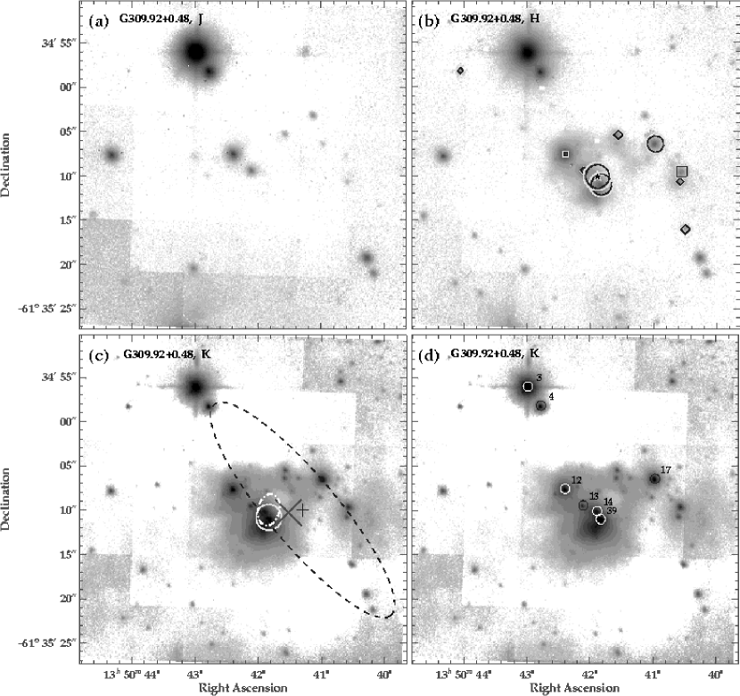
Figure 1: Near-IR images of G309.92+0.48. (a) J-band image. The grey-scale varies from 12.0 $\>\mathrm{mag/arcsec^{2}}$ (dark) to 20.5 $\>\mathrm{mag/arcsec^{2}}$ (white). The sharp-edged grey features in the background are artifacts from the mosaics and are shown to illustrate the noise level in the images. (b) $H$-band image. The grey-scale varies from 9.0 to 19.5 $\>\mathrm{mag/arcsec^{2}}$. The symbols represent stars whose $J-H$ and $H-K_{s}$ colours are above certain cut-off values (see Fig. 2 and explanation in Sec. 4.2.1). Stars with spectral types earlier than O3V are represented by open circles. Spectral types in the range O9V - O3V are represented by open squares. B9V - B0V types are represented by diamonds and A9V - A0V are represented by triangles (none appears in this figure). Pentagon-labelled stars (none appears in this figure) have spectral types later than A9V. The size of the symbols is proportional to the $H-K_{s}$ colour. Stars of any spectral type with intrinsic near-IR excess are labelled with a dark five-pointed star of fixed size. (c) $K$-band image. The grey-scale varies from 10.0 to 20.5 $\>\mathrm{mag/arcsec^{2}}$. The solid circle represents the radio emission at 3.6 cm from (Walsh et al., 1998). The plus symbol and the dashed ellipse represent the position and 1$\sigma$ positional error ellipse of the IRAS source. The MSX positional error ellipse (3$\sigma$) is plotted as a thick grey dot-dashed ellipse. The large thick cross indicates the position of the CS core from Bronfman et al. (1996). The cross size indicates the pointing error of the CS peak. (d) Some of the sources selected to produce the colour-colour and colour-magnitude diagrams of Figure 2 are labelled on the $K$-band image. In these and the following images shown in this paper, north is up and east is left.

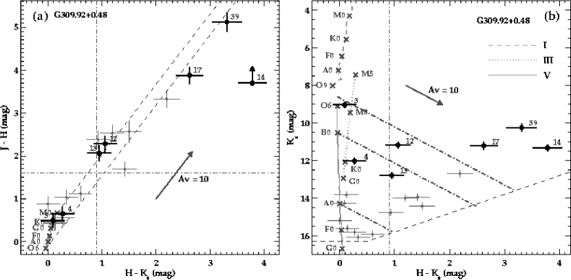
Figure 2: (a) Colour-colour diagram of G309.92+0.48. The grey solid line at the bottom left of the diagram represents the Main Sequence, where some spectral types are marked with crosses. The dashed lines show the reddened Main Sequence. The arrow represents a visual extinction of 10 mag. The colours of most of the sources in our images are represented by grey error bars. The colours of some selected sources (listed in Table 3 and labelled in Fig. 1) are represented by black circles with error bars. Some of these sources (#12, #13, #14, #17 and #39) have been selected because they are bright in the K band, they are located near the radio peak, and have considerable near-IR excess, which makes them the best candidates for ionizing sources of the UC H ii region. The remaining sources (#3 and #4) are bright in the 3 bands. They are normally bright nearby stars with hardly any extinction, and therefore, they should appear at the bottom left of the C-C diagram. Hence, they were selected to check for consistency in the photometry. These selection criteria for labelling are followed in all the remaining UC H iis shown in this paper. The arrow for source #14 indicates that it was not detected in the $J$ filter. The vertical and horizontal dot-dashed lines represent the $H-K_{s}$ and $J-H$ colour cut-offs between foreground stars and stars likely belonging to the UC H ii region (see discussion in Sec. 4.2.1). (b) Colour-magnitude diagram of G309.92+0.48 at a distance of 5.5 kpc. The unreddened Main Sequence is represented by the grey solid line. The dotted line is the giant branch and the grey-dashed line represents the super-giant branch. Spectral types are indicated by crosses along each branch. A reddening vector of 10 visual magnitudes is represented by a grey arrow. The dark dashed line is our detection limit. The colours of several sources measured in our near-IR images are represented with the same symbols as in panel (a). The vertical dot-dashed line represents the same $H-K_{s}$ colour cut-off as in panel (a). Dot-dashed lines parallel to the extinction arrow separate different spectral types. The upper of these lines corresponds to an spectral type O3V, whose $\mathrm{M_{v}}$ is 0.5 mag brighter than that of an O6V star (Vacca et al., 1996) and we assume to have the same intrinsic colours as an O6V star.

Figure 2 shows the colour-colour and colour-magnitude diagram of selected stars within the field of view of our near-IR images. We have labelled with numbers the some of the brightest stars in the K band. In particular, we have labelled those sources which are located near the UC H ii region, and which have considerable near-IR excess, since they are the best candidates for ionizing sources of the UC H ii region. Figure 2a indicates that two of the most obscured sources (#39 with A_v$\sim$60 mag, and #14 with A_v$>$50 mag) are located near the peak of the 3.5 cm emission. Source #39 lies within the extincted Main Sequence, while source #14 appears to show some IR excess. Source #17, which is located at 8^′′ (i.e. 0.2 pc at the adopted distance of 5.5 kpc) NE of the UC H ii region, is also highly extincted (A_v$\sim$45 mag). The extinction appears to be lower towards the NW of the UC H ii region, since sources #12 and #13 have visual extinctions of $\sim$ 25 mag.

The C-M diagram (Fig. 2b) is helpful to find out which of these sources are most likely to be responsible for the ionization of the UC H ii region. The C-M diagram indicates a spectral type either earlier than O6V or approximately K0I for source #39. However, if source #39 is a super-giant, its spectral type would be too cold (K0I) to ionize the H ii region, although it would contribute considerably to the total luminosity of the system. For source #14, a somewhat more uncertain spectral type $\sim$ O9I or earlier than O6V is estimated once its $H-K_{s}$ excess is removed from the C-M diagram, following the procedure described in Sec. 3.2.1. Source #14 could be a super-giant and still ionize the H ii region. Source #17 appears to be a reddened early OV or a late AI star, which in the later case, would be too cold to be candidate for ionizing source. The location of source #12 in the C-M diagram is consistent with an intermediate OV or KIII star under moderate extinction. Source #13 can be interpreted as a late O/early B Main-Sequence star or an early KIII star. Hence, if we discard the possibility that stars #12 and #13 are giants, and #17 and #39 are super-giants, we find up to 5 possible ionizing sources for the UC H ii region, one of which (#14) could still be a super-giant.

Once the main near-IR population has been analysed, we now focus on the radio and IRAS data for G309.92+0.48 (catalog

$$BE83$$

IR 309.92+00.48). A peak flux density of 350 mJy/beam at 3.5 cm (Walsh et al., 1998), a beam size of 1$\farcs$3 and a T${}_{\mathrm{e}}=7500$ K were utilised to calculate the beam temperature, optical depth, and emission measure, which yielded a log(N_L)=48.0 at a distance of 5.5 kpc. The stellar models from Smith et al. (2002) indicate a O9V spectral type for the ionizing source capable of producing such a Lyman photon rate. Any of the possible ionizing sources listed in the previous paragraph would suffice to produce such a Lyman photon rate. A total luminosity of $3.2\pm 0.2\times 10^{5}$ L_☉ was inferred from the fluxes of IRAS 13471-6120 given in the IRAS point source catalogue, which indicates an O5V spectral type for the heating source. Source #39 alone is already more luminous than the IRAS source. An anisotropic dust distribution in the UC H ii region or the presence of undetected (obscured) stars may account for this discrepancy between the IRAS luminosity and the luminosity of the observed near-IR stellar population (see the general discussion in Sec. 4.2.4).

4.1.2 G351.16+0.70 (catalog $$BE83$$ IR 351.16+00.70)(NGC 6334-V)

NGC 6334-V (catalog ) is a far-IR source (McBreen et al., 1979; Loughran et al., 1986) in the complex star forming region NGC 6334. In the original low-resolution map at 69 µm by McBreen et al. (1979), NGC 6334-V appears as a point source at a resolution of $\sim$3^′. The peak of NGC 6334-V is located 30^′′ towards the north of IRAS 17165-3554 (catalog ). Radio-interferometric studies (Simon et al., 1985; Rengarajan & Ho, 1996; Walsh et al., 1998; Jackson & Kraemer, 1999; Argon et al., 2000) revealed several compact (radii $<$ 2^′′) continuum sources, which are located 25^′′ towards the south/south-east of the far-IR peak. Using the VLA in C configuration, Jackson & Kraemer (1999) found that several of these compact sources are included in the southern rim of a large radio-shell of $\sim 1^{\prime}$ radius. The geometrical centre of the shell is offset $\sim 1^{\prime}$ to the NE of NGC 6334-V. The shell shows a clumpy morphology, which leaves the question open of whether the compact continuum sources are clumps in the shell or independent sites of star formation. Some of these compact radio sources are associated with water, OH (Braz & Epchtein, 1983; Argon et al., 2000) and methanol (Walsh et al., 1998) maser emission. A large-scale bipolar molecular outflow is also seen towards this star-forming region (Phillips & Mampaso, 1991).

NGC 6334-V has been extensively studied at near- and mid-IR wavelengths (Harvey & Gatley, 1983; Harvey & Wilking, 1984; Simon et al., 1985; Straw et al., 1989; Burton et al., 2000). Up to now, the highest spatial resolution in the near-IR ($\sim$3$\farcs$5) was achieved by Straw et al. (1989) and Burton et al. (2000).

In Figure 3, we present our AO-assisted images from ADONIS in the $J$, $H$ and $K$-bands, which have a resolution $\sim$25 times better than previous studies. In the field of view of our images, some of the unresolved sources from Straw et al. (1989) (labelled IRS 24, IRS 25, IRS 39) appear clearly resolved into several components. The bipolar reflection nebula studied by Harvey & Wilking (1984) and Simon et al. (1985) can be seen towards the south-west in our images. Both lobes (IRS 24 and IRS 25) are clearly separated from each other and composed of several knots. Both nebular lobes are located inside the positional error ellipse of IRAS 17165-3554.

No near-IR counterpart is detected at the position of the compact radio source detected by Argon et al. (2000) (solid ellipse in Fig. 3c), which is located between both lobes of the nebula. This compact source is also the radio source R-E3 detected by Rengarajan & Ho (1996) (lower right triangle in Fig. 3c). The 20 µm source from Harvey & Wilking (1984) (open square in Fig. 3c) has no near-IR counterpart either. The eastern lobe of the nebula coincides with the position of the radio continuum source R-E2 (Rengarajan & Ho, 1996; Jackson & Kraemer, 1999). The irregular UC H ii region detected by Walsh et al. (1998), with coordinates (J2000) $\alpha$=17^h19^m59$\fs$9, $\delta$=-35^∘57^′40^′′, is off the field of view of our images. The most interesting feature in our images is the group of $\lesssim 10$ unresolved near-IR sources at the position of the source IRS 39 (Straw et al., 1989), which is coincident with the far-IR peak, NGC 6334-V.

Our C-C diagram (Fig. 4a) indicates a reddening of 30 - 40 magnitudes in the visual at the location of NGC 6334-V. Source #45 (see Fig. 3d) is obscured by an A_v of $\sim$40 mag. Sources #33 and #36, located within 5^′′ of #45, follow in decreasing degree of obscuration, with visual extinctions $>$30 mag each. In the same association of unresolved IR sources, #46 appears to have a visual extinction of $\sim$20 mag. The extinction near the compact region R-E3 appears to be higher, since no near-IR point source is detected. Source #29, located at $3^{\prime\prime}$ to the east of R-E2, apparently has an extinction of $\sim$20 mag in the visual. However, this source is clearly extended in our $K$-band image, probably a knot in the nebula IRS 25, and hence the extinction determination is very uncertain.

The C-M diagram shown in Figure 4b yields further insights into the stellar population. Associated with the far-IR source NGC 6334-V, we identify one O6V (#45) star, and three BV stars (#33, #36 and #46). Note that the de-reddened colours of these four point sources are also consistent with spectral types in the early-to-mid MIII. In principle, this possibility cannot be discarded, except for the presumed youth of NGC 6334-V. In the same association, #34 appears to be barely extincted, indicating that this is likely a foreground star. In the inmediate surroundings of the R-E3 region no near-IR point source was detected, probably due to high extinction. This is supported by the presence of an MSX source located at the same position as RE-3.

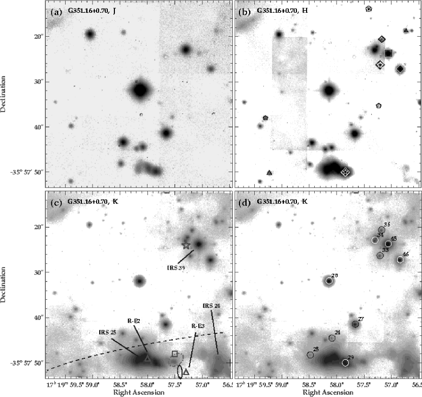
Figure 3: AO-assisted near-IR images of G351.16+0.70/NGC 6334-V taken with ADONIS at the 3.6m telescope in La Silla. (a) $J$-band image. The greyscale varies from 14.6 $\>\mathrm{mag/arcsec^{2}}$ (dark) to 20.3 $\>\mathrm{mag/arcsec^{2}}$ (white). (b) $H$-band image. The greyscale varies from 13.5 to 18.4 $\>\mathrm{mag/arcsec^{2}}$. See Fig. 1 for a key to the symbols. (c) $K$-band image. The greyscale varies from 9.8 to 18.9 $\>\mathrm{mag/arcsec^{2}}$. The small solid ellipse represents the 3.5 cm continuum emission from Argon et al. (2000). The triangles indicate the location of the radio-continuum sources R-E2 and R-E3 from Rengarajan & Ho (1996) (see also Jackson & Kraemer, 1999). The plus symbol and the dashed line represent the position and positional error ellipse of the IRAS source. The five-pointed star represents the central position of the far-IR source NGC 6334-V from McBreen et al. (1979). The open square indicates the location of the 20 µm source from Harvey & Wilking (1984). The near-IR sources IRS 24, 25 and 39 from Straw et al. (1989) are also indicated. The MSX source is represented by the dot-dashed small ellipse. No CS clump appears in the field of view. (d) Some of the sources selected to generate the colour-colour and colour-magnitude diagrams of Figure 4 are overlaid on the $K$-band image.

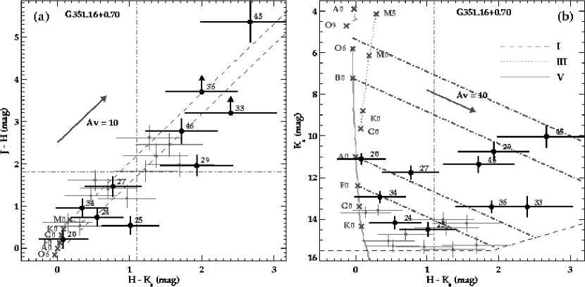
Figure 4: (a) Colour-colour and (b) colour-magnitude diagram for G351.16+0.70. Key to symbols and lines is given in Figure 2.

The large-scale shell, with a radius $\sim$0.3 pc, detected by Jackson & Kraemer (1999) at 3.5 cm, has an integrated flux density of 1.2 Jy. At a distance of 1.2 kpc, a log(N_L)=47.3 is needed to ionize the shell with a T${}_{\mathrm{e}}=7500$ K. If we compare this value with the predictions from the stellar models of Smith et al. (2002), the inferred spectral type for the ionizing star of the large scale shell is B0V. If the radio peaks R-E2 and R-E3 are considered to be independent UC H iis rather than clumps (with no stars inside) forming part of the large-scale shell, similar lower limits for the spectral types are inferred from their 3.5 cm flux (1.4 - 1.7 mJy; Jackson & Kraemer 1999). No near-IR point-like counterpart is found coincident with any of the compact radio sources.

We focus our attention on the compact association of near-IR point sources resolved at the position of IRS 39. We infer a spectral type for source #45 (O6V) which would produce more than enough Lyman photons to ionize the large-scale shell. Besides, sources #33, #36 and #46 (early BV spectral types) can also play a role in the ionization of the shell. However, the fact that this stellar association is located near the southern rim of the shell, rather than near the centre makes it quite unlikely that they are the main ionizing sources for the whole shell. If source #45 is contributing partially to the ionization of the southern rim of the shell, it is difficult to explain why no traces of ionized gas are seen at the position of source #45 itself. The possibility that #45, #33, #36 and #46 are protostars can be discarded, since they show low intrinsic $K$-band excess in our C-C diagram.

Two possible spectral types can be determined for the dust heating sources from the mid- and far-IR data available for G351.16+0.70 (catalog

$$BE83$$

IR 351.16+00.70). The first estimate is based on the fluxes from IRAS 17165-3554. A total luminosity of $4\pm 1\times 10^{4}$ L_☉ yields a spectral type for the heating source later than B0V (see Table 3.2.1). The second estimate is obtained by scaling the total luminosity given in Loughran et al. (1986) for the far-IR source NGC 6334-V ($1.7\times 10^{5}$ L_☉ at 1.7 kpc) to our assumed distance of 1.2 kpc. We obtain a new L_TOT=$8.5\times 10^{4}$ L_☉, which yields an O8V spectral type for the heating source.

The IRAS source is associated with the western lobe of the bipolar nebula (IRS 24). Since this is at the edge of the field of view of our images, we do not have photometric information on the stellar population to compare with the IRAS luminosity. The situation is different in the case of the far-IR source NGC 6334-V, which is clearly associated with the group of embedded near-IR sources #45, #33, #36 and #46 in our images. The spectral type inferred for the near-IR sources (one $<$O6V and three early-to-mid BV) is clearly earlier than the O9.5V needed to explain the total luminosity associated with NGC 6334-V. Therefore, these near-IR sources maybe contributing only partially to the heating of NGC 6334-V.

4.1.3 G5.89-0.39 (catalog GAL 005.89-00.39)

G5.89-0.39 (catalog GAL 005.89-00.39) was classified by Wood & Churchwell (1989) as a shell-type UC H ii region of diameter 5^′′. Kim & Koo (2001) found that the compact radio emission is located near the centre of a 15^′ extended ionized halo. Several OH, H₂O, and CH₃OH maser spots have been found in the region (Argon et al., 2000; Hofner & Churchwell, 1996; Walsh et al., 1998). G5.89-0.39 (catalog GAL 005.89-00.39) is known to be associated with an outflow, whose orientation has been found to be different (E-W,N-S,NE-SW) depending on the author and the tracer (Harvey & Forveille, 1988; Cesaroni et al., 1991; Acord et al., 1997; Sollins et al., 2004).

Near-IR images at the seeing limit were obtained by Harvey et al. (1994). A detailed study of this UC H ii region from near-IR to millimetre wavelengths was presented by Feldt et al. (1999). They show the first AO-assisted near-IR images of the region, with a resolution of 0$\farcs$4 in the $K$ band.

Our new high-resolution near-IR images of G5.89-0.39 (catalog GAL 005.89-00.39) taken with ALFA are presented in Figure 5. The resolution of these data is comparable to that shown in Feldt et al. (1999) (see also Henning et al., 2002). Our images show basically the same features as in Feldt et al. (1999). Nevertheless, we include them here for completeness.

The C-C diagram of this region is shown in Figure 6a (we use the same notation as in Feldt et al. 1999). Several sources appear to have $H-K_{s}$ excesses, although we focus our attention on sources #14, #16 #17 and #20, since they are very red and are located within or very close to the radio UC H ii region. Source #14 appears as an unresolved core surrounded by an extended halo in our ALFA $K_{s}$-band image, while source #16 is only barely resolved. Source #17 is unresolved and source #20 appears to be clearly extended. In any case, we tried to assign a spectral type to all of them, by using the method described in Sec. 3.2.1. Sources #14 and #17 appear to be late BV stars under $\sim$ 20 mag of visual extinction. The photometry of source #20 is consistent with a B5V star under a A_v $\sim$ 25 mag. Source #16 shows an extremely large excess, $H-K_{s}$ $\sim$ 4 mag, which yields a $\sim$ F5V spectral type, under the assumption that all the excess is in the $K_{s}$ band. In the cases of sources #14, #17, and #20, giant spectral types from KIII to GIII are also possible based only on the photometry, but then these stars would lack of any ionizing capabilities.

AO-assisted Fabry-Perot imaging shows that #14 and #20 are strong Br$\gamma$ emitters, which would explain part of their IR excess (Puga et al., 2004b). The same data indicate that part of the emission in #16 is also due to Br$\gamma$. Recent $K$- and $L^{\prime}$-band imaging with NAOS/CONICA at the VLT, with higher resolution and sensitivity that our ALFA images, indicate that source #16 actually contains a star of spectral type O5V (Feldt et al., 2003), which is likely to be the ionizing star of the UC H ii region due to its location within the shell. Hence, our assumption of all the $H-K_{s}$ excess coming from the $K_{s}$-band appears to yield a far too late (F5V) spectral type. Therefore, we adopt hereafter the spectral type inferred by Feldt et al. (2003), which scaled form their adopted distance of 1.9 kpc to our value of 2.6$\pm$0.6 kpc, is $\sim$ O3V.

The spectral type of the ionizing star inferred from radio data is O8V (see Table 3.2.1). The spectral type of a single star necessary to produce the IRAS emission is O7V. Hence, in G5.89-0.39 (catalog GAL 005.89-00.39), the near-IR spectral type of the best candidate for ionizing the H ii region is earlier than the radio and IRAS spectral type. This is a common feature of almost all UC H iis studied here, which will be discussed in Secs. 4.2.3 and 4.2.4.

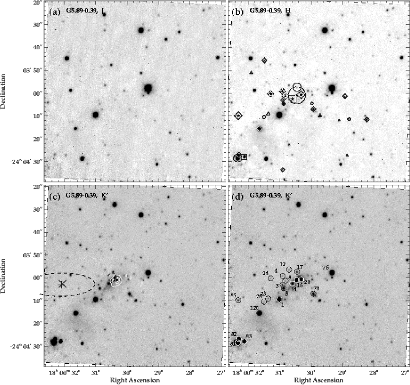
Figure 5: Near-IR images of G5.89-0.39. (a) $J$-band image. The greyscale varies from 14.5 $\>\mathrm{mag/arcsec^{2}}$ (dark) to 15.0 $\>\mathrm{mag/arcsec^{2}}$ (white). (b) $H$-band image. The greyscale varies from 12.8 to 13.0 $\>\mathrm{mag/arcsec^{2}}$. See Fig. 1 for a key to the symbols. (c) $K^{\prime}$-image. The greyscale varies from 10.06 to 10.14 $\>\mathrm{mag/arcsec^{2}}$. The white contours represent the radio-emission at 2 cm. Contour levels are at 5, 15 and 25$\sigma$. Symbols are the same as in Fig. 1. (d) Some of the stars selected to produce the colour-colour and colour-magnitude diagrams of Figure 6 are overlaid on the $K^{\prime}$-band image.

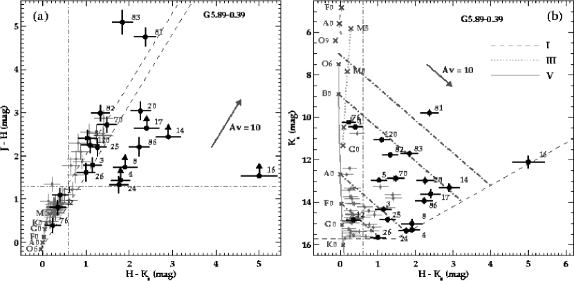
Figure 6: (a) Colour-colour and (b) colour-magnitude diagram for G5.89-0.39. Key to symbols and lines is given in Fig. 2.

4.1.4 G11.11-0.40 (catalog GAL 011.11-00.40)

This UC H ii region, which was classified as irregular by Kurtz et al. (1994), has a well-defined core at 3.6 cm, with a halo that extends 10^′′ towards the SE. It is associated with methanol maser emission (Walsh et al., 1997), and with high-velocity CO emission (Shepherd & Churchwell, 1996).

The near-IR data of G11.11-0.40 (catalog GAL 011.11-00.40) presented here form part of the previous work shown in Henning et al. (2001). Our new improved photometry – we use a more appropriate model for the PSF (see Sec. 2.5) and calibrate the photometry using the 2MASS PSC – yields $H$ and $K_{s}$ brightnesses 1 mag fainter than in Henning et al. (2001).

The near-IR morphology of this region is shown in Figure 7. We present the C-C and C-M diagrams in Figure 8. The most obscured sources within or near the radio-continuum emission are #8, #9, #12 and #22. Star #22, located some 10″ (0.25 pc) to the NE of the UC H ii region, also appears to suffer high extinction. The photometry of source #8 is consistent with an early AV star under a A_v $\sim$ 10 mag. Sources #9 and #22 are consistent with with late and early BV spectral types, respectively, with a visual extinction of $\sim$ 25 mag in both cases. Source #12, which is the closest to the radio peak, appears to be bluer than the reddened MS in the C-C diagram. The spectral type inferred from the C-M diagram is that of an O6V with a visual extinction of $\gtrsim 35$ mag. Note that in this case no correction for the near-IR excess was made.

From the 2 cm flux density listed in Kurtz et al. (1994), we infer a log(N_L)=47.8, i.e. a spectral type O9V for the ionizing source. This spectral type is later than the O6.8 ZAMS obtained by Henning et al. (2001) because they used the peak flux density to derive the electron density, and assumed this density to be uniform over a sphere of radius 0.2 pc. Here, we do the calculation using the integrated flux density within a sphere of 0.2 pc (Kurtz et al., 1994). The spectral type inferred from the IRAS fluxes is O9V, which is two spectral sub-types later that near-IR photometric spectral type of source #12. This UC H ii region represents one of the instances where the near-IR colours of the best candidate to be the ionizing star indicate a spectral type earlier than the one inferred from both radio and IRAS fluxes.

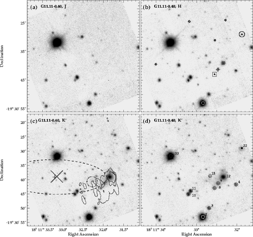
Figure 7: Near-IR images of G11.11-0.40. (a) $J$-band image. The greyscale varies from 13.5 $\>\mathrm{mag/arcsec^{2}}$ (dark) to 17.7 $\>\mathrm{mag/arcsec^{2}}$ (white). (b) $H$-band image. The greyscale varies from 13.0 to 17.9 $\>\mathrm{mag/arcsec^{2}}$. See Fig. 1 for a key to the symbols. (c) $K^{\prime}$-image. The greyscale varies from 12.4 to 17.2 $\>\mathrm{mag/arcsec^{2}}$. The contours represent the radio-emission at 3.6 cm. Contour levels are at 5, 15 and 25$\sigma$. Symbols are the same as in Fig. 1. (d) Some of the stars selected to produce the colour-colour and colour-magnitude diagrams of Figure 8 are overlaid on the $K^{\prime}$-band image.

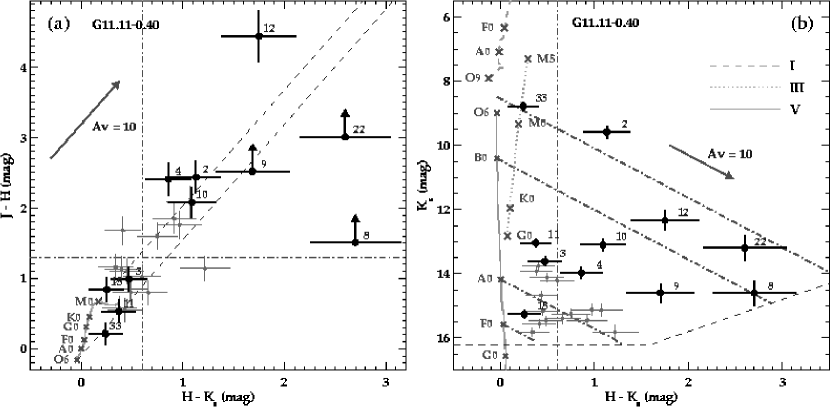
Figure 8: (a) Colour-colour and (b) colour-magnitude diagram for G11.11-0.40. Key to symbols and lines is given in Figure 2.

4.1.5 G18.15-0.28 (catalog GPSR5 18.147-0.284)

Little is known about this UC H ii region classified as cometary by Wood & Churchwell (1989). The radio source lies at the edge of a extinction lane that covers part of the eastern region in the FOV of our near-IR images (see Fig. 9). The C-C and C-M diagrams show that star #144, which is located within the radio UC H ii region, is the most obscured source. The C-C diagram indicates reddening towards this source due to pure extinction, with no intrinsic IR excess. The spectral type obtained from the C-M diagram is that of an O6V star under 30 magnitudes of visual extinction. Sources #143 and #121, with spectral types O7V and B0V and visual extinctions of 10 and 20 mag respectively, are also potential contributors to the ionization of the H ii region.

Kurtz et al. (1994) infer a log(N_L) = 46.8 from the integrated flux density at 3.6 cm, which implies an B0.5V spectral type for the ionizing source. Therefore in this case, it appears that the radio data underestimate by far the Lyman continuum photon rate associated to massive the stars detected with our near-IR photometry at and in the surroundings of the UC H ii region. The IRAS fluxes yield an O7V spectral type, which is in relatively good agreement with our near-IR photometry, unless we add up the luminosities from the brightest sources associated with the H ii region (#121, #143 and #144).

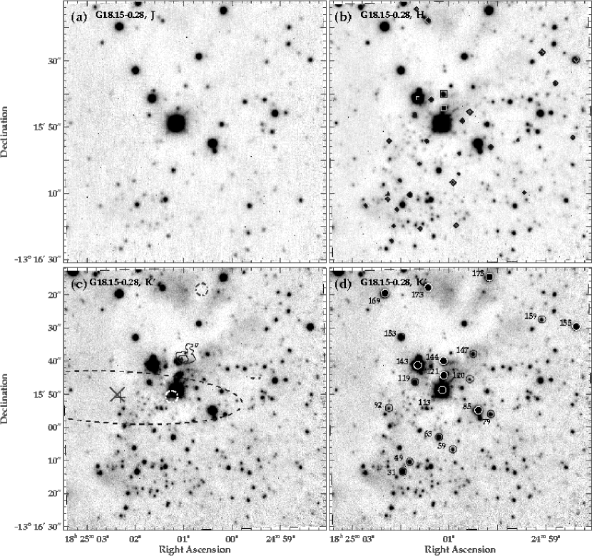
Figure 9: Near-IR images of G18.15-0.29. (a) $J$-band image. The greyscale varies from 14.8 $\>\mathrm{mag/arcsec^{2}}$ (dark) to 15.4 $\>\mathrm{mag/arcsec^{2}}$ (white). (b) $H$-band image. The greyscale varies from 13.6 to 13.9 $\>\mathrm{mag/arcsec^{2}}$. See Fig. 1 for a key to the symbols. (c) $K^{\prime}$-image. The greyscale varies from 11.10 to 11.14 $\>\mathrm{mag/arcsec^{2}}$. The contours represent the radio-emission at 3.6 cm. Contour levels are at 3, 6, 9 and 12$\sigma$. Symbols are the same as in Fig. 1. In this case, two MSX sources appear in the field of view (clear and dark small dot-dashed circles). (d) Some of the stars selected to produce the colour-colour and colour-magnitude diagrams of Figure 10 are overlaid on the $K^{\prime}$-band image.

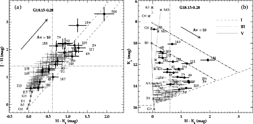
Figure 10: (a) Colour-colour and (b) colour-magnitude for G18.15-0.29. Key to symbols and lines is given in Figure 2.

4.1.6 G61.48+0.09 (catalog GAL 061.48+00.09)

G61.48+0.09 (catalog GAL 061.48+00.09) is a complex of two UC H iis located in the emission nebula Sh2-88B (Felli & Harten, 1981). Here, we focus our study on G61.48+0.09 (catalog GAL 061.48+00.09)B, which itself has two components (see Figure 11). B2 is the eastern region, classified as spherical or unresolved. B1, the western component, was classified as an extended cometary H ii region, which is undergoing a champagne flow (Garay et al., 1994, 1998a, 1998b). The presence of molecular gas associated with these H ii regions was inferred from CO and CS measurements (Schwartz et al., 1973; Blair et al., 1975). The velocity structure of the CO lines indicate the presence of several molecular outflows in G61.48+0.09 (catalog GAL 061.48+00.09) (Phillips & Mampaso, 1991; White & Fridlund, 1992).

This region has been previously studied in the near-IR by Evans et al. (1981) and Deharveng et al. (2000), the latter with a resolution comparable to our AO-assisted images. In a separate paper, we (Puga et al., 2004a) present a detailed description of this region, by combining AO-assisted near-IR polarimetry, narrow-band imaging and radio data with part of the photometry from this mini-catalogue.

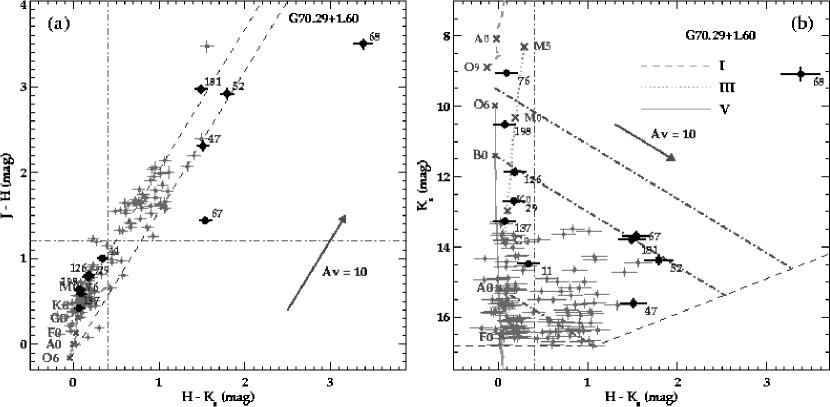
Figure 14: (a) Colour-colour and (b) colour-magnitude diagram of G70.29+1.60. Key to symbols and lines is given in Figure 2.

In Figure 14, we present our C-C and C-M diagrams for G61.48+0.09 (catalog GAL 061.48+00.09). There is some slight discrepancy between our magnitudes (see Table 3) and the data shown in Deharveng et al. (2000), although both sets of data agree within the errors. Stars #82 and #83 appear to be the main contributors to the ionization, due to their high luminosity, proximity to the radio peak and degree of obscuration. From our photometry, we infer an O9I spectral type for #82 and a B0V type for #83, under A_v’s of 35 and 15 mag, respectively. For this estimate, we have subtracted 0.2 mag from the $K_{s}$ magnitude of source #82 due to Br$\gamma$ emission (Puga et al., 2004a). The super-giant nature of star #82 is reinforced when its $L^{\prime}$ magnitude is also considered (Puga et al., 2004a).

The radio data yield different values for the number of Lyman continuum photon rate depending on which assumptions are made for the geometry of the radio-emitting region. In the case of the B2 component, if we scale the value of N_L given in Wood & Churchwell (1989) (log(N_L) = 46.2 at 2.0 kpc) to a distance of 2.7 kpc, we obtain a spectral type B1V for the ionizing source (see Table 3.2.1). For this estimate, Wood & Churchwell (1989) used the integrated flux and size at 6 cm measured with the VLA in B configuration. Deharveng et al. (2000), however, based their calculation on radio data taken at lower spatial resolution (Felli & Harten, 1981; Garay et al., 1993). They infer a log(N_L) = 48.4 and log(N_L) = 47.4 at a distance of 2.4 kpc for components B1 and B2, respectively. These Lyman photon rates scaled to a distance of 2.7 kpc imply spectral types for components B1 and B2 of $\sim$ O8V and $\sim$ B0V, respectively. Furthermore, Puga et al. (2004a) show that different (and equally valid) assumptions on the geometry of the ionized region, yield variations in the Lyman photon rate of up to one order of magnitude. The spectral type inferred from the IRAS source associated with G61.48+0.09 (catalog GAL 061.48+00.09) is an O7.5V.

Summing up, the spectral type for the hottest star derived from our near-IR photometry ($\sim$ O9I) is one luminosity class higher than the radio spectral type of component B1 ($\sim$ O9V) and also two spectral sub-types earlier than the radio spectral type of component B2 ($\sim$ B1V). An O9I star is 3.5 times more luminous than the luminosity inferred from the IRAS fluxes. This difference maybe explained if a population of stars hidden in our near-IR images are the actual ionizing sources of this complex H ii region, as well as the heating stars of the IRAS source. Part of this population may have already started to show up in recent $L^{\prime}$-band NACO observations (Puga et al., 2004a). An anisotropic dust distribution, which would be only partially heated by the detected near-IR population may also cause this difference.

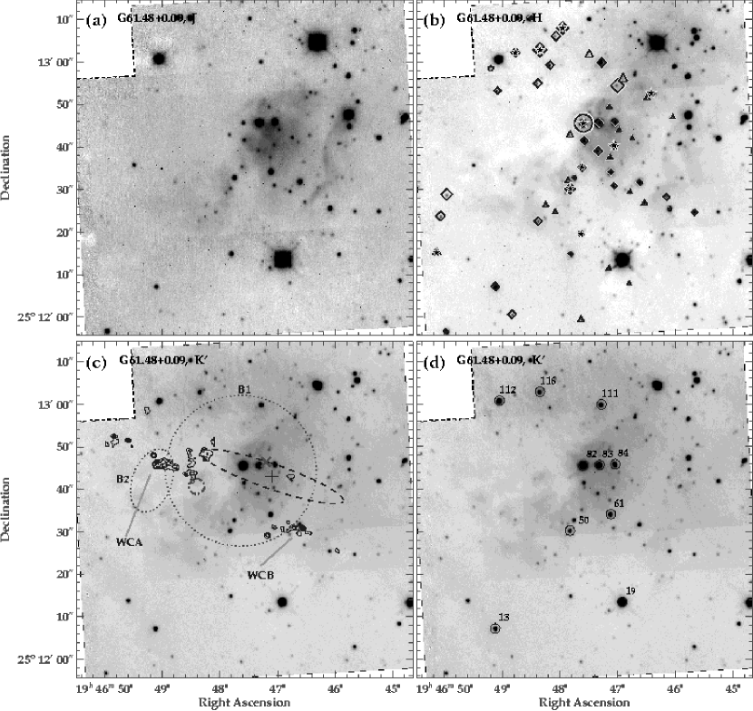
Figure 11: Near-IR images of G61.48+0.09. (a) $J$-band image. The greyscale varies from 14.8 $\>\mathrm{mag/arcsec^{2}}$ (dark) to 15.2 $\>\mathrm{mag/arcsec^{2}}$ (white). (b) $H$-band image. The greyscale varies from 13.3 to 13.6 $\>\mathrm{mag/arcsec^{2}}$. See Fig. 1 for a key to the symbols. (c) $K^{\prime}$-image. The greyscale varies from 10.60 to 11.72 $\>\mathrm{mag/arcsec^{2}}$. The contours represent the radio-emission at 6 cm with the VLA in B configuration (Wood & Churchwell, 1989). Contour levels are at 3, 6, 9, 12 and 15$\sigma$. The radio sources denominated G61.48+0.09A and B in Wood & Churchwell (1989) are here labelled as WCA and WCB, respectively. Symbols are the same as in Fig. 1. In addition, the two thin dotted ellipses represent the radio components B1 and B2 from Garay et al. (1993). (d) Stars selected to produce the colour-colour and colour-magnitude diagrams of Figure 12 are overlaid on the $K^{\prime}$-band image.

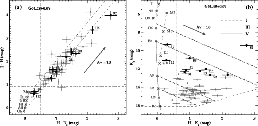
Figure 12: (a) Colour-colour and (b) colour-magnitude diagram for G61.48+0.09. Key to symbols and lines is given in Fig. 2.

4.1.7 G70.29+1.60 (catalog GAL 070.29+01.60) (K3-50A)

G70.29+1.60 (catalog GAL 070.29+01.60) is a well-studied UC H ii region, classified as a compact radio shell by Turner & Matthews (1984) and as a core-halo source by Kurtz et al. (1994). G70.29+1.60 (catalog GAL 070.29+01.60) is the brightest and youngest of a complex of 4 radio sources (K3-50A to D) spreaded over an area of 3$\farcm$5 (i.e. 8 pc at the adopted distance of 8.2 kpc). G70.29+1.60 (catalog GAL 070.29+01.60) is coincident with a 10 µm peak (Wynn-Williams et al., 1977), and also with a CS core (Bronfman et al., 1996).

Studies of radio-recombination line emission suggest the presence of moving ionized material (e.g. Rubin & Turner 1969; Wink et al. 1983; Roelfsema et al. 1988; DePree et al. 1994). In particular, DePree et al. (1994) show that G70.29+1.60 (catalog GAL 070.29+01.60) is undergoing a high-velocity bipolar outflow in the NW-SE direction. Based on CO observations, Phillips & Mampaso (1991) infer a bipolar outflow in the NE-SW direction.

Seeing-limited near-IR imaging was performed by Howard et al. (1996). They obtained an extinction map of the region as well as reinforced the idea of an outflow of ionized gas with a roughly north-south orientation. Okamoto et al. (2003) did a detailed study of the stellar population and ionization structure in the region, based on near- and mid-IR imaging and spectroscopy at a resolution of $\sim$ 0$\farcs$4 with the Subaru telescope. More recently, Hofmann et al. (2004) studied the morphology of the central $1^{\prime\prime}\times 1^{\prime\prime}$ with a resolution of $\sim$ 0$\farcs$1 using speckle imaging at the SAO 6 m telescope in Russia.

In Figure 13, we present our ALFA images of G70.29+1.60 (catalog GAL 070.29+01.60) with a resolution of 0$\farcs$22 and a Strehl ratio of 0.14 in the $K^{\prime}$-band. The morphology of the near-IR nebula is similar to that found by Okamoto et al. (2003) and Hofmann et al. (2004) (see the inset in Fig. 13c). Some of the sources labelled in Figure 13d (#29, #47, #52, #67 and #68) are clearly cross-identified with sources in Fig. 3 in Okamoto et al. (2003) and Figs. 1 and 2 in Hofmann et al. (2004). We also encounter near-IR point sources coincident with the position of the 11.4 µm peaks OKYM 3 and OKYM 4. In particular, our source #68 is coincident with OKYM 3, which is located at the centre of the radio-emitting source. No photometry of the near-IR source associated with OKYM 4 was possible, due to its location, which is highly embedded in the bright near-IR nebulosity.

Sources #67 and #68 are the most likely ionizing sources, based on their location with respect to the radio peak and their position in the C-C and C-M diagrams. Source #67 is consistent with a B0V star under a visual extinction of $\sim$ 20 mag. Detailed inspection of the $K^{\prime}$ band image shows that this source is elongated in the NW-SE direction. Source #68 appears to be extremely over-luminous in the C-M diagram. It has an excess of $\sim$ 1.5 mag in the $H-K_{s}$ colour. Even if we assume that this excess is mainly in the $K_{s}$ band, the high luminosity of source #68 can only be explained if it is a super-giant of spectral type later than A0I under $\sim$ 30 mag of visual extinction. However, due to the strong nebular contamination within the region of 2″ around #68, this spectral type estimate should be taken with caution. Besides, a star with such a spectral type would not contribute to the ionization of the H ii region. Further high-resolution spectroscopy in the near-IR is required to find photospheric lines associated with star #68, and therefore, to determine whether this source is actually a star, and if this where the case, to determine its spectral type.

In any case, we can compare the expected stellar ionizing population from published radio and IR data with the one suggested by our near-IR photometry. Kurtz et al. (1994) estimated a log(N_L)=49.3 and Martin-Hernandez et al. (2002) obtained a log(N_L)=49.1. If we scale these values to a distance of 8.2 kpc, we obtain an O5V spectral type for a single ionizing star (Smith et al., 2002). This value, based on 2 cm interferometry, is in good agreement with the O6V - O9V spectral type inferred by Okamoto et al. (2003) from modelling of the ionization structure of the mid-IR source OKYM 3 (i.e. our source #68). The Lyman photon rate of G70.29+1.60 (catalog GAL 070.29+01.60) (log(N_L) = 49.2) can also be produced by an O3I star, which would be in somehow better agreement with the luminosity inferred from our near-IR photometry. Regarding the other mid-IR source with near-IR counterpart (OKYM 4), Okamoto et al. (2003) obtained a spectral type between B0V and O9V. This source (star 10 in Hofmann et al., 2004) is not included in our C-C and C-M diagrams because it was barely detected in the $K^{\prime}$ image and not detected at all at shorter wavelengths.

Regarding the total luminosity of G70.29+1.60 (catalog GAL 070.29+01.60), its IRAS fluxes indicate a $\mathrm{\log(L/L_{\odot})}$ $\sim 6.30$. This cannot be delivered by a single dwarf star (note that $\mathrm{\log(L/L_{\odot})}$ = 6.03 for an O3V star), but it is plausible for a single super-giant star ($\mathrm{\log(L/L_{\odot})}$ = 6.27 for an O3I). Even source #68, which maybe an A9I star, would be not luminous enough. This maybe due to the presence of a population of hot stars, hidden at near-IR wavelengths, which would be contributing to the IRAS emission. Some members of this population could correspond to the mid-IR sources detected by Okamoto et al. (2003).

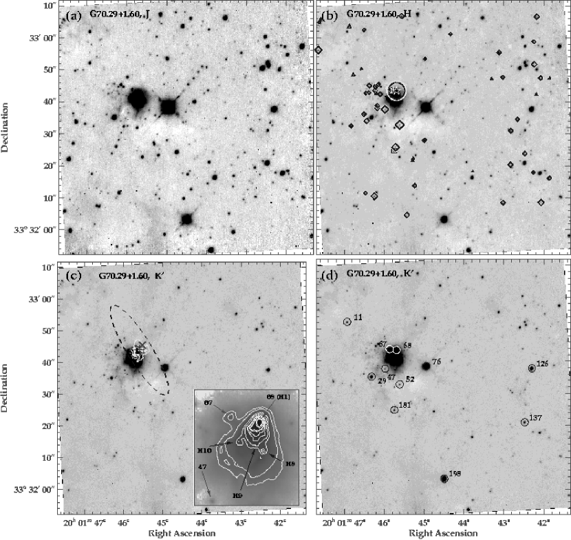
Figure 13: Near-IR images of G70.29+1.60. (a) $J$-band image. The greyscale varies from 14.5 $\>\mathrm{mag/arcsec^{2}}$ (dark) to 14.9 $\>\mathrm{mag/arcsec^{2}}$ (white). (b) $H$-band image. The greyscale varies from 13.2 to 13.8 $\>\mathrm{mag/arcsec^{2}}$. See Fig. 1 for a key to the symbols. (c) $K^{\prime}$-image. The greyscale varies from 10.6 to 10.8 $\>\mathrm{mag/arcsec^{2}}$. The contours represent the radio-emission at 2 cm. Contour levels are at 5, 15 and 25$\sigma$. Symbols are the same as in Fig. 1. In this case, the MSX source, the centre of the IRAS ellipse, and the CS core coincide within the errors. The inset shows a close up of the central 7$\farcs$5$\times$8$\farcs$5 of G70.29+1.60. A loglog scale was used to show both, the low level structure of the nebula as well as the point sources. Labels show some of the sources from Hofmann et al. (2004) (H1, H8, H9, H10) and some of the stars studied in our photometry. Note that H1 and H10 correspond with sources OKYM3 and OKYM4 in Okamoto et al. (2003), respectively. (d) Some of the stars selected to produce the colour-colour and colour-magnitude diagrams of Figure 14 are overlaid on the $K^{\prime}$-band image.

4.1.8 G77.96-0.01 (catalog GPSR 77.965-0.007)

This UC H ii region, located at a distance of 4.2 kpc from the Sun, was classified as irregular based on its morphology at radio wavelengths (Kurtz et al., 1994). Its sub-arcsecond morphology in the near-IR has not been previously studied.

In Figure 15, we present the ALFA $J$, $H$ and $K^{\prime}$ images of this region. The radio UC H ii region is coincident with a bright near-IR nebulosity in the north-eastern region of our FOV. Inspection of the 2MASS $K_{s}$ image over a field of view 5 times larger than the one shown in Figure 15 illustrates how the southern part of this reflection nebula is actually a bright knot of a long snake-like nebula extending for $\sim\,3^{\prime}$ towards the north-east and west.

Our C-C and C-M diagrams indicate two likely candidates which maybe ionizing the H ii region, sources #7 and #9, which are situated within 5″ (i.e. 0.1 pc) of the UC H ii region and within the near-IR nebulosity. They have spectral types $\sim$ O8V and B2V, respectively, both showing an extinction of about 10 magnitudes in the visual. At the location of the radio-peak, we find source #11. Its extinction is high enough to yield only an upper limit for the J magnitude. Its $H-K_{s}$ colour shows an excess of $\sim$ 1 mag. Its spectral type after removing, this excess is that of an early BV star. Another possibility is that this source may simply be an unresolved externally-ionized knot. Source #45 is also located within the near-IR nebulosity. The spectral type inferred for this source is O8V, with a visual extinction of 10 mag. Therefore, two O8V stars and two early BV stars appear to be the the best candidates for ionizing sources of this region.

We estimate a log(N_L) = 46.5 from the integrated flux and size of the G77.96-0.01 (catalog GPSR 77.965-0.007) radio source at 2 cm (Kurtz et al., 1994). This value implies a B1V spectral type for the ionizing source, which is later than the spectral types inferred from the near-IR photometry. For the IRAS source associated with G77.96-0.01 (catalog GPSR 77.965-0.007), we find a spectral type O8V, which is in good agreement with that of the hottest star in the near-IR images.

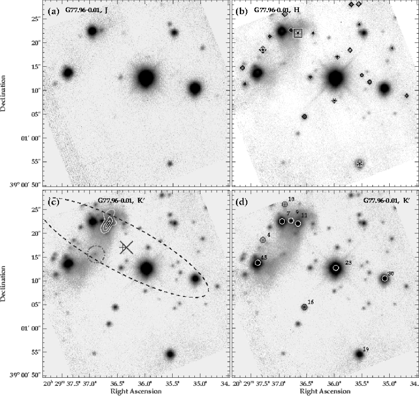
Figure 15: Near-IR images of G77.96-0.01 with a resolution of $0\farcs 5$. (a) $J$-band image. The greyscale varies from 13.4 $\>\mathrm{mag/arcsec^{2}}$ (dark) to 17.4 $\>\mathrm{mag/arcsec^{2}}$ (white). (b) $H$-band image. The greyscale varies from 12.8 to 17.4 $\>\mathrm{mag/arcsec^{2}}$. See Fig. 1 for a key to the symbols. (c) $K^{\prime}$-image. The greyscale varies from 11.9 to 16.8 $\>\mathrm{mag/arcsec^{2}}$. The contours represent the radio-emission at 3.6 cm. Contour levels are at 2, 6 and 9$\sigma$. Symbols are the same as in Fig. 1. (d) Some of the stars selected to produce the colour-colour and colour-magnitude diagrams of Figure 16 are overlaid on the $K^{\prime}$-band image.

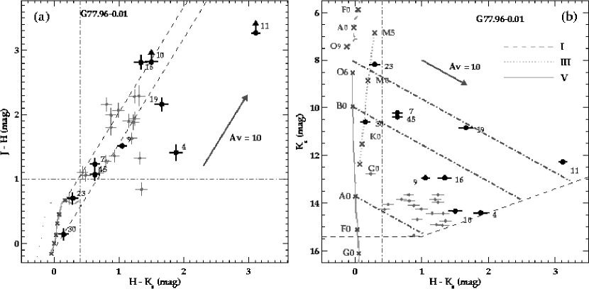
Figure 16: (a) Colour-colour and (b) colour-magnitude diagram of G77.96-0.01. Key to symbols and lines is given in Fig. 2.

4.2 General Properties

After having discussed each source individually, in this section we focus on the general features of our near-IR data, and compare them with published data at other wavelengths.

4.2.1 Mass Function

We note that all C-C diagrams show a gap in the distribution of stars along the band that represents the extincted MS. This gap appears to be clear in G70.29+1.60 (catalog GAL 070.29+01.60), but not so well defined in G18.15-0.28 (catalog GPSR5 18.147-0.284), where the photometric errors are larger. In any case, we have used this gap as a criterion to differentiate between foreground stars and stars which are likely to be associated with the H ii region. To quantify this distinction, we have defined two $J-H$ and $H-K_{s}$ colour cut-offs. Stars with colours above the cut-offs are assumed to be at the same distance as the UC H ii region. The spread of these stars along the extinction band in the C-C diagram is considered to be due to local variations of the dust and dense gas distribution at and in the surroundings of the H ii region. Colour cut-offs for each region are listed in Table 6 and are shown as dot-dashed lines in the C-C diagrams. In Table 6, the typical extinction towards stars above the cut-off is listed for each region. This typical extinction was estimated from visual inspection in the C-C diagram of the centroid of the stars along the reddened MS, which are also above the cut-offs. This value is slightly larger than the extinction associated to the point in the C-C diagram where both cut-off lines intersect. The expected line-of-sight foreground extinction to each source can be estimated from their distance. If we use A_v/d = 0.68 mag kpc^-1 from Bohlin et al. (1978) (where d is the distance), the expected foreground extinction ranges from 0.8 mag for G351.16+0.70 (catalog

$$BE83$$

IR 351.16+00.70) to 5.6 mag for G70.29+1.60 (catalog GAL 070.29+01.60). In all UC H iis, this foreground extinction is consistent with (i.e. smaller than) the A_v inferred from the colour cut-offs in our C-C diagrams.

From the C-M diagrams, we counted the number of stars for each spectral type located above the colour cut-offs, which we assume to be at the same distance as the UC H ii region. The star counts are shown in columns (4) to (8) of Table 6. For the lower end of the mass function, the completeness is clearly not reached, since MS stars later than A are normally below the detection limit. However, we can compare the ratio of the number of O-type stars to the number of B-type stars ($\mathrm{N_{O/B}}$), with the expected ratio from a theoretical expression for the IMF, since the completeness should be better in the upper end of the mass spectrum. In this mass range, the exponent of the IMF is -1.3 (Miller & Scalo, 1979), yielding a ratio $\mathrm{N_{O/B}}$$\sim 0.16$. For the regions that have high stellar counts, i.e. G18.15-0.28 (catalog GPSR5 18.147-0.284), G61.48+0.09 (catalog GAL 061.48+00.09) and G70.29+1.60 (catalog GAL 070.29+01.60), the $\mathrm{N_{O/B}}$ is 0.11, 0.03 and 0.07 respectively. The agreement between these values and the IMF is reasonably good for G18.15-0.28 (catalog GPSR5 18.147-0.284), but fails for G61.48+0.09 (catalog GAL 061.48+00.09) and G70.29+1.60 (catalog GAL 070.29+01.60). This maybe an indication that not all UC H ii regions contain very massive O stars. However, before any robust conclusion on the IMF can be drawn, deeper observations at higher resolution and also at longer wavelengths are needed to achieve a higher degree of completeness and to unveil very obscured stars.

Table 6: Star Counts

Object	$(H-K_{s})_{c}$	$(J-H)_{c}$	$>$O3V	O3V-O9V	B0V-B9V	A0V-A9V	$<$A9V	Ex.	Av
	mag	mag	#	#	#	#	#	#	mag
G309.92+0.48 (catalog $$BE83$$ IR 309.92+00.48)	0.9	1.6	3	2	5	$\cdots$	$\cdots$	1	16
G351.16+0.70 (catalog $$BE83$$ IR 351.16+00.70)	1.1	1.8	0	1	4	2	3	3	19
G5.89-0.39 (catalog GAL 005.89-00.39)	0.6	1.3	2	2	14	6	3	7	17
G11.11-0.40 (catalog GAL 011.11-00.40)	0.6	1.3	2	2	7	0	$\cdots$	3	16
G18.15-0.28 (catalog GPSR5 18.147-0.284)	0.6	1.4	0	3	27	2	$\cdots$	0	12
G61.48+0.09 (catalog GAL 061.48+00.09)	0.5	0.9	1	0	30	20	2	10	15
G70.29+1.60 (catalog GAL 070.29+01.60)	0.4	1.2	1	2	41	10	$\cdots$	2	14
G77.96-0.01 (catalog GPSR 77.965-0.007)	0.4	1.0	0	4	20	0	$\cdots$	6	14

4.2.2 Near-IR Ionizing Sources

We have made an attempt to identify, using near-IR photometry, the main ionizing stars for each UC H ii region. Column (3) of Table 3.2.1 shows that for all regions we have found at least one source with a spectral type early enough to be capable of ionizing an H ii region. However, the question of whether this source(s) is the actual ionizing star(s) of the radio UC H ii region is still to be answered. Our identification has the advantage of the high resolution delivered by AO imaging and the relative transparency of dust and dense gas at near-IR wavelengths. It is certainly true that these sources identified as ionizing stars are unresolved and show high extinction (A_v$>$30 mag) and/or intrinsic IR excess, which indicate their youth and possible relation with the H ii region. In all cases but G351.16+0.70 (catalog

$$BE83$$

IR 351.16+00.70) and G61.48+0.09 (catalog GAL 061.48+00.09), their position coincides with that of the radio peak which defines the UC H ii region (see H-band images in Figs. 1 to 15). Even the two exceptions can be explained. G351.16+0.70 (catalog

$$BE83$$

IR 351.16+00.70) appears to be simply a knot which is part of a much larger ionization shell ($1^{\prime}$ radius, i.e 0.4 pc), so it is not surprising that no stars are found at the radio peak. G61.48+0.09 (catalog GAL 061.48+00.09) appears to be a rather evolved compact H ii region, which shows several separated peaks at high-interferometric resolution and extends for over 30^′′ (i.e. 0.4 pc) in low-resolution radio maps.

We have used C-C and C-M diagrams to spectral-classify the possible ionizing sources and other sources associated with the UC H ii regions. Our photometric spectral classification, however, is not without problems. UC H ii regions appear to be rather complex in the near-IR at sub-arcsecond scales, showing some degree of crowdness as well as spatially variable background due to the presence of extended nebulosity. This makes it difficult to calculate magnitudes accurately. To solve at least partially these problems, we have used PSF fitting photometry, which should reduce the contribution to the stellar flux due to barely resolved stellar neighbours and due to the presence of a spatially variable background. The possibility that some of the sources identified as single stars are multiple systems or unresolved emission line knots cannot be completely discarded due to the relatively large distances (between 1.2 and 8.2 kpc) to these UC H ii regions. The high resolution delivered by AO though (between 0$\farcs$13 and 0$\farcs$55, which turns into projected separations of $\sim\,1000$ AU), alleviates this possibility. Other typical problems associated with the photometric spectral classification are temporal variability in young stars, undetermined photometric excesses due to unresolved dust emission, scattering, accretion discs, and uncertainties in the distance and in the extinction.

4.2.3 Comparison with Radio Sources

In most of the UC H iis, the spectral type of the ionizing source obtained from radio-continuum interferometry is a few sub-types later than the spectral type inferred from our near-IR photometry. One possible explanation is that part of the ionizing flux produced by the sources detected in our near-IR images is being absorbed by dust in the region. If the radio free-free emission is optically thick, radio interferometry may also be underestimating the Lyman continuum. A clumpy density distribution within the UC H ii region can also yield an underestimate for the N_L. One additional problem is the fact that radio interferometry is sensitive only to high spatial frequencies. If the UC H ii region is a mere density enhancement within a larger undetected extended halo of ionized gas, the total N_L associated with the full-size H ii region may be more compatible with the stellar content inferred from our near-IR photometry. Extended halos of ionized gas are known to exist in a number of UC H iis (e.g. Kurtz et al. 1999; Kim & Koo 2001). Kim & Koo (2001) find typical ratios $\gtrsim 10$ between H i 21 cm single dish fluxes and VLA fluxes. Even though the higher continuum flux in the single-dish observations comes from a larger ionized gas volume, the spectral types inferred from single-dish observations are 4 times earlier than those inferred from radio-interferometry. Such kind of differences would help to reconcile the spectral types inferred from the near-IR stellar population with those inferred from radio measurements.

A spectral type classification based on radio data also has the problem that it depends on the stellar models adopted. Table 3.2.1 shows that for a given N_L, the spectral types inferred using the models in Smith et al. (2002) are earlier than the spectral types inferred from the models in Vacca et al. (1996). This is mainly due to the more realistic approach of Smith et al. (2002), by using models that include stellar winds, spherical geometry, and line blanketing by metals (Pauldrach et al., 2001). Even though the line blanketing does not affect the N_L – $\mathrm{T_{eff}}$ relation (see Mokiem et al., 2004), it does affect the $\mathrm{T_{eff}}$ – spectral type relation. This trend towards earlier spectral types for a given $\mathrm{T_{eff}}$ is also seen when the CMFGEN models (Hillier & Miller, 1998), which also include stellar winds and line blanketing, are used (see Martins et al., 2002). Therefore, the use of models including a more realistic physics helps to reconcile the near-IR photometric spectral-type classification of the possible ionizing stars and the classification inferred from radio continuum measurements.

4.2.4 Comparison with IRAS Sources

We find that, in general, the luminosity inferred from the IRAS sources associated with the UC H iis is lower than what it is expected from the analysis of the stellar population based on our near-IR photometry (see Table 3.2.1). The spectral classification based on the luminosity inferred from IRAS fluxes is also model dependent. In this case, Table 3.2.1 shows that for a given L_TOT, the model grid by Smith et al. (2002) yields earlier spectral types slightly earlier than the grid by Vacca et al. (1996). This difference, even if it is only of half to one spectral sub-class, tends to reconcile the IRAS-based and photometric spectral types. In any case, even with the use of the grid by Smith et al., a discrepancy of over one spectral sub-class still exists between the IRAS and near-IR spectral types for most of the sources.

One possible explanation for this general discrepancy between IRAS and near-IR luminosities is that the stellar population that shows up at near-IR wavelengths is already in a rather advanced evolutionary stage, and therefore it is not the major contributor to the mid- and far-IR flux. It is likely that a more embedded population of stars which would show up at longer wavelengths is actually producing the majority of the mid- and far-IR flux. This maybe the case in G61.48+0.09 (catalog GAL 061.48+00.09) and G70.29+1.60 (catalog GAL 070.29+01.60), where studies at wavelengths longer than 2 µm appear to show part of this population (Puga et al., 2004a and Okamoto et al., 2003, respectively). AO-assisted observations with 8m-class telescopes at wavelengths longer than 2.2 µm  can provide the sensitivity and resolution necessary to pinpoint this possible embedded stellar population (see Feldt et al., 2003).

Alternatively, if the dust spatial distribution is anisotropic, it is possible that the stars seen in the near-IR are actually heating, but only partially, the dust producing the emission detected in the mid- and far-IR by IRAS. The radiation field associated with the IRAS source in this case will no longer be spherically symmetric, making luminosity estimates based on reprocessed radiation extremely geometry dependant. Stellar radiation will leak-out and leave no sign at mid- and far-IR wavelengths, yielding luminosities associated to the IRAS source smaller than those associated to the near-IR population.

A very simple calculation by dividing the luminosities inferred from the IRAS fluxes and the luminosities associated with the spectral types inferred from our near-IR photometry can be used to obtain a rough estimate of the fraction of radiation that must be absorbed by the dust causing the IRAS emission. We find that the fraction of absorbed radiation varies from only 10% for G351.16+0.70 (catalog

$$BE83$$

IR 351.16+00.70) to as high as $\sim$ 85% for G309.92+0.48 (catalog

$$BE83$$

IR 309.92+00.48). It is $\sim$ 25% for G5.89-0.39 (catalog GAL 005.89-00.39), G11.11-0.40 (catalog GAL 011.11-00.40) and G61.48+0.09 (catalog GAL 061.48+00.09)B1, and between 55% and 65% for G77.96-0.01 (catalog GPSR 77.965-0.007) and G18.15-0.28 (catalog GPSR5 18.147-0.284). For G70.29+1.60 (catalog GAL 070.29+01.60), the IRAS luminosity is higher than the near-IR luminosity. Interferometry in the mm and sub-mm range to trace the distribution of dust at a similar resolution to that of near-IR imaging, complemented with radiative transfer modelling will be necessary to further investigate this calculation.

4.2.5 CS Cores and MSX Sources

All UC H iis but G351.16+0.70 (catalog

$$BE83$$

IR 351.16+00.70) are associated with a CS core listed in Bronfman et al. (1996). Their position accuracy is $\sim\,3^{\prime\prime}$. Bronfman et al. (1996) observed these dense clumps in the millimetre CS(2-1) transition. They have sizes slightly higher than their instrumental beam size of $40^{\prime\prime}-50^{\prime\prime}$. The centroids of the CS cores are normally coincident with the IRAS peaks. The typical separation between the near-IR ionizing stars and the CS cores is between 7^′′ and 24^′′ (0.1 pc to 0.45 pc, in terms of physical distances), with the exception of G70.29+1.60 (catalog GAL 070.29+01.60), for which the separation is below 1^′′ (i.e. below 8000 AU). If the detected near-IR massive stellar population is contributing to the heating and stirring up (e.g. due to stellar winds) of the CS cores, one may expect some correlation between the near-IR spectral type and the brightness and velocity dispersion of the CS emission. We do not find such a correlation. The brightest CS core, with a mean beam temperature ($\mathrm{T_{mb}}$) of 5.6 K (Bronfman et al., 1996), is associated with G5.89-0.39 (catalog GAL 005.89-00.39). However, this dense core is rather far away ($\sim$ 0.3 pc) from the main near-IR ionizing star (and also from the radio-peak of the UC H ii region). In contrast, the near-IR ionizing star(s) of G70.29+1.60 (catalog GAL 070.29+01.60), whose associated CS core has a relatively low $\mathrm{T_{mb}}$ (1.95 K), are coincident with the centroid of the CS emission. We note that the two cores with the broader CS(2-1) profiles are associated with G5.89-0.39 (catalog GAL 005.89-00.39) and G70.29+1.60 (catalog GAL 070.29+01.60), which are known to be strong outflow sources.

We also made an attempt to correlate the properties of the MSX sources associated with the UC H ii regions in our sample, and the near-IR population. Inspection of our images shows that the centres of the MSX peaks are closer to the location of the radio UC H ii regions than the CS cores and IRAS sources. In column (9) of Table 3.2.1, we show the luminosity associated with the MSX sources. This luminosity was calculated by integrating a black body fit using only the fluxes at 14.65 µm and 21.34 µm (see Sec. 3.3), respectively. We find no correlation between the luminosity of the MSX source and the luminosity of the near-IR ionizing population.

4.2.6 Possible Super-giants?

We note that in 3 of the regions (G309.92+0.48 (catalog

$$BE83$$

IR 309.92+00.48), G61.48+0.09 (catalog GAL 061.48+00.09)B1 and G70.29+1.60 (catalog GAL 070.29+01.60)) the most luminous identified sources have near-IR colours consistent with being super-giants, rather than dwarfs. In the case of the regions G309.92+0.48 (catalog

$$BE83$$

IR 309.92+00.48) and G61.48+0.09 (catalog GAL 061.48+00.09)B1, these stars appear to have spectral types early enough as to be responsible for the ionization of the H ii region. A caveat should be pointed out here, since these high-luminosity sources may as well be mere unresolved ionized knots externally illuminated by other stars, rather than actual stars. Note that for instance, an ionized knot emitting purely in Br$\gamma$ may appear as a strong continuum source in the broad-band $K_{s}$ filter. If they are actually stars, their large absolute magnitude in K band (M_K) would be likely to be generated by a single star, since it cannot be explained as due to an unresolved multiple system formed by two or more stars. To prove this, we analyse the most exteme case, i.e. two O3V stars being misinterpreted as an O9.5I star. The visual magnitude (M_v) and intrinsic colours for an O9.5I star and an 03V star are such that M_K(O9.5I) =-5.65 mag and M_K(O3V) =-4.79 mag, respectively (Vacca et al., 1996; Aller et al., 1982). An unresolved binary composed of two O3V stars would have a total M_K=-5.24 mag, which is still 0.4 mag fainter than an O9.5I star. This difference is larger than the typical error in our photometry. Nevertheless, this argument cannot be used to discard possible triple and multiple systems of dwarfs. In one particular case (G61.48+0.09 (catalog GAL 061.48+00.09)) further Br$\gamma$ and $L^{\prime}$ imaging strongly supports the interpretation of the most luminous source being a super-giant rather than a dwarf (Puga et al., 2004a).

Although further near-IR spectroscopy is required to confirm the nature of these high-luminosity sources (Kaper et al., 2002), we can argue whether, in terms of evolution, the presence of a super-giant in these H ii regions is plausible. We use Eq. (9) from Wood & Churchwell (1989), with a typical value for the initial radius of the Strömgren sphere of 0.02 pc and a typical sound speed of 10 $\>\mathrm{\>km~{}s^{-1}}$. If we take into account the physical radius of G61.48+0.09 (catalog GAL 061.48+00.09)B1, G70.29+1.60 (catalog GAL 070.29+01.60) and G309.92+0.48 (catalog

$$BE83$$

IR 309.92+00.48), i.e. 0.18 pc, 0.14 pc and 0.03 pc respectively, then the ages of these H ii regions are $5\times 10^{4}$, $2.5\times 10^{4}$ and $1.1\times 10^{3}$ years, respectively. This is between 2 and 3 orders of magnitude shorter than the typical time of $\lesssim 10^{6}$ yr required for a 40 M_☉ star to reach the super-giant phase (Schaerer & de Koter, 1997).

Several arguments can be used to re-concile the presence of super-giants in some of the UC H ii regions. One may think that these luminous stars do not belong to the UC H ii region, but that they are foreground stars situated at the position of the radio peak by chance allignments. This is rather unlikely though, since they tend to be the most embedded sources in our C-C diagram. Besides, even though our sample is rather small, we find possible ionizing super-giants in 25% of the cases, which is difficult to explain simply by chance alignments. The presence of super-giants could be explained if the H ii regions were actually in a more advanced evolutionary stage than what is inferred from their physical size. This maybe the case if radio single-beam observations (or low resolution interferometry) of the ionized gas showed the presence of extended halos associated with these UC H ii regions. However, in instances as G61.48+0.09 (catalog GAL 061.48+00.09), even with a low-resolution configuration of the VLA, the 3.6 cm emission extends only for 0.18 pc. The external pressure due to the molecular cloud in which UC H iis are normally embedded may delay the expansion of the ionization front, yielding also older ages than what is predicted by simple expansion models. This argument has already been used before to explain the paradigm of the UC H iis lifetime (Wood & Churchwell, 1989). Tan & McKee (2004) show that an H ii region will expand to a given size in a timescale 2 orders of magnitude slower in a clumpy turbulent medium than in a uniform medium.

5 CONCLUSIONS

We have analized AO-assisted $J$, $H$ and $K/K^{\prime}$ band images and photometry of 8 UC H ii regions. These data show details of the near-IR morphology and stellar population in these regions with unprecedented spatial resolution. We have analized the stellar population using near-IR photometry. We find that the typical spectral types obtained from near-IR photometry are earlier than those predicted from radio-continuum interferometric data available in the literature. The possible underestimate of the rate of Lyman photons from radio data due to absorption by dust, optical depth effects, clumpiness or the presence of undetected extended ionized halos may be causing this difference. We have also compared the ionizing and luminous near-IR stellar population with the luminosity of the IRAS source associated with each UC H ii region. In general, we find that IRAS fluxes yield later spectral types for the dust heating source than near-IR photometry. This maybe due to the presence of a more embedded stellar population than the one accessible with near-IR photometry. This hidden population would be the main contributor to the IRAS luminosity. Alternatively, if the dust distribution is anisotropic, the stars seen in the near-IR may actually be heating the dust seen by IRAS. Stellar models with spherical geometry and a detailed treatment of stellar winds and line blanketing yield radio- and IRAS-based spectral types that are generally in better agreement with photometry-based spectral types than non-LTE, plane-parallel models.

In all cases, the C-C diagrams for these regions show two groups of stars. We assume that one of them, close to the unreddened theoretical Main Sequence, is formed by foreground stars. The stars in the other one normally show a large spread in extinction, and they are certainly associated with the UC H ii region. In all regions, we find at least one source with a spectral type early enough to be the ionizing star of the H ii region, i.e. early B/O. We have counted, in spectral-type bins, all stars associated with each UC H ii region. For G18.15-0.28 (catalog GPSR5 18.147-0.284), where we have a relatively high nuber of stars, a reasonable agreement is found between the observed O and B star numbers and those predicted by the IMF given in Miller & Scalo (1979). However, this is not the case for G61.48+0.09 (catalog GAL 061.48+00.09) and G70.29+1.60 (catalog GAL 070.29+01.60). For the remaining UC H iis, not enough stellar counts were available to make any estimate.

We have also compared the luminosity of the near-IR ionizing stellar population with MSX luminosities and no correlation was found. Our near-IR data were compared with available millimetre CS data to find out what is the impact the massive stellar population in UC H iis has on the surrounding dense gas. No correlation was found between the brightness of the CS emission and the luminosity of the best near-IR candidates to ionize the UC H ii region. We note that the velocity dispersion is larger in the CS cores in the G5.89-0.39 (catalog GAL 005.89-00.39) and G77.96-0.01 (catalog GPSR 77.965-0.007) regions, which are known to be associated with massive outflows.

In 3 regions (G61.48+0.09 (catalog GAL 061.48+00.09)B1, G70.29+1.60 (catalog GAL 070.29+01.60) and G309.92+0.48 (catalog

$$BE83$$

IR 309.92+00.48)), the most luminous stars in the UC H ii region appear to be super-giants. In G61.48+0.09 (catalog GAL 061.48+00.09)B1 and G309.92+0.48 (catalog

$$BE83$$

IR 309.92+00.48), these luminous stars are also the best candidates for ionizing sources of the H ii region.

The main conclusion from this work is that AO-assisted near-IR imaging of UC H iis with 4m-class telescopes is a useful tool to study the stellar population in massive star-forming regions. This appears to be a more accurate method to study the massive young stellar population than any indirect method based on radio, IRAS or MSX measurements, mainly due to the higher resolution provided by AO observations. Nevertheless, it is also fundamental to observe at longer wavelengths (from 3.5 µm to 20 µm) with similar spatial resolution in order to detect the most embedded stellar population. Deeper observations are necessary to achieve a better coverage of the IMF. Finally, broad-band imaging should be complemented with near-IR spectroscopy and narrow-band imaging to fully understand the nature of the relevant stellar population in each region. AO imaging at 8m-class telescopes is a promising tool to achieve these goals.

References

- Acord et al. (1997) Acord, J. M., Walmsley, C. M., & Churchwell, E. 1997, ApJ, 475, 693
- Afflerbach et al. (1996) Afflerbach, A., Churchwell, E., Acord, J. M., et al. 1996, ApJS, 106, 423
- Aller et al. (1982) Aller, L. H., Appenzeller, I., Baschek, B., et al. 1982, Landolt-Börnstein: Numerical Data and Functional Relationships in Science and Technology, p451
- Argon et al. (2000) Argon, A. L., Reid, M. J., & Menten, K. M. 2000, ApJS, 129, 159
- Behrend & Maeder (2001) Behrend, R. & Maeder, A. 2001, A&A, 373, 190
- Beuzit et al. (1994) Beuzit, J., Hubin, N., Gendron, E., Demailly, L., et al. 1994, SPIE, 2201, 955
- Blair et al. (1975) Blair, G.N., Peters & van den Bout, P. A. 1975, ApJ, 200, L61
- Blitz et al. (1982) Blitz, L., Fich, M. & Stark, A. A. 1982, ApJS, 49, 183
- Bonnell et al. (1998) Bonnell I. A., Bate M. R., Zinnecker H. 1998, MNRAS, 298, 93
- Bohlin et al. (1978) Bohlin, R. C., Savage, B. D., & Drake, J. F. 1978, ApJ, 224, 132
- Braz & Epchtein (1983) Braz, M. A. & Epchtein, N. 1983, A&AS, 54, 167
- Bronfman et al. (1996) Bronfman, L., Nyman, L.-A., & May, J. 1996, 115, 81
- Burton et al. (2000) Burton, M. G., Ashley, M. C. B., Marks, R. D., et al. 2000, ApJ, 542, 359
- Cesaroni et al. (1991) Cesaroni, R., Walmsley, C. M., & Kömpe, C., et al. 1991, A&A, 252, 278
- Churchwell et al. (1978) Churchwell, E., Smith, L. F., & Mathis, J., et al. 1978, A&A, 70, 719
- Crowther & Dessart (1998) Crowther, P. A. & Dessart, L. 1998, MNRAS, 296, 622
- Crowther (1998) Crowther, P. A. 1998, The effective temperatures of hots stars, IAU Symp. 189: Fundamental Stellar Properties, 137
- Crowther & Conti (2003) Crowther, P. & Conti, P. S. 2003, MNRAS, 343, 143
- Cutri et al. (2003) Cutri, R. M., Skrutskie, M. F., van Dyk, S., Beichman, C. A., Carpenter, J. M. et al. 2003, 2MASS All-Sky Catalog of Point Sources, VizieR, II/246
- Deharveng et al. (2000) Deharveng, L., Nadeau, D., Zavagno, A., et al. 2000, A&A, 360, 1107
- DePree et al. (1994) DePree, C. G., Goss, W. M., Palmer, P., et al. 1984, ApJ, 428, 670
- Ducati et al. (2001) Ducati, J. R., Bevilacqua, C. M., Rembold, S. B., & Ribeiro, D. 2001, ApJ, 558, 309
- Egan et al. (2003) Egan, M. P., Price, S. D., Kraemer, K. E., & Mizuno, D. R., et al 2003, MSX6C Infrared Point Source Catalog, VizieR, V/114
- Epchtein & Lepine (1981) Epchtein, N. & Lepine, J. R. D. 1981, A&A, 99, 210
- Epchtein et al. (1981) Epchtein, N., Guibert, J., Rieu, N. Q., et al. 1981, A&A, 97, 1
- Evans et al. (1981) Evans, N. J., Harvey, P., Israel, F., et al. 1981, ApJ, 250, 200
- Feldt et al. (1998) Feldt M., Stecklum B., Henning Th., Hayward T. L., Lehmann T., & Klein R. 1998, A&A, 339, 759
- Feldt et al. (1999) Feldt, M., Stecklum, B., Henning, Th., et al. 1999, A&A, 346, 243
- Feldt et al. (2003) Feldt, M., Puga, E., Lenzen, R., Henning, Th., et al. 2003, ApJ, 599, L91
- Felli & Harten (1981) Felli, M. & Harten, R. H. 1981, A&A, 100, 42
- White & Fridlund (1992) White, G. J. & Fridlund, C. V. M. 1992, A&A, 266, 252
- Garay et al. (1993) Garay, G., Rodriguez, L. F., Moran, J. M., & Churchwell E. 1993, ApJ, 418, 368
- Garay et al. (1994) Garay, G., Lizano, S., & Gomez, Y. 1994, ApJ, 429, 268
- Garay et al. (1998a) Garay, G., Gomez, Y., Lizano, S., et al. 1998a, ApJ, 501, 699
- Garay et al. (1998b) Garay, G., Gomez, Y., Lizano, S., et al. 1998b, ApJ, 501, 710
- Hanson et al. (2002) Hanson, M. M., Luhman, K. L., & Rieke, G. H. 2002, ApJS, 138, 35
- Harvey & Gatley (1983) Harvey, P. M. & Gatley, I. 1983, ApJ, 269, 613
- Harvey & Wilking (1984) Harvey, P. M. & Wilking, B. A. 1984, ApJ, 280, L19
- Harvey & Forveille (1988) Harvey, P. M. & Forveille, T. 1988, A&A, 197, L19
- Harvey et al. (1994) Harvey, P. M., Lester, D. F., Colome, C., et al. 1994, ApJ, 433, 187
- Henning et al. (1990) Henning Th., Pfau, W., & Altenhoff, W. J. 1990, A&A, 227, 542
- Henning et al. (2001) Henning Th., Feldt M., Stecklum B., & Klein R. 2001, A&A, 370, 100
- Henning et al. (2002) Henning, Th., Stecklum, B., & Feldt, M. 2002, ASP Conf.Ser. 267, 153
- Hillier & Miller (1998) Hillier, D. J. & Miller, D. L. 1998, ApJ, 496, 407
- Hippler et al. (1998) Hippler S., Glindemann A., & Kasper M. 1998, SPIE Proc. 3353, 44
- Hofner & Churchwell (1996) Hofner, P. & Churchwell, E. 1996, A&AS, 120, 283
- Hofmann et al. (1995) Hofmann, R., Brandl, B., Eckart, A., Eisenhauer, F., & Tacconi-Garman, L.E. 1995, SPIE, 2475, 192
- Hofmann et al. (2004) Hofmann, K., Balega, Y., Preibisch, T., & Weigelt, G. 2004, A&A, 417, 981
- Howard et al. (1996) Howard, E. M., Pipher, J. L., Forrest, W. J., et al. 1996, ApJ, 460, 744
- Jackson & Kraemer (1999) Jackson, J. M. & Kraemer, K. E. 1999, ApJ, 512, 260
- Kaper et al. (2002) Kaper, L., Bik, A., Hanson, M. M., & Comerón, F. 2002, ASP Conf. Ser., 267, 95
- Kim & Koo (2001) Kim, K. & Koo, B. 2001, ApJ, 549, 979
- Kurtz et al. (1994) Kurtz, S., Churchwell, E., & Wood, D. O. S. 1994, ApJS, 91, 659
- Kurtz et al. (1999) Kurtz, S. E., Watson, A. M., Hofner, P., et al. 1999, ApJ, 514, 232
- Lenzen et al. (1998) Lenzen, R., Bizenberger, P., Salm, N., & Storz, C. 1998, SPIE, 3354, 493
- Lockman (1989) Lockman, F. J. 1989, ApJS, 71, 469
- Loughran et al. (1986) Loughran, L., McBreen, B., Fazio, G. G., et al. 1989, ApJ, 303, 629
- Lumsden et al. (2002) Lumsden, S. L., Hoare, M. G., Oudmaijer, R. D., et al. 2002, MNRAS, 336, 621
- Martin-Hernandez et al. (2002) Martín-Hernández, N. L., Peeters, E., Morisset, C., et al. 2001, A&A, 381, 606
- Martins et al. (2002) Martins, F., Schaerer, D., & Hillier, D. J. 2002, A&A, 382, 999
- McBreen et al. (1979) McBreen, B., Fazio, G. G., Stier, M., et al. 1979, ApJ, 232, 183
- McKee & Tan (2002) McKee C. F. & Tan J. C. 2002, Natur, 416, 59
- Miller & Scalo (1979) Miller, G. E. & Scalo, J. M. 1979, ApJS, 41, 513
- Mokiem et al. (2004) Mokiem, M.R., Martín-Hernández, N.L., Lenorzer, A., de Koter, A., & Tielens, A.G.G.M 2004, A&A, 419, 319
- Nakano et al. (2000) Nakano T., Hasegawa T., Morino J., & Yamashita T. 2000, ApJ, 534, 976
- Okamoto et al. (2003) Okamoto, Y., Kataza, H., Yamashita, T., et al. 2003, ApJ, 584, 368
- Panagia (1973) Panagia, N. 1973, AJ, 78, 929
- Pauldrach et al. (2001) Pauldrach, A. W. A., Hoffmann, T. L., & Lennon, M. 2001, A&A, 375, 161
- Peeters et al. (2002) Peeters, E., Martín-Hernández, N. L., Damour, F., et al. 2002, A&A, 381, 571
- Phillips & Mampaso (1991) Phillips, J. P. & Mampaso, A. 1991, A&AS, 88, 189
- Puga et al. (2004a) Puga, E., Alvarez, C., Feldt, M., Henning, Th., et al. 2004a, A&A, submitted
- Puga et al. (2004b) Puga, E., et al., 2004b, in prep.
- Rengarajan & Ho (1996) Rengarajan, T. N. & Ho, P. T. P. 1996, ApJ, 465, 363
- Roelfsema et al. (1988) Roelfsema, P. R., Goss, W. M., & Geballe, T. R. 1988, A&A, 207, 132
- Rubin & Turner (1969) Rubin, R. H. & Turner, B. E. 1969, ApJ, 157, 41
- Simon et al. (1985) Simon, T., Dyck, H. M., Wolstencroft, R. D. et al. 1985, MNRAS, 212, 21
- Smith et al. (2002) Smith, L. J., Norris, R. P. F., & Crowther, P. A. 2002, MNRAS, 337, 1309
- Schaerer & de Koter (1997) Schaerer, D. & de Koter, A. 1997, A&A, 322, 598
- Schwartz et al. (1973) Schwartz, P. R., Wilson, W. J., & Epstein, E. E. 1973, ApJ, 186, 539
- Shepherd & Churchwell (1996) Shepherd, D. S. & Churchwell, E. 1996, ApJ, 457, 267
- Sollins et al. (2004) Sollins, P. K., Hunter, T. R., Battat, J., Beuther, H., et al. 2004., to be published in ApJ(astro-ph/0403524)
- Solomon et al. (1987) Solomon, P. M., Rivolo, A. R., Barrett, J., et al. 1987, ApJ, 319, 730
- Straw et al. (1989) Straw, S. M., Hyland, A. R., & McGregor, P. J. 1989, ApJS, 69, 99
- Tan & McKee (2004) Tan, J. C. & McKee, C. F. 2004, Cancun Workshop on Formation and Evolution of Young Massive Clusters, eds. H. Lamers, A. Nota and L. Smith, (astro-ph/0403498)
- Tokunaga (2000) Tokunaga, A. T. 2000, Allen’s Astrophysical Quantities, 4th edition, ed. A. N. Cox, 143
- Turner & Matthews (1984) Turner, B. E. & Matthews, H. E. 1984, ApJ, 277, 164
- Vacca et al. (1996) Vacca, W. D., Garmany, C. D., & Shull, J. M. 1996, ApJ, 460, 914
- Walsh et al. (1997) Walsh, A. J., Hyland, A. R., & Robinson, G. 1997, MNRAS, 291, 261
- Walsh et al. (1998) Walsh, A. J., Burton, M. G., Hyland, A. R., et al. 1998, MNRAS, 301, 640
- Walsh et al. (1999) Walsh, A. J., Burton, M. G., Hyland, A. R., et al. 1999, MNRAS, 309, 905
- Wink et al. (1983) Wink, J. E., Willson, T. L., & Bieging, J. H. 1983, A&A, 127, 211
- Wolfire & Cassinelli (1987) Wolfire M. G. & Cassinelli J. P. 1987, ApJ, 319, 850
- Wolstencroft et al. (1987) Wolstencroft, R. D., Scarrott, S. M., & Warren-Smith, R. F. 1987, MNRAS, 228, 805
- Wood & Churchwell (1989) Wood D. O. S. & Churchwell E. 1989, ApJS, 69, 831
- Wouterloot & Branz (1989) Wouterloot, J. G. A. & Brand, J. 1989, A&AS, 80, 149
- Wynn-Williams et al. (1977) Wynn-Williams, C. G., Becklin, E. E., Matthews, K., et al. 1977, ApJ, 342, 860
- Yorke & Sonnhalter (2002) Yorke H. W. & Sonnhalter C. 2002, ApJ, 569, 846