Compilation and $R$-matrix analysis of Big Bang nuclear reaction rates

Abstract

We use the $R$-matrix theory to fit low-energy data on nuclear reactions involved in Big Bang nucleosynthesis. A special attention is paid to the rate uncertainties which are evaluated on statistical grounds. We provide $S$ factors and reaction rates in tabular and graphical formats.

I INTRODUCTION

For a long time, Standard Big-Bang Nucleosynthesis (SBBN) was the only method to evaluate the baryonic density in the Universe, by comparing observed and calculated light-element abundances[1, 2] (⁴He, $D$, ³He and ⁷Li). However, the study of Cosmic Microwave Background (CMB) anisotropies has provided very recently a new tool for the precise[3] determination of the baryonic density, which can be compared to the results obtained from SBBN. The compatibility of these two studies would lead to a more convincing evaluation of this fundamental cosmological parameter. On the other hand, a significant difference would point either towards an underestimate of the errors, or towards the need of new astrophysical models. Since the precision on the determination of the baryonic density from the CMB has been drastically improved with the WMAP satellite[4], it is crucial to reduce the uncertainties on the thermonuclear rates, which represent the main input in Standard Big-Bang Nucleosynthesis.

Compilations of thermonuclear reaction rates for astrophysics, containing the main reactions of SBBN, have been initiated by W. Fowler and his collaborators. The last version[5] of this compilation (hereafter referred to as CF88) concerning isotopes up to silicon was published in 1988 but it is now partially superseded by the NACRE compilation[6]. One of the main innovative features of NACRE with respect to former compilations is that it provides realistic estimates of lower and upper bounds of the rates. Using these bounds, uncertainties on SBBN yields have been calculated[7, 8, 2]. However, Refs. [5] and [6] are broad compilations not precisely aimed at SBBN. Compilations concerning specifically SBBN reaction rates have been performed by Smith, Kawano, and Malaney[9] (hereafter SKM) and Nollett and Burles[10] (hereafter NB). They both address the main reactions of SBBN and calculate the corresponding nuclear uncertainties. The SKM analysis was performed using polynomial expansions for the cross sections, and the uncertainties on the rates were in general only estimated by allowing the $S$-factor limits to encompass all existing data, a prescription also found in some reactions covered by NACRE. From the statistical point of view, the rate uncertainties are better defined in the NB compilation than in SKM or NACRE, but the astrophysical $S$-factors of NB are fitted by splines which have no physical justification. As the experimental cross sections for SBBN are in general known with a fairly good accuracy, it is important not to introduce bias due to the theoretical fit of the data. A practical difficulty with the NB compilation is that the rates are not provided because, by construction, they cannot be disentangled from the Monte-Carlo calculations. A recent work [8] also uses a subset of NACRE data limited to the energy range of BBN (a questionable prescription) leading to slightly different reaction rates.

The calculation of the reaction rates is based on low-energy cross sections which, for charged particles, are extremely small due to the repulsive effect of the Coulomb barrier [11]. This makes measurements in laboratories very tedious and a complementary theoretical analysis is in general required. To compensate the fast energy dependence of the cross section, nuclear astrophysicists usually use the $S$-factor defined as

$$S(E)=\sigma(E)\,E\,\exp(2\pi\eta),$$ (1)

where $E$ is the c.m. energy, and $\eta$ the Sommerfeld parameter [11]. The $S$-factor is mainly sensitive to the nuclear contribution to the cross section. For non-resonant reactions, its energy dependence is rather smooth.

Recent work has been focusing on primordial nucleosynthesis and on its sensitivity with respect to nuclear reaction rates [12, 13, 9, 10, 8]. In these papers, the nuclear reaction rates are either reconsidered by the authors themselves [9], or taken from specific works [8] such as the Caltech [5] or NACRE [6] compilations. The goals of the present work are multiple. First, we analyze low-energy cross sections in the $R$-matrix framework [14] which provides a more rigorous energy dependence, based on Coulomb functions. This approach is more complicated than those mentioned above, and could not be considered for broad compilations covering many reactions [5, 6]. However, the smaller number of reactions involved in Big Bang nucleosynthesis makes the application of the $R$-matrix feasible. In addition, we do not restrict the data sets to the energy range of BBN, taking advantage of all data to constrain the $S$-factor. A second goal of our work is a careful evaluation of the uncertainties associated with the cross sections and reaction rates. This is performed here by using standard statistical techniques [15] and will be presented in more detail in Section 2. Finally, since the completion of the NACRE compilation, several new data have come available (essentially data on ³He(n,p)³H [16] and ²H(p,$\gamma$)³He [17]) and should be included to update the reaction rates. The reactions covered by the present analysis are:

• ²H(p,$\gamma$)³He

• ²H(d,n)³He

• ²H(d,p)³H

• ³H(d,n)⁴He

• ³H($\alpha,\gamma)^{7}$Li

• ³He(n,p)³H

• ³He(d,p)⁴He

• ³He($\alpha,\gamma)^{7}$Be

• ⁷Li(p,$\alpha)\alpha$

• ⁷Be(n,p)⁷Li

The reaction rates and $S$-factors are available at http://pntpm3.ulb.ac.be/bigbang. We have not reconsidered the p(n,$\gamma$)²H reaction rate, for which we adopt the analysis of Chen and Savage [18]. The present paper deals with the calculation of the reaction rates only. In a separate work [19] we analyze the consequences of these new reaction rates on the determination of the baryonic density of the Universe, and we will confront the results with the high precision ($\pm$4%) value given by WMAP[4]. Indeed, in a previous work [2] we pointed out that the compatibility between the values obtained from CMB experiments and BBN calculations was only marginal. Thanks to the quality of the data provided by WMAP observations, it is mandatory to reduce drastically the nuclear uncertainties which affect the BBN calculations.

II The $R$-matrix method

A General formalism

Owing to the very low cross sections, one of the main problems in nuclear astrophysics is to extrapolate the available data down to very low energies [11]. Several models, such as the potential model or microscopic approaches, are widely used for that purpose. However, they are in general not flexible enough to account for the data with a high accuracy. A simple way to extrapolate the data is to use a polynomial approximation as, for example, in Ref. [9]. This is usually used to investigate electron screening effects, where the cross section between bare nuclei is derived from a polynomial extrapolation of high-energy data. This polynomial approximation, although very simple, is not based on a rigorous treatment of the energy dependence of the cross section, and may introduce significant inaccuracies. As mentioned in the introduction, we use here a more rigorous approach, based on the $R$-matrix technique. In this method, the energy dependence of the cross sections is obtained from Coulomb functions, as expected from the Schrödinger equation. The goal of the $R$-matrix method [14, 20] is to parameterize some experimentally known quantities, such as cross sections or phase shifts, with a small number of parameters, which are then used to extrapolate the cross section down to astrophysical energies.

The $R$-matrix framework assumes that the space is divided into two regions: the internal region (with radius $a$), where nuclear forces are important, and the external region, where the interaction between the nuclei is governed by the Coulomb force only. Although the $R$-matrix parameters do depend on the channel radius $a$, the sensitivity of the cross section with respect to its choice is quite weak. The physics of the internal region is parameterized by a number $N$ of poles, which are characterized by energy $E_{\lambda}$ and reduced width $\tilde{\gamma}_{\lambda}$. In a multichannel problem, the $R$-matrix at energy $E$ is defined as

$$R_{ij}(E)=\sum_{\lambda=1}^{N}\frac{\tilde{\gamma}_{\lambda i}\tilde{\gamma}_{\lambda j}}{E_{\lambda}-E},$$ (2)

which must be given for each partial wave $J$. Indices $i$ and $j$ refer to the channels. For the sake of simplicity we do not explicitly write indices $J\pi$ in the $R$ matrix and in its parameters.

Definition (2) can be applied to resonant as well as to non-resonant partial waves. In the latter case, the non-resonant behavior is simulated by a high-energy pole, referred to as the background contribution, which makes the $R$-matrix almost energy independent. The pole properties ($E_{\lambda}$, $\tilde{\gamma}_{\lambda i}$) are known to be associated with the physical energy and width of resonances, but not strictly equal. This is known as the difference between “formal” parameters ($E_{\lambda}$, $\tilde{\gamma}_{\lambda,i}$) and “observed” parameters ($E^{r}_{\lambda}$, $\gamma_{\lambda,i}$), deduced from experiment. In a general case, involving more than one pole, the link between those two sets is not straightforward; recent works [21, 22] have established a general formulation to deal with this problem.

B Elastic scattering

Elastic scattering does not directly present an astrophysical interest, but is the basis for capture and transfer reactions. In single-channel calculations, the $R$ matrix is a function which is given by

$$R(E)=\sum_{\lambda=1}^{N}\frac{\tilde{\gamma}_{\lambda}^{2}}{E_{\lambda}-E},$$ (3)

and the phase shift is given by

$$\delta=\delta_{\rm HS}+\delta_{\rm R}=-\arctan\frac{F(ka)}{G(ka)}+\arctan\frac{PR}{1-SR},$$ (4)

where we have introduced the hard-sphere phase shift $\delta_{\rm HS}$ and the $R$-matrix phase shift $\delta_{\rm R}$. In eq. (4), $k$ is the wave number and $F$ and $G$ are the Coulomb functions (we do not explicitly write the angular momentum $\ell$); the penetration and shift factors $P$ and $S$ are given by

$$L=ka\,\frac{O^{\prime}(ka)}{O(ka)}=S+iP,$$ (5)

where the outgoing Coulomb function $O$ is given by $O=G+iF$ [14].

The link between formal and observed parameters is discussed, for example, in Refs. [14, 21, 22]. Here we just mention the main results. The resonance energy $E^{r}_{i}$, or the “observed” energy, is defined as the energy where the $R$-matrix phase shift is $\delta_{R}=\pi/2$. According to (4), $E_{i}^{\rm r}$ is therefore a solution of the equation

$$S(E_{i}^{\rm r})R(E_{i}^{\rm r})=1.$$ (6)

If the pole number $N$ is larger than unity, the link between observed and calculated parameters is not analytical and requires numerical calculations [21]. We illustrate here the simple but frequent situation for $N=1$, where

$$E_{1}^{\rm r}=E_{1}-\tilde{\gamma}_{1}^{2}S(E_{1}^{\rm r}),$$ (7)

$$\gamma_{1}^{2}=\tilde{\gamma}_{1}^{2}/\left(1+\tilde{\gamma}_{1}^{2}\,S^{\prime}(E_{1}^{\rm r})\right),$$ (8)

with $S^{\prime}(E)=dS/dE$. These formulas provide a simple link between calculated and observed values. In eq.(8), $\gamma_{1}^{2}$ is the observed reduced width, defined from the experimental width $\Gamma_{1}$ by the well known relationship

$$\Gamma_{1}=2\gamma_{1}^{2}P(E_{1}^{\rm r}).$$ (9)

Equations (8) allow to determine the $R$ matrix parameters from the experimental data.

C Transfer reactions

Let us consider two colliding nuclei with masses ($A_{1}$, $A_{2}$), charges ($Z_{1}e$, $Z_{2}e$) and spins ($I_{1}$, $I_{2}$). The transfer cross section $\sigma_{t}(E)$ from the initial state to a final state is defined as

$$\sigma_{t}(E)=\frac{\pi}{k^{2}}(1+\delta_{12})\sum_{J\pi}\frac{2J+1}{(2I_{1}+1)(2I_{2}+1)}\sum_{\ell\ell^{\prime}II^{\prime}}|U^{J\pi}_{\ell I,\ell^{\prime}I^{\prime}}(E)|^{2},$$ (10)

where $\delta_{12}$ is 1 or 0, for symmetric and non-symmetric systems, respectively. The collision matrix $\mbox{\boldmath$U$}^{J\pi}(E)$ contains the information about the transfer process. Quantum numbers ($\ell I$) and ($\ell^{\prime}I^{\prime}$) refer to the entrance and exit channels, respectively. In general, for given total angular momentum $J$ and parity $\pi$, several $I$ values (arising from the coupling of $I_{1}$ and $I_{2}$) and $\ell$ values are allowed. To simplify the presentation, we assume here that a single set of ($\ell I$) and ($\ell^{\prime}I^{\prime}$) values is involved in (10). This is justified at low energies where the lowest angular momentum is strongly dominant.

As shown in ref.[23], the collision matrix $U$ is deduced from the $R$-matrix by

$$U_{11} = \frac{I_{1}}{O_{1}}\,\frac{1-R_{11}L_{1}^{\star}-R_{22}L_{2}}{1-R_{11}L_{1}-R_{22}L_{2}},$$ (11)

$$U_{22} = \frac{I_{2}}{O_{2}}\,\frac{1-R_{11}L_{1}-R_{22}L_{2}^{\star}}{1-R_{11}L_{1}-R_{22}L_{2}},$$ (13)

$$U_{12} = U_{21}=\frac{2ia\sqrt{k_{1}k_{2}}\sqrt{R_{11}R_{22}}}{O_{1}\,O_{2}\,(1-R_{11}L_{1}-R_{22}L_{2})},$$ (15)

where we have introduced the incoming Coulomb functions $I_{1}$ and $I_{2}$, defined by $I_{i}=O^{\star}_{i}$. In these equations, the Coulomb functions are evaluated at the channel radius $a$. When a single pole is present, eq. (8), defined for single-channel systems, is extended to

$$E_{1}^{\rm r} = E_{1}-\tilde{\gamma}_{1,1}^{2}S_{1}(E^{\rm r}_{1})-\tilde{\gamma}_{1,2}^{2}S_{2}(E^{\rm r}_{1}),$$ (17)

$$\gamma_{1,i}^{2} = \tilde{\gamma}_{1,i}^{2}/\left(1+\tilde{\gamma}_{1,1}^{2}\,S^{\prime}_{1}(E^{\rm r}_{1})+\tilde{\gamma}_{1,2}^{2}\,S^{\prime}_{2}(E^{\rm r}_{1})\right).$$ (18)

If no resonance is present in the energy range of interest, the $R$-matrix (2) involves high-energy poles only. In that case it can be parameterized by a constant value

$$R_{ij}(E)=R^{0}_{ij},$$ (19)

with the constraint

$$(R^{0}_{12})^{2}=R^{0}_{11}\,R^{0}_{22}$$ (20)

if a single pole is involved.

D Radiative-capture cross sections

The determination of capture cross sections requires the calculation of matrix elements of the multipole operators ${\cal M}^{\sigma}_{\lambda}$. According to the $R$-matrix method, such a matrix element between two wave functions $\Psi_{i}$ and $\Psi_{f}$ is written as

$$<\Psi_{f}||{\cal M}^{\sigma}_{\lambda}||\Psi_{i}>=<\Psi_{f}||{\cal M}^{\sigma}_{\lambda}||\Psi_{i}>_{int}+<\Psi_{f}||{\cal M}^{\sigma}_{\lambda}||\Psi_{i}>_{ext}={\cal M}_{int}+{\cal M}_{ext},$$ (21)

where ${\cal M}_{int}$ and ${\cal M}_{ext}$ represent the internal and external contributions, respectively. Wave function $\Psi_{f}$ corresponds to the final (bound) state whereas $\Psi_{i}$ describes the initial scattering state at energy $E$. In the internal region their effect is simulated by the pole properties [14]. At large distances, their asymptotic behaviors are given by

$$\Psi_{f}\rightarrow C_{f}W_{-\eta_{f},\ell_{f}+1/2}(2k_{f}\rho)$$ (22)

$$\Psi_{i}\rightarrow I_{\ell_{i}}(k\rho)-U^{\ell_{i}}O_{\ell_{i}}(k\rho),$$ (23)

where $C_{f}$ and $k_{f}$ are the Asymptotic Normalization Constant (ANC) and the wave number of the final wave function, respectively; $W$ is the Whittaker function, and $U^{\ell_{i}}$ is the collision matrix of the initial state.

The capture cross section is then defined as

$$\sigma_{c}=\frac{\pi}{k^{2}}(1+\delta_{12})\sum_{J_{i},\pi_{i}}\frac{2J_{i}+1}{(2I_{1}+1)(2I_{2}+1)}|U^{\gamma}(J_{i}\pi_{i}\rightarrow J_{f}\pi_{f})|^{2},$$ (24)

which extends the transfer cross section (10) to reactions involving photons [14]. The “equivalent” collision matrix is divided in two parts

$$U^{\gamma}=U^{\gamma}_{int}+U^{\gamma}_{ext}.$$ (25)

The internal part $U^{\gamma}_{int}$ is written as

$$U^{\gamma}_{int}=i^{\ell}\exp(i\delta_{\rm HS})\frac{1}{1-LR}\sum_{i}\frac{\sqrt{\tilde{\Gamma}_{i}\tilde{\Gamma}_{\gamma,i}}}{E_{i}-E}$$ (26)

where we have defined a further pole parameter, the gamma width of pole $i$, as

$$\tilde{\Gamma}_{\gamma,i}=\frac{8\pi(\lambda+1)k_{\gamma}^{2\lambda+1}}{\lambda(2\lambda+1)!!^{2}}\,\frac{2J_{f}+1}{2J_{i}+1}|<\Psi_{f}||{\cal M}^{\sigma}_{\lambda}||\varphi_{i}>_{int}|^{2}.$$ (27)

For electric multipoles $U^{\gamma}_{ext}$ is given by

$$U^{\gamma}_{ext} = i^{\ell+1}eC_{f}F_{E}\sqrt{\frac{2J_{f}+1}{2J_{i}+1}\,\frac{8\pi(\lambda+1)k_{\gamma}^{2\lambda+1}}{\hbar v\lambda(2\lambda+1)!!^{2}}}$$ (29)

$$\times\int_{a}^{\infty}W_{-\eta_{f},\ell_{f}+1/2}(2k_{f}\rho)\left[I_{\ell_{i}}(k\rho)-U^{\ell_{i}}O_{\ell_{i}}(k\rho)\right]\rho^{\lambda}\,d\rho,$$

where the geometrical factor $F_{E}$ reads

$$F_{E} = \left[Z_{1}\left(\frac{A_{2}}{A}\right)^{\lambda}+Z_{2}\left(\frac{-A_{1}}{A}\right)^{\lambda}\right]\left[\frac{(2\lambda+1)(2J_{i}+1)(2\ell_{i}+1)}{4\pi}\right]^{\mbox{$\frac{1}{2}$}}<\ell_{i}\,0\,\lambda\,0|\ell_{f}\,0>\left\{\begin{array}[]{ccc}J_{i}&J_{f}&\lambda\\ \ell_{f}&\ell_{i}&I\end{array}\right\},$$ (32)

where $I$ is the channel spin, coming from the coupling of $I_{1}$ and $I_{2}$. This presentation is general. In the present work, none of the capture reactions involves a resonance at low energy. Consequently, the internal contribution (26) is determined with a single pole at energy $E_{0}$, which simulates the background.

III Treatment of uncertainties

Improvements of the current work on Big Bang nucleosynthesis essentially concerns a more precise evaluation of uncertainties on the reaction rates. Here, we address this problem by using standard statistical methods [15]. This represents a significant improvement with respect to NACRE [6], where uncertainties are evaluated with a simple prescription, necessary for a simultaneous analysis of many reactions, but which does not correspond to a rigorous statistical treatment. The NACRE error bars should not be interpreted as $1\sigma$ errors. The $R$-matrix approach depends on a number of parameters, some of them being fitted, whereas others are constrained by well determined data, such as energies or widths of resonances. Let us denote by $\nu$ the number of free parameters $p_{i}$. The choice of the free parameters is guided by the physics of the problem. The reduced $\chi^{2}$ value is defined as

$$\chi^{2}(p_{i})=\frac{1}{N-\nu}\sum_{k=1}^{N}\left(\frac{\sigma_{k}^{exp}-\sigma_{k}^{th}(p_{i})}{\Delta\sigma_{k}^{exp}}\right)^{2}$$ (33)

where $N$ is the number of experimental data, $\sigma^{exp}_{k}$ is the experimental cross section (with uncertainty $\Delta\sigma^{exp}_{k}$) and $\sigma^{th}_{k}(p_{i})$ the $R$-matrix cross section at the corresponding energy. As usual, the adopted parameter set is obtained from the minimal $\chi^{2}$ value. Notice that this definition assumes that the data sets are independent of each other. A more general definition, involving the covariance matrix can be found in Ref.[15]. However, with the currently available data, Eq. (33) should be used, which could slightly affect the quoted uncertainties. The uncertainties on the parameters are evaluated as explained in Ref.[15]. The range of acceptable $p_{i}$ values is such that

$$\chi^{2}(p_{i})\leq\chi^{2}(p_{i}^{min})+\Delta\chi^{2},$$ (34)

where $p^{min}_{i}$ is the optimal parameter set. In this equation, $\Delta\chi^{2}$ is obtained from

$$P(\nu/2,\Delta\chi^{2}/2)=1-p,$$ (35)

where $P(a,x)$ is the Incomplete Gamma function, and $p$ is the confidence limit ($p=0.683$ for the $1\sigma$ confidence level). We refer to Refs. [15, 24] for details. Equation (34) defines a region of $R$-matrix parameters acceptable for the cross-section fits. This range is scanned for all parameters, and the limits on the cross sections are then estimated at each energy.

The optimal parameters are complemented by the covariance matrix (Table II). The covariance matrix $C$ between parameters $p_{i}$ and $p_{j}$ is defined [24] from

$$C_{ij}=[\mbox{\boldmath$\alpha$}^{-1}]_{ij}$$ (36)

$$\alpha_{ij}=\frac{1}{2}\frac{\partial^{2}\chi^{2}}{\partial p_{i}\partial p_{j}},$$ (37)

where the derivatives are calculated at the minimum. Uncertainties on parameters $p_{i}$ are determined from

$$\Delta p_{i}=\sqrt{C_{ii}},$$ (38)

but, in general the off-diagonal elements are large, and individual errors cannot be quoted without the covariance matrix.

In many references, the statistical and systematic errors are not available separately. As we want to use an homogeneous treatment, we have combined then in the fitting procedure, when available. An advantage of the physical energy dependence provided by the $R$-matrix formalism is that it gives a further constraint on the fit. Consequently the recommended uncertainties can be lower than the systematic uncertainty. This would not be true with polynomial approximations for example, where the resulting fits must be scaled by the systematic error.

As is well known, several reactions involved in nuclear astrophysics present different data sets which are not compatible with each other. An example is the ³He($\alpha,\gamma)^{7}$Be reaction where data with different normalizations are available. In this case we have used a procedure adapted from the recommendations of Audi and Wapstra [25] and of the Particle Data Group [15].

(i) Case 1 : $\chi^{2}>1$

If no systematic difference exists between the normalizations, and if $\chi^{2}$ is significantly larger than 1, this means that the error bars have been underevaluated in the original work. This would give recommended $S$ factors with too low uncertainties. According to refs [25, 15], the errors bars of the data with the individual $\chi_{k}^{2}$ defined by

$$\chi^{2}_{k}=\left(\frac{\sigma_{k}^{exp}-\sigma_{k}^{th}(p_{i})}{\Delta\sigma_{k}^{exp}}\right)^{2}>1$$ (39)

have been multiplied here by $\sqrt{\chi^{2}_{k}}$. In this way, the global $\chi^{2}$ value (33) is equal to 1, and the usual method can be used to evaluate the uncertainties on the $S$ factor.

(ii) Case 2 : different normalizations

In some reactions, the differences between data sets obviously arise from different normalizations. The standard $\chi^{2}$ method is meaningless in this case since: $(i)$ the $\chi^{2}$ value is most likely larger than 1; $(ii$) the weight of data sets with many data is overestimated, compared to data sets with less data. In those circumstances, we have performed individual fits of each data set separately. The procedure is detailed below.

• Step 1
  Each data set is fitted individually (Fig. 1, panel (a)). Then extrapolation of all sets provides the cross sections at any energy (Fig. 1, panel (b)).

• Step 2
  At a given energy $E_{k}$, an averaged cross section is determined as

  $$\sigma^{eff}(E_{k})=\frac{\sum_{i=1}^{N_{exp}}\sigma_{i}(E_{k})/\Delta\sigma_{i}^{2}}{\sum_{i=1}^{N_{exp}}1/\Delta\sigma_{i}^{2}},$$ (40)

  where $N_{exp}$ is the number of data sets and $\Delta\sigma_{i}$ the error bar (for extrapolated data the error bar is taken as the largest value). This step is shown in Fig. 1 (panel (c)). Along with Eq. (40) an effective error bar is determined as

  $$\Delta\sigma^{eff}=1/\sqrt{\sum_{i=1}^{N_{exp}}1/\Delta\sigma_{i}^{2}}$$ (41)

• Step 3
  At energy $E_{k}$, a partial $\chi^{2}$ is determined, and the error bar (41) is renormalized if $\chi^{2}>1$. This method provides a reasonable way to deal with data sets presenting different normalizations. It has been used for the ²H(d,n)³He and ²H(d,p)³H reactions.

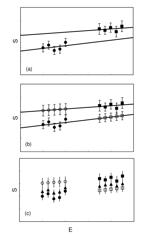
FIG. 1.: Illustration of case 2 (see text). Full circles and squares represent the original experimental data (units are arbitrary); open symbols are extrapolated values, and triangles represent the “effective” cross sections (40).

IV Calculation of Reaction rates

A Definition

The reaction rate $N_{\rm A}\langle\sigma v\rangle$ is defined as [26]

$$N_{\rm A}\langle\sigma v\rangle = N_{\rm A}\ \frac{(8/\pi)^{1/2}}{\mu^{1/2}(k_{\rm B}T)^{3/2}}\int^{\infty}_{0}\sigma E\exp(-E/k_{\rm B}T)\ dE,$$ (42)

where $N_{\rm A}$ is the Avogadro number, $\mu$ the reduced mass of the system, $k_{\rm B}$ the Boltzmann constant, $T$ the temperature, $\sigma$ the cross section, $v$ the relative velocity, and $E$ the energy in the centre-of-mass system. When $N_{\rm A}\langle\sigma v\rangle$ is expressed in cm³ mol^-1 s^-1, the energies $E$ and $k_{\rm B}T$ in MeV, and the cross section $\sigma$ in barn, Eq. (42) leads to

$$N_{\rm A}\langle\sigma v\rangle = 3.7313\times 10^{10}\ \mu_{0}^{-1/2}\,T_{9}^{-3/2}\int^{\infty}_{0}\sigma\,E\,\exp(-11.604E/T_{9})\,dE,$$ (43)

where $\mu_{0}$ is the reduced mass in amu, and $T_{9}$ is the temperature in units of $10^{9}$ K. The calculation of the rates is performed here between $T_{9}=0.001$ and 10, and is compared with previous compilations [5, 6].

Let us first discuss charged-particle reactions. Except near narrow resonances, the $S$-factor is a smooth function of energy, which is convenient for extrapolating measured cross sections down to astrophysical energies. When $S(E)$ is assumed to be a constant, the integrand in Eq. (42) is peaked at the “most effective energy” (the Gamow energy [26]),

$$E_{0}=\left(\frac{\mu}{2}\right)^{1/3}\left(\frac{\pi e^{2}Z_{1}Z_{2}k_{\rm B}T}{\hbar}\right)^{2/3}=0.1220\ (Z_{1}^{2}Z_{2}^{2}\mu_{0})^{1/3}\,T_{9}^{2/3}\ {\rm MeV}$$ (44)

and can be approximated by a Gaussian function centered at $E_{0}$, with full width at $1/e$ of the maximum given by

$$\Delta E_{0}=4\,(E_{0}\ k_{\rm B}T/3)^{1/2}=0.2368\,(Z_{1}^{2}Z_{2}^{2}\mu_{0})^{1/6}\,T_{9}^{5/6}\ {\rm MeV}.$$ (45)

With these approximations, the integral in Eq. (42) can be calculated analytically [26]. However, in the present compilation we do not rely on such approximations and perform numerically the integration of Eq. (42). A good accuracy is reached by limiting the numerical integration for a given temperature to the energy domain ($E_{0}-n\Delta E_{0},E_{0}+n\Delta E_{0}$), with typically $n=2$ or 3. The accuracy is such that at least 4 digits on the rate are significant. For neutron-induced reactions, Eq. (42) is integrated numerically from $E=0$ to $E=nk_{B}T$, where $n$ is typically 10.

Table V presents the rate in a numerical format. To interpolate we recommend to following procedure. As is it well known [5], the non-resonant reaction rate can be parametrized as

$$N_{\rm A}\langle\sigma v\rangle=\exp(-C_{0}/T^{1/3})f_{0}(T)/T^{2/3},$$ (46)

where $C_{0}$ only depends on masses and charges of the system, and is defined by

$$C_{0}=3\left[\pi\frac{e^{2}}{\hbar c}Z_{1}Z_{2}(\frac{\mu c^{2}}{2k_{B}})^{1/2}\right]^{\frac{2}{3}},$$ (47)

and where $f_{0}(T)$ is a smooth function of $T$. Interpolating $f_{0}(T)$ or $\log\,f_{0}(T)$ with a spline method provides the rates with a good accuracy (typically better than 0.1%).

B Screening effects

In stellar plasmas, atoms are usually completely ionized, and nuclear reactions involve bare nuclei. The situation is different in laboratories since target nuclei are partially- or un-ionized. Consequently the role of the electron cloud cannot be neglected at low energies. Let us notice that screening effects, with a different origin, may also occur in stars, but this issue is far beyond our topic.

The screening effect is usually evaluated through the screening potential $U_{e}$. The screening factor [27] is defined as

$$f(E)=\frac{\sigma_{exp}(E)}{\sigma_{th}(E)}=\frac{\sigma_{th}(E+U_{e})}{\sigma_{th}(E)}\approx\exp(\pi\eta\frac{U_{e}}{E}),$$ (48)

where $\sigma_{exp}(E)$ is the experimental cross section, affected by screening effects, and ${\sigma}_{th}(E)$ the theoretical cross section involving bare nuclei. Here the $R$-matrix fit has been applied at energies unaffected by screening effects, and a screening potential has been deduced. For an extended $R$-matrix analysis of electron-screening effects, see for example ref. [28].

C Physical constants

In the analysis of the cross sections and in the calculation of the reaction rates, we have used the atomic masses as recommended by Audi et al. [29]. The following values of the physical constants are used:

$$c = 299792458\ {\rm m\,s}^{-1}$$ (49)

$$1\ amu = 931.494\ {\rm MeV}/c^{2}$$ (50)

$$1\ {\rm eV} = 1.60218\times 10^{-19}\ {\rm J}$$ (51)

$$k_{\rm B}T = 0.08617\,T_{9}=T_{9}/11.605\ {\rm MeV}$$ (52)

$$N_{\rm A} = 6.0221\times 10^{23}\ {\rm mol}^{-1}$$ (53)

$$\alpha = e^{2}/\hbar c=1/137.036$$ (54)

$$\hbar c = 197.327\ {\rm MeV.fm}$$ (55)

V Cross sections and reaction rates

²H(p,$\gamma$)³He
The data of ref. [30] are superseded by ref. [31] and are therefore not included. Very recent data [17] allow a more precise extrapolation down to low energies. Below 0.01 MeV, the $S$ factor is nearly constant which is typical of $s$-wave capture, proceeding by an M1 transition. At zero energy, our partial $S$ factors $0.089\pm 0.004$ eV.b (E1) and $0.134\pm 0.006$ eV.b (M1) are consistent with the values recommended by Schmid et al. [31] ($0.073$ eV.b and $0.109$ eV.b, respectively) from polarized-data measurements. Our results are slightly higher than NACRE, which uses a polynomial fit for the $S$ factor.

²H(d,n)³He and ²H(d,p)³H
Two non-resonant partial waves are included in the fit. The fits have been performed individually (data of refs. [32, 33, 34]), with each of them being complemented by the high-energy data of ref. [35]. The recommended $S$ factors have been deduced as explained in Sec. III. The individual fits are given in figs I.b and I.c as dotted lines. As shown in Ref.[23] it is not possible to optimize the fits of both reactions with the same parameter set. Consequently the $R$-matrix parameters are somewhat different. The reaction rates are close to the results of NACRE, but the uncertainties have been reduced.

³H(d,n)⁴He
In addition to the well known low-energy $3/2^{+}$ resonance ($\ell_{i}=0$), non-resonant contributions from the $1/2^{+}\ (\ell_{i}=0)$ and $1/2^{-},3/2^{-}\ (\ell_{i}=1)$ partial waves have been included. The present $R$-matrix fit is very close to the fit of Hale [36], and yields a fairly low uncertainty on the reaction rate. We find a reaction rate similar to NACRE, except at high temperatures, where NACRE uses very conservative lower and upper bounds.

³H($\alpha,\gamma)^{7}$Li
The data of refs. [37, 38] have not been included as they are obviously inconsistent with the other data sets. The $s-$ and $d$-wave contributions are taken into account. To reduce the number of free parameters, we have adopted, for ³H($\alpha,\gamma)^{7}$Li and ³He($\alpha,\gamma)^{7}$Be, the same ANC values for the ground and first excited states. This seems reasonable as both states arise from the same isospin doublet. The statistical method adopted here provides error bars significantly lower than in NACRE, where a very conservative technique was used. At high energies, the reaction rates are slightly different; in spite of the lack of data above 1.2 MeV, the $R$-matrix approach is expected to be more reliable than the polynomial extrapolation used in NACRE.

³He(n,p)³H
In the low-energy region, the main partial waves correspond to $\ell=0$ and 1. According to the ⁴He energy spectrum, the $0^{+}_{2}\ (E_{x}=20.21$ MeV), $0^{-}\ (E_{x}=21.01$ MeV) and $2^{-}\ (E_{x}=21.84$ and 23.33 MeV) states are expected to determine the cross section. They correspond to ($\ell I)=(0,0),(1,1)$ and (1,1), respectively. The role of the two broad $2^{-}$ resonances has been simulated by a single pole in the $R$-matrix expansion. An $\ell=0$ non-resonant partial wave, corresponding to $J=1^{+}$ has been also taken into account. The data of Brune et al. [16] suggest a new $0^{-}$ resonance at 0.43 MeV which indeed must be included to optimize the fit. More detail can be found in Ref. [39].

³He(d,p)⁴He
The dominance of the $\ell=0$ contribution at low energy is confirmed by the isotropic angular distributions [40], but a ${\ell_{i}=1}$ component has been included to improve the quality of the fit. The Coulomb dependence involved in the $R$ matrix approach leads to differences up to 10% with the polynomial expansion used by Krauss et al. [40]. This explains the differences with previous compilations [5, 6]. Our rate is in good agreement with the fit of Hale [36].
The low-energy data of Refs. [41] and [42] are affected by electron-screening effects. The former are obtained through the d(³He,p)⁴He reaction, and are complemented by a subset of the latter data [42]. The screening potentials are found as $U_{e}=146\pm 5$ eV for the d(³He,p)⁴He reaction, and $U_{e}=201\pm 10$ eV for the ³He(d,p)⁴He reaction. These values are somewhat different from those derived in ref.[42] ($109\pm 9$ eV and $219\pm 7$ eV) where a polynomial approximation is used to determine the bare-nucleus cross sections. According to ref. [42], we do not include the data of refs. [43, 44] as their analysis was biased by stopping-power problems.

³He($\alpha,\gamma)^{7}$Be
A purely external capture has been assumed, with $\ell_{i}=0$ and $\ell_{f}=2$ contributions. The data of ref. [45] are clearly affected by normalization problems, and have not been taken into account. According to Ref. [46], the data of Kräwinkel et al. [47] have been renormalized by 1.4. For this reaction, most data sets allow an extrapolation down to zero energy. Accordingly, an $S(0)$ value, with the associated uncertainty, has been determined for each reaction, and an averaged $S(0)$ has been obtained. Since the capture cross section is assumed to be external, the $S$ factor only depends on the normalization factor. The normalization has been deduced from the adopted $S(0)$. The present $S(0)$ value ($S(0)=0.51\pm 0.04$ keV.b) overlaps with the value recommended by Adelberger et al. [48] ($S(0)=0.53\pm 0.05$ keV.b) and by NACRE [6] ($S(0)=0.54\pm 0.09$ keV.b).

⁷Li(p,$\alpha)\alpha$
The $S$ factor is mainly determined by $\ell_{i}=1,J=0^{+},2^{+}$ contributions. Owing to parity conservation and to the symmetry of the final state, $\ell=0$ partial waves in the entrance channel are forbidden. The ⁸Be spectrum presents two $2^{+}$ states below the ⁷Li+p threshold. These states have been accounted for by a single state at $E=-0.48$ MeV. For the $2^{+}$ resonance at $E=2.60$ MeV, we neglect the interference with the subthreshold state; the energy and widths have been taken from literature, without any fitting procedure.
At very low energies, data affected by electron screening ($E<40$ keV) have not been considered in the fitting procedure. An analysis of the screening potential provides $U_{e}=100\pm 25$ eV. This value is much lower than the value deduced by Engstler et al. ($U_{e}=300\pm 280$ eV for an atomic target, $U_{e}=300\pm 160$ eV for a molecular target) who use a third-order polynomial to determine the bare-nucleus cross section. This procedure is quite questionable here since the low-energy $S$-factor depends on a subthreshold state whose effect is negligible beyond 100 keV. A recent experiment by Lattuada et al. [49] uses the Trojan Horse Method which does not depend on electron screening, and provides $S(0)=55\pm 3$ keV.b by a polynomial extrapolation. The present analysis provides a significantly higher $S$ factor at low energy ($S(0)=67\pm 4$ keV.b). This discrepancy is confirmed by a recent $R$-matrix analysis of Barker [50, 28] who finds values similar to ours.

⁷Be(n,p)⁷Li
The $2^{-}$ state located very near threshold determines the cross section in a wide energy range. To reproduce the data up to 5 MeV we have included the $3^{+}$ resonances at $E=0.34$ MeV and $E=2.60$ MeV. We neglect interference effects. Our reaction rate is consistent with the SKM compilation up to $T_{9}\approx 4$, but provides larger values above this temperature. More detail can be found in Ref. [39].

VI References

Explanation of tables

  TABLE I

$R$-matrix parameters (observed values).
The observed values are given. The channel radius $a$ is taken as $a=5$ fm, except for the ³H($\alpha,\gamma)^{7}$Li and ³He($\alpha,\gamma)^{7}$Be reactions, where $a=3$ fm. Non-fitted parameters are shown in italics.
Capture reactions:
$\ell_{i},J_{i}$: orbital momentum and total spin of the initial state.
$\ell_{f},J_{f},E_{f},C_{f}$: orbital momentum, total spin, energy and ANC of the final state ($E_{f}$ is taken from literature).
$E_{1}^{r},\Gamma_{i},\Gamma_{f}$: $R$-matrix parameters (see Sec.II).

Transfer reactions:
$\ell_{i},J_{i}$: orbital momentum and total spin of the initial state.
$\ell_{f}$: orbital momentum of the final state.
$E_{1}^{r},\Gamma_{i},\Gamma_{f}$: $R$-matrix parameters for resonant partial waves.
$R_{i},R_{f}$: $R$-matrix parameters for non-resonant partial waves.

  TABLE II

Covariance matrices.
The covariance matrices $C$ are calculated from Eq.(37). Units are chosen as in Table I.

  TABLE III

Zero-energy $S$ factors (or $\left(\sigma(E)\sqrt{(}E)\right)_{0}$ for neutron-capture reactions).

  TABLE IV.a-b

$S$-factors.
Energies are chosen from zero to the experimental upper limits, with a step which provides an accurate interpolation.

  TABLE V

Analytical fits of the reactions rates.
$T_{9}^{max}$: maximum value of $T_{9}$ for which the fit reproduces the numerical values of Tables VI with an accuracy better than 5%.
The parametrization is as follows:

$$N_{\rm A}\langle\sigma v\rangle = d_{0}\ \frac{\exp(-C_{0}/T_{9}^{1/3})}{T_{9}^{2/3}}\times(1+\sum_{i=1}^{3}d_{i}T_{9}^{i}){\rm\ for\ charged\ particles}$$ (56)

$$N_{\rm A}\langle\sigma v\rangle = d_{0}\ (1+\sum_{i=1}^{3}d_{i}T_{9}^{i}){\rm\ for\ neutrons},$$ (57)

with units:
$T_{9}:10^{9}\,K$,
$C_{0}:K^{1/3}$,
$N_{\rm A}\langle\sigma v\rangle,d_{0}:$ cm³ mol^-1 s^-1,

  TABLE VI.a-j

Reaction rates (in cm³ mol^-1 s^-1).
$E_{0},\Delta E_{0}$ (in MeV): see Eqs. (44) and (45)
NACRE: ratio of the adopted rate with respect to the NACRE rate [6]
SKM: ratio of the adopted rate with respect to the SKM rate [9]
Lower and upper values correspond the one-sigma uncertainties.

Explanation of graphs

  Figures I.a-j

$S$-factors
The figures represent the $S$ factors for charged particles, and $\sigma(E)\sqrt{E}$ for neutron induced reactions (full curves), versus c.m. energy. If not specified, the dotted curves represent the lower and upper limits.

  Figures II.a-b

Reaction rates
Reaction rates normalized to the NACRE adopted rates, or to the SKM rates for the ³He(d,p)⁴He, ³He(n,p)³H, and ⁷Be(n,p)⁷Li reactions not available in NACRE. Solid curves correspond to the present reaction rates, dashed curves to the SKM rates and dotted curves to the NACRE upper and lower limits.

TABLE I.: $R$-matrix parameters (observed values). Energies and widths are expressed in MeV and ANC in fm^-1/2. $R$ matrices are dimensionless. The reduced $\chi^{2}$ values are given in brackets.

Capture reactions	$\ell_{i}$	$J_{i}$	$\ell_{f}$	$J_{f}$	$E_{f}$	$C_{f}$	$E^{r}_{1}$	$\Gamma_{i}$	$\Gamma_{f}$
2H(p,$\gamma$)3He (0.55)	1	$3/2^{-}$	0	$1/2^{+}$	-5.49	-1.78	10	23.4	$4.20\times 10^{-4}$
	0	$1/2^{+}$	0	$1/2^{+}$	-5.49	-1.78	10	23.4	$7.28\times 10^{-5}$
3H($\alpha,\gamma)^{7}$Li (0.16)	0	$1/2^{+}$	1	$3/2^{-}$	-2.47	-3.49	10	4.87	$1.71\times 10^{-2}$
	2a)	$5/2^{+}$	1	$3/2^{-}$	-2.47	-3.49
	0	$1/2^{+}$	1	$1/2^{-}$	-1.99	-3.49	10	4.87	$3.70\times 10^{-3}$
	2a)	$3/2^{+}$	1	$1/2^{-}$	-1.99	-3.49
$\mbox{${}^{3}$He($\alpha,\gamma)^{7}$Be}^{a)}$ (1.46)	0	$1/2^{+}$	1	$3/2^{-}$	-1.54	3.79
	2	$5/2^{+}$	1	$3/2^{-}$	-1.54	3.79
	0	$1/2^{+}$	1	$1/2^{-}$	-1.19	3.79
	2	$3/2^{+}$	1	$1/2^{-}$	-1.19	3.79
Transfer reactions	$\ell_{i}$	$J_{i}$	$\ell_{f}$	$E^{r}_{1}$	$\Gamma_{i}$ (or $R_{i}$)	$\Gamma_{f}$ (or $R_{f}$)
2H(d,n)3He (1.20)	0	$2^{+}$	2		1.67	0.0129
	1	$0^{-},1^{-},2^{-}$	1		0.0895	0.550
2H(d,p)3H (1.17)	0	$2^{+}$	2		0.621	0.0174
	1	$0^{-},1^{-},2^{-}$	1		0.0853	0.275
3H(d,n)4He (1.20)	0	$3/2^{+}$	2	0.0938	0.177	0.0940
	1	$1/2^{-},3/2^{-}$	1		0.429	1.85
3He(d,p)4He (0.89)	0	$3/2^{+}$	2	0.248	0.0405	0.215
	1	$1/2^{-},3/2^{-}$	1		1.20	1.41
3He(n,p)3H (0.36)	0	$0^{+}$	0	-0.221	2.291b)	1.164
	0	$1^{+}$	0		0.158	0.193
	1	$2^{-}$	1	2.61	4.529	4.279
	1	$0^{-}$	1	0.43	0.479	0.0480
7Li(p,$\alpha)\alpha$ (0.46)	1	$2^{+}$	2	-0.48	0.0959b)	0.0954
	1	$2^{+}$	2	2.6	0.085	0.830
	1	$0^{+}$	0		0.081	0.138
7Be(n,p)7Li (0.90)	0	$2^{-}$	0	0.00267	0.225	1.41
	1	$3^{+}$	1	0.330	0.0767	0.088
	1	$3^{+}$	1	2.66	0.490	0.610
	1	$2^{+}$	1		3.01	2.90

^a) External capture only.
^b) Reduced width $\gamma_{i}^{2}$.

TABLE II.: Covariance matrices.

Capture reactions
2H(p,$\gamma$)3He	$\Gamma_{i}(3/2^{-})$	$\Gamma_{f}(3/2^{-})$	$C_{f}$	$\Gamma_{f}(1/2^{+})$
$\Gamma_{i}(3/2^{-})$	5.54E+00	1.38E-04	3.06E-01	-7.12E-06
$\Gamma_{f}(3/2^{-})$	1.38E-04	4.39E-09	9.02E-06	-1.34E-10
$C_{f}$	3.06E-01	9.02E-06	1.98E-02	-2.66E-07
$\Gamma_{f}(1/2^{+})$	-7.12E-06	-1.34E-10	-2.66E-07	1.76E-11
3H($\alpha,\gamma)^{7}$Li	$\Gamma_{i}(1/2^{+})$	$\Gamma_{f}(1/2^{+}\rightarrow 3/2^{-})$	$C_{f}$	$\Gamma_{f}(1/2^{+}\rightarrow 1/2^{-})$
$\Gamma_{i}(1/2^{+})$	1.81E+03	-1.14E+00	-9.18E+01	-2.38E+00
$\Gamma_{f}(1/2^{+}\rightarrow 3/2^{-})$	-1.14E+00	1.07E-03	4.70E-02	1.44E-03
$C_{f}$	-9.18E+01	4.70E-02	5.01E+00	1.23E-01
$\Gamma_{f}(1/2^{+}\rightarrow 1/2^{-})$	-2.38E+00	1.44E-03	1.23E-01	3.15E-03
3He($\alpha,\gamma)^{7}$Be	$C_{f}$
$C_{f}$	2.25E-02
Transfer reactions
2H(d,n)3He	$R_{i}(2^{+})$	$R_{f}(2^{+})$	$R_{i}(0^{-},1^{-},2^{-})$	$R_{f}(0^{-},1^{-},2^{-})$
$R_{i}(2^{+})$	3.90E-02	-8.20E-05	1.68E-04	-4.12E-03
$R_{f}(2^{+})$	-8.20E-05	2.10E-07	-3.51E-07	-8.26E-07
$R_{i}(0^{-},1^{-},2^{-})$	1.68E-04	-3.51E-07	1.61E-06	-3.43E-05
$R_{f}(0^{-},1^{-},2^{-})$	-4.12E-03	-8.26E-07	-3.43E-05	3.71E-03
2H(d,p)3H	$R_{i}(2^{+})$	$R_{f}(2^{+})$	$R_{i}(0^{-},1^{-},2^{-})$	$R_{f}(0^{-},1^{-},2^{-})$
$R_{i}(2^{+})$	7.10E-03	-1.16E-04	9.49E-04	-4.92E-03
$R_{f}(2^{+})$	-1.16E-04	1.92E-06	-1.50E-05	7.72E-05
$R_{i}(0^{-},1^{-},2^{-})$	9.49E-04	-1.50E-05	1.79E-04	-9.42E-04
$R_{f}(0^{-},1^{-},2^{-})$	-4.92E-03	7.72E-05	-9.42E-04	5.00E-03
3H(d,n)4He	$E_{1}^{r}(3/2^{+})$	$\Gamma_{i}(3/2^{+})$	$\Gamma_{f}(3/2^{+})$	$R_{i}(1/2^{-},3/2^{-})$	$R_{f}(1/2^{-},3/2^{-})$
$E_{1}^{r}(3/2^{+})$	1.01E-06	9.06E-06	2.39E-06	6.26E-04	2.81E-03
$\Gamma_{i}(3/2^{+})$	9.06E-06	8.27E-05	2.11E-05	9.26E-03	4.17E-02
$\Gamma_{f}(3/2^{+})$	2.39E-06	2.11E-05	6.00E-06	-3.63E-04	-1.66E-03
$R_{i}(1/2^{-},3/2^{-})$	6.26E-04	9.26E-03	-3.63E-04	3.02E+01	1.36E+02
$R_{f}(1/2^{-},3/2^{-})$	2.81E-03	4.17E-02	-1.66E-03	1.36E+02	6.15E+02
3He(d,p)4He	$E_{1}^{r}(3/2^{+})$	$\Gamma_{i}(3/2^{+})$	$\Gamma_{f}(3/2^{+})$	$R_{i}(1/2^{-},3/2^{-})$	$R_{f}(1/2^{-},3/2^{-})$
$E_{1}^{r}(3/2^{+})$	6.73E-06	6.72E-06	1.08E-05	-2.68E-02	-3.58E-02
$\Gamma_{i}(3/2^{+})$	6.72E-06	7.92E-06	1.22E-05	-3.54E-02	-4.75E-02
$\Gamma_{f}(3/2^{+})$	1.08E-05	1.22E-05	2.87E-05	-5.30E-02	-7.10E-02
$R_{i}(1/2^{-},3/2^{-})$	-2.68E-02	-3.54E-02	-5.30E-02	1.83E+02	2.46E+02
$R_{f}(1/2^{-},3/2^{-})$	-3.58E-02	-4.75E-02	-7.10E-02	2.46E+02	3.31E+02
3He(n,p)3H	$\Gamma_{i}(0^{+})$	$R_{i}(1^{+})$	$R_{f}(1^{+})$	$\Gamma_{i}(2^{-})$	$\Gamma_{f}(2^{-})$	$\Gamma_{i}(0^{-})$	$\Gamma_{f}(0^{-})$
$\Gamma_{i}(0^{+})$	1.14E-01	2.29E+00	-2.46E+00	1.33E-01	-1.42E-01	-6.73E-03	-4.41E-04
$R_{i}(1^{+})$	2.29E+00	5.43E+01	-5.84E+01	3.90E+00	-3.87E+00	-1.16E-01	-1.95E-03
$R_{f}(1^{+})$	-2.46E+00	-5.84E+01	6.28E+01	-4.20E+00	4.17E+00	1.25E-01	2.02E-03
$\Gamma_{i}(2^{-})$	1.33E-01	3.90E+00	-4.20E+00	1.02E+00	-1.14E+00	-7.86E-03	3.71E-03
$\Gamma_{f}(2^{-})$	-1.42E-01	-3.87E+00	4.17E+00	-1.14E+00	1.32E+00	1.07E-02	-4.60E-03
$\Gamma_{i}(0^{-})$	-6.73E-03	-1.16E-01	1.25E-01	-7.86E-03	1.07E-02	2.75E-03	1.38E-04
$\Gamma_{f}(0^{-})$	-4.41E-04	-1.95E-03	2.02E-03	3.71E-03	-4.61E-03	1.38E-04	4.58E-05
7Li(p,$\alpha)\alpha$	$\Gamma_{i}(2^{+}_{1})$	$\Gamma_{f}(2^{+}_{1})$	$R_{i}(0^{+})$	$R_{f}(0^{+})$
$\Gamma_{i}(2^{+}_{1})$	1.67E+00	-1.33E+00	-5.65E-02	6.50E-01
$\Gamma_{f}(2^{+}_{1})$	-1.33E+00	1.06E+00	4.51E-02	-5.18E-01
$R_{i}(0^{+})$	-5.65E-02	4.51E-02	2.58E-03	-2.77E-02
$R_{f}(0^{+})$	6.50E-01	-5.18E-01	-2.77E-02	3.03E-01
7Be(n,p)7Li	$E^{r}_{1}(2^{-})$	$\Gamma_{i}(3^{+}_{1})$	$\Gamma_{f}(3^{+}_{1})$	$R_{i}(2^{+})$	$R_{f}(2^{+})$
$E^{r}_{1}(2^{-})$	1.09E-10	-9.23E-10	1.69E-10	-1.02E-07	5.96E-08
$\Gamma_{i}(3^{+}_{1})$	-9.23E-10	1.59E-04	-1.28E-04	-1.33E-03	-1.90E-02
$\Gamma_{f}(3^{+}_{1})$	1.69E-10	-1.28E-04	1.89E-04	-5.41E-03	-7.26E-03
$R_{i}(2^{+})$	-1.02E-07	-1.33E-03	-5.41E-03	1.92E+00	7.79E-01
$R_{f}(2^{+})$	5.96E-08	-1.90E-02	-7.26E-03	7.79E-01	1.08E+01

TABLE III.: $S$ factors at zero energy (or $\left(\sigma(E)\sqrt{(}E)\right)_{0}$ for neutron-capture reactions).

Reaction	$S(0)$ or $\left(\sigma(E)\sqrt{(}E)\right)_{0}$
2H(p,$\gamma$)3He	$0.223\pm 0.010$ eV-b (E1:$0.089\pm 0.004$, M1:$0.134\pm 0.006$)
2H(d,n)3He	$52.4\pm 3.5$ keV-b
2H(d,p)3H	$57.1\pm 0.8$ keV-b
3H(d,n)4He	$11.7\pm 0.2$ MeV-b
3H($\alpha,\gamma)^{7}$Li	$0.095\pm 0.005$ keV-b
3He(n,p)3H	$0.70\pm 0.01$ MeV1/2-b
3He(d,p)4He	$5.9\pm 0.3$ MeV-b
3He($\alpha,\gamma)^{7}$Be	$0.51\pm 0.04$ keV-b
7Li(p,$\alpha)\alpha$	$67\pm 4$ keV-b
7Be(n,p)7Li	$5.75\pm 0.04$ MeV1/2-b

TABLE IV.a.: $S$-factors

$E$	2H(p,$\gamma$)3He	$E$	2H(d,n)3He	$E$	2H(d,p)3H	$E$	3H(d,n)4He	$E$	3H($\alpha,\gamma)^{7}$Li
(MeV)	(eV-b)	(MeV)	(MeV-b)	(MeV)	(MeV-b)	(MeV)	(MeV-b)	(MeV)	(keV-b)
0.001	2.29E-01	0.001	5.29E-02	0.001	5.73E-02	0.001	1.19E01	0.001	9.47E-02
0.002	2.35E-01	0.002	5.33E-02	0.002	5.75E-02	0.002	1.21E01	0.002	9.46E-02
0.005	2.50E-01	0.005	5.43E-02	0.005	5.79E-02	0.005	1.26E01	0.005	9.43E-02
0.010	2.76E-01	0.010	5.60E-02	0.010	5.86E-02	0.010	1.38E01	0.010	9.38E-02
0.020	3.29E-01	0.020	5.95E-02	0.020	6.01E-02	0.020	1.71E01	0.020	9.28E-02
0.050	4.98E-01	0.050	7.05E-02	0.050	6.48E-02	0.050	2.69E01	0.050	8.98E-02
0.100	8.10E-01	0.100	8.79E-02	0.100	7.39E-02	0.100	9.93E00	0.100	8.45E-02
0.200	1.52E00	0.200	1.17E-01	0.200	9.43E-02	0.200	2.27E00	0.200	7.48E-02
0.350	2.76E00	0.350	1.54E-01	0.300	1.15E-01	0.250	1.55E00	0.300	6.77E-02
0.500	4.16E00	0.500	1.87E-01	0.400	1.35E-01	0.300	1.17E00	0.400	6.32E-02
0.650	5.69E00	0.650	2.17E-01	0.500	1.54E-01	0.350	9.49E-01	0.500	6.05E-02
0.800	7.32E00	0.800	2.45E-01	0.600	1.73E-01	0.400	8.09E-01	0.600	5.92E-02
0.950	9.06E00	0.950	2.71E-01	0.700	1.90E-01	0.450	7.12E-01	0.700	5.90E-02
1.100	1.09E01	1.100	2.95E-01	0.800	2.07E-01	0.500	6.43E-01	0.800	5.96E-02
1.250	1.28E01	1.250	3.18E-01	0.900	2.23E-01	0.550	5.91E-01	0.900	6.08E-02
1.400	1.47E01	1.400	3.39E-01	1.000	2.39E-01	0.600	5.52E-01	1.000	6.27E-02
1.550	1.67E01	1.550	3.58E-01	1.100	2.53E-01	0.650	5.22E-01	1.100	6.50E-02
1.700	1.88E01	1.700	3.76E-01	1.200	2.67E-01	0.700	4.98E-01	1.200	6.78E-02
1.850	2.09E01	1.850	3.93E-01	1.300	2.81E-01	0.750	4.78E-01	1.300	7.09E-02
2.000	2.30E01	2.000	4.09E-01	1.400	2.94E-01	0.800	4.63E-01	1.400	7.44E-02
2.150	2.52E01	2.150	4.24E-01	1.500	3.07E-01	0.850	4.49E-01	1.500	7.83E-02
2.300	2.74E01	2.300	4.38E-01	1.600	3.19E-01	0.900	4.39E-01	1.600	8.25E-02
2.450	2.96E01	2.450	4.51E-01	1.700	3.31E-01	0.950	4.29E-01	1.700	8.71E-02
2.600	3.18E01	2.600	4.64E-01	1.800	3.42E-01	1.000	4.22E-01	1.800	9.19E-02
2.750	3.40E01	2.750	4.76E-01	1.900	3.54E-01	1.050	4.15E-01	1.900	9.71E-02
2.900	3.62E01	2.900	4.87E-01	2.000	3.64E-01	1.100	4.10E-01	2.000	1.03E-01
3.050	3.83E01	3.050	4.97E-01	2.100	3.75E-01	1.150	4.05E-01	2.100	1.09E-01
3.200	4.05E01	3.200	5.07E-01	2.200	3.85E-01	1.200	4.01E-01	2.200	1.15E-01
3.350	4.26E01	3.350	5.17E-01	2.300	3.95E-01	1.250	3.97E-01	2.300	1.22E-01
3.500	4.47E01	3.500	5.26E-01	2.400	4.05E-01	1.300	3.94E-01	2.400	1.29E-01
3.650	4.68E01	3.650	5.34E-01	2.500	4.14E-01	1.350	3.92E-01	2.500	1.36E-01
3.800	4.88E01	3.800	5.42E-01	2.600	4.23E-01	1.400	3.90E-01	2.600	1.44E-01
3.950	5.08E01	3.950	5.50E-01	2.700	4.32E-01	1.450	3.88E-01	2.700	1.53E-01
4.100	5.28E01	4.100	5.57E-01	2.800	4.41E-01	1.500	3.86E-01	2.800	1.62E-01
4.250	5.47E01	4.250	5.64E-01	2.900	4.49E-01	1.550	3.84E-01	2.900	1.71E-01
4.400	5.65E01	4.400	5.71E-01	3.000	4.58E-01	1.600	3.83E-01	3.000	1.82E-01
4.550	5.84E01	4.550	5.77E-01	3.100	4.66E-01	1.650	3.82E-01	3.100	1.93E-01
4.700	6.01E01	4.700	5.83E-01	3.200	4.74E-01	1.700	3.81E-01	3.200	2.05E-01
4.850	6.18E01	4.850	5.89E-01	3.300	4.81E-01	1.750	3.80E-01	3.300	2.17E-01
5.000	6.35E01	5.000	5.94E-01	3.400	4.89E-01	1.800	3.79E-01	3.400	2.29E-01
5.150	6.51E01	5.150	6.00E-01	3.500	4.96E-01	1.850	3.79E-01	3.500	2.42E-01
5.300	6.66E01	5.300	6.05E-01	3.600	5.04E-01	1.900	3.78E-01	3.600	2.56E-01
5.450	6.81E01	5.450	6.09E-01	3.700	5.11E-01	1.950	3.78E-01	3.700	2.72E-01
5.600	6.96E01	5.600	6.14E-01	3.800	5.17E-01	2.000	3.77E-01	3.800	2.92E-01
5.750	7.10E01	5.750	6.18E-01	3.900	5.24E-01	2.050	3.77E-01	3.900	3.16E-01
5.900	7.23E01	5.900	6.22E-01	4.000	5.31E-01	2.100	3.77E-01	4.000	3.40E-01
6.050	7.36E01	6.050	6.26E-01	4.100	5.37E-01	2.150	3.77E-01	4.100	3.62E-01
6.200	7.49E01	6.200	6.30E-01	4.200	5.43E-01	2.200	3.76E-01	4.200	3.78E-01
6.350	7.61E01	6.350	6.34E-01	4.300	5.50E-01	2.250	3.76E-01	4.300	3.85E-01
6.500	7.73E01	6.500	6.38E-01	4.400	5.56E-01	2.300	3.76E-01	4.400	3.92E-01
6.650	7.84E01	6.650	6.41E-01	4.500	5.62E-01	2.350	3.76E-01	4.500	4.12E-01
6.800	7.95E01	6.800	6.44E-01	4.600	5.68E-01	2.400	3.76E-01	4.600	4.58E-01

TABLE IV.b.: $S$-factors

$E$	3He(n,p)3H	$E$	3He(d,p)4He	$E$	3He($\alpha,\gamma)^{7}$Be	$E$	7Li(p,$\alpha)\alpha$	$E$	7Be(n,p)7Li
(MeV)	(b-MeV1/2)	(MeV)	(MeV-b)	(MeV)	(keV-b)	(MeV)	(MeV-b)	(MeV)	(b-MeV1/2)
0.001	6.86E-01	0.001	5.92E00	0.001	5.10E-01	0.001	6.66E-02	0.001	4.77E00
0.002	6.73E-01	0.002	5.95E00	0.002	5.10E-01	0.002	6.66E-02	0.002	4.44E00
0.005	6.46E-01	0.005	6.03E00	0.005	5.09E-01	0.005	6.69E-02	0.005	3.87E00
0.010	6.18E-01	0.010	6.19E00	0.010	5.07E-01	0.010	6.79E-02	0.010	3.35E00
0.020	5.80E-01	0.020	6.51E00	0.020	5.04E-01	0.020	6.91E-02	0.020	2.79E00
0.050	5.16E-01	0.050	7.67E00	0.050	4.94E-01	0.050	7.20E-02	0.050	2.03E00
0.100	4.67E-01	0.100	1.03E01	0.100	4.79E-01	0.100	7.61E-02	0.100	1.54E00
0.200	4.62E-01	0.200	1.70E01	0.200	4.48E-01	0.200	8.21E-02	0.200	1.30E00
0.400	5.76E-01	0.300	1.19E01	0.250	4.33E-01	0.400	9.13E-02	0.250	1.49E00
0.600	6.31E-01	0.400	5.65E00	0.300	4.18E-01	0.600	1.01E-01	0.300	1.91E00
0.800	7.37E-01	0.500	3.36E00	0.350	4.04E-01	0.800	1.11E-01	0.350	1.89E00
1.000	8.42E-01	0.600	2.47E00	0.400	3.90E-01	1.000	1.33E-01	0.400	1.47E00
1.200	9.18E-01	0.700	2.07E00	0.450	3.77E-01	1.200	1.45E-01	0.450	1.19E00
1.400	9.59E-01	0.800	1.87E00	0.500	3.64E-01	1.400	1.72E-01	0.500	1.03E00
1.600	9.71E-01	0.900	1.76E00	0.550	3.52E-01	1.600	2.13E-01	0.550	9.11E-01
1.800	9.63E-01	1.000	1.68E00	0.600	3.42E-01	1.800	2.79E-01	0.600	8.25E-01
2.000	9.45E-01	1.100	1.63E00	0.650	3.30E-01	2.000	3.89E-01	0.650	7.63E-01
2.200	9.19E-01	1.200	1.59E00	0.700	3.23E-01	2.200	5.71E-01	0.700	7.21E-01
2.400	8.90E-01	1.300	1.57E00	0.750	3.14E-01	2.400	8.20E-01	0.750	6.96E-01
2.600	8.61E-01	1.400	1.55E00	0.800	3.07E-01	2.600	9.61E-01	0.800	6.84E-01
2.800	8.32E-01	1.500	1.53E00	0.850	3.01E-01	2.800	8.18E-01	0.850	6.82E-01
3.000	8.04E-01	1.600	1.51E00	0.900	2.95E-01	3.000	5.84E-01	0.900	6.84E-01
3.200	7.78E-01	1.700	1.49E00	0.950	2.90E-01	3.200	4.11E-01	0.950	6.89E-01
3.400	7.54E-01	1.800	1.47E00	1.000	2.85E-01	3.400	3.06E-01	1.000	6.91E-01
3.600	7.31E-01	1.900	1.46E00	1.050	2.81E-01	3.600	2.41E-01	1.050	6.90E-01
3.800	7.08E-01	2.000	1.44E00	1.100	2.78E-01	3.800	2.00E-01	1.100	6.86E-01
4.000	6.86E-01	2.100	1.43E00	1.150	2.75E-01	4.000	1.72E-01	1.150	6.80E-01
4.200	6.65E-01	2.200	1.42E00	1.200	2.72E-01	4.200	1.53E-01	1.200	6.71E-01
4.400	6.49E-01	2.300	1.40E00	1.250	2.70E-01	4.400	1.37E-01	1.250	6.62E-01
4.600	6.39E-01	2.400	1.39E00	1.300	2.68E-01	4.600	1.27E-01	1.300	6.52E-01
4.800	6.35E-01	2.500	1.38E00	1.350	2.67E-01	4.800	1.20E-01	1.350	6.43E-01
5.000	6.33E-01	2.600	1.37E00	1.400	2.66E-01	5.000	1.16E-01	1.400	6.35E-01
5.200	6.31E-01	2.700	1.36E00	1.450	2.65E-01	5.200	1.12E-01	1.450	6.28E-01
5.400	6.25E-01	2.800	1.35E00	1.500	2.64E-01	5.400	1.09E-01	1.500	6.23E-01
5.600	6.11E-01	2.900	1.34E00	1.550	2.64E-01	5.600	1.06E-01	1.550	6.20E-01
5.800	5.88E-01	3.000	1.33E00	1.600	2.64E-01	5.800	1.04E-01	1.600	6.19E-01
6.000	5.51E-01	3.100	1.32E00	1.650	2.64E-01	6.000	1.01E-01	1.650	6.20E-01
6.200	5.98E-01	3.200	1.31E00	1.700	2.64E-01	6.200	9.93E-02	1.700	6.21E-01
6.400	5.84E-01	3.300	1.30E00	1.750	2.64E-01	6.400	9.74E-02	1.750	6.25E-01
6.600	5.69E-01	3.400	1.29E00	1.800	2.65E-01	6.600	9.57E-02	1.800	6.29E-01
6.800	5.52E-01	3.500	1.28E00	1.850	2.65E-01	6.800	9.43E-02	1.850	6.34E-01
7.000	5.34E-01	3.600	1.27E00	1.900	2.66E-01	7.000	9.30E-02	1.900	6.41E-01
7.200	5.16E-01	3.700	1.27E00	1.950	2.67E-01	7.200	9.19E-02	1.950	6.49E-01
7.400	4.98E-01	3.800	1.26E00	2.000	2.68E-01	7.400	9.09E-02	2.000	6.58E-01
7.600	4.81E-01	3.900	1.25E00	2.050	2.69E-01	7.600	9.01E-02	2.050	6.70E-01
7.800	4.65E-01	4.000	1.24E00	2.100	2.70E-01	7.800	8.94E-02	2.100	6.83E-01
8.000	4.50E-01	4.100	1.24E00	2.150	2.71E-01	8.000	8.88E-02	2.150	6.99E-01
8.200	4.38E-01	4.200	1.23E00	2.200	2.72E-01	8.200	8.83E-02	2.200	7.17E-01
8.400	4.27E-01	4.300	1.22E00	2.250	2.73E-01	8.400	8.79E-02	2.250	7.37E-01
8.600	4.19E-01	4.400	1.22E00	2.300	2.75E-01	8.600	8.76E-02	2.300	7.58E-01
8.800	4.11E-01	4.500	1.21E00	2.350	2.76E-01	8.800	8.73E-02	2.350	7.79E-01
9.000	4.05E-01	4.600	1.20E00	2.400	2.78E-01	9.000	8.72E-02	2.400	7.99E-01

TABLE  V.: Analytical fits of the adopted reaction rates.

Reaction	$C_{0}$	$d_{0}$	$d_{1}$	$d_{2}$	$d_{3}$	$T_{9}^{max}$
2H(p,$\gamma$)3He	3.7208	2.173E+03	6.899	-4.442	3.134	0.8
2H(d,n)3He	4.2586	4.371E+08	1.737	-0.633	0.109	3
2H(d,p)3H	4.2586	4.682E+08	0.745	-0.065	0.003	3
3H(d,n)4He	4.5244	8.656E+10	14.002	-59.683	64.236	0.5
3H($\alpha,\gamma)^{7}$Li	8.0805	7.717E+05	-0.268	0.068	-0.004	8
3He(n,p)3H		6.505E+08	-0.655	0.445	-0.082	3
3He(d,p)4He	7.1820	5.477E+10	4.367	-4.329	1.115	2
3He($\alpha,\gamma)^{7}$Be	12.827	5.216E+06	-0.235	0.041	-0.002	8
7Li(p,$\alpha)\alpha$	8.4727	8.309E+08	0.278	-0.018	0.005	7
7Be(n,p)7Li		4.609E+09	-7.518	53.093	-135.953	0.2

TABLE VI.a.: ²H(p,$\gamma$)³He

$T_{9}$	$E_{0}$	$\Delta E_{0}$	Adopted	Lower	Upper	NACRE	SKM
0.001	0.001	0.001	1.438E-11	1.395E-11	1.480E-11	1.11	0.75
0.002	0.002	0.001	1.991E-08	1.933E-08	2.047E-08	1.11	0.76
0.003	0.002	0.002	6.452E-07	6.271E-07	6.628E-07	1.11	0.76
0.004	0.003	0.002	5.712E-06	5.556E-06	5.863E-06	1.11	0.76
0.005	0.003	0.003	2.674E-05	2.603E-05	2.743E-05	1.11	0.76
0.006	0.004	0.003	8.642E-05	8.418E-05	8.859E-05	1.11	0.76
0.007	0.004	0.004	2.198E-04	2.142E-04	2.252E-04	1.11	0.77
0.008	0.004	0.004	4.737E-04	4.620E-04	4.851E-04	1.11	0.77
0.009	0.005	0.004	9.050E-04	8.831E-04	9.264E-04	1.11	0.77
0.010	0.005	0.005	1.579E-03	1.541E-03	1.615E-03	1.10	0.77
0.011	0.005	0.005	2.565E-03	2.505E-03	2.623E-03	1.11	0.77
0.012	0.006	0.006	3.938E-03	3.849E-03	4.027E-03	1.10	0.77
0.013	0.006	0.006	5.775E-03	5.646E-03	5.903E-03	1.10	0.77
0.014	0.006	0.006	8.152E-03	7.974E-03	8.331E-03	1.10	0.77
0.015	0.007	0.007	1.115E-02	1.091E-02	1.139E-02	1.10	0.78
0.016	0.007	0.007	1.483E-02	1.452E-02	1.515E-02	1.10	0.78
0.018	0.007	0.008	2.457E-02	2.406E-02	2.509E-02	1.10	0.78
0.020	0.008	0.009	3.791E-02	3.715E-02	3.870E-02	1.09	0.78
0.025	0.009	0.010	9.020E-02	8.846E-02	9.201E-02	1.09	0.78
0.030	0.010	0.012	1.744E-01	1.711E-01	1.778E-01	1.08	0.79
0.040	0.013	0.015	4.545E-01	4.461E-01	4.636E-01	1.07	0.79
0.050	0.015	0.018	8.975E-01	8.808E-01	9.160E-01	1.07	0.80
0.060	0.016	0.021	1.508E00	1.479E00	1.541E00	1.06	0.81
0.070	0.018	0.024	2.285E00	2.239E00	2.336E00	1.06	0.81
0.080	0.020	0.027	3.220E00	3.153E00	3.296E00	1.05	0.82
0.090	0.022	0.030	4.308E00	4.215E00	4.414E00	1.05	0.82
0.100	0.023	0.033	5.539E00	5.414E00	5.682E00	1.05	0.82
0.110	0.025	0.035	6.906E00	6.744E00	7.092E00	1.04	0.83
0.120	0.026	0.038	8.402E00	8.197E00	8.635E00	1.04	0.83
0.130	0.027	0.040	1.002E01	9.764E00	1.031E01	1.04	0.84
0.140	0.029	0.043	1.175E01	1.144E01	1.210E01	1.03	0.84
0.150	0.030	0.046	1.359E01	1.322E01	1.400E01	1.03	0.84
0.160	0.032	0.048	1.553E01	1.510E01	1.601E01	1.03	0.85
0.180	0.034	0.053	1.969E01	1.911E01	2.034E01	1.03	0.85
0.200	0.037	0.058	2.420E01	2.346E01	2.504E01	1.03	0.86
0.250	0.042	0.070	3.680E01	3.557E01	3.819E01	1.02	0.88
0.300	0.048	0.081	5.099E01	4.916E01	5.304E01	1.02	0.89
0.350	0.053	0.092	6.647E01	6.397E01	6.928E01	1.02	0.90
0.400	0.058	0.103	8.304E01	7.979E01	8.669E01	1.02	0.91
0.450	0.063	0.114	1.005E02	9.648E01	1.051E02	1.02	0.92
0.500	0.067	0.124	1.188E02	1.139E02	1.244E02	1.02	0.93
0.600	0.076	0.145	1.575E02	1.507E02	1.651E02	1.02	0.95
0.700	0.084	0.165	1.983E02	1.895E02	2.081E02	1.03	0.96
0.800	0.092	0.184	2.409E02	2.301E02	2.531E02	1.03	0.98
0.900	0.100	0.203	2.850E02	2.720E02	2.996E02	1.03	0.99
1.000	0.107	0.222	3.303E02	3.151E02	3.474E02	1.03	1.00
1.250	0.124	0.267	4.478E02	4.270E02	4.712E02	1.03	1.02
1.500	0.140	0.311	5.698E02	5.431E02	5.995E02	1.04	1.04
1.750	0.155	0.353	6.949E02	6.623E02	7.310E02	1.04	1.05
2.000	0.170	0.395	8.223E02	7.837E02	8.648E02	1.04	1.07
2.500	0.197	0.476	1.082E03	1.031E03	1.137E03	1.03	1.08
3.000	0.222	0.554	1.345E03	1.281E03	1.413E03	1.03	1.10
3.500	0.246	0.629	1.609E03	1.533E03	1.692E03	1.02	1.10
4.000	0.269	0.704	1.874E03	1.785E03	1.971E03	1.02	1.11
5.000	0.313	0.847	2.402E03	2.285E03	2.528E03	1.01
6.000	0.353	0.986	2.924E03	2.780E03	3.080E03	0.99
7.000	0.391	1.122	3.437E03	3.267E03	3.622E03	0.98
8.000	0.428	1.254	3.940E03	3.744E03	4.153E03	0.97
9.000	0.462	1.383	4.432E03	4.211E03	4.671E03	0.96
10.000	0.496	1.510	4.911E03	4.667E03	5.174E03	0.95

TABLE VI.b.: ²H(d,n)³He

TABLE VI.c.: ²H(d,p)³H

TABLE VI.d.: ³H(d,n)⁴He

TABLE VI.e.: ³H($\alpha,\gamma)^{7}$Li

TABLE VI.f.: ³He(n,p)³H

TABLE VI.g.: ³He(d,p)⁴He

TABLE VI.h.: ³He($\alpha,\gamma)^{7}$Be

TABLE VI.i.: ⁷Li(p,$\alpha)\alpha$

TABLE VI.j.: ⁷Be(n,p)⁷Li

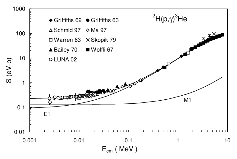
FIG. I.a.: ²H(p,$\gamma$)³He $S$ factor. The data are taken from Ref. [51] (Griffiths 62), Ref. [52] (Griffiths 63), Ref. [53] (Warren 63), Ref. [54] (Wolfli 67), Ref. [55] (Bailey 70), Ref. [56] (Skopic 79), Ref. [31] (Schmid 97), Ref. [57] (Ma 97), and Ref. [17] (LUNA 02).

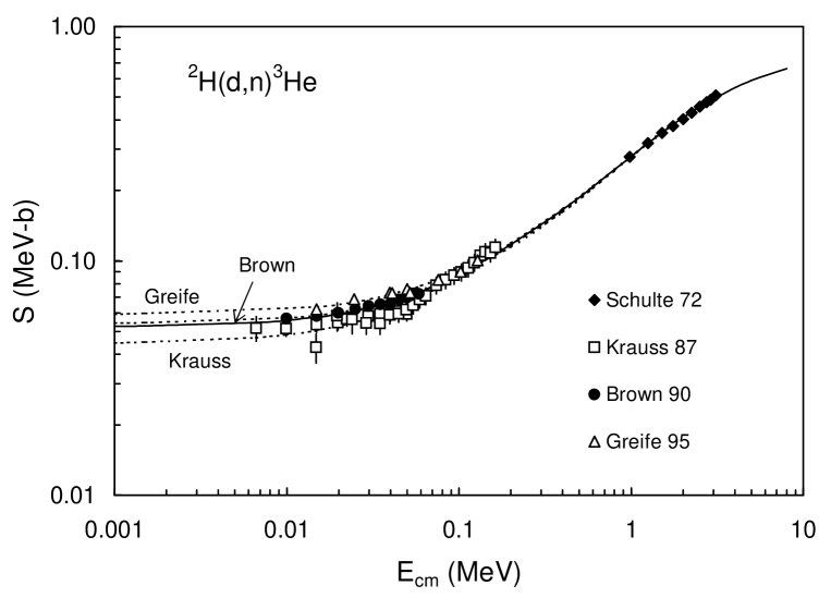
FIG. I.b.: ²H(d,n)³He $S$ factor. The data are taken from Ref. [35] (Schulte 72), Ref. [32] (Krauss 87), Ref. [33] (Brown 90), and Ref. [34] (Greife 95). The dotted curves represent the individual fits.

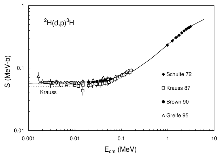
FIG. I.c.: ²H(d,p)³H $S$ factor. The data are taken from Ref. [35] (Schulte 72), Ref. [32] (Krauss 87), Ref. [33] (Brown 90), and Ref. [34] (Greife 95). The dotted curve represents the individual fit to Ref. [32]. Individual fits of Ref. [33] and [34] are very close to the global fit.

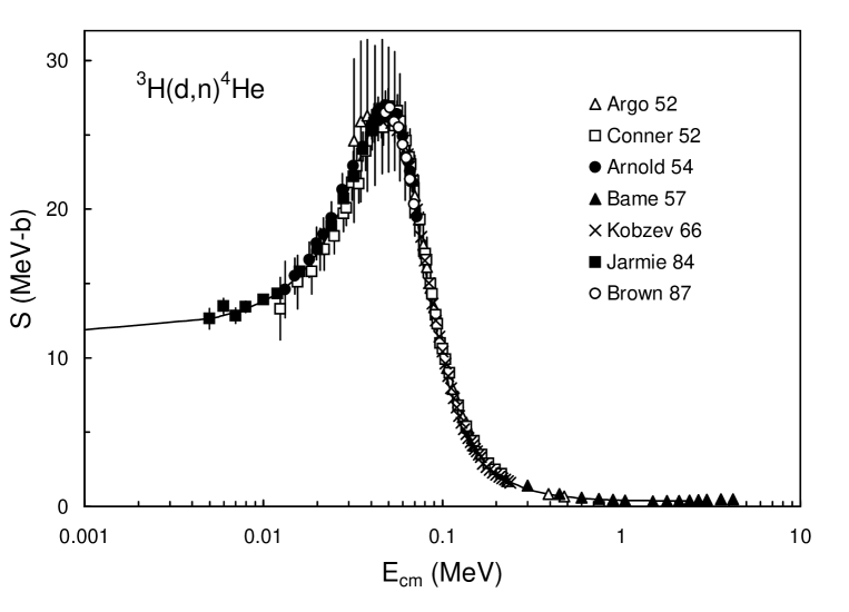
FIG. I.d.: ³H(d,n)⁴He $S$ factor. The data are taken from Ref. [58] (Argo 52), Ref. [59] (Conner 52), Ref. [60] (Arnold 54), Ref. [61] (Bame 57), Ref. [62] (Kobzev 66), Ref. [63] (McDaniels), Ref. [64] (Jarmie 84), and Ref. [65] (Brown 87).

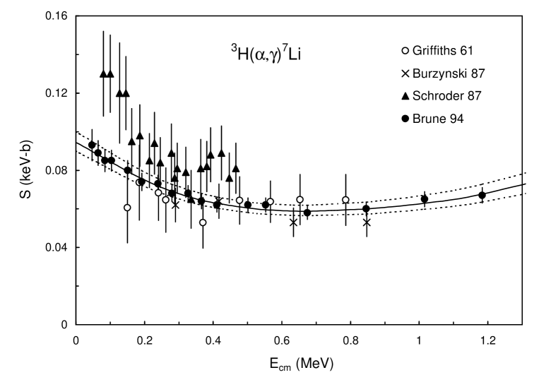
FIG. I.e.: ³H($\alpha,\gamma)^{7}$Li $S$ factor. The data are taken from Ref. [37] (Griffiths 61), Ref. [66] (Burzyński 87), Ref. [38] (Schröder 87), and Ref. [67] (Brune 94).

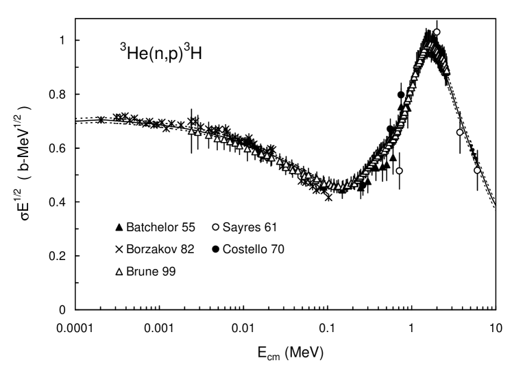
FIG. I.f.: ³He(n,p)³H cross section $(\times\sqrt{E})$. The data are taken from Ref. [68] (Batchelor 55), Ref. [69] (Sayres 61), Ref. [70] (Costello 70), Ref. [71] (Borzakov 82), and Ref. [16] (Brune 99).

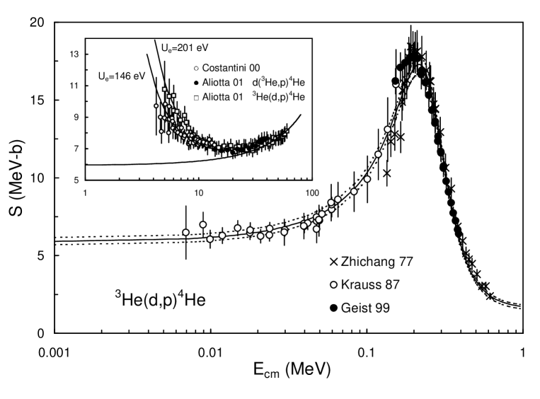
FIG. I.g.: ³He(d,p)⁴He $S$ factor. The data are taken from Ref. [40] (Krauss 87), Ref. [72] (Zhichang 75), Ref. [73] (Geist 99), Ref. [41] (Costantini 00) and Ref. [42] (Aliotta 01). The insert shows the influence of electron screening (energies are given in keV).

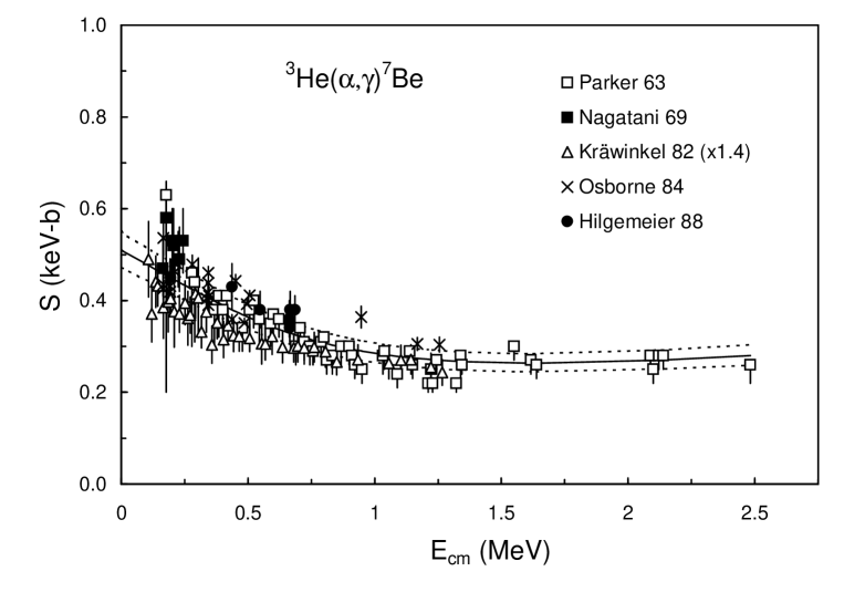
FIG. I.h.: ³He($\alpha,\gamma)^{7}$Be $S$ factor. The data are taken from Ref. [74] (Parker 63), Ref. [45] (Nagatani 69), Ref. [47] (Kräwinkel 82), Ref. [75] (Osborne 84), and Ref. [46] (Hilgemeier 88).

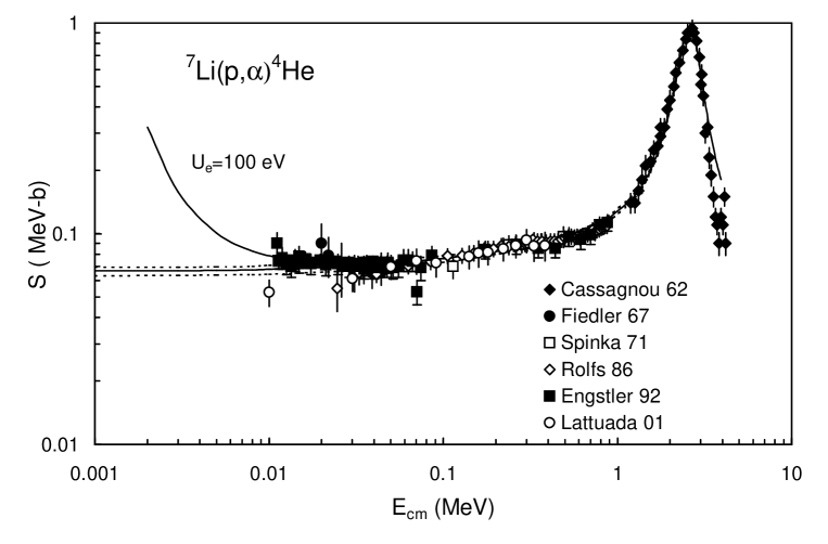
FIG. I.i.: ⁷Li(p,$\alpha)\alpha$ $S$ factor. The data are taken from Ref. [76] (Cassagnou 62), Ref. [77] (Fiedler 67), Ref. [78] (Spinka 71), Ref. [79] (Rolfs 86), Ref. [80] (Engstler 92), and Ref. [49] (Lattuada 01).

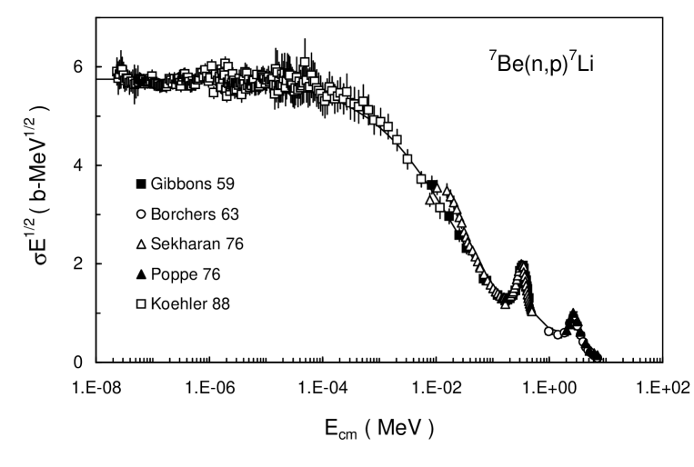
FIG. I.j.: ⁷Be(n,p)⁷Li cross section $(\times\sqrt{E})$. The data are taken from Ref. [81] (Gibbons 59), Ref. [82] (Borchers 63), Ref. [83] (Sekharan 76), Ref. [84] (Poppe 76), and Ref. [85] (Koehler 88).

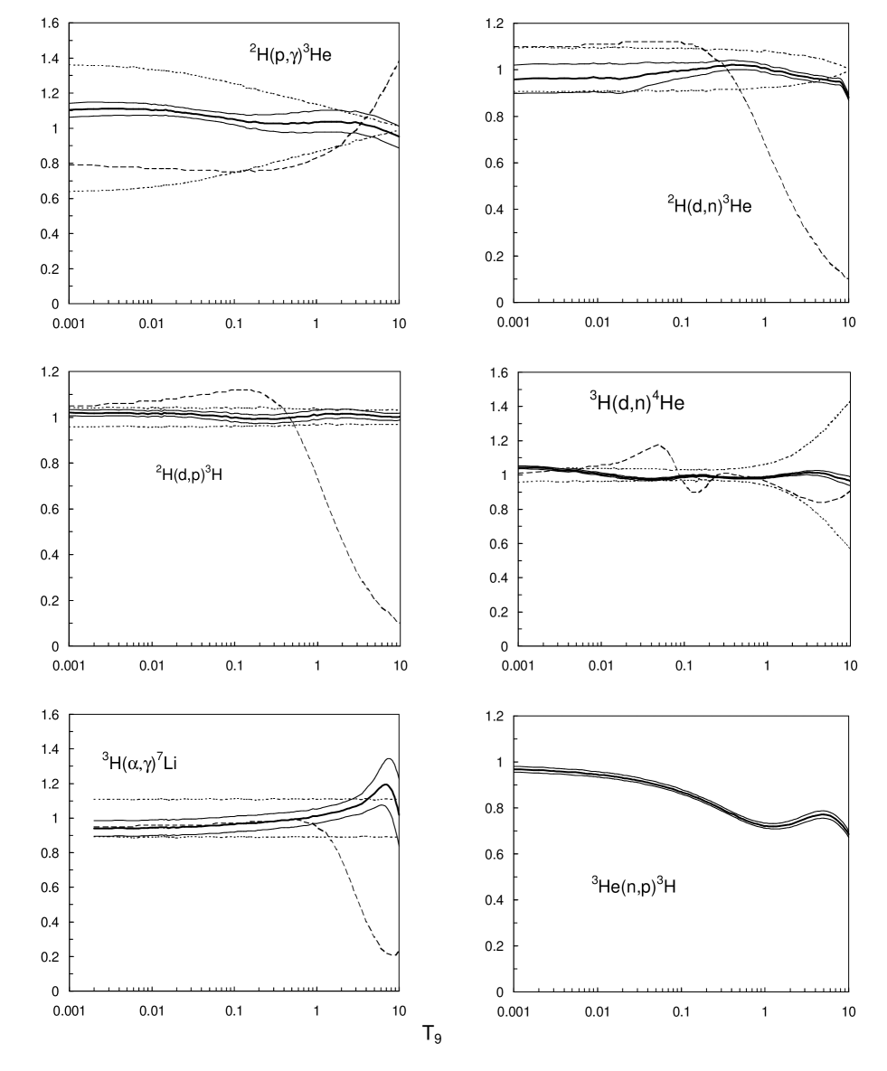
FIG. II.a.: Ratios of the present reaction rates to the NACRE and SKM rates.

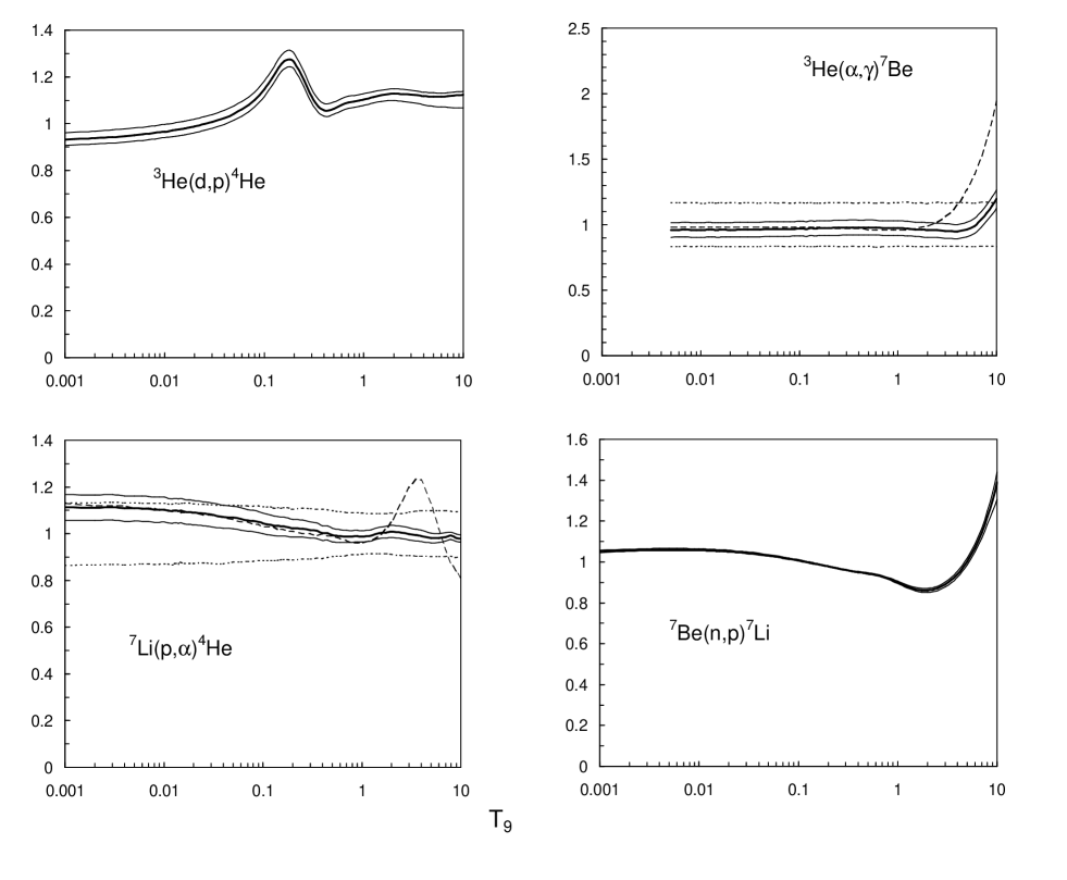
FIG. II.b.: Ratios of the present reaction rates to the NACRE and SKM rates.

REFERENCES

- [1] K.A. Olive, G. Steigman and T.P. Walker, Phys. Rep. 333–334 389 (2000)
- [2] A. Coc, E. Vangioni-Flam, M. Cassé and M. Rabiet, Phys. Rev. D65 043510 (2002)
- [3] K.A. Olive, Proc. International Symposium on Cosmology and Particle Astrophysics, 2002, National Taiwan University Taipei, Taiwan, to be published.
- [4] D.N. Spergel, L. Verde, H.V. Peiris, E. Komatsu, M.R. Nolta, C.L. Bennett, M. Halpern, G. Hinshaw, N. Jarosik, A. Kogut, M. Limon, S.S. Meyer, L. Page, G.S. Tucker, J.L. Weiland, E. Wollack, and E.L. Wright, submitted to Astrophys. J. (astro-ph/0302209)
- [5] G.R. Caughlan and W.A. Fowler, At. Data Nucl. Data Tables 40, 283 (1988)
- [6] C. Angulo, M. Arnould, M. Rayet, P. Descouvemont, D. Baye, C. Leclercq-Willain, A. Coc, S. Barhoumi, P. Auger, C. Rolfs, R. Kunz, J.W. Hammer, A. Mayer, T. Paradellis, S. Kossionides, C. Chronidou, K. Spyrou, S. Degl’Innocenti, G. Fiorentini, B. Ricci, S. Zavatarelli, C. Providencia, H. Wolters, J. Soares, C. Grama, J. Rahighi, A. Shotter and M. Lamehi-Rachti, Nucl. Phys. A656, 3 (1999)
- [7] E. Vangioni-Flam, A. Coc, and M. Cassé, Astron. Astrophys. 360 15 (2000)
- [8] R.H. Cyburt, B.D. Fields, and K.A. Olive , New Astronomy 6, 215 (2001).
- [9] M.S. Smith, L.H. Kawano, and R.A. Malaney, Astrophys. J. S. 85, 219 (1993)
- [10] K.M. Nollett and S. Burles, Phys. Rev. D61, 123505 (2000)
- [11] D.D. Clayton, in “Principles of stellar evolution and nucleosynthesis”, The University of Chicago Press (1983).
- [12] L.M. Krauss and P. Romanelli, Astrophys. J. 358, 47 (1990)
- [13] T.P. Walker, G. Steigman, D.N. Schramm, K.A. Olive, and H.-S. Kang, Astrophys. J. 376, 51 (1991)
- [14] A.M. Lane and R.G. Thomas, Rev. Mod. Phys. 30, 257 (1958)
- [15] Particle Data Group, K. Hagiwara et al., Phys. Rev. D66, 010001 (2002)
- [16] C.R. Brune, K.I. Hahn, R.W. Kavanagh and P.W. Wrean, Phys. Rev. C60, 015801 (1999)
- [17] LUNA Collaboration, C. Casella, H. Costantini, A. Lemut, B. Limata, R. Bonetti, C. Broggini, L. Campajola, P. Corvisiero, J. Cruz, A. D’Onofrio, A. Formicola, Z. Fülöp, G. Gervino, L. Gialanella, A. Guglielmetti, C. Gustavino, G. Gyurky, G. Imbriani, A.P. Jesus, M. Junker, A. Ordine, J.V. Pinto, P. Prati, J.P. Ribeiro, V. Roca, D. Rogalla, C. Rolfs, M. Romano, C. Rossi-Alvarez, F. Schuemann, E. Somorjai, O. Straniero, F. Strieder, F. Terrasi, H.P. Trautvetter and S. Zavatarelli, Nucl. Phys. A706, 203 (2002)
- [18] J.-W. Chen and M.J. Savage, Phys. Rev. C60, 015801 (1999)
- [19] E. Vangioni-Flam, A. Coc, P. Descouvemont, A. Adahchour, M. Cassé and C. Angulo, Astrophys. J. 600, 544 (2004).
- [20] R.G. Thomas, Phys. Rev. 88, 1109 (1952)
- [21] C. Angulo and P. Descouvemont, Phys. Rev. C61, 064611 (2000)
- [22] C. Brune, Phys. Rev. C66, 044611 (2002)
- [23] C. Angulo and P. Descouvemont, Nucl. Phys. A639, 733 (1998)
- [24] Numerical Recipes, by W.H. Press et al., Cambridge University Press (Cambridge), 1986
- [25] G. Audi and A.H. Wapstra, Nucl. Phys. A595, 409 (1995)
- [26] W.A. Fowler, G.R. Caughlan, and B.A. Zimmerman, Ann. Rev. Astron. Astrophys. 5, 525 (1967)
- [27] H.J. Assenbaum, K. Langanke and C. Rolfs, Z. Phys. A327, 461 (1987)
- [28] F.C. Barker, Nucl. Phys. A707, 277 (2002)
- [29] G. Audi, O. Bersillon, J. Blachot, and A.H. Wapstra, Nucl. Phys. A624, 1 (1997)
- [30] G.J. Schmid, R.M. Chasteler, C.M. Laymon, H.R. Weller, R.M. Prior, and D.R. Tilley, Phys. Rev. C52, R1732 (1995)
- [31] G.J. Schmid, B.J. Rice, R.M. Chasteler, M.A. Godwin, G.C. Kiang, L.L. Kiang, C.M. Laymo, R.M. Prior, D.R. Tilley, and H.R. Weller, Phys. Rev. C56, 2565 (1997)
- [32] A. Krauss, H.W. Becker, H.P. Trautvetter, C. Rolfs, and K. Brand, Nucl. Phys. A465, 150 (1987)
- [33] R.E. Brown and N. Jarmie, Phys. Rev. C41, 1391 (1990)
- [34] U. Greife, F. Gorris, M. Junker, C. Rolfs, and D. Zahnow, Z. Phys. A351, 107 (1995)
- [35] R.L. Schulte, M. Cosack, A.W. Obst, and J.L. Weil, Nucl. Phys. A192, 609 (1972)
- [36] G.M. Hale, document available at http://t2.lanl.gov/data/astro/astro.html.
- [37] G.M. Griffiths, R.A. Morrow, P.J. Riley, and J.B. Warren, Can. J. Phys. 39, 1397 (1961)
- [38] U. Schröder, A. Redder, C. Rolfs, R.E. Azuma, L. Buchmann, C. Campbell, J.D. King, and T.R. Donoghue, Phys. Lett. B192, 55 (1987)
- [39] A. Adahchour and P. Descouvemont, J. Phys. G29, 395 (2003)
- [40] A. Krauss, H.W. Becker, H.P. Trautvetter, C. Rolfs, and K. Brand, Nucl. Phys. A465, 150 (1987)
- [41] H. Costantini, A. Formicola, M. Junker, R. Bonetti, C. Broggini, L. Campajola, P. Corvisiero, A. D’Onofrio, A. Fubini, G. Gervino, L. Gialanella, U. Greife, A. Guglielmetti, C. Gustavino, G. Imbriani, A. Ordine, P.G. Prada Moroni, P. Prati, V. Roca, D. Rogalla, C. Rolfs, M. Romano, F. Schümann, O. Straniero, F. Strieder, F. Terrasi, H.-P. Trautvetter and S. Zavatarelli, Phys. Lett. 482B, 43 (2000)
- [42] M. Aliotta, F. Raiola, G. Gy rky, A. Formicola, R. Bonetti, C. Broggini, L. Campajola, P. Corvisiero, H. Costantini, A. D’Onofrio, Z. Fülöp, G. Gervino, L. Gialanella, A. Guglielmetti, C. Gustavino, G. Imbriani, M. Junker, P.G. Moroni, A. Ordine, P. Prati, V. Roca, D. Rogalla, C. Rolfs, M. Romano, F. Sch mann, E. Somorjai, O. Straniero, F. Strieder, F. Terrasi, H.-P. Trautvetter and S. Zavatarelli, Nucl. Phys. A690, 790 (2001)
- [43] S. Engstler, A. Krauss, K. Neldner, C. Rolfs, U. Schröder, and K.Langanke, Phys. Lett. 202B, 179 (1988)
- [44] P. Prati, C. Arpesella, F. Bartolucci, H. W. Becker, E. Bellotti, C. Broggini, P. Corvisiero, G. Fiorentini, A. Fubini, G. Gervino, F. Gorris, U. Greife, C. Gustavino, M. Junker, C. Rolfs, W. H. Schulte, H. P. Trautvetter, and D. Zahnow, Z. Phys. A350, 171 (1994)
- [45] K. Nagatani, M.R. Dwarakanath, and D. Ashery, Nucl. Phys. A128, 325 (1969)
- [46] M. Hilgemeier, H.W. Becker, C. Rolfs, H.P. Trautvetter, and J.W. Hammer, Z. Phys. A329, 243 (1988)
- [47] H. Kräwinkel, H.W. Becker, L. Buchmann, J. Görres, K.U. Kettner, W. E. Kieser, R. Santo, P. Schmalbrock, H.P. Trautvetter, A. Vlieks, C. Rolfs, J.W. Hammer, R.E. Azuma, and W.S. Rodney, Z. Phys. A304, 307 (1982)
- [48] E.G. Adelberger, S.M. Austin, J.N. Bahcall, A.B. Balantekin, G. Bogaert, L.S. Brown, L. Buchmann, F.E. Cecil, A.E. Champagne, L. de Braeckeleer, C.A. Duba, S.R. Elliot, S.J. Freedman, M. Gai, G. Goldring, C.R. Gould, A. Gruzinov, W.C. Haxton, K.M. Heeger, E. Henley, C.W. Johnson, M. Kamionkowski, R.W. Kavanagh, S.E. Koonin, K. Kubodera, K. Langanke, T. Motobayashi, V. Pandharipande, P. Parker, R.G.H. Robertson, C. Rolfs, R.F. Sawyer, N. Shaviv, T.D. Shoppa, K.A. Snover, E. Swanson, R.E. Tribble, S. Turck-Chièze, and J.F. Wilkerson, Rev. Mod. Phys. 70, 1265 (1998)
- [49] M. Lattuada, R.G. Pizzone, S. Typel, P. Figuera, A. Musumarra, M.G. Pellegriti, A. Miljanic, C. Rolfs, C. Spitaleri, and H.H. Wolter, Ap. J. 562, 1076 (2001)
- [50] F.C. Barker, Phys. Rev. C62, 044607 (2000)
- [51] G.M. Griffiths, E.A. Larson, and L.P. Robertson, Can. J. Phys. 40, 402 (1962)
- [52] G.M. Griffiths, M. Lal, and C.D. Scarfe, Can. J. Phys. 41, 724 (1963).
- [53] J.B. Warren, K.L. Erdman, L.P. Robertson, D.A. Axen, and J.R. Macdonald, Phys. Rev. 132, 1691 (1963)
- [54] W. Wolfli, R. Bösch, J. Lang, R. Müller, and P. Marmier, Helv. Phys. Acta 40, 946 (1967)
- [55] G.M. Bailey , G.M. Griffiths, M.A. Olivio, and R.L. Helmer, Can J. Phys. 48, 3059 (1970)
- [56] D.M. Skopik, H.R. Weller, N.R. Roberson, and S.A. Wender, Phys. Rev. C19, 601 (1979)
- [57] L. Ma, H.J. Karwowski, C.R. Brune, Z. Ayer, T.C. Black, J.C. Blackmon, E.J. Ludwig, M. Viviani, A. Kievsky, and R. Schiavilla, Phys. Rev. C55, 588 (1997)
- [58] H.V. Argo, R.F. Taschek, H.M. Agnew, A. Hemmendinger, and W.T. Leland, Phys. Rev. 87, 612 (1952)
- [59] J.P. Conner, T.W. Bonner, and J.R. Smith, Phys. Rev. 88, 468 (1952)
- [60] W.R. Arnold, J.A. Phillips, G.A. Sawyer, E.J. Stovall Jr, and J.L. Tuck, Phys. Rev. 93, 483 (1954)
- [61] S.J. Bame Jr, and J.E. Perry Jr, Phys. Rev. 107, 1616 (1957)
- [62] A.P. Kobzev, V.I. Salatskii, and S.A. Telezhnikov, Sov. J. Nucl. Phys. 3, 774 (1966)
- [63] D.K. McDaniels, M. Drosg, J.C. Hopkins, and J.D. Seagrave, Phys. Rev. C7, 882 (1973)
- [64] N. Jarmie, R.E. Brown, and R.A. Hardekopf, Phys. Rev. C29, 2031 (1984)
- [65] R.E. Brown, N. Jarmie, and G.M. Hale, Phys. Rev. C35, 1999 (1987)
- [66] S. Burzyński, K. Czerski, A. Marcinkowski, and P. Zupranski, Nucl. Phys. A473, 179 (1987)
- [67] C.R. Brune, R.W. Kavanagh, and C. Rolfs, Phys. Rev. C50, 2205 (1994)
- [68] R. Batchelor, R. Aves, and T.H.R. Shyrme, Rev. Sci. Instrum. 26, 1037 (1955)
- [69] A.R. Sayres, K.W. Jones, and C.S. Wu, Phys. Rev. 122, 1853 (1961)
- [70] D.G. Costello, S. J. Friesenhahn, and W. M. Lopez, Nucl. Sci. Eng. 39, 409 (1970)
- [71] S.B. Borzakov, H. Malecki, L.B. Pikel’ner, M. Stempinski, and E.I. Sharapov, Yad. Fiz. 35, 532 (1982) [Sov. J. Nucl. Phys.] 35, 307 (1982)
- [72] L. Zhichang, Y. Jingang, D. Xunliang, Chin. J. Sci. Tech. At. Energy 3, 229 (1977), in chinese, from CSISRS database.
- [73] W.H. Geist, C.R. Brune, H.J. Karwowski, E.J. Ludwig, K.D. Veal, and G.M. Hale, Phys. Rev. C60, 054003 (1999)
- [74] P.D. Parker and R.W. Kavanagh, Phys. Rev. 131, 2578 (1963)
- [75] J.L. Osborne, C.A. Barnes, R.W. Kavanagh, R.M. Kremer, G.J. Mathews, J.L. Zyskind, P.D. Parker, and A.J. Howard, Nucl. Phys. A419, 115 (1984)
- [76] Y. Cassagnou, J.M.F. Jeronymo, G.S. Mani, A. Sadeghi, and P.D. Forsyth, Nucl. Phys. 33, 449 (1962); 41, 176 (1963)
- [77] O. Fiedler and P. Kunze, Nucl. Phys. A96, 513 (1967)
- [78] H. Spinka, T. Tombrello, and H. Winkler, Nucl. Phys. A164, 1 (1971)
- [79] C. Rolfs and R.W. Kavanagh, Nucl. Phys. A455, 179 (1986)
- [80] S. Engstler, G. Raimann, C. Angulo, U. Greife, C. Rolfs, U. Schröder, E. Somorjai, B. Kirch, and K. Langanke, Z. Phys. A342, 471 (1992); Phys. Lett. B279, 20 (1992)
- [81] J.H. Gibbons and R.L. Macklin, Phys. Rev. 114, 571 (1959)
- [82] R.R. Borchers and C.H. Poppe, Phys. Rev. 129, 2679 (1963)
- [83] K.K. Sekharan, H. Laumer, B. D. Kern and Gabbard, Nucl. Instr. Meth. 133, 253 (1976)
- [84] C.H. Poppe, J.D. Anderson, J.C. Davis, S. M. Grimes and C. Wong, Phys. Rev. C14, 438 (1976)
- [85] P.E. Koehler, C.D. Bowman, F.J. Steinkruger, D.C. Moody, G.H. Hale, J.W. Starner, S.A. Wender, R.C. Haight, P.W. Lisowski and W.L. Talbert, Phys. Rev. C37, 917 (1988)